| Issue |
A&A
Volume 688, August 2024
|
|
|---|---|---|
| Article Number | A155 | |
| Number of page(s) | 10 | |
| Section | Astrophysical processes | |
| DOI | https://doi.org/10.1051/0004-6361/202449846 | |
| Published online | 14 August 2024 | |
Characterization of carbon dioxide on Ganymede and Europa supported by experiments: Effects of temperature, porosity, and mixing with water
1
Faculty of Aerospace Engineering, Delft University of Technology, Delft, The Netherlands
2
Centro de Astrobiología (CSIC-INTA), Ctra. de Ajalvir, km 4, Torrejón de Ardoz, 28850 Madrid, Spain
3
Leiden Observatory, Leiden University, PO Box 9513 2300 RA Leiden, The Netherlands
4
Department of Physics, National Central University, Jhongli City, Taoyuan County 32054, Taiwan
5
Max Planck Institute for Extraterrestrial Physics, Postfach 1312, 85741 Garching, Germany
Received:
4
March
2024
Accepted:
18
April
2024
Abstract
Context. The surfaces of icy moons are primarily composed of water ice that can be mixed with other compounds, such as carbon dioxide. The carbon dioxide (CO2) stretching fundamental band observed on Europa and Ganymede appears to be a combination of several bands that are shifting location from one moon to another.
Aims. We investigate the cause of the observed shift in the CO2 stretching absorption band experimentally. We also explore the spectral behaviour of CO2 ice by varying the temperature and concentration.
Methods. We analyzed pure CO2 ice and ice mixtures deposited at 10 K under ultra-high vacuum conditions using Fourier-transform infrared (FTIR) spectroscopy and temperature programmed desorption (TPD) experiments. Laboratory ice spectra were compared to JWST observation of Europa’s and Ganymede’s leading hemispheres. The simulated IR spectra were calculated using density functional theory (DFT) methods, exploring the effect of porosity in CO2 ice.
Results. Pure CO2 and CO2-water ice show distinct spectral changes and desorption behaviours at different temperatures, revealing intricate CO2 and H2O interactions. The number of discernible peaks increases from two in pure CO2 to three in CO2-water mixtures.
Conclusions. The different CO2 bands were assigned to ν̃3,1 (2351 cm−1, 4.25 μm) caused by CO2 dangling bonds (CO2 found in pores or cracks) and ν̃3,2 (2345 cm−1, 4.26 μm) due to CO2 segregated in water ice, whereas ν̃3,3 (2341 cm−1, 4.27 μm) is due to CO2 molecules embedded in water ice. The JWST NIRSpec CO2 spectra for Ganymede and for Europa can be fitted with two Gaussians attributed to ν̃3,1 and ν̃3,3. For Europa, ν̃3,1 is located at lower wavelengths due to a lower temperature. The Ganymede data reveal latitudinal variations in CO2 bands, with ν̃3,3 dominating in the pole and ν̃3,1 prevalent in other regions. This shows that CO2 is embedded in water ice at the poles and it is present in pores or cracks in other regions. Ganymede longitudinal spectra reveal an increase of the CO2 ν̃3,1 band throughout the day, possibly due to ice cracks or pores caused by large temperature fluctuations.
Key words: methods: laboratory: solid state / methods: numerical / methods: observational / planets and satellites: composition / infrared: planetary systems
Corresponding author; This email address is being protected from spambots. You need JavaScript enabled to view it. .
© The Authors 2024
 Open Access article, published by EDP Sciences, under the terms of the Creative Commons Attribution License (https://creativecommons.org/licenses/by/4.0), which permits unrestricted use, distribution, and reproduction in any medium, provided the original work is properly cited.
This article is published in open access under the Subscribe to Open model. This email address is being protected from spambots. You need JavaScript enabled to view it. to support open access publication.
1. Introduction
Mixed ices of CO2 and water are known to be present in the frozen nuclei of comets (Crovisier 2006a,b) in various satellites of our Solar System (e.g. Grundy et al. 2003; Buratti et al. 2005) and as components of dust interstellar particles (e.g. Dartois et al. 2005; Draine 2003). On Ganymede, the CO2 stretching fundamental band, which is ordinarily at 2341 cm−1 (4.27 μm) (Falk 1987), has been observed with the Near Infrared Mapping Spectrometer (NIMS) aboard the Galileo spacecraft (McCord et al. 1998). The location of this absorption band is displaced slightly to a shorter wavelength (2345 cm−1, 4.26 μm) indicating that the CO2 is bound, or trapped, in a host. Recent James Webb Space Telescope (JWST) observations (Bockelée-Morvan et al. 2024) have shown variations in the latitude and longitude of the CO2 bands on Ganymede’s surface. In the boreal region of the leading hemisphere, the CO2 band is dominated by the 2341 cm−1 (4.27 μm) band, consistent with CO2 trapped in amorphous water ice, while at equatorial latitudes (and especially on dark terrains) the observed band is broader and located around 2345 cm−1 (4.26 μm), suggesting CO2 adsorbed on non-icy materials, such as minerals or salts. On Europa, CO2 was detected with the Galileo/NIMS instrument at 2351 cm−1 (4.25 μm) and mostly located on the anti-Jovian and trailing sides (Hansen & McCord 2008); however, observations in the near-infrared (NIR) were not able to confirm the presence of CO2 (Mishra et al. 2021). Recent JWST observations by Villanueva et al. (2023) have highlighted the presence of CO2 on Europa’s surface, with bands located at 2351 cm−1 (4.25 μm) and 2341 cm−1 (4.27 μm). These observations suggest that CO2 is mixed with other compounds and that carbon is sourced from within Europa, probably from the liquid sub-surface ocean.
Prompted by these findings, solid H2O/CO2 ice mixtures, as laboratory analogues of astrophysical objects, have been studied for many years, mainly by infrared spectroscopy and mass spectrometry, in controlled warm-up experiments (i.e. Sandford & Allamandola 1990; Ehrenfreund et al. 1997; Bernstein et al. 2005; Kumi et al. 2006; Malyk et al. 2007). From these studies, the interaction between CO2 and H2O on a molecular level has been shown to cause significant changes in the position and profile of CO2 peaks in the IR. However, a concise answer to why the CO2 stretching fundamental band on icy moons, like Europa and Ganymede, shows frequency shifts remains elusive.
In the present work, we attempt to find an explanation for the different CO2 bands to characterise the carbon dioxide on Europa and Ganymede. This is achieved by investigating the influence of temperature on the spectral properties of laboratory CO2 ice, and in particular the behaviour of the CO2 stretching mode, which (in its pure form) peaks around 2344 cm−1 (4.27 μm). We note that CO2 is first studied in its pure form and afterwards co-deposited with water so that the H2O:CO2 deposition ratio is varied. In particular, we considered low (< 5%) and high (> 25%) carbon dioxide concentrations in the ice. Experiments were carried out at temperatures ranging between 10 K and 160 K and ultra high vacuum conditions. This research uses a combination of the following two techniques: temperature programmed desorption (TPD) and Fourier-transform infrared spectroscopy (FTIR) in transmittance, across a variety of experimental conditions. Additionally, Gaussian deconvolution was applied to the spectra obtained experimentally. This technique was first applied to pure CO2 ice and afterwards to the ice mixture H2O:CO2. It was found that deconvolution of the asymmetric stretching band ν3 requires two Gaussians for pure CO2 and three when mixed with water. The evolution of the integrated absorbance areas, band shape and position as a function of temperature can be compared to the TPD curve in order to assign the bands to different molecular interactions, thus characterising the type of CO2 ice. The synergy between laboratory studies and data gathered by JWST enriches our comprehensive approach to understanding CO2 behaviour on icy worlds, enabling a thorough exploration of the fundamental properties of CO2 ice in various conditions.
The structure of this paper is organized as follows. In Sect. 2, we outline the experimental setup and the determination of the gas mixture ratio. In Sect. 3, we focus on the spectroscopic behaviour of pure CO2 ice, elucidating the shape and location of the ν3 stretching band, alongside the TPD curve. In Sects. 4 and 5, we describe the acquired laboratory spectra for low and high CO2 concentrations in water ice as a function of temperature, accompanied by explanations of integrated absorbance areas and TPD curves. In Sects. 6 and 7, we discuss the results and assign the IR vibrational modes from experiments and simulations. Finally, Sect. 8 delves into the application of findings to icy moons, specifically Europa and Ganymede, involving a comparison of new experimental results with recent observations.
2. Experimental method
2.1. ISAC set-up
The experiments reported in this work have been performed with the Interstellar Astrochemistry Chamber (ISAC), described in more detail in Muñoz Caro et al. (2010). ISAC is an ultra-high vacuum (UHV) chamber with a base pressure of 4 × 10⁻¹¹ mbar, designed to simulate the conditions present in the interstellar medium (ISM), regarding temperature, pressure and ultraviolet (UV) radiation field. A closed-cycle He cryostat allows for the tip of the cold finger to cool down to 8 K, where a sample holder with a potassium bromide (KBr) window acting as the substrate for ice deposition is located. A schematic representation is shown in Fig. 1. A Lakeshore temperature controller 331 with 0.1 K accuracy was used. The gas line, which permits the introduction of gas species with regulated compositions, is linked to the main chamber through a leak valve. The identification of the species present in the chamber is done via a quadrupole mass spectrometer (QMS, Pfeiffer Vacuum, Prisma QMS 200). The valve is opened during deposition, and the gas is delivered to the cold substrate through a deposition tube. This tube’s end is roughly placed at a distance of 3 cm from the substrate. FTIR in transmittance mode using a Bruker Vertex 70 at a working spectral resolution of 2 cm−1 is used to record infrared spectra during deposition, and later during the TPD using a heating ramp in K/min. ISAC uses laser interferometry at 632.8 nm to assess changes in ice thickness (González Díaz et al. 2022). A 5.0 mW He-Ne red laser and a Silicon Photodiode Power Sensor to measure the optical power of the laser light (model S120C) are mounted at an angle of 6°, as seen in Fig. 1.
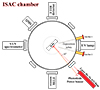 |
Fig. 1. ISAC cross-section at the ice sample level. The measuring devices and sensors, including the laser interferometry, are displayed. The FTIR source is positioned on one side and the FTIR detector on the opposite one. The UV spectrometer is placed directly across from the vacuum-UV lamp, see González Díaz et al. (2022) for more details. |
In general, ices were grown at 10 K by opening the leak valve of gas line 2 in Fig. 1, feeding a mixture of H2O and CO2 into the main chamber, at a deposition pressure of 2 × 10⁻⁷ mbar. To investigate the influence of deposition temperature and pressure on the spectral properties of CO2 ice (in particular, the behaviour of the CO2 stretching mode), some experiments were also carried out at 70 K and higher deposition pressure. The experiments presented in Table 1 were repeated for reproducibility or for suspected contamination. During the deposition of the gas mixture to form the ice, infrared spectra at 45° incidence of the beam relative to the substrate were collected every 300 s. Warming up the samples after deposition was done at 0.2 K min−1 until a temperature of 210 K was attained, ensuring that both the CO2 and H2O were entirely desorbed. IR measurements were taken every 300 s again, yielding a spectrum every 1 K temperature increment.
Experimental parameters.
The key parameters measured during the experiments using various devices include: the laser intensity to measure the ice thickness (González Díaz et al. 2022), pressure inside the chamber, the ion currents of the relevant molecules (via QMS), and temperature. The temperature of the ice sample was measured using a silicon diode sensor connected to the sample holder and placed directly above the ice sample. A Bayard-Alpert gauge positioned about 23 cm below the plane where deposition occurs was used to measure the pressure in the main chamber of ISAC. Laser interference was monitored continuously, resulting in an interference pattern during ice deposition and a new interference pattern during TPD. The ice column density was calculated using IR spectroscopy from the areas calculated by integration of the absorption bands. This is covered in more detail in the following section.
2.2. Estimation of the ice mixture ratio
The integration of the infrared absorption band yields the column density N of the ice layer accreted on the cold substrate in molecules cm−2 with the following formula:
 (1)
(1)
with A the band strength in cm molecule−1, τν the optical depth of the band and dν the wavenumber differential in cm−1. The integrated absorbance is equal to 0.43 × τ, where τ is the integrated optical depth of the band. The ice mixture ratio is calculated by dividing the column density of the carbon dioxide anti-symmetric stretching band to the water stretching band. The IR band strength of the CO2 str. feature in the H2O:CO2 = 24:1 ice mixture is about 94% with respect to the pure CO2 ice (from Table 3 of Gerakines et al. 1995), and for higher CO2 concentrations this difference is expected to be smaller. We therefore used the band strengths of pure ices at 10 K: A(H2O) = 2.0 × 10⁻¹⁶ cm molecule−1 (Hagen & Tielens 1981) and A(CO2) = 7.6 × 10⁻¹⁷ cm molecule−1 (Bouilloud et al. 2015). To compute the integrated intensities of the H2O stretching peaks, the measured peak positions and the integration limits in cm−1(μm) are taken between 3000 (3.33) and 3600 (2.78). The same method is applied to the CO2 anti-symmetric stretching mode in the 2330 (4.29) to 2360 (4.24) spectral range. A table summarizing the experimental parameters can be found in Table 1, where pdep is the total pressure in the ISAC chamber during deposition of the ice, Tdep is the temperature at which the ice is deposited, dice is the ice thickness, and dT/dt is the heating rate in Kelvin per minute.
3. Pure CO2 ice
Pure CO2 ice was deposited at 10 K and warmed up until 100 K. The study of the CO2 ice stretching band, commonly known as ν3, as well as the TPD are reported in Sections 3.1 and 3.2, respectively.
3.1. ν3 stretching band shape and position
Figure 2 shows the CO2 (ν3) asymmetric stretching fundamental for 12CO2 when deposited at 10 K, at a pressure of 2 × 10⁻⁷ mbar and warmed-up with a rate of 0.5 K/min up to 90 K. All the FTIR spectra have a resolution of 2 cm−1 and are shifted vertically for clarity. The 12CO2 asymmetric stretching fundamental (ν3) is located at ∼2345 cm−1 (4.26 μm), and is redshifted from the gas-phase value located at 2348 cm−1 (4.26 μm) due to interactions with the surrounding matrix environment (e.g. Isokoski et al. 2013). The profile is asymmetric with a prominent blue shoulder around 2350 cm−1 (4.25 μm). When the CO2 ice is warmed up, the main peak at 2345 cm−1 (4.26 μm) shifts to lower wavenumbers. In addition, the peak intensity increases with increasing temperature as a result of the decrease in bandwidth. Figure 3 illustrates the effect of temperature on the band’s shape and position.
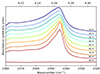 |
Fig. 2. Spectra over the 2380−2320 cm−1 (4.20−4.31 μm) range of a pure CO2 ice deposited at 10 K and 2 × 10⁻⁷ mbar, later warmed up to 90 K. All spectra are measured at 2 cm−1 resolution, and at temperatures indicated in each graph. Spectra are shifted vertically for clarity. |
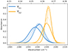 |
Fig. 3. Evolution of both Gaussian distributions during warm-up from 10 K to 80 K for a pure CO2 ice. The arrows indicate the direction of evolution. Thicker lines indicate the initial and final states. |
In general, each spectrum can be deconvolved into two Gaussian distributions, which we refer to as  at 2351 cm−1 (4.25 μm) and
  at 2345 cm−1 (4.26 μm), both for 10 K (see Table 2). The figure clearly shows the redshift of both Gaussians during warm-up as well as the decrease in FWHM for
  (2345 cm−1, 4.26 μm), going from 5.7 cm−1 at 10 K to 3.8 cm−1 at 80 K.
Band positions ( ) for all three fitted Gaussians as a function of temperature.
3.2. Thermal desorption of CO2
A TPD curve of a pure CO2 ice layer is shown in Fig. 4. The QMS data corresponding to the molecular mass of CO2 is plotted as the ion current in Ampere versus increasing temperature. This figure shows one desorption peak at 85 K. It is at this temperature that CO2 thermally desorbs. The desorption rate, expressed in molecules cm−2 s−1, of CO2 ice is described by the Polanyi-Wigner equation:
![Mathematical equation: $$ \begin{aligned} \frac{\mathrm{d}N_{\rm g}(\mathrm{CO}_2)}{\mathrm{d}t}=\nu _i[N_{\rm s}(\mathrm{CO}_2)]^i{\exp }\left(-\frac{E_{\rm d}(\mathrm{CO}_2)}{T}\right), \end{aligned} $$](/articles/aa/full_html/2024/08/aa49846-24/aa49846-24-eq25.gif) (2)
(2)
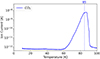 |
Fig. 4. TPD curve of pure CO2 ice layer deposited at 10 K and heated at 0.5 K/min. The ion current (A) is plotted on a logarithmic scale for a better appreciation of the curve profile and roughly corresponds to partial pressure in mbar. |
where Ng(CO2) is the column density of CO2 molecules that desorb from the ice surface (cm−2), νi is the frequency factor (molecules1 − i cm−2(1 − i) s−1) for desorption order, i, Ns(CO2) is the column density of CO2 molecules on the surface at time t, Ed(CO2) is the binding energy expressed in K, and T the surface temperature in K. The TPD data can be fitted using Eq. (2) and the relation:
 (3)
(3)
where  is the heating rate, 0.5 K min−1 in the reported experiments. Figure 5 shows the QMS data, column densities during warm-up, Polanyi-Wigner equation, and calculated zero-order coverage. The coverage is calculated using 1–
 . The TPD data were fitted using the parameter values ν0 = 0.4 × 1031 molecules cm−2 s−1 and Ed = 2555.78 K for the desorption of CO2 ice. We find that the coverage values determined by transmittance FTIR (green triangles) and the coverage curve computed by fitting the TPD curve recorded by QMS (light blue line) are in good agreement. There are only two remaining triangle datapoints that are poorly fitted. The issue is that a zero-order fit by definition fails when there are fewer than 4 × 10¹⁶ molecules per square centimeter of coverage, as demonstrated by Fig. 5.
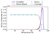 |
Fig. 5. Column density of CO2 ice (triangles) calculated from IR measurements matches the calculated coverage (light blue line). TPD curve of CO2 from QMS measurements (dark blue) agrees well with the fit corresponding to the Polanyi-Wigner equation (red line). |
4. Low CO2 concentration in water ice
A low CO2 content in the ice mixtures, up to 5%, is considered in this section. The important parameters of the presented experiments can be found in Table 1. Figure 6 depicts the spectra for a H2O:CO2 = 1:0.04 ratio deposited at 10 K. The experiment is performed with a deposition pressure of 2 × 10⁻⁷ mbar as reported in Table 1. At 10 K, the 12CO2 asymmetric stretching fundamental (ν3) can be deconvolved into three Gaussians in these experiments,  around 2351 cm−1 (4.25 μm),
  at 2345 cm−1 (4.26 μm), and
  at 2341 cm−1 (4.27 μm). The integrated absorbance area as a function of temperature is shown in the bottom panel of Fig. 7. Blue dots represent
  (2351 cm−1, 4.25 μm) starting at 10 K, which undergoes a red shift at elevated temperatures. Yellow triangles represent
  (2345 cm−1, 4.26 μm), which is red shifted by 1 cm−1 at 80 K right before thermal desorption. Green crosses representing
  (2341 cm−1, 4.27 μm) indicate no observable changes with increasing temperature.
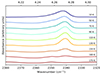 |
Fig. 6. Spectra over the 2380−2320 cm−1 (4.20−4.31 μm) range of the H2O:CO2 = 1:0.04 ice mixture deposited at 10 K and 2 × 10⁻⁷ mbar. All spectra are measured with 2 cm−1 resolution at the temperatures indicated in each graph. Spectra are shifted vertically for clarity. |
As mentioned before, pure CO2 ice thermally desorbs around 85 K. For the ice mixture H2O:CO2 = 1:0.04, the top panel of Fig. 7 shows the TPD curves from 10 K to 180 K, with three desorption peaks for carbon dioxide: one around 80 K, another one around 146 K, and a final one at 162 K, while only one peak appears for water, also at 162 K. There is a smaller CO2 desorption peak at 150 K which is not reproducible in repeated experiments and could be caused by a minor rearrangement of the water structure. The following explanation is given for the three main desorption peaks of carbon dioxide. Firstly, pure carbon dioxide ice thermally desorbs around 80 K, meaning that only CO2 molecules bonded with other CO2 molecules are desorbing. In second place, the peak at 140 K is caused by the transformation from cubic to hexagonal water ice (Martín-Doménech et al. 2014). During this process, carbon dioxide is pushed out of the water matrix. This peak is known as volcano desorption. The third peak between 160 and 170 K is the co-desorption of all remaining carbon dioxide along with water.
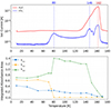 |
Fig. 7. TPD curves of CO2 and H2O for a H2O:CO2 = 1:0.04 ice heated at 0.2 K/min (top). Integrated absorbance areas of the three Gaussian distributions as a function of temperature for the same experiment (bottom). |
It is worth noting that carbon dioxide constantly desorbs between 80 and 146 K, as evidenced by the QMS signal being greater after the initial peak than before (see blue line in top panel of Fig. 7). This continuous desorption is caused by amorphous water ice rearrangement, which produces a change in the size and form of the porous structure (pores coalesce) when heated (Cazaux et al. 2015). Carbon dioxide molecules may diffuse through the pores and sublimate continuously between 80 and 146 K due to the increasing ice temperature and favored by this rearrangement. The argument of diffusing carbon dioxide molecules can be verified by looking at the integrated absorbance areas of the three Gaussian peaks in the bottom panel of Fig. 7. The data points (triangles) represent  (2345 cm−1, 4.26 μm) and confirm that pure CO2 desorbs thermally at 80 K. During this desorption of CO2 molecules starting at 75 K, the integrated area of
  (2341 cm−1, 4.27 μm) is increasing significantly, pointing towards the diffusion of the carbon dioxide molecules through the water ice structure. Once temperatures of 140 K are reached, the integrated areas of both
  (2351 cm−1, 4.25 μm) and
  (2341 cm−1, 4.27 μm) bands are continuously decreasing during annealing, confirming the amorphous water ice rearrangements. The cubic to hexagonal water-ice phase transition that occurs at 146 K further accelerates the desorption of CO2 molecules. Finally, any remaining CO2 will co-desorb with water around 162 K.
5. High CO2 concentration in water ice
In this section, a high CO2 content in the ice mixtures, above 20%, is considered. The parameters of the conducted experiments can be found in Table 1. Figure 8 shows the spectra for H2O:CO2 = 1:0.25 ice deposited at 10 K and 2 × 10⁻⁷ mbar. The broadening of the band is a consequence of the increased CO2 concentration, which causes particle aggregation and thus creates additional trapping sites between CO2 and H2O (Ehrenfreund et al. 1997). As with the low CO2 concentration, the spectra can be deconvolved into three Gaussian distributions, the band positions at 10 K are  = 2354 cm−1 (4.25 μm),
  = 2344 cm−1 (4.27 μm), and
  = 2336 cm−1 (4.28 μm), at 10 K. Due to the broadening of the CO2 band, the shoulder on the left is blueshifted by 2 cm−1, compared to the low CO2 concentration spectra at 10 K. In addition, the shoulder on the right is redshifted by 4 cm−1.
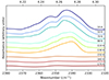 |
Fig. 8. Spectra over the 2380−2320 cm−1 (4.20−4.31 μm) range of the H2O:CO2 = 1:0.25 ice mixture deposited at 10 K and 2 × 10⁻⁷ mbar. All spectra are measured with 2 cm−1 resolution at the temperatures indicated in each graph. Spectra are shifted vertically for clarity. |
The TPD curves and integrated absorbance area are shown in Fig. 9. Again, three desorption peaks for carbon dioxide can be identified, namely at 82 K, 146 K, and 161 K. The same explanation as for a low CO2 concentration is valid for this experiment. The small bump in the TPD curve around 30 K is not reproducible in repeated experiments and might be due to a small amount of air in the gas line. The TPD curve of carbon dioxide shows the main desorption at 82 K, corresponding to pure CO2 desorption in these experiments, as is confirmed by the drastic drop of the integrated absorbance area of  at that temperature. The bottom panel of Fig. 9 clearly shows, as in the case of low CO2 concentration, the diffusion through the water ice structure after the first desorption peak, indicated by the increase in integrated area for
  The desorption of CO2 is enhanced by the phase transition from cubic to hexagonal water ice at 146 K and any remaining CO2 co-desorbs with water at 161 K.
 |
Fig. 9. TPD curves of CO2 and H2O for a H2O:CO2 = 1:0.25 ice layer heated at 0.2 K/min (top). Integrated absorbance areas of the three Gaussian distributions as a function of temperature for a H2O:CO2 = 1:0.25 ice (bottom). |
6. Infrared band assignments
Table 2 provides an overview of the positions of the fitted Gaussians of the asymmetric stretching bands, denoted as  ,
,  , and
, and  . This was done for a pure CO2 ice, low or high CO2 concentration in water ice. These measurements span from 10 K (the deposition temperature) to 170 K, which corresponds to the desorption temperature of water in these experiments.
For pure CO2 ice, the positions of  and
and  , respectively 2351 cm−1 (4.25 μm) and 2345 cm−1 (4.26 μm) at 10 K, are affected by temperature, shifting towards the red as the temperature increases (as also demonstrated in Fig. 3). A similar behaviour is observed both when low and high CO2 concentrations are mixed with water. We note that the
  (at 10 K it falls at 2345 cm−1 or 4.26 μm) shift for high CO2 concentration is much smaller than for the low concentration. At 10 K, a result of
  (2351 cm−1, 4.25 μm) for a low CO2 concentration closely aligns with the position in pure CO2 ice, whereas a high concentration results in a blueshift of over 2 cm−1. In addition,
  at high concentration (2344 cm−1, 4.27 μm) is redshifted by 0.7 cm−1 compared to the low concentration and pure CO2 ice. The
  appears only when mixed with water. The peak position of
  (2337 cm−1, 4.28 μm) in high CO2 concentration experiences a redshift of nearly 4 cm−1, compared to low concentration. These shifts are due to the band broadening (Ehrenfreund et al. 1997), and cause a shift of the Gaussian fits that is observed when the CO2 concentration is increased in water ice.
When mixed with water, the thermal evolution of the CO2
 ,
,  , and
, and  are reported in Fig. 10. This figure depicts the three Gaussians from 10 K to 170 K. The top panel shows a low CO2 concentration whereas the bottom panel corresponds to a high concentration. The Gaussians for 10 K are highlighted for clarity representing the beginning of the experiment. The arrows indicate the direction of evolution with increasing temperature, clearly illustrating how
  (2337 cm−1, 4.28 μm) shifts to the blue only for a high CO2 concentration. For a low concentration, the peak intensity of
  (2341 cm−1 at 10 K, or 4.27 μm) first increases after 80 K, which becomes CO2 embedded in the water ice matrix, as illustrated in the top panel of Fig. 10. At 80 K, near the desorption temperature of pure CO2,
  shifts to lower wavenumbers for both low and high CO2 concentrations, their respective positions at this temperature are about 2348 cm−1 (4.26 μm) and 2352 cm−1 (4.25 μm). At 140 K, the integrated absorbance areas decrease due to the transition from cubic to hexagonal ice structure (Martín-Doménech et al. 2014). It is worth noting that in Table 2, for temperatures above 160 K,
  shifts back towards the blue, ultimately resulting in a single peak at around 2348 cm−1 (4.259 μm) at 170 K for low and 2349.1 cm−1 (4.257 μm) for high CO2 concentration.
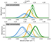 |
Fig. 10. Three Gaussian distributions plotted from 10 K to 170 K, for a low and high CO2 concentration in the ice. Blue represents |


Furthermore, we explored the influence of deposition pressure on the band positions. To investigate this aspect, an experiment was conducted with a deposition pressure of 8 × 10⁻⁷ mbar and a 4% CO2 concentration. Upon analyzing the band positions at 10 K, it was observed that the positions of  (2345 cm−1, 4.26 μm) and
  (2341 cm−1, 4.27 μm) were consistent with the experiment conducted at a lower deposition pressure. The higher deposition pressure is known to induce changes in the ice morphology, rendering it more porous (Maté et al. 2008; Bossa et al. 2015). The DFT simulations detailed in Sect. 7 show the effect porosity has on amorphous CO2 ice, allowing the CO2 dangling bond to occur. As the ice produced at higher pressure is more porous, it undergoes greater reorganization during the warm-up process. At 10 K,
  has a small ∼1 cm−1 blue shift compared to the low deposition pressure. When the temperature reached 50 K, CO2 became crystalline and the reorganization was complete. At this point,
  ,
,  , and
, and  were all peaking at approximately 2349.8 cm−1 (4.256 μm), 2344.5 cm−1 (4.265 μm), and 2340.6 cm−1 (4.272 μm), respectively. These band positions are similar to the low deposition pressure experiment. The assignment of the different band components is discussed in the remainder of this section. As previously mentioned, when CO2 is mixed with water, three distinct peaks emerge.
The  band found at approximately 2345 cm−1 (4.26 μm) can be attributed to bulk CO2 ice. This is corroborated by the desorption temperature of pure CO2, which falls in the range of 80−85 K for both low and high CO2 concentrations. This desorption is illustrated in Fig. 4, with band positions shown in Table 2. This band is also referred to as the CO2-ext where the interaction with water is quite weak as expected if CO2 is superficially adsorbed, as proposed by Gálvez et al. (2007).
The  band arises when CO2 is mixed with water and peaks around 2340 cm−1 (4.27 μm). This band is the consequence of CO2 molecules interacting with the water ice matrix. This peak is also referred to as CO2-int in previous work (Gálvez et al. 2007; Maté et al. 2008), where individual CO2 molecules are trapped in the amorphous water ice and this interaction results in a slight weakening of the C-O bond, which produces a redshift on the IR spectrum (Sandford & Allamandola 1990). When increasing the temperature the integrated absorbance area of
  near 2340 cm−1 (4.27 μm) diminishes as the water ice evolves to a hexagonal structure and the CO2 molecules desorb from the water ice matrix.
Here,  was found at approximately 2351 cm−1 (4.254 μm) for low CO2 concentration and around 2353 cm−1 (4.250 μm) for high concentration. This band is present in pure CO2 ice, meaning that it is not caused by the interaction with water but is instead a consequence of the morphology of the ice. The band has been previously observed in ice growth experiments with high deposition rates (Gálvez et al. 2008), although it was not observable at lower deposition rates (Falk 1987). We propose that this band is caused by pores in the ice where the binding is particularly weak, as it occurs on the top surface of the ice, and the CO2 molecules are dangling from the pore surface. This preliminary assignment is supported by a vibrational mode that is connected to porosity, namely, a degree of freedom to vibrate that is not allowed in a compact CO2 ice structure; furthermore, the 2351 cm−1 position relative to that of the fundamental C=O stretch in CO2 ice is analogous to the relative position of the O-H dangling with respect to the O-H stretch in water ice (Matsuda et al. 2018). This phenomenon is further supported by the discussion in Sect. 7. Therefore, we assigned
  to the CO2 dangling bonds. When CO2 is mixed with water, this peak is also present; however, in this case, it remains above the 80 K temperature, which implies that following the desorption of bulk CO2 ice, carbon dioxide molecules can remain trapped in the pores of the amorphous solid water.
A similar explanation for this band location, involving molecules bonded to -OH dangling bonds in the water ice, was suggested by Matsuda et al. (2018) for CO molecules. In that case, two bands are assigned, namely CO molecules interacting with the OH dangling groups (CO-dangling OH) and CO molecules interacting with the oxygen atoms of the surface water molecules (CO-bonded OH). It was found that the area of the CO-dangling band increases when cycling to higher temperatures, meaning that CO molecules partially diffuse to CO-dangling OH groups on the surface of the amorphous water ice pores.
The position of this band, blueshifted from the pure CO2 stretching band, could be easily confused with a similar band observed in clathrate hydrates (Dartois & Schmitt 2009). In our case we can discard these cage-like structures as they are normally formed at much slower deposition rates and higher temperatures.
Other proposed explanations for this band location is that carbon dioxide is in a “complexed” form with water, as suggested by Chaban et al. (2007). A blue shift of 5 cm−1 compared to the pure CO2 ice is observed when bonded with one water molecule, and 10 cm−1 with two. Furthermore, the symmetric O-H stretching band undergoes a redshift when complexed with two water molecules and the intensity increases significantly. In this work, for a 4% CO2 concentration, there was no increase in intensity nor a redshift at 10 K for the symmetric O-H stretching band when compared to that of a pure H2O ice, ruling out the possibility of a complexed CO2.
7. Assignment of ν3.1 with DFT calculations
In order to better understand the influence of porosity in amorphous CO2, simulations were carried out using density functional theory (DFT; Hohenberg & Kohn 1964; Kohn & Sham 1965) using the CASTEP program (Clark et al. 2005) for geometry optimization and vibrational spectrum prediction.
Starting with a CO2 crystal, the amorphous ice models are created by applying temperature using molecular dynamics (MD) in the NPT ensemble until the structure melts. This was done with the Andersen barostat (Andersen 1980) at constant pressure and the Nose thermostat (Martyna et al. 1992) at rising temperatures. The porous model is then formed by removing CO2 molecules from the amorphous model’s core. DFT was then used to geometrically optimize the systems using the generalized gradient approximation (GGA) and functionals by Perdew-Burke-Ernzerhof (PBE). Infrared spectra were simulated using density functional perturbation theory (Refson et al. 2006) based on these improved models.
The calculated spectra are not intended to perfectly duplicate the measured wavenumbers for vibrational bands, but should be near within a margin of error. Most significantly, they are repeatable and can aid in understanding the influence of experimentally uncontrollable factors.
The simulated IR spectra of an amorphous CO2 model (blue line) and a porous CO2 model (orange line) are shown in Fig. 11. The morphology of the bulk ice model (right) and the porous model (left) are included for comparison. In the case of the bulk amorphous ice, we can see that the spectrum is very similar to the experimental case, with some expected offset for the wavenumber. In the porous model there is a clear blueshift of appproximately 4 cm−1 for the main peak. Most importantly, a new secondary peak emerges at higher wavenumbers. This pattern is very similar to the spectra seen in laboratory ice, as well as the recent observations of this same CO2 band in Ganymede. It must be stressed that the goal of this simulation is to simulate the effect of porosity on the peak location and shape. Therefore, finding the mechanism behind the shift rather than matching perfectly the band location with the same wavenumbers.
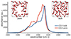 |
Fig. 11. DFT calculated spectra for bulk amorphous CO2 ice (blue) and a simulated pore in the same system (orange) as a function of wavenumber. |
8. Applications to icy moons
In this section, we use JWST ERS data from Ganymede (Bockelée-Morvan et al. 2024) and Europa (Villanueva et al. 2023) to study the position and evolution of the CO2 bands with varying latitude and longitude. The data were reprocessed from the Mikulski Archive for Space Telescopes (MAST) as described in Bockelée-Morvan et al. (2024). Our goal is to assign the CO2 bands observed to the physical state of CO2 ice. On Ganymede, the amount of CO2 relative to water in mass is of the order of 1% (Bockelée-Morvan et al. 2024), which implies that our low concentration experiments are more representative of these icy moons’ surfaces.
8.1. Ganymede
This section offers a discussion of the latitude and longitudinal spectra of Ganymede’s leading hemisphere, as similar trends are observed on the trailing hemisphere.
Figure 12 shows the CO2 band observed with JWST NIRspec on Ganymede as a function of latitude. The solid lines are JWST spectra and the colours indicate different latitudinal ranges, in good agreement with Bockelée-Morvan et al. (2024). The latitudinal variations of the CO2 band and its asymmetric band shape support the view that different CO2 ice physical states are involved. The 2342 cm−1 (4.27 μm) peak is stronger across the northern latitudes, which are colder and more enriched in water ice (Bockelée-Morvan et al. 2024; Trumbo et al. 2023). Across the equatorial latitudes, the 2353 cm−1 (4.25 μm) band becomes stronger. Ganymede has an average surface temperature around 100 K, with a maximum of 160 K at the equator (Bockelée-Morvan et al. 2024). Each latitude spectrum can be deconvolved into two Gaussian distribution that are represented with dotted lines and plotted for each range of latitudes. When analyzing the results, we can see that one of the Gaussians is located at 2341.7 cm−1 (4.270 μm) at the poles and shifts to lower wavelengths for other regions (supposedly warmer). This is in agreement with the  band observed experimentally, attributed to CO2 interacting with H2O molecules in the ice, which shifts slightly to the blue as the temperature increases. Moving closer to the equator, this peak shifts even more to the blue, reaching its maximum at 2342.5 cm−1 (4.269 μm). The second Gaussian is located around 2350.3 cm−1 (4.255 μm) at the North pole and around 2350.9 cm−1 (4.254 μm) at other latitudes. This is also in agreement with the
  band observed experimentally, which is blue-shifting from temperature above 150 K, which coincides with the surface temperature at Ganymede’s equator. In line with the experimental results, the presence of the
  band is identified as CO2 dangling bonds, which are an indication of ice porosity.
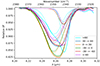 |
Fig. 12. Latitude spectra of Ganymede’s leading hemisphere acquired with JWST. Colours are used to indicate different latitude ranges. The dotted lines represent the Gaussian fit of each individual spectrum which is deconvolved in two Gaussians. |
The longitudinal spectra for Ganymede’s leading hemisphere are shown in Fig. 13. The solid lines are JWST spectra and the colours indicate different longitudinal ranges. The variations among the CO2 band position and intensity are shown in the figure for latitudes between 60° north and 60° south. The morning limb is represented by the 120−150 W spectrum (blue), whereas the evening limb is represented by the 30−60 W spectrum (red). Each spectrum is deconvolved into two Gaussian distributions, which are shown by dotted lines. The band at 2351 cm−1 (4.25 μm) has been assigned to the  band being an indication of the CO2 dangling bonds and of porosity. When comparing morning (blue) to evening (red), the
  band increases, suggesting that porosity increases during a day on Ganymede. This increase in porosity could be attributed to cracks in the ice that are forming due to temperature fluctuations. The effect of UV irradiation could also play an important role in this change in porosity that should also be considered.
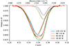 |
Fig. 13. Longitudinal spectra of Ganymede’s leading hemisphere acquired with JWST. The longitudes are taken between 60° North and 60° South in latitude. The spectrum for 120−150 W represents the morning limb of the leading edge and the evening limb by the 30−60 W spectrum. Colors are used to indicate different longitudinal ranges. The dotted lines represent the Gaussian fit of each individual spectrum which is deconvolved into two Gaussians. |
8.2. Europa
Figure 14 shows the CO2 band observed on Europa as a function of the latitude and exhibits similar variation as that reported by Villanueva et al. (2023). The band ca. 2342 cm−1 (4.27 μm) is stronger across the northern latitudes, which are colder and more enriched in water ice (Trumbo & Brown 2023). Across the equatorial latitudes, the 2353 cm−1 (4.25 μm) peak becomes stronger. The temperature on Europa ranges from 60 K at the poles to around 110 K at the equator, which is colder than on Ganymede. The Gaussian fits of the data are represented with dotted lines, and plotted for each range of latitudes. Each latitude spectrum can be deconvolved into two Gaussian distributions (as seen in Fig. 14). The band around 2342 cm−1 (4.27 μm) feature shifts when moving closer to the equator, from 2340.9 cm−1 (4.272 μm) for 30° to 60° North to 2341.2 cm−1 (4.271 μm) at the equator. This is in agreement with the  band position observed experimentally, which is located around 2340.8 cm−1 (4.272 μm) and shifts to the blue with increasing temperatures. The second Gaussian
  , located at 2353.5 cm−1 (4.249 μm), is shifted to the blue by around 3 cm−1 when compared to Ganymede. This is consistent with our experimental results showing the
  band shifts to higher wavelength with decreasing temperature.
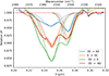 |
Fig. 14. Latitude spectra of Europa’s leading hemisphere acquired with JWST. Colours are used to indicate different latitude ranges. The dotted lines represent the Gaussian fit of each individual spectrum, each consisting of two Gaussians. |
The main conclusion of this section is that CO2 observations of both Ganymede and Europa can be explained by the presence of two components, the  band and
  band. The
  band located at 2342 cm−1 (4.27 μm) represents CO2 trapped in water ice and can account for the CO2 band observed in Ganymede’s and Europa’s spectra of the leading hemisphere, and is stronger in the boreal regions especially for Ganymede. The
  band at 2353 cm−1 (4.25 μm) for Europa and at 2350.9 cm−1 (4.254 μm) for Ganymede is stronger in other regions for both Ganymede and Europa. This band is associated with CO2 dangling bonds which depend on the pores present in the ice, as CO2 molecules on the pore walls can exhibit such dangling bonds. The band assignment of
  to CO2 in pores has been suggested, based on our experimental data combined with DFT simulations. It should be noted that the 2353 cm−1 (4.25 μm) band depends on the concentration of CO2 in the water ice, which will make the band shift.
9. Conclusions
In this study, we combined FTIR measurements and TPD experiments to explain the complexity of the CO2 stretching band. The examination of CO2 ice behaviour on icy moons has offered intriguing revelations about its interaction within these distinct environments. Moreover, aligning laboratory findings and DFT calculations with JWST data from Ganymede and Europa, bridges the gap between theory, experiments, and celestial icy surfaces. These findings can help enrich our understanding of these moons’ environments.
-
The C–O stretching band observed for pure CO2 ice at 10 K consists of two distinct vibrations:
 which is caused by porosity and peaks at 2351.3 cm−1 (4.253 μm), and
  which corresponds to bulk CO2 ice and peaks at 2345 cm−1 (4.264 μm). The band’s shape evolves during warm-up from 10 K to 80 K, exhibiting a redshift in both Gaussians. The TPD data indicates a desorption peak at 85 K, suggesting a thermal desorption of CO2 from the ice layer.
 -
CO2 mixed with water ice (at low and high concentration) exhibits multiple peaks, of which two are the same as for pure CO2. The presence of three peaks,
 at 2351 cm−1 (4.25 μm),
  at 2345 cm−1 (4.26 μm), and
  at 2341 cm−1 (4.27 μm) at 10 K demonstrates the complexity of CO2 interaction within water ice. The different CO2 bands are assigned as follows:
  (2351 cm−1, 4.25 μm) is associated to CO2 dangling bonds in which CO2 molecules are found in pores or cracks,
  (2345 cm−1, 4.26 μm) is due to CO2 trapped in the water ice (segregated) forming pockets of pure CO2, and
  (2341 cm−1, 4.27 μm) is related to CO2 molecules embedded in the ice interacting with water molecules.
 -
Thermal desorption analysis allowed for distinct peaks in the desorption curves to be assigned, indicating different desorption behaviours for CO2 within the ice. The low and high concentrations display similar desorption patterns. Initial CO2 desorption occurs around 80 K, followed by peaks at 146 K and 162 K, indicating various CO2-water interactions during ice phase transitions. Continuous desorption between 80 and 146 K is observed, driven by the amorphous water ice rearrangement and thereby facilitating CO2 diffusion through pores in the ice matrix.
-
The JWST NIRSPEC spectra of Ganymede’s leading hemisphere reveals significant variations in the CO2 band profile across different latitudes. Two main CO2 bands have been observed, that we assigned to
 (2353 cm−1, 4.25 μm) and
  (2342 cm−1, 4.27 μm). The dominance of
  (2353 cm−1, 4.25 μm) in northern latitudes, associated with colder regions enriched in water ice, is in contrast with the prevalence of
  (2342 cm−1, 4.27 μm) in equatorial latitudes. Gaussian fits of the spectra suggest two distinct physical states of CO2 that shift with temperature, which confirm the assignments from our laboratory findings. The CO2 band shifts observed on Ganymede with latitude could be attributed to an increase in temperature, showing that in the poles CO2 is well embedded in water ice.
 -
The longitudinal spectra for Ganymede’s leading hemisphere indicates variations in CO2 spectra from morning to evening. The band is assigned to the
 band (2351 cm−1, 4.25 μm) that links to the porosity of the ice. This increase in porosity could be attributed to cracks created in the ice due to variation of temperatures.
Similarly, the JWST NIRSPEC spectra of Europa’s leading hemisphere can be deconvolved into two Gaussian fits:  (2342 cm−1, 4.27 μm) assigned to CO2 molecules trapped in the water ice and
  (2353 cm−1, 4.25 μm) assigned to dangling CO2 molecules in pores or cracks. Temperatures in Europa are colder than Ganymede and as expected show a blueshift for
  and a redshift for
  when compared to the warmer moon. A similar effect is observed when comparing spectra from the warmer equator to the colder poles, indicating higher porosity near the equator.
Acknowledgments
The authors would like to thank I. de Pater, T. Fouchet, and D. Bockelée-Morvan for the use of the JWST ERS Ganymede data and assistance with processing, as well as G. Villanueva for the use of the JWST Europa data. This research has been funded by project PID2020-118974GB-C21 by the Spanish Ministry of Science and Innovation. B.E. acknowledges support by grant PTA2020-018247-I by the Spanish Ministry of Science and Innovation/State Agency of Research MCIN/AEI.
References
- Andersen, H. C. 1980, J. Chem. Phys., 71, 2384 [NASA ADS] [CrossRef] [Google Scholar]
- Bernstein, M. P., Cruikshank, D. P., & Sandford, S. A. 2005, Icarus, 179, 527 [NASA ADS] [CrossRef] [Google Scholar]
- Bockelée-Morvan, D., Lellouch, E., Poch, O., et al. 2024, A&A, 681, A27 [NASA ADS] [CrossRef] [EDP Sciences] [Google Scholar]
- Bossa, J.-B., Maté, B., Fransen, C., et al. 2015, ApJ, 814, 47 [NASA ADS] [CrossRef] [Google Scholar]
- Bouilloud, M., Fray, N., Bénilan, Y., et al. 2015, MNRAS, 451, 2145 [Google Scholar]
- Buratti, B., Cruikshank, D. P., Brown, R. H., et al. 2005, ApJ, 622, L149 [NASA ADS] [CrossRef] [Google Scholar]
- Cazaux, S., Bossa, J.-B., Linnartz, H., & Tielens, A. 2015, A&A, 573, A16 [NASA ADS] [CrossRef] [EDP Sciences] [Google Scholar]
- Chaban, G. M., Bernstein, M., & Cruikshank, D. P. 2007, Icarus, 187, 592 [NASA ADS] [CrossRef] [Google Scholar]
- Clark, S. J., Segall, M. D., Pickard, C. J., et al. 2005, Z. Kristall., 220, 567 [NASA ADS] [Google Scholar]
- Crovisier, J. 2006a, Mol. Phys., 104, 2737 [NASA ADS] [CrossRef] [Google Scholar]
- Crovisier, J. 2006b, Faraday Discuss., 133, 375 [NASA ADS] [CrossRef] [Google Scholar]
- Dartois, E., & Schmitt, B. 2009, A&A, 504, 869 [NASA ADS] [CrossRef] [EDP Sciences] [Google Scholar]
- Dartois, E., Pontoppidan, K., Thi, W.-F., & Caro, G. M. 2005, A&A, 444, L57 [NASA ADS] [CrossRef] [EDP Sciences] [Google Scholar]
- Draine, B. T. 2003, ARA&A, 41, 241 [NASA ADS] [CrossRef] [Google Scholar]
- Ehrenfreund, P., Boogert, A., Gerakines, P., Tielens, A., & Van Dishoeck, E. 1997, A&A, 328, 649 [NASA ADS] [Google Scholar]
- Falk, M. 1987, J. Chem. Phys., 86, 560 [NASA ADS] [CrossRef] [Google Scholar]
- Gálvez, O., Ortega, I. K., Maté, B., et al. 2007, A&A, 472, 691 [NASA ADS] [CrossRef] [EDP Sciences] [Google Scholar]
- Gálvez, O., Maté, B., Herrero, V. J., & Escribano, R. 2008, Icarus, 197, 599 [CrossRef] [Google Scholar]
- Gerakines, P. A., Schutte, W. A., Greenberg, J. M., & van Dishoeck, E. F. 1995, A&A, 296, 810 [NASA ADS] [Google Scholar]
- González Díaz, C., Carrascosa, H., Muñoz Caro, G. M., Satorre, M., & Chen, Y.-J. 2022, MNRAS, 517, 5744 [CrossRef] [Google Scholar]
- Grundy, W., Young, L., & Young, E. 2003, Icarus, 162, 222 [NASA ADS] [CrossRef] [Google Scholar]
- Hagen, W., Tielens, A., & Greenberg, 1981, J. Chem. Phys., 56, 367 [NASA ADS] [Google Scholar]
- Hansen, G. B., & McCord, T. B. 2008, Geophys. Res. Lett., 35, L01202 [NASA ADS] [CrossRef] [Google Scholar]
- Hohenberg, P., & Kohn, W. 1964, Phys. Rev., 136, B864 [CrossRef] [Google Scholar]
- Isokoski, K., Poteet, C., & Linnartz, H. 2013, A&A, 555, A85 [NASA ADS] [CrossRef] [EDP Sciences] [Google Scholar]
- Kohn, W., & Sham, L. J. 1965, Phys. Rev., 140, A1133 [CrossRef] [Google Scholar]
- Kumi, G., Malyk, S., Hawkins, S., Reisler, H., & Wittig, C. 2006, J. Phys. Chem. A, 110, 2097 [NASA ADS] [CrossRef] [Google Scholar]
- Malyk, S., Kumi, G., Reisler, H., & Wittig, C. 2007, J. Phys. Chem. A, 111, 13365 [NASA ADS] [CrossRef] [Google Scholar]
- Martín-Doménech, R., Caro, G. M., Bueno, J., & Goesmann, F. 2014, A&A, 564, A8 [NASA ADS] [CrossRef] [EDP Sciences] [Google Scholar]
- Martyna, G. L., Klein, M. L., & Tuckerman, M. 1992, J. Chem. Phys., 97, 2635 [NASA ADS] [CrossRef] [Google Scholar]
- Maté, B., Gálvez, O., Martín-Llorente, B., et al. 2008, J. Phys. Chem. A, 112, 457 [CrossRef] [Google Scholar]
- Matsuda, S., Yamazaki, M., Harata, A., & Yabushita, A. 2018, Chem. Lett., 47, 468 [Google Scholar]
- McCord, T. B., Hansen, G. B., Clark, R. N., et al. 1998, J. Geophys. Res., 103, 8603 [NASA ADS] [CrossRef] [Google Scholar]
- Mishra, I., Lewis, N., Lunine, J., et al. 2021, Planet. Sci. J., 2, 183 [NASA ADS] [CrossRef] [Google Scholar]
- Muñoz Caro, G., Jiménez-Escobar, A., Martín-Gago, J., et al. 2010, A&A, 522, A108 [NASA ADS] [CrossRef] [EDP Sciences] [Google Scholar]
- Refson, K., Tulip, P. R., & Clark, S. J. 2006, Phys. Rev. B, 73, 155114 [NASA ADS] [CrossRef] [Google Scholar]
- Sandford, S., & Allamandola, L. 1990, ApJ, 355, 357 [NASA ADS] [CrossRef] [Google Scholar]
- Trumbo, S. K., & Brown, M. E. 2023, Science, 381, 1308 [NASA ADS] [CrossRef] [Google Scholar]
- Trumbo, S. K., Brown, M. E., Bockelée-Morvan, D., et al. 2023, Sci. Adv., 9, eadg3724 [NASA ADS] [CrossRef] [Google Scholar]
- Villanueva, G., Hammel, H., Milam, S., et al. 2023, Science, 381, 1305 [NASA ADS] [CrossRef] [Google Scholar]
All Tables
All Figures
|
Fig. 1. ISAC cross-section at the ice sample level. The measuring devices and sensors, including the laser interferometry, are displayed. The FTIR source is positioned on one side and the FTIR detector on the opposite one. The UV spectrometer is placed directly across from the vacuum-UV lamp, see González Díaz et al. (2022) for more details. |
| In the text | |
|
Fig. 2. Spectra over the 2380−2320 cm−1 (4.20−4.31 μm) range of a pure CO2 ice deposited at 10 K and 2 × 10⁻⁷ mbar, later warmed up to 90 K. All spectra are measured at 2 cm−1 resolution, and at temperatures indicated in each graph. Spectra are shifted vertically for clarity. |
| In the text | |
|
Fig. 3. Evolution of both Gaussian distributions during warm-up from 10 K to 80 K for a pure CO2 ice. The arrows indicate the direction of evolution. Thicker lines indicate the initial and final states. |
| In the text | |
|
Fig. 4. TPD curve of pure CO2 ice layer deposited at 10 K and heated at 0.5 K/min. The ion current (A) is plotted on a logarithmic scale for a better appreciation of the curve profile and roughly corresponds to partial pressure in mbar. |
| In the text | |
|
Fig. 5. Column density of CO2 ice (triangles) calculated from IR measurements matches the calculated coverage (light blue line). TPD curve of CO2 from QMS measurements (dark blue) agrees well with the fit corresponding to the Polanyi-Wigner equation (red line). |
| In the text | |
|
Fig. 6. Spectra over the 2380−2320 cm−1 (4.20−4.31 μm) range of the H2O:CO2 = 1:0.04 ice mixture deposited at 10 K and 2 × 10⁻⁷ mbar. All spectra are measured with 2 cm−1 resolution at the temperatures indicated in each graph. Spectra are shifted vertically for clarity. |
| In the text | |
|
Fig. 7. TPD curves of CO2 and H2O for a H2O:CO2 = 1:0.04 ice heated at 0.2 K/min (top). Integrated absorbance areas of the three Gaussian distributions as a function of temperature for the same experiment (bottom). |
| In the text | |
|
Fig. 8. Spectra over the 2380−2320 cm−1 (4.20−4.31 μm) range of the H2O:CO2 = 1:0.25 ice mixture deposited at 10 K and 2 × 10⁻⁷ mbar. All spectra are measured with 2 cm−1 resolution at the temperatures indicated in each graph. Spectra are shifted vertically for clarity. |
| In the text | |
|
Fig. 9. TPD curves of CO2 and H2O for a H2O:CO2 = 1:0.25 ice layer heated at 0.2 K/min (top). Integrated absorbance areas of the three Gaussian distributions as a function of temperature for a H2O:CO2 = 1:0.25 ice (bottom). |
| In the text | |
|
Fig. 10. Three Gaussian distributions plotted from 10 K to 170 K, for a low and high CO2 concentration in the ice. Blue represents |
| In the text | |
|
Fig. 11. DFT calculated spectra for bulk amorphous CO2 ice (blue) and a simulated pore in the same system (orange) as a function of wavenumber. |
| In the text | |
|
Fig. 12. Latitude spectra of Ganymede’s leading hemisphere acquired with JWST. Colours are used to indicate different latitude ranges. The dotted lines represent the Gaussian fit of each individual spectrum which is deconvolved in two Gaussians. |
| In the text | |
|
Fig. 13. Longitudinal spectra of Ganymede’s leading hemisphere acquired with JWST. The longitudes are taken between 60° North and 60° South in latitude. The spectrum for 120−150 W represents the morning limb of the leading edge and the evening limb by the 30−60 W spectrum. Colors are used to indicate different longitudinal ranges. The dotted lines represent the Gaussian fit of each individual spectrum which is deconvolved into two Gaussians. |
| In the text | |
|
Fig. 14. Latitude spectra of Europa’s leading hemisphere acquired with JWST. Colours are used to indicate different latitude ranges. The dotted lines represent the Gaussian fit of each individual spectrum, each consisting of two Gaussians. |
| In the text | |
Current usage metrics show cumulative count of Article Views (full-text article views including HTML views, PDF and ePub downloads, according to the available data) and Abstracts Views on Vision4Press platform.
Data correspond to usage on the plateform after 2015. The current usage metrics is available 48-96 hours after online publication and is updated daily on week days.
Initial download of the metrics may take a while.