© The Authors 2024

1. Introduction

A galactic bar is a linear elongated stellar structure spanning the center of a disk galaxy. In the local Universe, ∼70% of the disk galaxies host a bar when viewed in optical or near-infrared (NIR) wavelengths (e.g. Menéndez-Delmestre et al. 2007; Marinova & Jogee 2007; Aguerri et al. 2009; Ho et al. 2011; Buta et al. 2015; Erwin 2018; Yu et al. 2022a). The bar fraction may vary with Hubble types, stellar mass, and color index (Nair & Abraham 2010; Barazza et al. 2008; Díaz-García et al. 2016; Erwin 2018). It is generally accepted that stellar bars play an important role in galaxy evolution. The nonaxisymmetric bar gravitational potential drives cold gas flow toward the galaxy center along the dust lane of the bar, enhancing central star formation and leading to the growth of pseudo-bulges (Athanassoula 1992, 2002; Athanassoula et al. 2005; Kormendy & Kennicutt 2004; Jogee et al. 2005; Ellison et al. 2011; Wang et al. 2012, 2020; Gadotti et al. 2020; Yu et al. 2022a,b). In addition, bars reshape the galaxy morphology by rearranging the mass distribution and by forming substructures such as disk break, spiral arms, and rings (e.g., Knapen et al. 1995; Kormendy & Kennicutt 2004; Ellison et al. 2011; Erwin & Debattista 2013; Gadotti et al. 2020).

Through observations from the Hubble Space Telescope (HST), the bar fraction is found to evolve with redshift. Early HST study by Abraham et al. (1999) reported a decline in the bar fraction toward higher redshifts (see also Abraham et al. 1996; van den Bergh et al. 1996), while Elmegreen et al. (2004) and Jogee et al. (2004) later found that the bar fraction remains consistent up to z ≈ 1. With a dataset of a considerably large sample covering a wide mass range, Sheth et al. (2008) demonstrated that the bar fraction decreases from 65% at z = 0.2 to 20% at z = 0.84 (see also Cameron et al. 2010). The declining trend was further confirmed by Melvin et al. (2014) using visual classifications from the Galaxy Zoo (Willett et al. 2013). By studying barred galaxies at 0.2 < z ≤ 0.835, Kim et al. (2021) found that normalized bar sizes do not exhibit any clear cosmic evolution, implying that bar and disk evolution are closely intertwined throughout time. Simulation work by Kraljic et al. (2012) showed that the bar fraction drops to nearly zero at z ≈ 1, suggesting that bars provide a tool for identifying the transition epoch between the high-redshift merger-dominated or turbulence-dominated disks and local dynamically settled disks. Nevertheless, a recent study of IllustrisTNG galaxies found that the bars appear as early as at z = 4 and that the bar fraction evolves mildly with cosmic time (Rosas-Guevara et al. 2022). The authors argued that when long bars are considered alone, their results can be reconciled with those from observational studies because they can suffer from resolution effects.

The analysis of bar structures in galaxies at high redshift using HST observations presents a considerable challenge. For galaxies at z ≳ 2, imaging through the HST F814W filter observes the rest-frame ultraviolet, at which wavelength, bars are often poorly visible (Sheth et al. 2003). The HST NIR F160W imaging has a relatively broader point spread function (PSF), with which bar structures at high redshift can be resolved only inadequately. In addition, the depth of HST observations might be insufficient for detecting the outer regions of high-redshift galaxies, causing galaxies with a long bar to resemble edge-on galaxies. The James Webb Space Telescope (JWST) delivers images with unparalleled sensitivity and resolution in the NIR, which significantly enhances our understanding of galaxy structures at high redshift. Recent JWST studies have revealed a significant fraction of regular disk galaxies at high redshift (Ferreira et al. 2022, 2023; Kartaltepe et al. 2023; Nelson et al. 2023; Robertson et al. 2023; Jacobs et al. 2023; Xu & Yu 2024). This result contrasts with the findings from HST-based studies, which predominantly identified peculiar galaxies at z > 2 (e.g., Conselice et al. 2008; Mortlock et al. 2013). Remarkably, barred galaxies at z ≈ 2–3, previously undetected in HST observations, have now been identified using the JWST (Guo et al. 2023; Le Conte et al. 2024; Costantin et al. 2023).

Although JWST imaging offers exceptional angular resolution, its physical resolution when observing high-redshift galaxies is still lower than that achieved with ground-based observations of nearby galaxies. This complicates direct comparisons between bars observed in low-redshift and high-redshift galaxies, making the study of bar evolution less straightforward. Sheth et al. (2003) pointed out that the bar fraction calculated using low-resolution images tends to be underestimated. This underestimation is likely to be exacerbated by the bar size evolution, wherein bars become shorter in physical size at higher redshift, as predicted in numerical simulations (e.g., Debattista & Sellwood 2000; Martinez-Valpuesta et al. 2006; Athanassoula 2013; Algorry et al. 2017). In contrast, the influence of cosmological surface brightness dimming on bar detection is minimal (Sheth et al. 2008). By analyzing apparent bar sizes in galaxies from the Spitzer Survey of Stellar Structure in Galaxies (S⁴G; Sheth et al. 2010, Erwin 2018) showed that most of the projected bar radii are larger than twice the PSF full width at half-maximum (FWHM), and the authors thus suggested this value as the bar detection threshold. This threshold successfully reconciles the difference in the dependence of the bar fraction on parameters such as stellar mass or gas fraction, especially when their results are compared with studies based on low-resolution SDSS images (Masters et al. 2012; Oh et al. 2012; Melvin et al. 2014; Gavazzi et al. 2015). Likewise, based on extensive experiments on artificial galaxies, Aguerri et al. (2009) suggested that the limitation of the bar detection is 2.5 times the FWHM. Nevertheless, the threshold bar size for a bar detection has not yet been validated in a quantitative way based on real images, especially under typical JWST observational conditions. The resolution may also impact measured bar properties such as size, ellipticity, and position angle, which are frequently employed to study the formation and evolution of bars (e.g., Elmegreen et al. 2007; Gadotti 2011; Kim et al. 2021; Yu et al. 2022a). While it seems intuitive that the bar ellipticity would be underestimated due to PSF smoothing as spatial resolution deteriorates, the exact impact and the influence on other parameters remain largely unexplored.

It is therefore nontrivial to interpret the observational results obtained from JWST without knowing the systematics caused by the observation limitations. To disentangle the potential intrinsic relations or evolution for bars from the observation effects, we aim to understand here how the observational factors can influence the identification and quantification of bars. By accounting for observational effects and galaxy evolution, Yu et al. (2023) recently used a sample of nearby galaxies to create images of simulated high-redshift galaxies as they would be observed by JWST in the Cosmic Evolution Early Release Science (CEERS) survey (PI: Finkelstein, ID = 1345; Finkelstein et al. 2022; Bagley et al. 2023). In addition to the simulated galaxy CEERS images provided by Yu et al. (2023), we employ their sample of nearby galaxies to produce images at low resolution for a given signal-to-noise ratio (S/N) and at low S/N for a given resolution. We then compare the measurements before and after image degradation to understand how reliably bars in high-redshift galaxies observed with JWST can be analyzed. The structure of this paper is as follows. Section 2 presents an overview of the dataset. Section 3 describes the procedure for generating images mimicking the JWST resolution and S/N. In Sect. 4, we present the robustness of the bar structure measurements for JWST observations. We discuss the implication of our results in Sect. 5. A summary is given in Sect. 6. Throughout this work, we use AB magnitudes and assume Ω_M = 0.27, Ω_Λ = 0.73, and h = 0.70.

2. Observational material

We constructed the sample based on which we studied how reliably bars can be identified and quantified based on the nearby galaxy sample defined in Yu et al. (2023). By a restriction to a luminosity distance (D_L) of 12.88 ≤ D_L ≤ 65.01 Mpc and a stellar mass (M_⋆) of 10^{9.75 − 11.25} M_⊙, and by excluding images that were severely contaminated by close sources, Yu et al. (2023) selected 1816 galaxies from the Siena Galaxy Atlas¹ (SGA; Moustakas et al. 2021), which is made up of 383 620 galaxies from the Dark Energy Spectroscopic Instrument (DESI) Legacy Imaging Surveys (Dey et al. 2019). Out of the 1816 galaxies, we selected 448 face-on spiral galaxies by requiring that the galaxies were available in the third Reference Catalog of Bright Galaxies (RC3; de Vaucouleurs et al. 1991) and had a Hubble type of T > 0.5 and an axis ratio of b/a > 0.5. We excluded S0s because they are much rarer at high redshift than in the local Universe (e.g., Postman et al. 2005; Desai et al. 2007; Cavanagh et al. 2023), their bars are significantly different from those in spirals (e.g., Aguerri et al. 2009; Buta et al. 2010; Díaz-García et al. 2016), and because it is challenging to distinguish them from Es when the image quality is limited. The median angular luminosity distance and the typical DESI r-band FWHM of our sample is 43 Mpc and 0.9 arcsec. Thus, the FWHM translates into a typical linear resolution of 0.2 kpc. When we consider the high quality of the linear resolution of the DESI images and the typical bar size range of 0.5 − 10 kpc found in nearby galaxies (Erwin 2005; Díaz-García et al. 2016), the bar structures are effectively spatially resolved in our nearby galaxy sample. We used the star-cleaned r-band images provided by Yu et al. (2023) for our analysis, as the NIRCam of JWST traces the rest-frame optical light at high redshift. The star-cleaned images are essential for the creation of images of the various resolution and S/N levels observed by JWST. These images were generated by replacing the flux emitted by sources other than the target galaxy with interpolated flux or flux in the rotational symmetric regions (for details, see Yu et al. 2023).

Several methods have been established to identify bars and measure their properties, including visual inspection (e.g., de Vaucouleurs et al. 1991; Nair & Abraham 2010; Herrera-Endoqui et al. 2015), an ellipse-fitting method (e.g., Menéndez-Delmestre et al. 2007; Marinova & Jogee 2007; Sheth et al. 2008; Yu & Ho 2020), a Fourier analysis (e.g., Ohta et al. 1990; Elmegreen & Elmegreen 1985; Aguerri et al. 1998), and two-dimensional decomposition (e.g., Gadotti 2009; Laurikainen et al. 2005; Salo et al. 2015). Limitations and potential uncertainties are always associated with these techniques, and no single method can guarantee perfect results (Athanassoula & Misiriotis 2002; Aguerri et al. 2009; Lee et al. 2019). We used the ellipse-fitting method to analyze the bars. The isophote ellipticity (ϵ) has been shown to increase with radius within regions dominated by bars, beyond which, ϵ would drop (Menéndez-Delmestre et al. 2007; Aguerri et al. 2009). However, in some barred galaxies, especially the SAB galaxies (which represent an intermediate class between spirals and those with strong bars), this drop in the ϵ profile can be absent because the bar is not strictly straight, which reduces the difference in ϵ between the bar and the underlying disk. Another point to consider is the observational effect. For galaxies observed at high redshift, the drop in the ϵ profile can be smoothed out by the PSF, as demonstrated in Sect. 3. Therefore, we adopted the strategy suggested by Erwin & Sparke (2003) to seek out peaks in the ϵ profile as a signature of bars or potential bar candidates. While this approach is effective, we opted not to account for possible twists in the position angle (PA) profile, but supplemented our approach with visual inspections to ascertain the presence of bars.

We used the ellipse task from photutils² twice for each image to fit the isophote. First, we set the center, ϵ, and PA as free parameters, and we then determined the galaxy center by averaging the centers of the resulting isophotes in the inner region. Second, we fixed the center to derive the profiles of ϵ and PA. For each ϵ profile, we selected the bar candidates by a search for local peaks greater than 0.1 in the ϵ profile. For each bar candidate, we visually confirmed whether it represented a bar instead of dust lanes, star-forming regions, or spiral arms. If one of the candidates was confirmed as a bar, the galaxy was classified as a barred galaxy, and the semi-major axis (SMA), ϵ, and PA corresponding to the selected peak (denoted as a_{bar,  true}, ϵ_{bar,  true}, and ${\mathrm{PA}}_{\mathrm{bar},\mathrm{true}}$, respectively) were taken as the measures of the bar properties. The subscript “true” is used to distinguish these values from those obtained by analyzing simulated degraded images in Sect. 3. The a_{bar,  true} describes the apparent bar size. For several galaxies where a bar is obvious by visual inspection, the ϵ profile does not exhibit a peak because the ellipticity of the bar is comparable to that of the disk. We manually determined the SMA that best characterizes the bar and subsequently estimated its properties. The remaining galaxies were classified as unbarred galaxies.

Out of 448 spiral galaxies, 304 were classified as barred, yielding a bar fraction of 68%. Although this is slightly lower, it is consistent with previous studies that identified bars through visual inspection (e.g., de Vaucouleurs et al. 1991; Marinova & Jogee 2007; Buta et al. 2015). This fraction is marginally higher than was found in some studies using the ellipse-fitting methods (e.g., Barazza et al. 2008; Aguerri et al. 2009) that missed barred galaxies, especially the SAB types, that do not exhibit a sudden drop in their ϵ profiles. This calculated bar fraction of 68% is denoted as f_{bar,  true}. Figure 1 summarizes the basic bar properties in our sample. The distribution of ϵ_{bar,  true} is shown in the left panel, and the relation between a_{bar,  true} and galaxy stellar mass is displayed in the right panel. Our sample covers a wide range of bars, with ϵ_{bar,  true} values spanning from 0.25 to 0.85 and a_{bar,  true} ranging from 0.3 to 10 kpc. We demonstrate that more massive galaxies have longer a_{bar,  true}, consistent with previous work (e.g. Díaz-García et al. 2016; Erwin 2019; Kim et al. 2021), although our analysis does not involve the deprojection process for the bars. We refer to the properties derived from DESI images as the true bar properties due to the high quality of the DESI images.

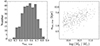Fig. 1. Basic properties of the barred galaxies in our sample. The left panel illustrates the distribution of the bar ellipticity (ϵbar,  true), and the right panel shows the projected bar size as semi-major axis (abar,  true) vs. stellar mass (M⋆).

3. Image simulations

Two approaches were employed to investigate the cosmological redshift effects on the detection and measurement of bars at high redshift with JWST. The first approach, to consider observational effects, was to use the r-band star-cleaned image of nearby galaxies to generate and study simulated images of various resolution and S/N (Sects. 3.1 and 3.2). In the second approach, we analyzed the simulated CEERS images that were created by taking observational effects and galaxy evolution into account (Sect. 3.3). We reidentified and remeasured the bars in these simulations to illustrate how resolution, noise, and their combined effects influence the analysis of bars in galaxies at high redshifts.

3.1. Simulated low-resolution images

The detectability of the bar is often gauged by the ratio of a_{bar,  true} to the PSF FWHM, that is, n = a_{bar,  true}/FWHM. The quantitative impact of this ratio remains to be elucidated, however. To observe the rest-frame optical wavelength, we assumed the F115W, F150W, and F200W filters to study bars in real observations at redshifts of z < 1, 1 ≤ z < 2, and 2 ≤ z < 3, respectively. Although the JWST F115W images can resolve bar structures better because their PSF is narrower, they may miss bars at high redshift due to the shift toward shorter rest-frame wavelengths. Consequently, the redder filters were used to mitigate this effect. We therefore examined three JWST PSFs corresponding to the filters F115W, F150W, and F200W, which had FWHMs of 0.037, 0.049, and 0.064 arcsec, respectively³. A pixel scale of 0.03 arcsec/pixel, consistent with the CEERS data release (Bagley et al. 2023), was adopted.

To generate low-resolution images for understanding the impact of PSF smoothing, we started by downsizing the star-cleaned images to match an exponentially increasing sequence of n values, 1.0, 1.2, 1.44, 1.73, 2.07, 2.49, 2.99, 3.58, 4.3, 5.16, and 10. Correspondingly, the DESI PSFs are resized using the same scaling factor. Next, we generated JWST PSFs using WebbPSF (Perrin et al. 2014) and derived a kernel via Fourier transformation to transform the resized PSF into the JWST PSF. Last, we convolved the downsized galaxy image with the kernel to obtain the simulated low-resolution image. These simulated images have a very high S/N, allowing us to focus on examining the impacts of the PSF. We analyzed the bar structure in each low-resolution image using the same ellipse-fitting method as outlined in Sect. 2. The derived bar size, ellipticity, and position angle are denoted $a_{\text{obs}}^n$, ${ϵ}_{\text{obs}}^n$, and ${\text{PA}}_{\text{obs}}^n$.

Figure 2 uses PGC049413 as an example to illustrate the impact of the decreasing resolution on the bar analysis for the F200W PSF. The images are shown in the left column, while the ϵ profiles are shown on the right. The top row shows the result derived from the DESI image. As the DESI image has a quite high resolution, indicated by a_{bar,  true}/FWHM = 19.02, there is clearly a bar in the image and a peak, or equivalently, a drop in the ϵ profile. The peak or the drop, marked by the solid line in the profile, was selected to measure the bar. An ellipse with the resulting parameters is overplotted on the image to illustrate the measurement. The subsequent rows present the results obtained from the simulated low-resolution images. To facilitate the comparison between the results before and after the resolution degradation, we adjusted the SMA of the DESI ϵ profile to match those from the low-resolution images, and we then plotted the adjusted profiles as dashed gray curves and the intrinsic bar size as the vertical dashed line. As the resolution decreases to a_{bar,  true}/FWHM = 5.16 and 3.58, the bar structures in the images remain clearly visible despite the increasing blur. The persistent peak in the ϵ profile underscores the presence of the bar, even though its amplitude decreases. This reduced peak amplitude indicates that the bar ellipticity is underestimated. In addition, the peak shifts inward, leading to an underestimation of measured bar size. Moreover, the sudden drop seen in the DESI ϵ profile softens at a_{bar,  true}/FWHM = 5.16 and is completely absent at a_{bar,  true}/FWHM = 3.58. This behavior caused us to use the peak in the ϵ profiles to identify bars, as described in Sect. 2. These changes in the image and the ϵ profiles are caused by the PSF convolution, which rounds the bar structure and reduces its clarity at the edges. When the resolution decreases to a_{bar,  true}/FWHM = 2.07, the image becomes more unclear, causing subtle structural details such as spiral arms to fade significantly. However, the bar structure remains discernible in the image, with a distinct peak in the ϵ profile. When the resolution further decreases to a_{bar,  true}/FWHM = 1, the image has become so blurred that no structure is visible any longer, and the characteristic features corresponding to a bar in the ϵ profile disappear.

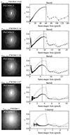Fig. 2. Impact of the decreasing resolution on the bar analysis, using PGC049413 as an example. On the left are the galaxy images, and their respective derived ϵ profiles are shown at the right. At the top of each image, the ratio of abar,  true to the FWHM is indicated. The first row shows the results from DESI, succeeded by the results from low-resolution F200W images in the rows below. The DESI ϵ profiles are plotted with dashed gray curves in the right panels. The intrinsic bar position is denoted as the vertical dashed gray line. When a bar is successfully identified, it is marked in the image by an ellipse and indicated in the profile by a vertical solid line.

For the simulated images of PGC049413, we note the significant decrease in the measured bar size. At a_{bar,  true}/FWHM = 3.58, the fractional difference between the measured and intrinsic bar size is −25%. However, these cases are not typical. A lower resolution only reduces the measured bar size by a few percent on average when a_bar/FWHM > 2, as we discussed in detail in Sect. 4. Figure 3 uses NGC0514, an SAB galaxy, as an example to illustrate the typical resolution effect. At a_{bar,  true}/FWHM = 4.3, the bar size still matches the original size, while at a_{bar,  true}/FWHM = 2.49, the observed bar size is reduced by 5%. However, at a_{bar,  true}/FWHM = 1.73, the bar size is overestimated because the image is blurred, causing part of the spiral structure to be recognized as the bar. At a_{bar,  true}/FWHM = 1.2, the bar structure is completely lost. Additionally, similar to the previous illustration of PGC049413, the amplitude of the ϵ profile gradually decreases as the resolution worsens.

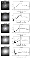Fig. 3. Impact of the decreasing resolution on the bar analysis, using NGC0514 as another example. The details are the same as in Fig. 2.

3.2. Simulated images with a low signal-to-noise ratio

To explore the influence of noise on the bar analysis under realistic observational conditions in CEERS, we first estimated the S/N range of the galaxy images observed in the survey. We used the science data, error map, and source mask from the CEERS Data Release Version 0.6 (for the data reduction, see Bagley et al. 2023)⁴. We used the catalog of Stefanon et al. (2017) to select galaxies with stellar mass M_⋆ ≥ 10^9.75 M_⊙ at redshifts of 0.75 ≤ z ≤ 3.0, and then used sep (Bertin & Arnouts 1996; Barbary 2016) to generate a mask for each galaxy. Images of galaxies that were severely contaminated by close sources were excluded. We calculated the sky uncertainty through Autoprof (Stone et al. 2021) and derived the galaxy flux uncertainty from the error map. We calculated the map of S/N for each galaxy by dividing the galaxy flux by the flux uncertainty pixel by pixel, and computed the average S/N over an elliptical aperture with SMA of the Petrosian galaxy radius, and with galaxy ϵ and PA. This average S/N value is considered as the S/N of this galaxy. The rationale for calculating the S/N averaged over the pixels occupied by the galaxy instead of simply dividing the total galaxy flux by its uncertainty (which treats the galaxy like a point source) is that the S/N of individual pixels can vary throughout the galaxy. Since bars are extended structures, averaging the S/N over the pixels that encompass the bars represents the signal strength of the bars relative to the noise better.

As a result, for CEERS galaxies observed in the F115W (0.75 < z < 1), F150W (1 < z < 2), and F200W (2 < z < 3) filters, the median S/N values are 20.0, 11.4, and 10.0, respectively. The corresponding standard deviations are 11.5, 9.5, and 9.0. Moreover, over 95% of galaxies in each filter exhibit an S/N greater than 3. Therefore, to investigate whether and how the typical noise level in CEERS influences our bar analysis, we used the high-S/N simulated image of a_{bar,  true}/FWHM = 4.3 to generate simulated images for each galaxy with an exponentially increasing S/N: 3, 4.2, 5.9, 8.2, 11.5, 16.1, 22.6, 31.6, 44.3, and 62.0. The ratio a_{bar,  true}/FWHM was fixed to isolate the noise effect. We verified that using images of other a_{bar,  true}/FWHM to examine noise effects does not affect our results significantly. To make the image noisy, we rescaled the image flux with a scaling factor, derived the flux noise, and added the flux noise as well as a background map to the flux-rescaled image. In this process, we used the median ratio of the galaxy flux to the flux variance and the patch of cleaned real CEERS background, as provided by Yu et al. (2023), to compute the galaxy flux noise and to represent the background map, respectively. The scaling factor was adjusted iteratively to match our desired S/N. We applied the same ellipse-fitting method as described in Sect. 2 to identify and quantify bars. The derived bar size, ellipticity, and position angle from these images of various S/N are denoted $a_{\mathrm{obs}}^{S/N}$, ${ϵ}_{\mathrm{obs}}^{S/N}$, and ${\mathrm{PA}}_{\mathrm{obs}}^{S/N}$.

With the layout consistent with Fig. 2, Fig. 4 uses PGC049413 as an example to illustrate the impact of noise. When S/N ≥ 16.1 (top four rows), noise hardly affects the images, keeping the bar structure clear and the corresponding ϵ profiles unchanged. As the S/N drops to 8.2 and further to 3 (bottom two rows), the influence of noise becomes slightly more significant, resulting in a decrease in image clarity and greater uncertainty in the ϵ profile. Despite this, the bar structure is still discernible, and the general shape of the ϵ profiles changes only little. The measurements of the bar size and ellipticity from images with low S/N are consistent with those from images with a high S/N. Therefore, the bar identification and quantification for PGC049413 are not significantly affected by the noise within the typical S/N range observed in the CEERS field.

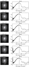Fig. 4. Impact of noise on the bar analysis. The symbols are the same as in Fig. 2. The top row now displays the noiseless simulated image of abar,  true/FWHM = 4.3 and its profile, and the subsequent rows show the simulated low-S/N images and their profiles.

3.3. Simulated galaxy images observed in CEERS

To examine the cosmological redshift effect, which is a combination of the resolution and noise effects in a specific way, simulated CEERS images in which both observational effects and evolution effects are considered are essential. Yu et al. (2023) used multiwaveband images of a sample of nearby DESI galaxies to generate artificially redshifted images observed in JWST CEERS at z = 0.75, 1.0, 1.25, 1.5, 1.75, 2.0, 2.25, 2.5, 2.75, and 3.0. The F115W filter was used for z = 0.75 and 1, the F150W filter was used for z = 1.25, 1.5, and 1.75, and the F200W filter was used for z = 2.0 to 3.0. Their image simulation procedure involved spectral change, cosmological surface brightness dimming, luminosity evolution, physical disk size evolution, shrinking in angular size due to distance, decrease in resolution, and increase in noise level (for details, see Yu et al. 2023). In particular, the PSFs were matched to those generated using WebbPSF, and a cleaned blank CEERS background was employed. A bar evolution model was incorporated. With increasing redshift, the physical size of the bars becomes shorter as the disk size becomes smaller, following the galaxy size evolution derived by van der Wel et al. (2014). Applying a galaxy evolution model is a separate consideration in addition to the basic resolution and S/N effects. This dataset fits our scientific goal of understanding the redshift effects on the bar measurements. We analyzed each simulated CEERS image using the ellipse-fitting method described in Sect. 2. The resultant bar size, ellipticity, and position angle are denoted $a_{\mathrm{obs}}^z$, ${ϵ}_{\mathrm{obs}}^z$, and ${\mathrm{PA}}_{\mathrm{obs}}^z$.

Figure 5 shows the redshift effects on the bar measurement. The top row displays the results derived from the DESI image, and the subsequent rows present the results from the simulated CEERS images at high redshifts. The galaxy structures in the DESI image are clear, and the drop or peak in the ϵ profile is prominent. When the galaxy is artificially moved to z = 1 and then further to z = 3, the galaxy image becomes increasingly blurred and noisy. The ϵ profiles tend to flatten, and the sudden drop in the ϵ profile disappears entirely at z ≥ 1.5. The flattening in the ϵ profiles is due to the decreasing a_{bar,  true}/FHWM with increasing redshift, consistent with the expectation based on the resolution effect discussed in Sect. 3.1. As anticipated from Sect. 3.2, the noise only causes the profiles at high redshift to become slightly more chaotic than for the low-redshift results. Together with the results shown in Sects. 3.1 and 3.2, Fig. 5 suggests that the noise affects the analysis of bars observed in the CEERS field for the mass and redshift ranges we considered very little, and the resolution effect is the predominant factor. While the peak corresponding to the bar is gradually reduced with increasing redshift, the bar remains detectable both in the image and in the ϵ profile for PGC049413. Nevertheless, it is evident that the difference between the bar size and the bar ellipticity measured from the simulated high-redshift images and their true values increase.

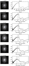Fig. 5. Impact of redshift effects on the bar analysis. The redshift effects include observational effects and galaxy (and bar) evolution. The symbols are the same as in Fig. 2, but we show simulated CEERS images at various redshifts and their results.

To illustrate the necessity of incorporating the galaxy evolution in generating simulated CEERS images, we created another set of simulated images considering only observational effects without any evolution. Figure 6 compares the two sets of simulated data using PGC049413 as an example. The left column shows the simulated images without any galaxy evolution models, and the right column shows the simulated images with the galaxy evolution models. As z increases, the bar structure gradually fades due to noise. At z = 3.0, the bar is still visible in the simulated CEERS image with evolution, but it appears to have completely faded into the background in images without evolution. The S/N of the images without evolution models (in intrinsic surface brightness) is significantly reduced due to the cosmological dimming effect on the observed galaxy surface brightness, which becomes fainter by 2.5log(1 + z)³ at high redshift (AB magnitude is used). However, the intrinsic surface brightness has been found to brighten with increasing redshift (e.g., Barden et al. 2005; Sobral et al. 2013), which is caused by a combination of luminosity evolution and size evolution (Yu et al. 2023). We calculated the S/N for these images and found that from z = 1.25, the S/N falls below 3 and is significantly lower than that for real CEERS images. At z = 3.0, the median value of S/N is only 0.54. The low S/N causes a large number of bars to be undetected. These noisy images are therefore inconsistent with the real CEERS galaxy images, which have a quite good S/N to resolve galaxy structures. This validates our procedure of generating simulated CEERS images by incorporating galaxy evolution models.

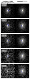Fig. 6. Simulated CEERS image with (on the right) and without (on the left) a galaxy evolution model using PGC049413 as an example, presented as the redshift increases. The blue ellipse marks the detected bar structure in the image if a bar is identified.

We caution that our bar evolution model may not be correct. Our input bar model assumed that the bar size related to the disk size remains unchanged across redshift. This ratio changes by a factor of ∼2 from z ∼ 3 to 0 in the simulations, however (Anderson et al. 2024). Future studies comparing fraction and size of bars observed in JWST images with simulated images may constrain the bar evolution model better.

4. Measurement robustness of bar structures

As illustrated in Sect. 3 through a representative example, the resolution limitation can significantly influence the identification and quantification of bars observed in the JWST CEERS field, while the effects of noise are negligible. These factors introduce considerable impact for galaxies at high redshift. In this section, we quantify these effects using the full sample of 448 galaxies.

4.1. Effect of resolution

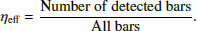
As the resolution decreases, bars may not be detected. For each set of simulated low-resolution images with the specific value of a_{bar,  true}/FWHM, we determined the method effectiveness of detecting bars (η_eff), defined as

$$\begin{array}{c}\hfill {\eta }_{\mathrm{eff}}=\frac{\mathrm{Number}\mathrm{of}\mathrm{detected}\mathrm{bars}}{\mathrm{All}\mathrm{bars}}.\end{array}$$(1)

We plot the η_eff as a function of resolution (n = a_{bar,  true}/FWHM) in Fig. 7, where the green diamonds, red circles, and gray squares denote the results for the F115W, F150W, and F200W filters, respectively. We calculated the error of each η_eff (and bar fraction) using the Wilson interval. With the a_{bar,  true}/FWHM decreasing from 10 to 1, the η_eff declines from 100% to nearly 0. However, the profile shape varies across different bands. For the F115W band, the η_eff stays at ∼100% until it reaches a_{bar,  true}/FWHM ≈ 3, after which it declines sharply. We calculate dthe a_{bar,  true}/FWHM corresponding to effectiveness of detecting bars of 50% through interpolation and obtained 2.47. For the F150W or F200W band, the η_eff does not decline sharply until it reaches a_{bar,  true}/FWHM ≈ 2. For the F150W and F200W band, the 50% effectiveness of detecting bars corresponds to a_{bar,  true}/FWHM = 1.71 and 1.65, respectively. Compared to the F150W and F200W bands, the F115W-band η_eff trend drops more sharply at higher a_{bar,  true}/FWHM. This is because, given the pixel size of 0.03 arcsec/pixel, the F115W PSF FWHM gives ∼1.2 pixels, which is significantly below the two-pixel threshold required for the Nyquist sampling. This inadequacy in sampling causes the F115W image to lose small-scale structure information, leading some short bars to become undetectable. Our results suggest that for images with a Nyquist-sampled PSF (e.g., JWST PSFs in the F200W, F277W, F356W, and F444W band), the critical bar size for detecting bars is 2 × FWHM, providing a quantitative justification for the empirical choice of a_{bar,  true} = 2 × FWHM as the bar size threshold for a bar detection by Erwin (2018). Erwin (2018) determined the factor of 2 because almost all the bars in the S⁴G sample are larger than 2 × FWHM.

Fig. 7. Effectiveness of the method of detecting bars, ηeff, as a function of resolution n = abar,  true/FWHM. The green diamonds, red circles, and gray squares represent the results based on the F115W, F150W, and F200W filters, respectively.

To understand how resolution can quantitatively impact the measured bar properties, we compared the properties ($a_{\text{obs}}^n$, ${ϵ}_{\mathrm{obs}}^n$, and ${\mathrm{PA}}_{\mathrm{obs}}^n$) derived from the low-resolution images with the intrinsic bar properties (a_{bar,  true}, ϵ_{bar,  true}, and PA_{bar,  true}) obtained from DESI images. 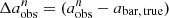We used the fractional difference $\mathrm{\Delta }{a}_{\mathrm{obs}}^n/a_{\mathrm{bar},\mathrm{true}}$, where $\mathrm{\Delta }{a}_{\mathrm{obs}}^n=(a_{\mathrm{obs}}^n-a_{\mathrm{bar},\mathrm{true}})$, to quantify the deviation in measured bar size as the resolution, n = a_{bar,  true}/FWHM, decreases. The number distributions of $\mathrm{\Delta }{a}_{\mathrm{obs}}^n/a_{\mathrm{bar},\mathrm{true}}$ at different n are shown in Fig. 8. The results for the F200W band are shown. In each panel, the n, the mean $\mathrm{\Delta }{a}_{\mathrm{obs}}^n$, denoted $\overline{\mathrm{\Delta }a/a}$, and the standard deviation of $\mathrm{\Delta }{a}_{\mathrm{obs}}^n$, denoted as σ_Δa/a, are presented. The vertical dashed line marks the location of $a_{\text{obs}}^n=a_{\text{bar},\hspace{0.17em}\text{true}}$. The overall distribution of $\mathrm{\Delta }{a}_{\text{obs}}^n/a_{\text{bar},\hspace{0.17em}\text{true}}$ is approximately symmetric. As n decreases from 10 to 2.49, the measured bar size tends to be increasingly underestimated, if slightly, from 1% to 6%. This underestimation is caused by PSF smoothing, as demonstrated in Fig. 2. However, as n decreases from 1.73 to 1, the measured bar size tends to be increasingly overestimated with lower resolution, from 2% to 19%. This can be explained by the fact that under relatively poor resolution conditions, various structures such as bars, spiral arms, and disks tend to become mixed. As a result, it becomes challenging to distinguish the bar distinctly, potentially leading to an overestimation of the measured bar size. The $\mathrm{\Delta }{a}_{\mathrm{obs}}^n/a_{\mathrm{bar},\mathrm{true}}$ as a function of n can be found in Fig. 9.

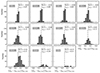Fig. 8. Distribution of the fractional difference $\mathrm{\Delta }{a}_{\text{obs}}^n/a_{\text{bar},\hspace{0.17em}\text{true}}$, where $\mathrm{\Delta }{a}_{\text{obs}}^n=(a_{\text{obs}}^n-a_{\text{bar},\hspace{0.17em}\text{true}})$, at various resolution levels n = abar,  true/FWHM. The abar,  true denotes the intrinsic value. We present the results for the F200W PSF. The averaged fractional difference ($\overline{\mathrm{\Delta }a/a}$) and standard deviation (σΔa/a) are indicated at the top of each panel. The vertical dashed black line in each panel marks $a_{\text{obs}}^n=a_{\text{bar},\hspace{0.17em}\text{true}}$.

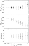Fig. 9. Change or fractional change between the measured parameters and their intrinsic values as a function of resolution n = abar,  true/FWHM. We present the results for the F200W filter.

In Fig. 10, we compare the intrinsic bar ellipcity ϵ_{bar,  true} with the measure bar ellipcity ${ϵ}_{\mathrm{obs}}^n$ that is obtained from images at each resolution level n = a_{bar,  true}/FWHM. The fractional difference is calculated as $\mathrm{\Delta }ϵ/ϵ=({ϵ}_{\mathrm{obs}}^n-{ϵ}_{\mathrm{bar},\mathrm{true}})/{ϵ}_{\mathrm{bar},\mathrm{true}}$. Their mean value ($\overline{\mathrm{\Delta }ϵ/ϵ}$) and standard deviation (σ_Δϵ/ϵ) is indicated in each panel. As the resolution decreases from n = 10 to 1, there is a clear trend that the data point distribution gradually shifts toward lower ${ϵ}_{\mathrm{obs}}^n$. This trend can be quantitatively observed by examining $\overline{\mathrm{\Delta }ϵ/ϵ}$, which decreases from −2% to −54%. Our results suggest that the PSF smoothing causes the measured bar ellipticity to be underestimated compared to its intrinsic value, and the underestimation becomes progressively more pronounced as the resolution decreases. Δϵ/ϵ as a function of n is shown in Fig. 9.

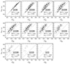Fig. 10. Comparison between ${ϵ}_{\mathrm{obs}}^n$ and ϵbar,  true at each resolution level n = abar,  true/FWHM. We present the results for the F200W filter. The fractional difference between ${ϵ}_{\mathrm{obs}}^n$ and ϵbar,  true is denoted $\mathrm{\Delta }ϵ/ϵ=({ϵ}_{\text{obs}}^n-{ϵ}_{\text{bar},\text{True}})/{ϵ}_{\text{bar},\text{True}}$. The mean value ($\overline{\mathrm{\Delta }ϵ/ϵ}$) and standard deviation (σΔϵ/ϵ) of the fractional difference are indicated in each panel. The one-to-one relation is displayed by the dashed line.

Regarding the robustness in measuring the orientation of bars, we compared PA${}_{\mathrm{obs}}^n$ with ${\mathrm{PA}}_{\mathrm{bar},\mathrm{true}}$ in Fig. 11. Their mean difference ($\overline{\mathrm{\Delta }\mathrm{PA}}$) and standard deviation (σ_ΔPA) are presented in each panel. Since the absolute value of PA does not necessarily reflect the physical significance, we did not normalize ΔPA by PA_{bar,  true}. Regardless of the resolution level, ${\text{PA}}_{\text{obs}}^n$ clearly remains consistently close to its intrinsic value. The absolute value of $\overline{\mathrm{\Delta }\mathrm{PA}}$ constantly stays at less than 1 degree. The ΔPA as a function of n is shown in Fig. 9. Our results indicate that the resolution affects the measurement of the orientation of the bar only little.

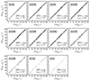Fig. 11. Comparison between ${\text{PA}}_{\text{obs}}^n$ and PAbar,  true at each resolution level n = abar,  true/FWHM. We present the results for the F200W filter. The difference between ${\text{PA}}_{\text{obs}}^n$ and PAbar,  true is denoted $\mathrm{\Delta }\text{PA}={\text{PA}}_{\text{obs}}^n-{\text{PA}}_{\text{bar},\hspace{0.17em}\text{true}}$. The mean difference ($\overline{\mathrm{\Delta }\mathrm{PA}}$) and standard deviation (σΔPA) are indicated in each panel. The one-to-one relation is displayed by the dashed line.

Figure 9 plots the previously discussed change or fractional change ($\mathrm{\Delta }{ϵ}_{\mathrm{obs}}^n/{ϵ}_{\mathrm{bar},\mathrm{true}}$, $\mathrm{\Delta }{a}_{\mathrm{obs}}^n/a_{\mathrm{bar},\mathrm{true}}$, and $\mathrm{\Delta }{\text{PA}}_{\text{obs}}^n$) between the parameters measured in low-resolution images generated using the F200W filter and their intrinsic values as a function of resolution (n = a_{bar,  true}/FWHM). These data, along with those obtained using F115W and F150W filters, are listed in Table 1. The dependence of $\mathrm{\Delta }{ϵ}_{\mathrm{obs}}^n/{ϵ}_{\mathrm{bar},\mathrm{true}}$, $\mathrm{\Delta }{a}_{\mathrm{obs}}^n/a_{\mathrm{bar},\mathrm{true}}$, and $\mathrm{\Delta }{\text{PA}}_{\text{obs}}^n$ on n for the F115W or F150W filter is quite similar to those for the F200W filter. However, as we showed in Fig. 7, η_eff for the F115W filter is lower than that for the F150W or F120W filters at a given n > 4 because the F115W PSF is not Nyquist-sampled at a pixel scale of 0.03 arcsec/pixel. We note that fewer than ten bars are identified at n = 1.44 and 1.2 for the F115W filter, at n = 1.2 for the F150W filter, and at n = 1 for the F200W filter, which might influence the statistical significance of the results at these n values.

4.2. Effect of noise

We investigated the influence of noise on the bar analysis by comparing the parameters ($a_{\mathrm{obs}}^{S/N}$, ${ϵ}_{\mathrm{obs}}^{S/N}$, and ${\mathrm{PA}}_{\mathrm{obs}}^{S/N}$), measured in the simulated low-S/N images and their noiseless values ($a_{\mathrm{obs}}^{n=4.3}$, ${ϵ}_{\mathrm{obs}}^{n=4.3}$, and ${\mathrm{PA}}_{\mathrm{obs}}^{n=4.3}$), measured in the noiseless low-resolution simulated images of n = 4.3. n was fixed to 4.3 to isolate the effects from noise. As these measurements are relatively robust against noise, we refrain from showing the plots, but list the results in Table 2. This table provides η_eff (Eq. (1)), and the mean value ($\overline{\mathrm{\Delta }{a}_{\mathrm{obs}}^{S/N}/a_{\mathrm{obs}}^{n=4.3}}$, $\overline{\mathrm{\Delta }{ϵ}_{\mathrm{obs}}^{S/N}/{ϵ}_{\mathrm{obs}}^{n=4.3}}$, and $\overline{\mathrm{\Delta }{\mathrm{PA}}_{\mathrm{obs}}^{S/N}}$) and standard deviation (${\sigma }_{\mathrm{\Delta }{a}_{\mathrm{obs}}^{S/N}/a_{\mathrm{obs}}^{n=4.3}}$, ${\sigma }_{\mathrm{\Delta }{ϵ}_{\mathrm{obs}}^{S/N}/{ϵ}_{\mathrm{obs}}^{n=4.3}}$, and ${\sigma }_{\mathrm{\Delta }{\text{PA}}_{\text{obs}}^{S/N}}$) of the change or fractional change in the measured parameters, defined in the same way as previously. Table 2 shows that when S/N ≥ 11.5, η_eff remains at 100%, suggesting that within this S/N range, all the barred galaxies can be detected. As the S/N falls below 11.5, a tiny fraction of barred galaxies can be missed. Nevertheless, even when the S/N reaches as low as 3, almost all the bars can be identified. Regardless of the S/N level, the deviation of the measured $a_{\mathrm{obs}}^{S/N}$, ${ϵ}_{\mathrm{obs}}^{S/N}$ and PA${}_{\mathrm{obs}}^{S/N}$ of the bars from their noiseless values is quite small, mostly ≤5% for a, ≤1% for ϵ, and ≤0.5 degree for PA, although the scatter increases slightly with lower S/N. This analysis was also performed for the noiseless simulated images of other values of a_{bar,  true}/FWHM, and the results are almost identical to those in Table 2. Our results suggest that for the typical S/N range in CEERS for galaxies with a redshift of z ≤ 3 and a stellar mass of M_⋆ ≥ 10^9.75 M_⊙, the detection and quantification of bars is not significantly adversely affected by the noise.

In practical applications, it is more straightforward to calculate the effective surface brightness (μ_e), which has a similar ability to characterize the clarity of an extended structure to the S/N for a given background noise. To facilitate the use of our results, we computed the mean value of μ_e ($\overline{{\mu }_e}$) for our simulated images at each S/N level and list them in Table 2. As our simulated images were generated to match the typical noise conditions in the CEERS field, the values of $\overline{{\mu }_e}$ only work robustly in the CEERS field. These $\overline{{\mu }_e}$, corresponding to a given S/N, should be fainter in a survey deeper than CEERS, but brighter in a shallower survey.

4.3. Bar identification and measurement in simulated CEERS images

In this section, we explore how the identification and quantification of bars at high redshifts is influenced by the combination of observational and evolution effects using the simulated CEERS images with galaxy evolution models. The dependence of the method effectiveness of detecting bars (η_eff; on the left y-axis) and the observed bar fraction (f_{bar,  obs}; on the right y-axis) on redshift z is shown by the gray diamonds in Fig. 12. The error bars associated with the data points are the uncertainty of f_{bar,  obs}. The f_{bar,  obs} is defined as the ratio of the number of bars identified at each redshift to the total number of disk galaxies,

$$\begin{array}{c}\hfill f_{\mathrm{bar},\mathrm{obs}}=\frac{\mathrm{Number}\mathrm{of}\mathrm{detected}\mathrm{bars}}{\mathrm{Number}\mathrm{of}\mathrm{disks}}.\end{array}$$(2)

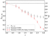Fig. 12. Dependence of the fraction of bars (fbar,  obs) and effectiveness of detecting bars (ηeff), measured from the simulated CEERS images as a function of redshift (z). The gray diamonds represent the results obtained from the simulated data with the galaxy evolution model, and the pink stars represent those from the data without a model. The error bars denote the uncertainty of fbar,  obs. For the simulated CEERS images, the F115W, F150W, and F200W filters are used for redshift range z = 0.75–1.0, 1.25–1.75, and 2.0–3.0, respectively. The horizontal dashed line represents the fbar,  true of 68% of our sample.

As the redshift increases from 0 to 3, η_eff gradually decreases. It declines from 100% to approximately 55%, suggesting that increasingly more bars are missing at higher redshift due to the impact of observational effects. Approximately half of the bars can remain undetected at z = 3. f_{bar,  obs} decreases from 68% to 37.5%, suggesting that the bar fraction observed at the JWST F200W band can be underestimated by 30% at z = 3 compared to the local Universe. The η_eff-z and f_{bar,  obs}-z relations are not smooth, but present two sudden declines at z = 1.0 and z = 1.75, which stem from the changes of the filters. From z = 1.0 to z = 1.25, for better tracing the rest-frame optical light, the F115W is changed to F150W, the image PSFs broadens, causing the images to become blurrier and thus reducing the bar detection capability. When the F150W filter is changed to F200W at z = 2.0, the same principle applies. The trend of decreasing apparent f_{bar,  obs} with increasing z is consistent with Erwin (2018), who used S⁴G images to simulate the resolution of high-redshift HST images and generated a decreasing trend of the bar fraction toward higher redshift by applying a cut in the bar size to select barred galaxies.

For comparison, we show the results for the simulated images without involving galaxy evolution as pink stars in Fig. 12. The measured f_{bar,  obs} at z ≤ 1.25 is almost identical to the results from the simulated CEERS image with galaxy evolution. However, as the redshift increases, the f_{bar,  obs} decreases significantly, reaching 11% at z = 3.0. This decrease occurs because the S/N is too low due to the cosmological dimming effect, as discussed in Sect. 3.

In Fig. 13, we plot the fractional difference ($\mathrm{\Delta }{a}_{\text{obs}}^z/a_{\text{bar},\hspace{0.17em}\text{true}}$, $\mathrm{\Delta }{ϵ}_{\text{obs}}^z/{ϵ}_{\text{bar},\hspace{0.17em}\text{true}}$) or absolute difference ($\mathrm{\Delta }{\text{PA}}_{\text{obs}}^z$) between the three parameters measured from the simulated CEERS images at each redshift and their intrinsic values. As shown in the top row, the $\mathrm{\Delta }{a}_{\mathrm{obs}}^z/a_{\mathrm{bar},\mathrm{true}}$ at each redshift is slightly lower than zero on average, suggesting that the bar size measurements at higher redshift are relatively robust, with an underestimation of only a few percent (≤4%). The relation between $\mathrm{\Delta }{a}_{\mathrm{obs}}^z/a_{\mathrm{bar},\mathrm{true}}$ and z does not reveal the systematic overestimation in measured bar size when the resolution is very low, as might be expected from Fig. 9. This is because most short bars with size a_{bar,  true} ≲ 2 × FWHM have been missed (Fig. 7) in the process of bar identification for the simulated CEERS images. Specifically, at z = 3, 90% of the identified bars have a size a_{bar,  true} > 2 × FWHM, which leads to a minor underestimation of the measured bar size according to Fig. 9. The relation between $\mathrm{\Delta }{ϵ}_{\mathrm{obs}}^z/{ϵ}_{\mathrm{bar},\mathrm{true}}$ and z shows that the measured bar ellipticities are increasingly underestimated at redshift increasing from z = 0.75 to z = 2.0 on average, but the underestimation becomes approximately constant beyond z = 2.0. As galaxies become smaller in their angle at high redshifts, the $\mathrm{\Delta }{ϵ}_{\mathrm{obs}}^z/{ϵ}_{\mathrm{bar},\mathrm{true}}$ might be thought to decrease strictly monotonically with higher z according to Fig. 9, but this conjecture is not true. The decline in $\mathrm{\Delta }{ϵ}_{\mathrm{obs}}^z/{ϵ}_{\mathrm{bar},\mathrm{true}}$ from z = 0.75 to z = 2 is indeed due to the significant reduction in the angular size of galaxies, in which effects from longer distance and size evolution of the disks are considered. However, at higher redshift, more and more bars become too small in their angular size to be detected, so that the contribution of the severe underestimation in ϵ caused by short bars in the calculation of mean value is significantly reduced, leading to an approximately constant average $\mathrm{\Delta }{ϵ}_{\mathrm{obs}}^z/{ϵ}_{\mathrm{bar},\mathrm{true}}$ between z = 2 and z = 3. As expected, the measurement of PA is quite robust without any obvious systematic biases.

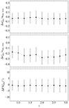Fig. 13. Fractional difference ($\mathrm{\Delta }{a}_{\text{obs}}^z/a_{\text{bar},\hspace{0.17em}\text{true}}$ and $\mathrm{\Delta }{ϵ}_{\text{obs}}^z/{ϵ}_{\text{bar},\hspace{0.17em}\text{true}}$ or absolute difference ($\mathrm{\Delta }{\text{PA}}_{\text{obs}}^z$) between the parameters measured from the simulated CEERS images and their intrinsic values plotted against redshift (z). The error bar represents the standard deviation of the results at each redshift.

4.4. Correction of the measurement biases

While the PA measurement remains unbiased, the measurements of a and ϵ are biased toward lower values at high redshift, with resolution effects being the primary cause. With the fractional differences between the measurements from the low-resolution images and their intrinsic values listed in Table 1, we can effectively remove the biases introduced by resolution. The bias-corrected bar size, denoted $a_{\text{cor}}^z$, can be obtained through

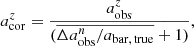$$\begin{array}{c}\hfill a_{\mathrm{cor}}^z=\frac{a_{\mathrm{obs}}^z}{(\overline{\mathrm{\Delta }{a}_{\mathrm{obs}}^n/a_{\mathrm{bar},\mathrm{true}}}+1)},\end{array}$$(3)

where n is approximated as $a_{\mathrm{obs}}^z/FWHM$, and the value of $\overline{\mathrm{\Delta }{a}_{\mathrm{obs}}^n/a_{\mathrm{bar},\mathrm{true}}}$ is obtained via interpolation based on the data in Table 1. The same method can be applied to obtain the bias-corrected bar ellipticity, denoted ${ϵ}_{\text{cor}}^z$,

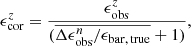$$\begin{array}{c}\hfill {ϵ}_{\mathrm{cor}}^z=\frac{{ϵ}_{\mathrm{obs}}^z}{(\overline{\mathrm{\Delta }{ϵ}_{\mathrm{obs}}^n/{ϵ}_{\mathrm{bar},\mathrm{true}}}+1)},\end{array}$$(4)

where the value of $\overline{\mathrm{\Delta }{ϵ}_{\mathrm{obs}}^n/{ϵ}_{\mathrm{bar},\mathrm{true}}}$ is obtained through interpolation. Figure 14 plots the fractional difference ($\mathrm{\Delta }{a}_{\text{cor}}^z/a_{\text{bar},\hspace{0.17em}\text{true}}$) between $a_{\text{cor}}^z$ and its intrinsic value a_{bar,  true} in the top panel and the fractional difference ($\mathrm{\Delta }{ϵ}_{\text{cor}}^z/{ϵ}_{\text{bar},\hspace{0.17em}\text{true}}$) between ${ϵ}_{\text{cor}}^z$ and its intrinsic value ϵ_{bar,  true} in the bottom panel. After making corrections, the values of $a_{\text{cor}}^z$ and ${ϵ}_{\text{cor}}^z$ underestimate a_{bar,  true} and ϵ_{bar,  true} by less than 1% on average. The residuals are negligibly small, indicating that our correction functions are effective.

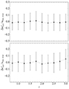Fig. 14. Fractional difference ($\mathrm{\Delta }{a}_{\text{cor}}^z/a_{\text{bar},\hspace{0.17em}\text{true}}$ and $\mathrm{\Delta }{ϵ}_{\text{cor}}^z/{ϵ}_{\text{bar},\hspace{0.17em}\text{true}}$) between bias-corrected parameters measured from the simulated CEERS images and their intrinsic values plotted against redshift (z). The error bar represents the standard deviation of the results at a given redshift.

5. Implication

Determining the bar fraction at high redshift is crucial for understanding the nature of bars, but it is challenging because the band shifts and/or the image degrades (Sheth et al. 2008). An early HST-based study of the bar fraction evolution reported a significant decrease beyond z ∼ 0.5 (Abraham et al. 1999). Then Sheth et al. (2003) found that the fraction of strong bars at z > 0.7 (4/95) is higher than the fraction observed at z < 0.7 (1/44). These fractions are likely lower limits, primarily due to resolution effects and the small-number statistic. With improved resolution images obtained from the HST Advanced Camera for Surveys (ACS), two subsequent studies of Elmegreen et al. (2004) and Jogee et al. (2004) reported a relatively consistent fraction up to redshift z ∼ 1. Nevertheless, their samples are still of a modest size. With a statistically large sample of more than 2000 galaxies defined from the Cosmic Evolution Survey (COSMOS; Scoville et al. 2007, Sheth et al. 2008) showed that the bar fraction declines from ∼65% in the local Universe to ∼20% at z ≈ 0.84. Although the overall bar fractions calculated based on the Galaxy Zoo were underestimated (Erwin 2018), studies based on it have consistently identified a trend that declines from ∼22% at z = 0.4 to ∼11% at z = 1.0 (Melvin et al. 2014).

Previous studies have consistently raised concerns about the possibility that short bars at higher redshift might be missed due to resolution limitations. Lacking rigorous quantitative justification, Sheth et al. (2003) proposed a bar size threshold of 2.5 times the PSF FWHM for a bar detection. Concluding from experiments on artificial galaxies, Aguerri et al. (2009) proposed the same the threshold. Erwin (2018) suggested a lower threshold of twice the PSF FWHM. In Fig. 7, we demonstrate that for images with a Nyquist-sampled PSF, the effectiveness of detecting bars η_eff remains at ∼100% when a_{bar,  true}/FWHM is above 2. When a_{bar,  true}/FWHM is below 2, the η_eff declines sharply. We selected the bars in the simulated CEERS images using the criterion a_{bar,  true} > F200WFWHM, calculated the f_{bar,  obs}, and plotted them as pink square in Fig. 15. These f_{bar,  obs} are fully consistent with the F200W-band f_{bar,  obs} derived from the ellipse-fitting method, which are represented as gray diamonds in the plot. This suggests that using a_{bar,  true} = 2 × FWHM as the bar detection threshold provides a better fit to the results obtained through the ellipse-fitting method. Using the factor of 2.5 would underestimate the bar-detection efficiency of the ellipse-fitting method. Nevertheless, if the PSFs are not Nyquist-sampled, the effectiveness of detecting bars starts to decline at higher a_{bar,  true}/FWHM, suggesting a higher bar size threshold. The concern that bars might be missed due to resolution effects is further amplified by the growth of the bar size over cosmic time, as indicated by simulation studies (e.g., Debattista & Sellwood 2000; Martinez-Valpuesta et al. 2006; Algorry et al. 2017; Rosas-Guevara et al. 2022).

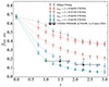Fig. 15. Measured bar fraction (fbar, obs) obtained from simulated CEERS images as a function of redshift (z). The gray diamonds represent the fbar, obs obtained using the ellipse-fitting method for simulated CEERS images. The other symbols mark the results obtained by adopting the criterion of abar, true > 2 × FWHM for a bar detection for specific JWST NIRcam filters. The pink rectangles, brown inverted triangles, blue dots, and green stars represent the fbar, obs for F200W, F277W, F356W, and F444W filter, respectively. The black triangles correspond to the observed F444W-band bar fraction measured by Le Conte et al. (2024).

Studies of bars based on cosmological simulations also highlight the potential impact arising from resolution effects. By studying TNG100 galaxies, Zhao et al. (2020) revealed a roughly constant bar fraction of ∼60% at 0 < z < 1 when selecting galaxies with a mass cut of M_⋆ ≥ 10^10.6 M_⊙. However, considering the resolution limitations observed in HST images, where bars shorter than 2 kpc can be missed at z ∼ 1, they focused on bars longer than 2.2 kpc and consequently detected a decreasing trend of the bar fraction at higher redshift. Moreover, Rosas-Guevara et al. (2022) used the data from TNG50 to study spiral galaxies with M_⋆ ≥ 10¹⁰ M_⊙, showing that the derived bar fraction increases from 28% at z = 4, and reaches a peak of 48% at z = 1 and then drops to 30% at z = 0. Considering the 2 × FWHM detection limit, they implemented an angular resolution limit equivalent to twice the HST F814W PSF FWHM. As a result, the bar fraction exhibited a decrease with increasing redshift at z > 0.5, which reconciles the differences between their results and observations to some extent.

With the advent of JWST, obtaining deep high-resolution NIR images has become possible, enabling us to explore the structures in high-redshift galaxies in detail. Recently, Guo et al. (2023) analyzed rest-frame NIR galaxy structures using F444W images from JWST CEERS and reported the detection of six strongly barred galaxies at 1 < z < 3.

Costantin et al. (2023) remarkably reported a barred galaxy at z ≃ 3 from CEERS, making it the most distant barred galaxy ever detected. This discovery suggests that dynamically cold disk galaxies could have already been in place at z = 4 − 5. Our findings, derived from simulated CEERS data, can serve as a comparison sample for studies of the high-redshift bar fraction based on JWST. The gray diamonds in Figure 15 plot the observed f_{bar,  obs} from the simulated CEERS images in the F115W band for z = 0.75–1.0, in the F150W band for z = 1.25–1.75, and in the F200W band for z = 2.0–3.0. We restate that the CEERS image simulation procedure incorporates the changes in angular size due to both distance and the intrinsic evolution of disk size. As a result, bars in the simulated CEERS images appear to be shorter in physical size at higher redshift, directly following the disk size evolution described by van der Wel et al. (2014). Specifically, at redshifts z = 1, z = 2, and z = 3, bars are approximately 63%, 48%, and 40% of the size of their local counterparts. In contrast, the ratio of the bar size to the disk size remains unchanged, and the true bar fraction is fixed to 68%, the value measured in DESI images (Sect. 2). To present the results based on other long-wavelength NIRcam filters (F277W, F356W, and F444W), we estimated the measured f_{bar,  obs} using the current simulated dataset by adopting the criterion of a_{bar,  true} > 2 × FWHM for the bar detection, as proposed by Erwin (2018). First, we applied a_{bar,  true} > 2 × F200WFWHM to detect bars, calculated f_{bar,  obs} observed in the F200W band, and plotted them as pink squares in Fig. 15. They agree well with the results at redshift 2 ≤ z ≤ 3 obtained from the ellipse-fitting method, demonstrating the effectiveness of the a_{bar,  true} > 2 × F200WFWHM criterion. Subsequently, using a_{bar,  true} > 2 × F277WFWHM, we calculated the F277W-band f_{bar,  obs} observed in the simulated CEERS images, and plotted them as green stars. The observed f_{bar,  obs} in the F277W band is lower than its F200W-band counterpart because the F277W PSF FWHM is larger than the F200W PSF FWHM. The same calculations were applied to the F356W and F444W bands. We summarize the measured values of f_{bar,  obs} as a function of redshifts for the four NIRcam bands in Table 3.

We note that the F444W-band f_{bar,  obs} decreases significantly from 68% at z ≈ 0 to 13% at z = 1.5, and further to 6% at z = 3.0. We plot the F444W-band bar fraction observed in JWST CEERS and the Public Release Imaging for Extragalactic Research (PRIMER; Dunlop et al. 2021) measured by Le Conte et al. (2024) as black triangles in Fig. 15. The F444W-band f_{bar,  obs} from the simulated CEERS images is consistent within 1 σ uncertainty with those obtained from JWST F444W-band observations reported in Le Conte et al. (2024), despite the potential difference in the sample properties. Therefore, by accounting for resolution effects and bar size evolution, we have successfully reproduced the bar fraction observed by JWST in the F444W band without the evolution of the intrinsic bar fraction. Our findings are consistent with Erwin (2018), who similarly factored in resolution effects and assumed bar sizes to be half their actual values at high redshifts. Using S⁴G images for simulated observations, they reproduced the relation between the observed bar fraction and stellar mass at redshifts up to 0.84, as reported by Sheth et al. (2008). Our results imply that by positing the presence of all local bars as early as z ∼ 3, the combination of resolution effects and bar size growth can largely accounted for the apparent redshift evolution in the observed bar fraction found by Le Conte et al. (2024). Any intrinsic evolution in the bar fraction, if it exists, might be artificially exaggerated by these factors. To truly grasp the evolution of the intrinsic bar fraction, it is imperative to disentangle it from resolution effects and bar size evolution.

6. Conclusions

Quantifying the evolution of bar fraction and bar properties is essential for understanding the evolutionary history of disk galaxies. During the HST era, a series of studies have explored this subject extensively (e.g., Elmegreen et al. 2004; Jogee et al. 2004; Sheth et al. 2008; Pérez et al. 2012; Melvin et al. 2014; Kim et al. 2021). However, these results are potentially affected by limitations of image quality. With the superior high-resolution and deep NIR imaging available from JWST, bars in galaxies at high redshift can be studied today in far more detail, and some bars at z > 2 have been successfully detected (Guo et al. 2023; Le Conte et al. 2024). The difficulties caused by limited observations are still unavoidable, making it challenging to fully embrace the intrinsic results. To assess our ability to analyze bars in high-redshift galaxies observed by JWST, we used a sample of 448 nearby face-on spiral galaxies, a subset of the sample conducted by Yu et al. (2023), to simulate images under various observational conditions consistent with the JWST CEERS field, identify bars, and quantify bar properties, and then compared the results before and after the simulation to determine the systematic biases arising from the resolution, the noise, or a combination of the two. The intrinsic bar size is denoted as a_{bar,  true}. The ratio a_{bar,  true}/FWHM was used to gauge the detectability of bars. Our main findings are summarized below.

1. The identification and quantification of bars are hardly affected by noise when the S/N is greater than 3, an observational condition met by CEERS galaxies with M_⋆ ≥ 10^9.75 M_⊙ at z < 3.

2. For the F200W PSF, which is Nyquist-sampled, the effectiveness of detecting bars remains at ∼1 when a_{bar,  true}/FWHM is above a critical value of 2; when a_{bar,  true}/FWHM is below 2, the effectiveness drops sharply. The fractions of bars determined through the ellipse-fitting method agrees well with that derived using the criterion a_{bar,  true} > 2 × FWHM, the bar size threshold suggested by Erwin (2018) for a bar detection. Nevertheless, when the PSF is sub-Nyquist-sampled, the critical a_{bar,  true}/FWHM increases. For instance, for the F115W PSF at a pixel scale of 0.03 arcsec/pixel, this critical value is ∼3.

3. By assuming all local bars were already in place at high redshift, we showed that a combination of resolution effects and bar size growth can explain the apparent evolution of bar fraction obtained from JWST observations reported by Le Conte et al. (2024). This implies that the reported bar fraction has been significantly underestimated. The true bar fraction evolution, if it exists, could be shallower than detected. Our results underscore the importance of disentangling the true bar fraction evolution from resolution effects and bar size growth.

4. The measured bar size and bar ellipticity are typically underestimated, with the extent depending on a_{bar,  true}/FWHM. In contrast, the measurement of the bar position angle remains unaffected by resolution. To remove these resolution effects, we developed correction functions. When applied to the bar properties measured from the simulated CEERS images of high-redshift galaxies, these corrections yield bias-corrected values that closely match their intrinsic values.

Acknowledgments

This work was supported by the National Science Foundation of China (11721303, 11890692, 11991052, 12011540375, 12133008, 12221003, 12233001), the National Key R&D Program of China (2017YFA0402600, 2022YFF0503401), and the China Manned Space Project (CMS-CSST-2021-A04, CMS-CSST-2021-A06). We thank the referee for his insightful and constructive feedback, which significantly enhanced the quality and clarity of this letter. SYY acknowledges the support by the Alexander von Humboldt Foundation. Kavli IPMU is supported by World Premier International Research Center Initiative (WPI), MEXT, Japan.

References

All Tables

All Figures

	Fig. 1. Basic properties of the barred galaxies in our sample. The left panel illustrates the distribution of the bar ellipticity (ϵbar,  true), and the right panel shows the projected bar size as semi-major axis (abar,  true) vs. stellar mass (M⋆).
In the text

Fig. 2. Impact of the decreasing resolution on the bar analysis, using PGC049413 as an example. On the left are the galaxy images, and their respective derived ϵ profiles are shown at the right. At the top of each image, the ratio of abar,  true to the FWHM is indicated. The first row shows the results from DESI, succeeded by the results from low-resolution F200W images in the rows below. The DESI ϵ profiles are plotted with dashed gray curves in the right panels. The intrinsic bar position is denoted as the vertical dashed gray line. When a bar is successfully identified, it is marked in the image by an ellipse and indicated in the profile by a vertical solid line.

In the text

	Fig. 3. Impact of the decreasing resolution on the bar analysis, using NGC0514 as another example. The details are the same as in Fig. 2.
In the text

	Fig. 4. Impact of noise on the bar analysis. The symbols are the same as in Fig. 2. The top row now displays the noiseless simulated image of abar,  true/FWHM = 4.3 and its profile, and the subsequent rows show the simulated low-S/N images and their profiles.
In the text

	Fig. 5. Impact of redshift effects on the bar analysis. The redshift effects include observational effects and galaxy (and bar) evolution. The symbols are the same as in Fig. 2, but we show simulated CEERS images at various redshifts and their results.
In the text

	Fig. 6. Simulated CEERS image with (on the right) and without (on the left) a galaxy evolution model using PGC049413 as an example, presented as the redshift increases. The blue ellipse marks the detected bar structure in the image if a bar is identified.
In the text

	Fig. 7. Effectiveness of the method of detecting bars, ηeff, as a function of resolution n = abar,  true/FWHM. The green diamonds, red circles, and gray squares represent the results based on the F115W, F150W, and F200W filters, respectively.
In the text

Fig. 8. Distribution of the fractional difference $\mathrm{\Delta }{a}_{\text{obs}}^n/a_{\text{bar},\hspace{0.17em}\text{true}}$, where $\mathrm{\Delta }{a}_{\text{obs}}^n=(a_{\text{obs}}^n-a_{\text{bar},\hspace{0.17em}\text{true}})$, at various resolution levels n = abar,  true/FWHM. The abar,  true denotes the intrinsic value. We present the results for the F200W PSF. The averaged fractional difference ($\overline{\mathrm{\Delta }a/a}$) and standard deviation (σΔa/a) are indicated at the top of each panel. The vertical dashed black line in each panel marks $a_{\text{obs}}^n=a_{\text{bar},\hspace{0.17em}\text{true}}$.

In the text

	Fig. 9. Change or fractional change between the measured parameters and their intrinsic values as a function of resolution n = abar,  true/FWHM. We present the results for the F200W filter.
In the text

Fig. 10. Comparison between ${ϵ}_{\mathrm{obs}}^n$ and ϵbar,  true at each resolution level n = abar,  true/FWHM. We present the results for the F200W filter. The fractional difference between ${ϵ}_{\mathrm{obs}}^n$ and ϵbar,  true is denoted $\mathrm{\Delta }ϵ/ϵ=({ϵ}_{\text{obs}}^n-{ϵ}_{\text{bar},\text{True}})/{ϵ}_{\text{bar},\text{True}}$. The mean value ($\overline{\mathrm{\Delta }ϵ/ϵ}$) and standard deviation (σΔϵ/ϵ) of the fractional difference are indicated in each panel. The one-to-one relation is displayed by the dashed line.

In the text

Fig. 11. Comparison between ${\text{PA}}_{\text{obs}}^n$ and PAbar,  true at each resolution level n = abar,  true/FWHM. We present the results for the F200W filter. The difference between ${\text{PA}}_{\text{obs}}^n$ and PAbar,  true is denoted $\mathrm{\Delta }\text{PA}={\text{PA}}_{\text{obs}}^n-{\text{PA}}_{\text{bar},\hspace{0.17em}\text{true}}$. The mean difference ($\overline{\mathrm{\Delta }\mathrm{PA}}$) and standard deviation (σΔPA) are indicated in each panel. The one-to-one relation is displayed by the dashed line.

In the text

Fig. 12. Dependence of the fraction of bars (fbar,  obs) and effectiveness of detecting bars (ηeff), measured from the simulated CEERS images as a function of redshift (z). The gray diamonds represent the results obtained from the simulated data with the galaxy evolution model, and the pink stars represent those from the data without a model. The error bars denote the uncertainty of fbar,  obs. For the simulated CEERS images, the F115W, F150W, and F200W filters are used for redshift range z = 0.75–1.0, 1.25–1.75, and 2.0–3.0, respectively. The horizontal dashed line represents the fbar,  true of 68% of our sample.

In the text

Fig. 13. Fractional difference ($\mathrm{\Delta }{a}_{\text{obs}}^z/a_{\text{bar},\hspace{0.17em}\text{true}}$ and $\mathrm{\Delta }{ϵ}_{\text{obs}}^z/{ϵ}_{\text{bar},\hspace{0.17em}\text{true}}$ or absolute difference ($\mathrm{\Delta }{\text{PA}}_{\text{obs}}^z$) between the parameters measured from the simulated CEERS images and their intrinsic values plotted against redshift (z). The error bar represents the standard deviation of the results at each redshift.

In the text

Fig. 14. Fractional difference ($\mathrm{\Delta }{a}_{\text{cor}}^z/a_{\text{bar},\hspace{0.17em}\text{true}}$ and $\mathrm{\Delta }{ϵ}_{\text{cor}}^z/{ϵ}_{\text{bar},\hspace{0.17em}\text{true}}$) between bias-corrected parameters measured from the simulated CEERS images and their intrinsic values plotted against redshift (z). The error bar represents the standard deviation of the results at a given redshift.

In the text

Fig. 15. Measured bar fraction (fbar, obs) obtained from simulated CEERS images as a function of redshift (z). The gray diamonds represent the fbar, obs obtained using the ellipse-fitting method for simulated CEERS images. The other symbols mark the results obtained by adopting the criterion of abar, true > 2 × FWHM for a bar detection for specific JWST NIRcam filters. The pink rectangles, brown inverted triangles, blue dots, and green stars represent the fbar, obs for F200W, F277W, F356W, and F444W filter, respectively. The black triangles correspond to the observed F444W-band bar fraction measured by Le Conte et al. (2024).

In the text

References

- Abraham, R. G., Tanvir, N. R., Santiago, B. X., et al. 1996, MNRAS, 279, L47 [Google Scholar]
- Abraham, R. G., Merrifield, M. R., Ellis, R. S., Tanvir, N. R., & Brinchmann, J. 1999, MNRAS, 308, 569 [NASA ADS] [CrossRef] [Google Scholar]
- Aguerri, J. A. L., Beckman, J. E., & Prieto, M. 1998, AJ, 116, 2136 [NASA ADS] [CrossRef] [Google Scholar]
- Aguerri, J. A. L., Méndez-Abreu, J., & Corsini, E. M. 2009, A&A, 495, 491 [NASA ADS] [CrossRef] [EDP Sciences] [Google Scholar]
- Algorry, D. G., Navarro, J. F., Abadi, M. G., et al. 2017, MNRAS, 469, 1054 [Google Scholar]
- Anderson, S. R., Gough-Kelly, S., Debattista, V. P., et al. 2024, MNRAS, 527, 2919 [Google Scholar]
- Athanassoula, E. 1992, MNRAS, 259, 345 [Google Scholar]
- Athanassoula, E. 2002, ApJ, 569, L83 [NASA ADS] [CrossRef] [Google Scholar]
- Athanassoula, E. 2013, in Secular Evolution of Galaxies, eds. J. Falcón-Barroso, & J. H. Knapen, 305 [CrossRef] [Google Scholar]
- Athanassoula, E., & Misiriotis, A. 2002, MNRAS, 330, 35 [Google Scholar]
- Athanassoula, E., Lambert, J. C., & Dehnen, W. 2005, MNRAS, 363, 496 [Google Scholar]
- Bagley, M. B., Finkelstein, S. L., Koekemoer, A. M., et al. 2023, ApJ, 946, L12 [NASA ADS] [CrossRef] [Google Scholar]
- Barazza, F. D., Jogee, S., & Marinova, I. 2008, ApJ, 675, 1194 [Google Scholar]
- Barbary, K. 2016, J. Open Source Software, 1, 58 [NASA ADS] [CrossRef] [Google Scholar]
- Barden, M., Rix, H.-W., Somerville, R. S., et al. 2005, ApJ, 635, 959 [NASA ADS] [CrossRef] [Google Scholar]
- Bertin, E., & Arnouts, S. 1996, A&AS, 117, 393 [NASA ADS] [CrossRef] [EDP Sciences] [Google Scholar]
- Buta, R., Laurikainen, E., Salo, H., & Knapen, J. H. 2010, ApJ, 721, 259 [NASA ADS] [CrossRef] [Google Scholar]
- Buta, R. J., Sheth, K., Athanassoula, E., et al. 2015, ApJS, 217, 32 [Google Scholar]
- Cameron, E., Carollo, C. M., Oesch, P., et al. 2010, MNRAS, 409, 346 [NASA ADS] [CrossRef] [Google Scholar]
- Cavanagh, M. K., Bekki, K., & Groves, B. A. 2023, MNRAS, 520, 5885 [CrossRef] [Google Scholar]
- Conselice, C. J., Rajgor, S., & Myers, R. 2008, MNRAS, 386, 909 [CrossRef] [Google Scholar]
- Costantin, L., Pérez-González, P. G., Guo, Y., et al. 2023, Nature, 623, 499 [NASA ADS] [CrossRef] [Google Scholar]
- Debattista, V. P., & Sellwood, J. A. 2000, ApJ, 543, 704 [Google Scholar]
- Desai, V., Dalcanton, J. J., Aragón-Salamanca, A., et al. 2007, ApJ, 660, 1151 [NASA ADS] [CrossRef] [Google Scholar]
- de Vaucouleurs, G., de Vaucouleurs, A., Corwin, Herold G. J., et al. 1991, Third Reference Catalogue of Bright Galaxies (New York, NY: Springer) [Google Scholar]
- Dey, A., Schlegel, D. J., Lang, D., et al. 2019, AJ, 157, 168 [Google Scholar]
- Díaz-García, S., Salo, H., Laurikainen, E., & Herrera-Endoqui, M. 2016, A&A, 587, A160 [NASA ADS] [CrossRef] [EDP Sciences] [Google Scholar]
- Dunlop, J. S., Abraham, R. G., Ashby, M. L. N., et al. 2021, PRIMER: Public Release IMaging for Extragalactic Research, JWST Proposal. Cycle 1, ID. #1837 [Google Scholar]
- Ellison, S. L., Nair, P., Patton, D. R., et al. 2011, MNRAS, 416, 2182 [NASA ADS] [CrossRef] [Google Scholar]
- Elmegreen, B. G., & Elmegreen, D. M. 1985, ApJ, 288, 438 [Google Scholar]
- Elmegreen, B. G., Elmegreen, D. M., & Hirst, A. C. 2004, ApJ, 612, 191 [NASA ADS] [CrossRef] [Google Scholar]
- Elmegreen, B. G., Elmegreen, D. M., Knapen, J. H., et al. 2007, ApJ, 670, L97 [NASA ADS] [CrossRef] [Google Scholar]
- Erwin, P. 2005, MNRAS, 364, 283 [Google Scholar]
- Erwin, P. 2018, MNRAS, 474, 5372 [Google Scholar]
- Erwin, P. 2019, MNRAS, 489, 3553 [NASA ADS] [CrossRef] [Google Scholar]
- Erwin, P., & Debattista, V. P. 2013, MNRAS, 431, 3060 [Google Scholar]
- Erwin, P., & Sparke, L. S. 2003, ApJS, 146, 299 [NASA ADS] [CrossRef] [Google Scholar]
- Ferreira, L., Adams, N., Conselice, C. J., et al. 2022, ApJ, 938, L2 [NASA ADS] [CrossRef] [Google Scholar]
- Ferreira, L., Conselice, C. J., Sazonova, E., et al. 2023, ApJ, 955, 94 [NASA ADS] [CrossRef] [Google Scholar]
- Finkelstein, S. L., Bagley, M. B., Haro, P. A., et al. 2022, ApJ, 940, L55 [NASA ADS] [CrossRef] [Google Scholar]
- Gadotti, D. A. 2009, MNRAS, 393, 1531 [Google Scholar]
- Gadotti, D. A. 2011, MNRAS, 415, 3308 [Google Scholar]
- Gadotti, D. A., Bittner, A., Falcón-Barroso, J., et al. 2020, A&A, 643, A14 [NASA ADS] [CrossRef] [EDP Sciences] [Google Scholar]
- Gavazzi, G., Consolandi, G., Dotti, M., et al. 2015, A&A, 580, A116 [NASA ADS] [CrossRef] [EDP Sciences] [Google Scholar]
- Guo, Y., Jogee, S., Finkelstein, S. L., et al. 2023, ApJ, 945, L10 [NASA ADS] [CrossRef] [Google Scholar]
- Herrera-Endoqui, M., Díaz-García, S., Laurikainen, E., & Salo, H. 2015, A&A, 582, A86 [NASA ADS] [CrossRef] [EDP Sciences] [Google Scholar]
- Ho, L. C., Li, Z.-Y., Barth, A. J., Seigar, M. S., & Peng, C. Y. 2011, ApJS, 197, 21 [Google Scholar]
- Jacobs, C., Glazebrook, K., Calabrò, A., et al. 2023, ApJ, 948, L13 [NASA ADS] [CrossRef] [Google Scholar]
- Jogee, S., Barazza, F. D., Rix, H.-W., et al. 2004, ApJ, 615, L105 [NASA ADS] [CrossRef] [Google Scholar]
- Jogee, S., Scoville, N., & Kenney, J. D. P. 2005, ApJ, 630, 837 [NASA ADS] [CrossRef] [Google Scholar]
- Kartaltepe, J. S., Rose, C., Vanderhoof, B. N., et al. 2023, ApJ, 946, L15 [NASA ADS] [CrossRef] [Google Scholar]
- Kim, T., Athanassoula, E., Sheth, K., et al. 2021, ApJ, 922, 196 [NASA ADS] [CrossRef] [Google Scholar]
- Knapen, J. H., Beckman, J. E., Heller, C. H., Shlosman, I., & de Jong, R. S. 1995, ApJ, 454, 623 [NASA ADS] [CrossRef] [Google Scholar]
- Kormendy, J., & Kennicutt, R. C. Jr 2004, ARA&A, 42, 603 [NASA ADS] [CrossRef] [Google Scholar]
- Kraljic, K., Bournaud, F., & Martig, M. 2012, ApJ, 757, 60 [Google Scholar]
- Laurikainen, E., Salo, H., & Buta, R. 2005, MNRAS, 362, 1319 [NASA ADS] [CrossRef] [Google Scholar]
- Le Conte, Z. A., Gadotti, D. A., Ferreira, L., et al. 2024, MNRAS, 530, 1984 [NASA ADS] [CrossRef] [Google Scholar]
- Lee, Y. H., Ann, H. B., & Park, M.-G. 2019, ApJ, 872, 97 [Google Scholar]
- Marinova, I., & Jogee, S. 2007, ApJ, 659, 1176 [Google Scholar]
- Martinez-Valpuesta, I., Shlosman, I., & Heller, C. 2006, ApJ, 637, 214 [NASA ADS] [CrossRef] [Google Scholar]
- Masters, K. L., Nichol, R. C., Haynes, M. P., et al. 2012, MNRAS, 424, 2180 [Google Scholar]
- Melvin, T., Masters, K., Lintott, C., et al. 2014, MNRAS, 438, 2882 [Google Scholar]
- Menéndez-Delmestre, K., Sheth, K., Schinnerer, E., Jarrett, T. H., & Scoville, N. Z. 2007, ApJ, 657, 790 [Google Scholar]
- Mortlock, A., Conselice, C. J., Hartley, W. G., et al. 2013, MNRAS, 433, 1185 [NASA ADS] [CrossRef] [Google Scholar]
- Moustakas, J., Lang, D., Schlegel, D. J., et al. 2021, Am. Astron. Soc. Meeting Abstr., 53, 527.04 [Google Scholar]
- Nair, P. B., & Abraham, R. G. 2010, ApJS, 186, 427 [Google Scholar]
- Nelson, E. J., Suess, K. A., Bezanson, R., et al. 2023, ApJ, 948, L18 [NASA ADS] [CrossRef] [Google Scholar]
- Oh, S., Oh, K., & Yi, S. K. 2012, ApJS, 198, 4 [Google Scholar]
- Ohta, K., Hamabe, M., & Wakamatsu, K.-I. 1990, ApJ, 357, 71 [Google Scholar]
- Pérez, I., Aguerri, J. A. L., & Méndez-Abreu, J. 2012, A&A, 540, A103 [NASA ADS] [CrossRef] [EDP Sciences] [Google Scholar]
- Perrin, M. D., Sivaramakrishnan, A., Lajoie, C. P., et al. 2014, in Space Telescopes and Instrumentation 2014: Optical, Infrared, and Millimeter Wave, eds. J. Oschmann, M. Jacobus, M. Clampin, G. G. Fazio, & H. A. MacEwen, SPIE Conf. Ser., 9143, 91433X [CrossRef] [Google Scholar]
- Postman, M., Franx, M., Cross, N. J. G., et al. 2005, ApJ, 623, 721 [Google Scholar]
- Robertson, B. E., Tacchella, S., Johnson, B. D., et al. 2023, ApJ, 942, L42 [NASA ADS] [CrossRef] [Google Scholar]
- Rosas-Guevara, Y., Bonoli, S., Dotti, M., et al. 2022, MNRAS, 512, 5339 [NASA ADS] [CrossRef] [Google Scholar]
- Salo, H., Laurikainen, E., Laine, J., et al. 2015, ApJS, 219, 4 [Google Scholar]
- Scoville, N., Aussel, H., Brusa, M., et al. 2007, ApJS, 172, 1 [Google Scholar]
- Sheth, K., Regan, M. W., Scoville, N. Z., & Strubbe, L. E. 2003, ApJ, 592, L13 [NASA ADS] [CrossRef] [Google Scholar]
- Sheth, K., Elmegreen, D. M., Elmegreen, B. G., et al. 2008, ApJ, 675, 1141 [Google Scholar]
- Sheth, K., Regan, M., Hinz, J. L., et al. 2010, PASP, 122, 1397 [Google Scholar]
- Sobral, D., Smail, I., Best, P. N., et al. 2013, MNRAS, 428, 1128 [NASA ADS] [CrossRef] [Google Scholar]
- Stefanon, M., Yan, H., Mobasher, B., et al. 2017, ApJS, 229, 32 [NASA ADS] [CrossRef] [Google Scholar]
- Stone, C. J., Arora, N., Courteau, S., & Cuillandre, J.-C. 2021, MNRAS, 508, 1870 [NASA ADS] [CrossRef] [Google Scholar]
- van den Bergh, S., Abraham, R. G., Ellis, R. S., et al. 1996, AJ, 112, 359 [NASA ADS] [CrossRef] [Google Scholar]
- van der Wel, A., Franx, M., van Dokkum, P. G., et al. 2014, ApJ, 788, 28 [Google Scholar]
- Wang, J., Kauffmann, G., Overzier, R., et al. 2012, MNRAS, 423, 3486 [NASA ADS] [CrossRef] [Google Scholar]
- Wang, J., Athanassoula, E., Yu, S.-Y., et al. 2020, ApJ, 893, 19 [NASA ADS] [CrossRef] [Google Scholar]
- Willett, K. W., Lintott, C. J., Bamford, S. P., et al. 2013, MNRAS, 435, 2835 [Google Scholar]
- Xu, D., & Yu, S.-Y. 2024, A&A, 682, L17 [NASA ADS] [CrossRef] [EDP Sciences] [Google Scholar]
- Yu, S.-Y., & Ho, L. C. 2020, ApJ, 900, 150 [NASA ADS] [CrossRef] [Google Scholar]
- Yu, S.-Y., Kalinova, V., Colombo, D., et al. 2022a, A&A, 666, A175 [NASA ADS] [CrossRef] [EDP Sciences] [Google Scholar]
- Yu, S.-Y., Xu, D., Ho, L. C., Wang, J., & Kao, W.-B. 2022b, A&A, 661, A98 [NASA ADS] [CrossRef] [EDP Sciences] [Google Scholar]
- Yu, S.-Y., Cheng, C., Pan, Y., Sun, F., & Li, Y. A. 2023, A&A, 676, A74 [NASA ADS] [CrossRef] [EDP Sciences] [Google Scholar]
- Zhao, D., Du, M., Ho, L. C., Debattista, V. P., & Shi, J. 2020, ApJ, 904, 170 [Google Scholar]
All Tables
Biases and uncertainties in idenfifying and quantifying bars in the simulated low-resolution JWST images.
Biases and uncertainties in identifying and quantifying bars in the simulated low-S/N JWST images.
Bar fractions measured from simulated CEERS images at different redshift using different methods.