| Issue |
A&A
Volume 688, August 2024
|
|
|---|---|---|
| Article Number | A116 | |
| Number of page(s) | 24 | |
| Section | Planets and planetary systems | |
| DOI | https://doi.org/10.1051/0004-6361/202348508 | |
| Published online | 09 August 2024 | |
The ESO SupJup Survey
I. Chemical and isotopic characterisation of the late L-dwarf DENIS J0255-4700 with CRIRES+★
1
Leiden Observatory, Leiden University,
PO Box 9513,
2300 RA,
Leiden,
The Netherlands
e-mail: This email address is being protected from spambots. You need JavaScript enabled to view it.
2
Department of Physics, University of Warwick,
Coventry
CV4 7AL,
UK
3
Centre for Exoplanets and Habitability, University of Warwick,
Gibbet Hill Road,
Coventry
CV4 7AL,
UK
4
Department of Astronomy, California Institute of Technology,
Pasadena,
CA
91125,
USA
5
School of Natural Sciences, Center for Astronomy, University of Galway,
Galway
H91 CF50,
Ireland
6
IPAC,
Mail Code 100-22, Caltech, 1200 E. California Boulevard,
Pasadena,
CA
91125,
USA
7
Max-Planck-Institut für Astronomie,
Königstuhl 17,
69117
Heidelberg,
Germany
8
Instituto de Astrofísica de Andalucía (IAA-CSIC),
Glorieta de la Astronomía s/n,
18008
Granada,
Spain
Received:
6
November
2023
Accepted:
30
May
2024
Abstract
Context. It has been proposed that the distinct formation and evolutionary pathways of exoplanets and brown dwarfs may affect the chemical and isotopic content of their atmospheres. Recent work has indeed shown differences in the 12C/13C isotope ratio, which have provisionally been attributed to the top-down formation of brown dwarfs and the core accretion pathway of super-Jupiters.
Aims. The ESO SupJup Survey is aimed at disentangling the formation pathways of isolated brown dwarfs and planetary-mass companions using chemical and isotopic tracers. The survey utilises high-resolution spectroscopy with the recently upgraded CRyogenic high-resolution InfraRed Echelle Spectrograph (CRIRES+) at the Very Large Telescope, covering a total of 49 targets. Here, we present the first results of this survey: an atmospheric characterisation of DENIS J0255-4700, an isolated brown dwarf near the L-T transition.
Methods. We analysed its observed CRIRES+ K-band spectrum using an atmospheric retrieval framework in which the radiative transfer code petitRADTRANS was coupled with the PyMultiNest sampling algorithm. Gaussian processes were employed to model inter-pixel correlations. In addition, we adopted an updated parameterisation of the pressure-temperature profile.
Results. Abundances of CO, H2O, CH4, and NH3 were retrieved for this fast-rotating L-dwarf. The ExoMol H2O line list provides a significantly better fit than that of HITEMP. A free-chemistry retrieval is strongly favoured over equilibrium chemistry, caused by an under-abundance of CH4. The free-chemistry retrieval constrains a super-solar C/O-ratio of ~0.68 and a solar metallicity. We find tentative evidence (~3σ) for the presence of 13CO, with a constraint on the isotopologue ratio of 12CO/13CO = 184−40+61 and a lower limit of ≳97, which suggests a depletion of 13C compared to the local interstellar medium (12C/13C ~ 68).
Conclusions. High-resolution, high signal-to-noise K-band spectra provide an excellent means of constraining the chemistry and isotopic content of sub-stellar objects, which is the main objective of the ESO SupJup Survey.
Key words: techniques: spectroscopic / planets and satellites: atmospheres / brown dwarfs
The reduced spectrum is available at the CDS via anonymous ftp to cdsarc.cds.unistra.fr (130.79.128.5) or via https://cdsarc.cds.unistra.fr/viz-bin/cat/J/A+A/688/A116
© The Authors 2024
 Open Access article, published by EDP Sciences, under the terms of the Creative Commons Attribution License (https://creativecommons.org/licenses/by/4.0), which permits unrestricted use, distribution, and reproduction in any medium, provided the original work is properly cited.
This article is published in open access under the Subscribe to Open model. This email address is being protected from spambots. You need JavaScript enabled to view it. to support open access publication.
1 Introduction
Spectroscopic observations can be used to constrain the chemical composition, thermal and cloud structure, and dynamics of exoplanet atmospheres. It has been proposed that spectral characterisation of the chemistry of exoplanet atmospheres can help to shed light on planet formation and evolutionary processes. The chemical make-up of the solid and gaseous planetary building blocks is expected to be set by various processes that depend on the location in the disc (e.g. Alarcón et al. 2020; Turrini et al. 2021; Pacetti et al. 2022; Mollière et al. 2022). Therefore, a number of chemical abundance ratios have been suggested as tracers of planet formation and evolution, in particular the carbon-to-oxygen ratio (C/O; Öberg et al. 2011; Madhusudhan 2012; Mordasini et al. 2016), nitrogen-to-oxygen or nitrogen-to-carbon ratio (N/O, N/C; Cridland et al. 2016; Turrini et al. 2021), and refractory-to-volatile ratio (Lothringer et al. 2021).
Additionally, isotope ratios have been proposed as complementary tracers of planet histories (Clayton & Nittler 2004; Mollière & Snellen 2019; Zhang et al. 2021a,b). In the Solar System, for instance, the measured deuterium-to-hydrogen (D/H) ratios of Uranus and Neptune display an enhancement of deuterium by about a factor of two compared to the proto-solar abundance (Feuchtgruber et al. 2013). It has been suggested that this discrepancy is caused by the accretion of HDO-rich ices. Moreover, the increased D/H ratios of Mars and Venus are indicative of atmospheric losses (Kulikov et al. 2006; Villanueva et al. 2015; Alday et al. 2021), whereby the lighter isotopologue is more readily removed. While the 12C/13C ratio shows minimal variation in the Solar System (Woods 2009), recent measurements of exoplanet atmospheres (Zhang et al. 2021a; Line et al. 2021; Gandhi et al. 2023a) have highlighted the potential of the carbon isotope ratio to serve as an additional diagnostic of planet formation histories. Zhang et al. (2021a) detected the 13CO isotopologue in the atmosphere of the young, super-Jupiter YSES 1b. Using an atmospheric retrieval analysis, the 12CO/13CO abundance ratio was determined to be ~31. Hence, the atmosphere of YSES 1b appears to be significantly enriched with 13C compared to the carbon isotope ratio of the local interstellar medium (ISM; 12C/13C ~ 68; Langer & Penzias 1993; Milam et al. 2005). The accretion of 13C-rich ices beyond the CO snowline was put forward as an explanation of this discrepancy. Observations of a young, isolated brown dwarf (2M 0355) revealed an isotopologue ratio of 12CO/13CO ~ 108 (Zhang et al. 2021b, 2022). The different isotope ratios of the brown dwarf and super-Jupiter could be a sign of their distinct formation pathways. The brown dwarf is thought to form via the gravitational collapse of a gas cloud, whereas the super-Jupiter possibly forms via core accretion, which can affect its isotopic composition, depending on the fractionation processes in the protoplanetary disc (Zhang et al. 2021b).
In this paper, we present an atmospheric retrieval analysis of the K-band spectrum of the isolated brown dwarf DENIS J025503.3-470049 (hereafter: DENIS J0255). This spectrum was observed with the upgraded CRyogenic high-resolution InfraRed Echelle Spectrograph (CRIRES+) as part of the ESO SupJup Survey. Section 2 introduces the ESO SupJup Survey and describes the observed low- and planetary-mass objects. In Sect. 3, we introduce DENIS J0255 as the target of this study. Furthermore, we explain the reduction of its spectral observations and the retrieval framework employed in the analysis. Section 4 details the results of the retrieval analysis. Finally, Sect. 6 summarises the conclusions of this study.
2 ESO SupJup Survey
The ESO SupJup Survey (Program ID: 1110.C-4264, PI: Snellen) is aimed at disentangling the formation pathways of a sample of super-Jupiters, free-floating planets, and brown dwarfs. For these low- and planetary-mass objects, we wish to constrain the (thermal) atmospheric structures, chemical abundances, surface gravities, possible accretion signatures, and rotation velocities. A particular objective is to constrain the 12C/13C isotope ratio, in combination with the C/O-ratio and metallicity, all proposed as tracers of the formation histories of sub-stellar objects (Mollière & Snellen 2019; Zhang et al. 2021b). Recent work has established high-resolution spectroscopy (Birkby 2018) as an effective technique to infer the presence of molecular and atomic species (e.g. Brogi et al. 2012; Hoeijmakers et al. 2020; Giacobbe et al. 2021), their (relative) abundances (e.g. Brogi et al. 2017; Line et al. 2021; Gandhi et al. 2023b), as well as the planet rotation (e.g. Snellen et al. 2014; Schwarz et al. 2016) and atmospheric wind velocities (e.g. Snellen et al. 2010; Brogi et al. 2016; Ehrenreich et al. 2020).
The SupJup Survey was carried out with the recently upgraded CRIRES+ spectrograph (Kaeufl et al. 2004; Dorn et al. 2014, 2023), installed at the Very Large Telescope (UT3: Melipal) in Chile. Over 14 nights, distributed in runs from November 2022 to March 2023, we obtained high-resolution spectra of 19 isolated objects, 19 lower-mass companions, and 11 hosts. Table A.1 summarises the basic properties of the observed objects reported in the literature, and the utilised observing strategies. The sample of sub-stellar objects was selected in such a way that it covers diverse spectral types, as is illustrated in the colour-magnitude diagram of Fig. 1. The isolated objects, shown with pink circular markers, cover the range from mid-M dwarfs (M6; 2MASS J12003792-7845082) to mid-T dwarfs (T4.5; 2MASS J05591914-1404488). The observed companions (hexagonal markers) range from mid-M dwarfs (M3.5; HD 1160C) to early-T dwarfs (T0.5; Luhman 16B), whereas the hosts (diamond markers) mostly consist of M dwarfs, with the exception of Luhman 16A (L7.5). The planetary-mass companions exhibit redder colours compared to their isolated, field counterparts (grey markers in Fig. 1) which is likely the result of a cloudier atmosphere caused by their lower surface gravities (Saumon & Marley 2008; Marley et al. 2012). In general, observations were taken in the K2166 wavelength setting, in order to cover the 13CO bandhead near ~2.345 µm. For some objects spectra were also obtained in the J1226 wavelength setting (see Table A.1). These J-band spectra cover the K I and Na I alkali lines in addition to absorption from FeH, which are sensitive to the surface gravity (McGovern et al. 2004; Allers & Liu 2013).
Besides diversity in spectral type, planetary-mass companions were observed with a wide range of orbital separations, as is illustrated in Fig. 2, showing the orbital configuration of the 17 observed multi-object systems. Spectral type and approximate mass are indicated by colour and marker size, respectively. Off-slit hosts or companions are left transparent. We note that some off-slit hosts (e.g. β Pic A, HD 1160A) have halos bright enough that their spectra are still observed at the chosen slit positions. Two orders of magnitude are covered in orbital separation, ranging from ~3 AU (Luhman 16B; Luhman 2013) to -800 AU (FU Tau B; Luhman et al. 2009). The wide range in orbital separations can potentially highlight isotopic diversity since the carbon isotope ratio is expected to depend on the location of a planet’s formation within the circumstellar disc (Zhang et al. 2021a). Similarly, the observations of multiple companions in the HD 1160 and YSES 1 systems can help to constrain their joint formation scenarios.
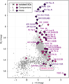 |
Fig. 1 Colour-magnitude diagram displaying the diverse sample of low-and planetary-mass objects observed as part of the ESO SupJup Survey. The pink, circular markers indicate the observed isolated brown dwarfs. The purple hexagons and dark purple diamonds depict the observed companions and their hosts, respectively. As a reference, the photometry of isolated brown dwarfs was obtained from the UltracoolSheet (http://bit.ly/UltracoolSheet) and is used to display late M, L and T dwarfs with increasingly darker marker shades. HR 3549B shows the J – H colour as its K-band magnitude has not been measured. |
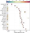 |
Fig. 2 Orbital configuration of the 17 observed bound systems. The systems are ordered by orbital separation (x-axis) of the closest-in observed companion. Marker colours and sizes indicate the spectral types and approximate masses. β Pic c is not filled in since its spectral type is unknown. Transparent symbols denote objects that were not centred on the slit. |
3 DENIS J0255
As a consequence of the similar bulk properties to super-Jupiters, brown dwarfs provide an opportunity to study the atmospheres of planetary-mass objects with high signal-to-noise ratios (S/Ns) due to their proximity to Earth and the absence of contamination from a stellar host. As such, constraints on the atmospheric and chemical properties of brown dwarfs can serve as benchmarks for the study of giant exoplanet atmospheres. Additionally, high-resolution spectra of brown dwarfs and low-mass stars can be used to validate the accuracy and completeness of molecular line lists (e.g. Kesseli et al. 2020; Cont et al. 2021; de Regt et al. 2022; Tannock et al. 2022).
As brown dwarfs age and cool, their atmospheres are subjected to physical and chemical evolution that can be observed in the emergent spectra, colours, and magnitudes (Marley et al. 2010; Charnay et al. 2018). A strong transition occurs between the hotter L-type dwarfs and the cooler T-dwarfs. The late L-dwarfs exhibit redder colours, as is seen in the colour-magnitude diagram of Fig. 1, and present CO absorption in their spectra. At lower temperatures, the T-dwarfs appear bluer and CH4 becomes the dominant carbon-bearing molecule in the observed emission spectra (Cushing et al. 2005). The presence of clouds has commonly been invoked to explain the L-T transition (Allard et al. 2001; Ackerman & Marley 2001; Burrows et al. 2006; Saumon & Marley 2008). These cloud layers would form in the photosphere for L-dwarfs, but recede below it as the temperature decreases towards T-type dwarfs. Alternatively, recent work has suggested that chemical convection could give rise to the transition (Tremblin et al. 2015, 2016). Studying objects near the L-T transition can help to better understand its origin. As such, the field L9-dwarf DENIS J025503.3-470049 offers a prime opportunity to examine the atmospheric processes at the bottom of the L-dwarf branch (Martín et al. 1999; Burgasser et al. 2006). The effective temperature of DENIS J0255 is expected to be Teff ~ 1400 K and its spectrum exhibits signs of a high surface gravity log g ≳ 5 (Cushing et al. 2008; Tremblin et al. 2016; Charnay et al. 2018; Lueber et al. 2022), anticipated for a relatively old brown dwarf (2–4 Gyr from kinematic arguments; Creech-Eakman et al. 2004). Notably, spectroscopic studies at low and moderate resolution have revealed the presence of CH4 absorption (Cushing et al. 2005; Roellig et al. 2004) as well as shallow absorption around ~11 µm which could be attributed to both an NH3 (Creech-Eakman et al. 2004) and a silicate cloud feature (Roellig et al. 2004). Measurements at higher resolving powers revealed a high projected rotational velocity of v sin i ~ 40 km s−1 (Basri et al. 2000; Mohanty & Basri 2003; Zapatero Osorio et al. 2006). Unlike stars, mature brown dwarfs likely retain high rotation rates due to the reduced loss of angular momentum via magnetic winds (Reiners & Basri 2008; Bouvier et al. 2014).
3.1 Observations and reduction
DENIS J0255 was observed on November 2, 2022 as part of the ESO SupJup survey (Program ID: 110.23RW.001, PI: Snellen). The observations were performed in three ABBA nod-cycles, resulting in 12 exposures of 300 s each. As a consequence of its faint R-band magnitude (R ~ 19.9 mag; Costa et al. 2006), Adaptive Optics (AO) could not be used. The K2166 wavelength setting was chosen in order to cover the 13CO bandhead near 2.345 micron (ν = 2–0 transition). The Differential Image Motion Monitor (DIMM) malfunctioned during the observations, but recorded an optical seeing of ~0.7″ and 0.4″ before and after this intermission. These seeing measurements are reasonable assumptions during the observations since the slit viewer camera showed a stable point-spread function. As the seeing was sufficiently low, the spectra were observed with the 0.2″ slit to attain the highest spectral resolution (R = λ/Δλ ~ 100 000). Prior to observing DENIS J0255, observations were made of a telluric standard star, kap Eri, using the same slit, wavelength setting, and also without AO. A single ABBA nod-cycle with 15-s exposures resulted in an S/N of ~240 per pixel near 2.345 µm, which was deemed sufficient to correct for the absorption from the Earth’s atmosphere. The telluric absorption lines were also used to perform a secondary wavelength correction.
The data reduction was carried out with excalibuhr1 (Zhang et al., in prep.,), a Python data reduction pipeline that largely follows the steps outlined in Holmberg & Madhusudhan (2022). excalibuhr employs similar routines as pycrires (Stolker & Landman 2023) and which are also performed with the ESO cr2res pipeline. The exposures were dark-subtracted, flat-fielded, and the background sky emission was removed via subtraction between AB (or BA) nodding pairs. The exposures were subsequently mean-combined per nodding position (i.e. A or B). The evenly spaced lines in the Fabry–Pérot Etalon (FPET) observations were used to extract the slit curvature and served as a first assessment of the wavelength solution. After correcting for the slit curvature and tilt, the spectra were extracted by fitting a profile using the optimal extraction algorithm (Holmberg & Madhusudhan 2022), utilising an extraction aperture of 30 pixels. The 1D spectra at the A and B nodding position were mean-combined and the blaze-function, retrieved from the flat-field exposures, was corrected for. The excalibuhr extraction yielded an S/N of ~40 per pixel at 2.345 µm. The telluric standard spectrum was extracted in a similar manner.
A second-stage wavelength correction was carried out by fitting the telluric standard spectrum to an ESO SkyCalc2 model (Noll et al. 2012; Jones et al. 2013). The initial wavelength solution was stretched and compressed as a third-order polynomial via
 (1)
(1)
where λ′ is the new wavelength solution, pi are the polynomial coefficients, and 〈λ〉 is the average wavelength. The wavelength solution was found separately for each of the seven spectral orders and three detectors via a χ2 -minimisation, employing the Nelder-Mead simplex algorithm implemented in scipy.optimize.minimize (Gao & Han 2012). The telluric standard’s wavelength solution was thereafter adopted for the DENIS J0255 spectrum. As a consequence of its lower S/N and the large number of intrinsic features, the correction could not be performed on the target spectrum directly. However, the wavelength solution is not expected to change considerably as the telluric standard and target were observed in sequence.
The combined telluric transmissivity and instrumental throughput were obtained by dividing the observed, telluric standard spectrum by a PHOENIX model spectrum (Husser et al. 2013). As the high-resolution (R = 500 000) PHOENIX model spectra only go up to an effective temperature of Teff = 12 000 K, we adopted the highest-temperature spectrum and adjusted its slope to match a blackbody spectrum with the temperature of kap Eri (Teff = 14 700 K; Levenhagen & Leister 2006). Any slope error introduced by this correction method is negligible, due to the weak temperature-dependency in the Rayleigh-Jeans regime. The model spectrum was Doppler-shifted to the standard star’s radial velocity (vrad = 25.5 km s−1; Gontcharov 2006) and subsequently broadened to the spectral resolution (R = 100 000) and rotational velocity (v sin i = 10 km s−1; Levenhagen & Leister 2006). This procedure was performed to replicate the line wings of the Brackett γ and δ lines present in the telluric standard’s spectrum. The line cores were more poorly reproduced in the model spectrum, and thus a region of ±1 nm was masked for both lines. The spectrum of DENIS J0255 was subsequently divided by the transmissivity, thereby removing telluric absorption lines and correcting for a wavelength-dependent throughput of the CRIRES+ spectrograph. The deepest telluric lines are saturated and do not provide an adequate correction as a result. Hence, any pixels in which the telluric transmission was lower than 𝒯 < 0.6 were masked in the DENIS J0255 spectrum. A flux-calibration was performed by scaling the observed spectrum to match the 2MASS Ks-band photometry (Ks = 11.56 ± 0.02 mag; Cutri et al. 2003) when integrated over the Ks filter-curve. The utilised Ks-band magnitude was possibly discrepant from the flux at the time of measurement due to the known variability of brown dwarfs, especially at the L–T transition (Wilson et al. 2014; Radigan et al. 2014; Radigan 2014). At least, separate reductions between consecutive nodding pairs showed negligible variability throughout the hour-long observing programme. Residual differences in the observed and calibrating fluxes would be captured by a flux-scaling radius parameter in the retrieval analysis (Sect. 3.2). Finally, outliers were removed by sigma-clipping pixels beyond >3σ from a median-filtered spectrum, using an 8-pixel wide window and the excalibuhr-computed flux-uncertainties as σ. Figure 3 shows the reduced spectrum of DENIS J0255 and a zoom-in of the sixth spectral order in black. The grey line displays the spectrum without correcting for the telluric absorption lines. The evenly spaced spectral lines of 12CO are unmistakably observed in the bottom panel of Fig. 3. The high rotational velocity of DENIS J0255 is also apparent from the line broadening, compared to the narrow telluric lines in grey.
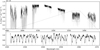 |
Fig. 3 Calibrated spectrum of DENIS J0255, observed with CRIRES+ in the K2166 wavelength setting. The y axes indicate the flux Fλ in units of erg s−1 cm−2 nm−1 and the x axes denote the wavelength λ in nm. Top panel: spectrum over the full wavelength range, with the black line indicating the spectrum after the calibration described in Sect. 3.1. The grey line shows the observed spectrum without correcting for telluric absorption and removing outliers. Bottom panel: zoom-in of the sixth spectral order, presenting numerous rotationally broadened spectral lines of 12CO. |
3.2 Retrieval framework
For the atmospheric retrieval, we employed a Bayesian framework in which the radiative transfer code petitRADTRANS (pRT; Mollière et al. 2019, 2020; Alei et al. 2022) was coupled with the nested sampling tool PyMultiNest (Buchner et al. 2014), which itself is a Python wrapper of the MultiNest algorithm (Feroz et al. 2009). The computations were performed, in parallel, on the Dutch National Supercomputer Snellius3. Model emission spectra were generated by pRT with a number of parameters describing properties such as the thermal profile, chemical abundances, and surface gravity. We defined 50 atmospheric layers between P = 10−6 and 102 bar, equally separated in log pressure. Collision-induced absorption from H2-H2 and H2-He and Rayleigh scattering of H2 and He were taken into account. H2O, 12CO, 13CO, CH4, NH3, CO2, and HCN were included as line opacity species. The HITEMP line lists were employed for 12CO, 13CO (Li et al. 2015), CH4 (Hargreaves et al. 2020), and CO2 (Rothman et al. 2010). ExoMol line lists were used for the opacity of NH3 (Coles et al. 2019) and HCN (Harris et al. 2006; Barber et al. 2014). For H2O, both the ExoMol (POKAZATEL; Polyansky et al. 2018) and HITEMP (Rothman et al. 2010) line lists were evaluated, as is outlined in Sect. 4.4.
While pRT provides an implementation of physically motivated clouds (e.g. MgSiO3, Fe, etc.), we used a simple grey cloud model to not impose any assumptions on the cloud composition. Additionally, this choice was made as we did not expect to constrain any wavelength dependence of the cloud opacity over the covered wavelength range (Δλ ~ 0.5 µm). We implemented the cloud model with the give_absorption_opacity functionality in pRT. Similar to Mollière et al. (2020), the cloud opacity, κcl, at a pressure, P, was computed as
 (2)
(2)
where κcl,0 is the opacity at the cloud base, which is set by Pbase. The cloud opacity decays above the base as a power law controlled by ƒsed. The parameters κcl,0, Pbase, and ƒsed were fit during the retrieval.
The pRT-generated spectra were shifted with a radial velocity, vrad, and subsequently broadened with a projected rotational velocity. v sin i, and linear limb-darkening coefficient, εlimb, using the fastRotBroad routine of PyAstronomy4 (Gray 2008; Czesla et al. 2019). To speed up the computations, the pRT model spectra were generated with an lbl_opacity_sampling = 3 (i.e. R = 106/3). After the rotational broadening, the spectra were down-convolved to a resolution of R = 100 000 to match the 0.2″-slit observations. The observed spectrum might have an increased spectral resolution, resulting from the good seeing (e.g. Lesjak et al. 2023), but the retrieved rotational broadening parameters (v sin i and εlimb) can largely account for any discrepancies.
PyMultiNest samples the parameter space of the relevant free parameters and builds up posterior distributions from repeated likelihood evaluations between the observed and model spectra. Additionally, PyMultiNest computes the Bayesian evidence, 𝒵, and thus allows for model comparisons in which complexity is taken into account (Feroz et al. 2009). The constant efficiency mode was employed to allow for feasible convergence times. Following the MultiNest recommendations5, we used a sampling efficiency of 5% in combination with the importance nested sampling (INS) mode, which allows accurate evidence to be calculated (Feroz et al. 2019). The posterior distribution was sampled with 400 live points and the retrieval terminated with an evidence tolerance of 0.5. For the fiducial model, which consists of a free-chemistry approach, the priors of the retrieved parameters are listed in Table 1. In total, the fiducial retrieval fits for 32 free parameters. The following sections provide further details on the purpose of the listed parameters.
3.2.1 Likelihood and covariance
We adopted a likelihood formalism similar to Gibson et al. (2020). For each order-detector pair, the log-likelihood was calculated as
 (3)
(3)
with N the number of pixels, and Σ0 the covariance matrix, comprising of the flux-uncertainty per pixel and the covariance between the pixels. R denotes the residuals between the observed and model spectrum. Following the linear scaling implementation of Ruffio et al. (2019), the residuals were computed with
 (4)
(4)
where d and m are vectors of the observed and model spectra, respectively. The flux-scaling parameter, ϕ, was optimised for each order and detector except for the first, whose flux was scaled by the free radius parameter, R. Hence, the scaling was performed relative to the first order-detector pair. The rationale behind applying this separate flux-scaling is that it corrects for small, intra-order errors in the slope of the spectrum, possibly introduced by the gain- or blaze-correction. The optimal,  , was found by solving
 (5)
(5)
In Eq. (3), s2 is a covariance scaling parameter that is optimised for each order-detector pair. For the optimally scaled residuals,  was found via
 (6)
(6)
Effectively, the total covariance matrix, Σ = s2Σ0, is scaled so that the reduced chi-squared is equal to  . As a result, s provides an assessment of the over- or underestimation of the flux uncertainties under the assumption of a perfect model fit and when only considering uncorrelated noise. Appendix D of Ruffio et al. (2019) provides more details concerning the method by which the optimal
  are found. Both ϕ and s2 were optimised for each model during the retrieval.
In the case in which the pixel-measurements are uncorre-lated, the covariance matrix would consist only of diagonal, squared uncertainty terms (i.e.  ). However, covari-ance can arise from multiple sources (Czekala et al. 2015; Zhang et al. 2021c; Iyer et al. 2023), including oversampling of the instrumental line spread function by several pixels (~3 pixels for CRIRES+), rotational broadening, systematics, or through imperfections in the model spectrum (e.g. uncertain opacities). Therefore, any deficiencies in a modelled spectral feature result in correlated residuals over multiple adjacent pixels. The retrieved parameters can be biased and their uncertainties will be underestimated when only considering uncorrelated noise. This problem can be addressed by Gaussian processes (GPs), allowing for the modelling of off-diagonal covariance matrix-elements within the Bayesian framework (Czekala et al. 2015; Kawahara et al. 2022). In this work, we employed a global radial basis function (RBF) kernel, similar to Kawahara et al. (2022). The covariance of pixels i and j can then be described as
 (7)
(7)
where δij is the Kronecker delta, and σi the flux-uncertainty of pixel i. Respectively, a and ℓ are the GP amplitude and length-scale, which were sampled as free parameters during the retrieval. The pixel separation, rij, used in this study is given in the velocity space:
 (8)
(8)
with c as the speed of light. The effective uncertainty, σeff,ij, used in this work is given by the arithmetic mean of the variances of pixels i and j:
 (9)
(9)
Thus, the amplitude, a, scales the off-diagonal covariance terms relative to their respective diagonal elements. The GP amplitude, a, was retrieved separately for each order (i.e. a1, a2, etc.), but to minimise the number of free parameters, and since we do not expect the correlation length to differ significantly, we only retrieved one length-scale, ℓ. Correlation between detectors (and orders) was not considered due to the nanometer-wide gaps. We emphasise that the uncertainty scaling parameter, s2, needs to be multiplied with the full Σ0 (in Eq. (3)) to be analytically marginalised over, and thus applies to both components of Eq. (7).
Banded Cholesky decompositions were applied to the covari-ance matrices to compute Eq. (3). The linear algebra of Eqs. (3), (5) and (6) would be computationally expensive because the covariance matrices, Σ0, have considerable sizes per order-detector pair (2048 × 2048 without masking). By the nature of the correlation, the largest values are concentrated near the diagonal. For that reason, only the elements with rij ≤ 51 were considered in the banded Cholesky decomposition, thereby reducing the number of computations to be made. Appendix C presents the results of a retrieval in which the covariance is not modelled and this results in considerable biases to the retrieved parameters.
Free parameters and the utilised prior ranges of the discussed retrievals.
3.2.2 Chemistry
In this work, we considered multiple approaches to modelling the chemical abundances, or volume-mixing ratios (VMRs).
Free-chemistry: The fiducial retrieval consists of a free-chemistry approach, whereby the abundances of relevant chemical species are allowed to vary in order to find the best fit to the data without making assumptions about the thermo-chemical state of the atmosphere. The molecular abundances are kept vertically constant to reduce the number of free parameters. As part of this approach, the He abundance is held constant at VMRHe = 0.15 and the abundance of H2 adjusts to obtain a total VMRtot equal to unity.
Un-quenched equilibrium chemistry: Aside from free-chemistry, the chemical equilibrium implementation of pRT (Mollière et al. 2017) was also tested. With this method, the individual chemical abundances are obtained by interpolating a pre-computed chemical equilibrium table that depends on the pressure, temperature, metallicity ([Fe/H]), and carbon-to-oxygen ratio (C/O). The metallicity and C/O-ratio are retrieved as free parameters in this set-up. In contrast to the free-chemistry approach, the chemical equilibrium abundances are not constant with altitude.
Quenched equilibrium chemistry (Pquench): Additionally, we tested the effect of a simple quenching implementation, whereby we started with the same equilibrium chemistry retrieval as before, but certain molecular abundances were held constant above retrieved quenching pressures, Pquench. Hence, the upper atmosphere was driven out of chemical equilibrium. This assumption of disequilibrium at low pressures can be made since the vertical mixing timescale could become shorter than the chemical reaction timescales of the CO-CH4 and N2-NH3 networks, for example (Visscher & Moses 2011; Zahnle & Marley 2014). Following Zahnle & Marley (2014), we implemented four quenching pressures as retrieved parameters: Pquench(CO, CH4, H2O), Pquench(NH3), Pquench(HCN), and Pquench(CO2), in which the involved molecules are denoted in parentheses.
-
Quenched equilibrium chemistry (Kzz): lastly, Zahnle & Marley (2014) provide prescriptions for the chemical timescales, τchem(P, T, [Fe/H]), of the four aforementioned reaction networks. This allowed us to evaluate the pressures at which the chemical- and mixing timescales are equal, and thus where the quench points are located. For each model, the mixing timescale was calculated as
 (10)
(10)where Kzz, the vertical eddy diffusion coefficient, is a free parameter in this fourth retrieval. The length scale L = αH is defined as the product of the scale height, H, and a factor, α, allowing mixing lengths to be shorter than the scale height, as was found by Smith (1998) and Ackerman & Marley (2001). We adopted α = 1 , so any over-estimation of the length scale, L, would translate into the retrieved Kzz. In comparison to the previous model, this Kzz -retrieval requires a single parameter, rather than four, to describe the quenching.
The differences in the results for the free-chemistry, un-quenched, and quenched equilibrium models are discussed in Sect. 4.3.
3.2.3 Pressure-temperature profile
We present an updated parameterisation of the pressure-temperature (PT) profile, akin to that of Line et al. (2015). A number of knots were defined in pressure space at which the temperatures are retrieved as free parameters. A cubic spline interpolation was subsequently used to determine the temperatures at each of the modelled layers. Depending on the number and spacing of the fitted knots, such a parameterisation can result in unphysical oscillations (e.g. Rowland et al. 2023). A smoothing can be applied to remedy this problem. The Line et al. (2015) parameterisation avoids setting an a priori degree of smoothness by implementing a log-likelihood penalty based on the discrete second derivative of the temperature knots. The penalty is weighted by an additional free parameter, γ, which tunes the smoothing and can allow for more oscillations if the data warrants it.
We first tested the Line et al. (2015) parameterisation, but we encountered some issues. First, the definition of the log-likelihood penalty requires the knots to be spaced equally in log-pressure. Line et al. (2015) chose 15 knots between P = 10−3 and 315 bar to resolve the temperature gradient in the photosphere, but such a large number of free parameters (combined with the parameters for chemistry, cloud structure, etc.) affects the convergence time of MultiNest. In addition, a considerable number of free parameters are used to describe the temperature at pressures above and below the photosphere, which can result in overfitting. Secondly, the log-likelihood penalty is applied to the discrete second derivative in T-log(P) space. In the absence of information, the PT profile will therefore favour a linear solution in T-log(P). However, at low altitudes this is not representative of the convective adiabat of a self-consistent PT profile, which is linear in log(T)–log(P) space. As a result, the PT profile can become too isothermal compared to the convective region of a self-consistent model (e.g. Line et al. 2015, 2017). Applying a penalty to the second derivative in log(T)-log(P) space could offer a solution to this problem, but this can result in temperature gradients that are too steep in the upper atmosphere and photosphere (e.g. Fig. 3 of Rowland et al. 2023). Hence, we decided to penalise the discrete third derivative in log(T)-log(P).
The general P-splines formalism of Li & Cao (2022) was employed to compute the log-likelihood penalty:
 (11)
(11)
where D3 is the third-order general difference matrix, which computes the variations between the temperature knots and weighs them based on their separation in log pressure. Thus, a difference between log(Ti) and log(Ti+1) results in a larger penalty if the node separation is small. Consequently, the knots can be non-uniformly distributed in pressure space, which enables a higher density of knots near the photosphere. In fact, the pressure knots are not required to remain stationary, as long as D3 is re-calculated for each change of node separation. Allowing the knots to vary in temperature as well as pressure can help to avoid a priori assumptions of the location of the photosphere. For that reason, we defined the pressure knots as
 (12)
(12)
where Δ log PPT is the separation between the first and second knots at the bottom of the modelled atmosphere. This value is retrieved as a free parameter (see Table 1), and thus permits the interior knots to shift vertically, towards the photosphere, where the highest resolution is required. To minimise the number of free parameters, the separation between adjacent interior knots was kept constant with an increasing separation as the knots probed the upper atmosphere. In Eq. (11), C is the vector of coefficients that describe the cubic spline interpolation. The method by which D3 and C were computed is outlined in Appendix B.1 and Li & Cao (2022). In Eq. (11), γ is a retrieved, free parameter that scales the contribution of the log-likelihood penalty when it is added to Eq. (3). Contrary to the inverse gamma prior of Line et al. (2015), we imposed a log-uniform prior on γ (see Table 1) because this will similarly favour small values which smooth the PT profile.
The updated PT profile parameterisation was tested on a synthetic spectrum, generated with a Sonora Bobcat PT profile (Marley et al. 2021). The configuration and results of this retrieval are outlined in Appendix B.2. In summary, this PT parameterisation manages to retrieve the input parameters and thermal profile. Hence, we expect to be able to constrain the atmospheric properties of DENIS J0255 from its CRIRES+ spectrum.
4 Results
Figure 4 shows the best-fitting spectrum resulting from the fiducial, free-chemistry retrieval. This fiducial model provides an excellent fit to the data, as is visible from the residuals and the zoom-in of the sixth spectral order. While the residuals are near the level expected from the S/N of the spectrum, Fig. 4 does show some low-order deviations, thereby highlighting the importance of accounting for pixel-to-pixel correlation using GPs. The error bars in Fig. 4 show that the diagonal of the model covariance matrices, Σ, are somewhat reduced compared to the photon noise, except for the reddest order. This indicates an over-estimation of the photon noise by a factor of ~ 1.3. On the other hand, the off-diagonal elements are increased in the modelled covariance. The posterior distributions of constrained parameters and the retrieved thermal profile are shown in Fig. 5. Additionally, the fourth column of Table 1 lists the retrieved values. It should be noted that the retrieved posteriors are likely too narrow, as this is an established issue for MultiNest retrievals (Buchner 2016; Ardévol Martinez et al. 2022; Vasist et al. 2023; Latouf et al. 2023). Our choice of a low sampling efficiency (5%) and constant efficiency mode could contribute to the under-dispersion (Chubb & Min 2022), but this was necessary to achieve reasonable convergence times.
4.1 Bulk properties, temperature, and clouds
Interestingly, within the order-detector pairs, the slope of the K-band spectrum (Canty et al. 2013) provides sufficient information to constrain the surface gravity at log g ~ 5.3, in line with the high surface gravities (log g ≳ 5) found by other studies at lower resolving powers (Cushing et al. 2008; Tremblin et al. 2016; Charnay et al. 2018; Lueber et al. 2022). However, there does exist a weak anti-correlation between log g and v sin i (Pearson correlation: r = −0.20) due to a shared line-broadening effect. The retrieved radius of R ~ 0.8 RJup is consistent with earlier model comparisons as well (Tremblin et al. 2016; Charnay et al. 2018), but we note that this is effectively a retrieval of the 2MASS photometry owing to the basic flux calibration (Sect. 3.1). The rotational and radial velocity measurements also agree with previous work (Basri et al. 2000; Mohanty & Basri 2003; Zapatero Osorio et al. 2006), whereas the retrieved εlimb provides the first assessment of limb-darkening for this brown dwarf. As was expected, the confidence envelopes of the PT profile show tight constraints near the photosphere (0.1–10 bar), indicated by the emission contribution function, and large uncertainties at the higher and lower altitudes which are not probed by the K-band spectrum. The Sonora Bobcat PT profile (orange line; Marley et al. 2021) shown for comparison in Fig. 5 is generally located within the retrieved confidence envelope, signalling an overall agreement with this self-consistent model. The high rotational broadening of DENIS J0255 means that the line cores are shallower and thus do not provide much information about higher altitudes. Hence, on top of the high surface gravity, the emission contribution function is compressed more than it would be for a slowly rotating object. The fiducial model fails to find a solution with a significant grey cloud opacity as κcl ≳ 1 cm2 g−1 is excluded for a cloud base near the photosphere. The validity of this cloud-free solution is discussed in more detail in Sect. 5.1.
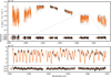 |
Fig. 4 Best-fitting spectrum of the fiducial model, compared to the observed spectrum of DENIS J0255. Upper panels: similar to Fig. 3, the observed spectrum is plotted in black. The orange line displays the model spectrum and the second panel shows the residuals between the observed and model spectra in black. The mean photon noise of each order is indicated with a black error bar. The orange error bar shows the modelled uncertainty, defined as |

4.2 Detection of molecules
The fiducial retrieval finds constraints on the abundances of H2O, 12CO, CH4, NH3, and 13CO; this is presented in Fig. 5. Upper limits are found for the VMRs of CO2 and HCN at 10−6.0 and 10−5.6 (97.5-th percentile), respectively. The retrieved abundances show a strong correlation between species, particularly for H2O, 12CO, and CH4, as is commonly seen for high-resolution spectroscopy (e.g. Gibson et al. 2022; Gandhi et al. 2023b). To determine whether the constraints on CH4, NH3, and 13CO constitute detections, we carried out three additional retrievals with the same set-up as the fiducial model, but we excluded one species at a time. By comparing the Bayesian evidence (𝒵) with that of the fiducial model, we determined to what extent the inclusion of a molecule is favoured. The logarithm of the Bayes factor (Bm), or the difference in log-evidence
 (13)
(13)
was translated into a detection significance following Benneke & Seager (2013). We find that the inclusion of CH4, NH3, and 13CO is favoured at a significance of 23.1σ, 7.9σ, and 2.7σ, respectively.
We also carried out a cross-correlation analysis as a further robustness test of the detections of CH4, NH3, and 13CO. Similar to Zhang et al. (2021b), the cross-correlation function (CCF) was computed between the data residuals; that is, the observed spectrum minus the fiducial model without the opacity from a certain species, and the template for that species. The species’ template was calculated by taking the difference between the complete, fiducial model spectrum, and the fiducial model without that molecule’s opacity, which resulted in the contribution relative to the complete model. The fiducial retrieval was used, rather than the species-excluding retrievals described above, as the latter are likely compensating for the missing opacity by changing the abundance of other species which would result in a spurious cross-correlation signal. The data residuals and species templates were high-pass filtered, using a Gaussian filter with σ = 300 pixels, to remove broad features. At each radial velocity shift, and for each order-detector pair, we computed the cross-correlation coefficient as
 (14)
(14)
where M and R are the high-pass filtered species’ contribution and data residuals, respectively. The cross-correlation was weighted by the non-diagonal covariance matrix, Σ0, thereby placing more importance on separated features. The cross-correlation coefficients of all order-detector pairs were integrated per radial velocity shift. Figure 6 depicts the CCFs for the three considered molecules, in addition to the auto-correlation function (ACF) of the model template. The cross-correlation coefficients were calculated between ±1000 km s−1 in steps of 1 km s−1, in DENIS J0255’s rest frame. In an attempt to limit the effect of auto-correlation, we computed the standard deviation on the residuals of CCF – ACF, excluding the values within −200 < vrad < 200 km s−1. The obtained noise estimate was subsequently used to compute the cross-correlation S/N, which is shown on the right-hand side of Fig. 6. Notably, the CCF of NH3 peaks somewhat to the left of 0 km s−1 ; namely, at −12 km s−1, which might be the result of modelled lines being offset from their true wavelengths. The periodic line structure of 13CO produces the additional lobes observed in its CCF and ACF. The cross-correlation detection significances are established at 30.9σ, 10.6σ, and 3.7σ for CH4, NH3, and 13CO, respectively. From the Bayesian model selection and cross-correlation analyses, we conclude that the presence of CH4 and NH3 is robustly identified, while there is tentative evidence for 13CO.
The constrained 13CO ( ) and 12CO (
 ) abundances translate into an isotopo-logue ratio of
  . The posterior of the carbon isotope ratio, along with the 95% confidence interval, is shown in purple in the bottom right panel of Fig. 7. Section 5.3 provides an interpretation of the 12C/13C-ratio in regard to the possible formation history of DENIS J0255.
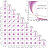 |
Fig. 5 Posterior distributions and thermal structure of DENIS J0255’s atmosphere, retrieved using the fiducial model. Upper right panel: retrieved confidence envelopes of the PT profile. The solid purple line shows the median profile, with the shaded regions showing the 68, 95, and 99.7% confidence intervals. For comparison, a Sonora Bobcat PT profile is shown with an orange line, in addition to condensation curves of several cloud species (MnS: Visscher et al. 2006; MgSiO3, Mg2SiO4, Fe: Visscher et al. 2010). Lower left panels: retrieved physical, chemical, and kinematic parameters and their correlation. The posterior distributions of unconstrained parameters, in addition to those describing the GPs or the PT profile, are omitted for clarity. The vertical dashed lines in the histograms indicate the 16th and 84th percentiles, while the solid line shows the median value. |
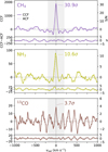 |
Fig. 6 Cross-correlation analysis of CH4, NH3, and 13CO. For each species, the upper panel shows the CCF (solid) and ACF (dashed) with the S/N indicated on the right-hand side. The lower panels present the residuals of CCF-ACF which are used to estimate the noise outside of the expected peak. The cross-correlation was performed on the observed spectrum centred in its rest frame, which resulted in peaks around 0 km s−1. |
4.3 Disequilibrium chemistry
As was described in Sect. 3.2.2, we performed additional retrievals using the pRT chemical equilibrium implementation, both in its quenched and un-quenched form. The retrieval results of the four chemistry approaches are summarised in Table 1 and Fig. 7. The left panel presents the abundance profiles relative to 12CO as high-resolution spectroscopy is most sensitive to abundance ratios.
The results from the Pquench-retrieval show a good agreement with those obtained with the fiducial, free-chemistry model. The emission contribution and PT profile are consistent with the free-chemistry results, but the quenched-chemistry retrieval finds tighter temperature constraints below the photosphere due to its influence on the chemistry at higher altitudes. The CO-CH4 network is quenched at a low altitude ( ), and thus the left panel of Fig. 7 presents almost identical abundances compared to the free-chemistry approach (markers with error bars). The quench point of the N2-NH3 system is placed above that of CO-CH4 (
 ). We note that the photospheric abundance of NH3 is somewhat higher (~0 2 dex) than found in the free-chemistry retrieval. The (median) absolute abundance profiles of 12CO, CH4, H2O, and NH3 are shown as short dashed lines in Fig. 8. The long dashed lines show the behaviour of the abundances if they were left un-quenched (i.e. in chemical equilibrium). At relevant pressures, the un-quenched NH3 abundance profile is never as low as the retrieved free-chemistry abundance. The NH3 quench point is therefore placed at the closest approximation. This discrepancy suggests an elemental nitrogen abundance lower than the solar value assumed for pRT’s chemical equilibrium table. Given the non-detections of HCN and CO2 in the fiducial model, it is not surprising that the respective quenching pressures remain unconstrained. A Bayesian evidence comparison reveals a slight preference for the free-chemistry model at 3.4σ.
Similar results are found with the retrieval implementing quenching via the Kzz -coefficient. The retrieved abundances of CO, CH4, and H2O are in accordance with the free-chemistry and Pquench-retrievals. However, the NH3 mixing ratio is discrepant with the free-chemistry result (~0.2 dex). The pho-tospheric temperature gradient is comparable to the previous models, but higher temperatures are generally retrieved above and below the peak contribution. This can likely be ascribed to the temperature-dependence of the vertical-mixing and chemical timescales. The retrieved  can be converted to quench pressures for the different chemical systems. The derived quench points of the detected species (
 ) are inconsistent with those found in the Pquench-retrieval. Evaluating the Bayes factor reveals a preference (5.3σ) for the free-chemistry model.
The un-quenched equilibrium retrieval is strongly disfavoured over the fiducial retrieval at 29.0σ. The different choices for priors (e.g. log-uniform VMR vs. uniform C/O-ratio) likely decreases the accuracy of the derived significance, but the conclusion that free-chemistry is heavily favoured over un-quenched chemical equilibrium should still hold. Figure 7 shows a PT profile with a minor inversion at the bottom of the photosphere and higher temperatures at altitudes above 10 bar. Moreover, the un-quenched retrieval finds a super-solar metal-licity (![Mathematical equation: $[{\rm{Fe}}/{\rm{H}}] = 0.89_{ - 0.03}^{ + 0.03}$](/articles/aa/full_html/2024/08/aa48508-23/aa48508-23-eq192.png) ), a carbon-to-oxygen ratio (
), a carbon-to-oxygen ratio ( ) that is reduced compared to the quenched- and free-chemistry results, and a surface gravity that hits the edge of the prior (log g ~ 6). These peculiar results are the consequence of attempts to suppress the methane abundance and line depths with respect to 12CO. In the left panel of Fig. 7, we find that the CH4 abundance profile oscillates around the value retrieved with the quenched- and free-chemistry approaches. Maintaining a high temperature will favour CO as the primary carbon-bearing molecule and the retrieval adjusts the emission contribution function via the surface gravity and metallicity. In the absence of these adjustments, methane would become the dominant carbon-bearing molecule (Zahnle & Marley 2014; Moses et al. 2016) as demonstrated in Fig. 8. The short dashed lines indicate the median, quenched abundances profiles and the long dashed lines show the abundances in the absence of quenching (i.e. in chemical equilibrium). We note that these un-quenched profiles are not found with the chemical equilibrium retrieval, as they would produce a poor fit to the observed spectrum. The low temperature between ~ 10−3 and 1 bar would convert CO into CH4 (and H2O) via the net reaction:
 (15)
(15)
However, it is difficult to convert CO into CH4 in reasonable timescales (τchem ~ 108 s at 1 bar and 1250 K; Cooper & Showman 2006) due to its strong triple bond. As a consequence, vertical mixing can retain a CO-rich atmosphere even at low temperatures. The inferred CO and CH4 abundances are therefore evidence of a chemical disequilibrium in the atmosphere of DENIS J0255. The relation between the retrieved disequilibrium and the atmospheric dynamics is discussed in Sect. 5.2.
As shown in the top right panel of Fig. 7, the free-chemistry model obtains a carbon-to-oxygen ratio of  . This atmospheric C/O-ratio might be inflated due to the condensation of oxygen into silicates (Burrows & Sharp 1999; Line et al. 2015; Calamari et al. 2022), which could explain its super-solar value (C/O⊙ = 0.59 ± 0.08; Asplund et al. 2021). The quenched equilibrium models include this oxygen sequestration and thus retrieve lower carbon-to-oxygen ratios (
 ), despite the similar gaseous ratios visible from the relative abundance profiles in the left panel of Fig. 7. While it is more difficult to constrain absolute abundances due to the degeneracies seen in Fig. 5, high-resolution spectroscopy is very sensitive to abundance ratios, and thus results in smaller uncertainties for the C/O-ratio. However, we reiterate that the uncertainties are likely under-estimated due to the chosen constant sampling efficiency of 5% (Chubb & Min 2022). For the free-chemistry model, we employ the carbon abundance relative to hydrogen as a proxy for the atmospheric metallicity. The metallicity retrieved in the free-chemistry (
![Mathematical equation: $[{\rm{C}}/{\rm{H}}] = 0.03_{ - 0.03}^{ + 0.03}$](/articles/aa/full_html/2024/08/aa48508-23/aa48508-23-eq197.png) ) and quenched equilibrium retrievals (
) and quenched equilibrium retrievals (![Mathematical equation: ${[{\rm{Fe}}/{\rm{H}}]_{{\rm{quench }}}} = 0.06_{ - 0.03}^{ + 0.02};{[{\rm{Fe}}/{\rm{H}}]_{{K_z}}} = 0.02_{ - 0.03}^{ + 0.03}$](/articles/aa/full_html/2024/08/aa48508-23/aa48508-23-eq198.png) ) are broadly consistent with the solar measurement, but their difference is observed as a small shift in the absolute abundances of Fig. 8. As depicted in the lower right panel of Fig. 7, the CO isotopologue ratios of the quenched equilibrium models (
) are broadly consistent with the solar measurement, but their difference is observed as a small shift in the absolute abundances of Fig. 8. As depicted in the lower right panel of Fig. 7, the CO isotopologue ratios of the quenched equilibrium models ( ) are in agreement with that of the free-chemistry retrieval (
 ). Evidently, the un-quenched equilibrium model fails to constrain the carbon isotope ratio due to its poor fit to the observed spectrum.
 |
Fig. 7 Retrieval results of three chemistry approaches: free-chemistry (solid/purple), quenched via Pquench (dashed/teal), quenched via Kzz (dot-dashed/turquoise), and un-quenched (dotted/orange) equilibrium chemistry. The line styles are kept consistent in all panels and the envelopes and error bars specify the 95% confidence intervals. Left panel: abundance profiles relative to 12CO for NH3, 13CO, CH4, H2O, and 12CO. The free-chemistry abundances are shown as markers with error bars for clarity, but extend vertically over all pressures. Middle panel: retrieved PT profiles and emission contribution functions. Right panels, from top to bottom: posteriors of the C/O-ratio, metallicity, and carbon isotope ratio. The carbon abundance was used as a proxy for the metallicity (i.e. [C/H]) in the free-chemistry results. The un-quenched equilibrium model finds substantially different results and is heavily disfavoured over the free-chemistry model at 29.0σ. |
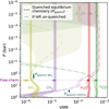 |
Fig. 8 Abundance profiles of 12CO, CH4, H2O, and NH3, retrieved as part of the quenched (via Pquench) chemical equilibrium retrieval. The short dashed lines show the median quenched profiles used to compute the model spectra. For comparison, we show the un-quenched profiles with long dashes, indicating that CH4 would become the dominant carbon-bearing species at pressures below ~1 bar in the case of chemical equilibrium. As in Fig. 7, the shaded regions present the 95% confidence envelopes. |
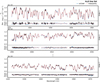 |
Fig. 9 Comparison between the best-fitting model spectra using the HITEMP (blue; Rothman et al. 2010) and ExoMol (orange; Polyansky et al. 2018) line lists for H2O. Only the first, second and seventh spectral orders of the K2166 wavelength setting are shown since the other orders showed minor discrepancies. The residuals of the observed spectrum are shown with respect to the fiducial model which utilises the ExoMol line list. |
4.4 H2O line list validation
High-resolution spectra, like the one analysed in this work, enable reliability tests of the utilised molecular line lists. Accurate and complete line lists improve the robustness of detections of chemical species in exoplanet and brown dwarf atmospheres, as well as improving the modelled abundances, temperature profiles, etc. In this section, we make a comparison between the HITEMP (Rothman et al. 2010) and ExoMol (Polyansky et al. 2018) line lists for H2O. Since ExoMol’s POKAZATEL line list was employed for the fiducial model, a separate retrieval was carried out using the HITEMP line list. Figure 9 presents the difference in best-fitting models for the two bluest and the reddest spectral orders of the K2166 wavelength setting. The four remaining orders showed negligible discrepancies and are therefore not displayed. The HITEMP line list exhibits considerable deviations from the observed spectrum which results in a poor fit in certain regions of orders one, two, and seven. These orders are also the most H2O-dominated at the blue and red edges of the K-band. Furthermore, the Bayesian evidence comparison shows a strong preference for the ExoMol line list at 25.2σ.
As indicated in Table 1, the HITEMP retrieval results are discrepant from those obtained with the fiducial model which uses the ExoMol H2O line list. For instance, the increased GP amplitudes for orders one, two, and seven demonstrate that these wavelength regions are poorly fit as a consequence of inaccurate or incomplete H2O opacities in the HITEMP line list. Moreover, the surface gravity and metallicity are higher in the HITEMP retrieval and it has a shallower temperature gradient. We note that the retrieved isotopologue ratio ( ) is reduced because the retrieval compensates for the inadequate fit with stronger13 CO absorption in the reddest order. Hence, this comparison highlights the importance of accurate line lists for the study of weak features such as isotopologues.
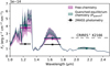 |
Fig. 10 Comparison between the retrieved, cloud-free model spectra and the 2MASS J-, H-, and Ks-band photometry (Cutri et al. 2003). The shaded regions show the 95% confidence intervals. |
5 Discussion
5.1 Validity of cloud-free solution
We find cloud-free solutions for each retrieval, regardless of the employed chemical model. Further tests with the free-chemistry model also failed to detect MgSiO3 or patchy clouds. A possible explanation could be that the fast rotation obscures the continuum by broadening the spectral line wings. This makes it more difficult to probe the cloud layers that are already expected to reside at low altitudes due to the cool temperature of this late L-type object. In the upper right panel of Fig. 5, we show the condensation curves of several cloud species obtained from Visscher et al. (2006, MnS) and Visscher et al. (2010, MgSiO3, Mg2SiO4, Fe). We find that Mg2SiO4 and Fe are presumably condensing out below the K-band photosphere. However, the intersection of the PT profile with the condensation curves of MnS and MgSiO3 suggests that these species could form clouds at pressures probed by the observed CRIRES+ spectrum, but this expected cloud opacity is either negligible or is not sufficiently traced by our grey cloud model. Other retrieval studies of high-resolution K-band spectra have similarly resulted in cloud-free solutions (e.g. Zhang et al. 2021b; Xuan et al. 2022; Landman et al. 2024). The K-band is expected to be less sensitive to clouds than the shorter wavelengths of the J- and H-band. The opacity of gaseous molecules generally increases towards longer wavelengths, leading to higher altitudes becoming probed in the K-band (Marley et al. 2002). Conversely, the opacity of small, sub-micron cloud particles decreases with wavelength (Morley et al. 2014; Marley & Robinson 2015), thereby hampering attempts to constrain the cloud opacity with K-band spectra.
Figure 10 compares the 2MASS J-, H-, and Ks-band photometry (J = 13.25 ± 0.03, H = 12.20 ± 0.02, Ks = 11.56 ± 0.02 mag; Cutri et al. 2003) with the retrieved model spectra, where equilibrium abundances were adopted for FeH, H2S, VO, TiO, K, and Na based on the retrieved C/O-ratio and metallic-ity. We note that the quenched equilibrium retrieval in Fig. 10 shows a narrower flux envelope at shorter wavelengths due to its tighter temperature constraint at low altitudes (see Fig. 7) compared to the free-chemistry results. The model spectra are consistent with the Ks-band photometry on account of the simple flux calibration (Sect. 3.1), but show excess flux in J- and H-band. The true J- and H-band fluxes are likely reduced by clouds that are present below the K-band photosphere and have a decreased opacity at the wavelengths of the CRIRES+ spectrum. As a consequence of the high flux at short wavelengths, we obtain effective temperature estimates of  and
and  for the free-chemistry and quenched equilibrium (Pquench) retrievals, respectively. Evidently, the absence of short-wavelength cloud opacity raises the effective temperature to be inconsistent with the Teff ~ 1400 K found using cloudy models (e.g. Cushing et al. 2008; Charnay et al. 2018; Lueber et al. 2022). Therefore, the lack of constraints on a grey cloud in this work should not be seen as evidence of a cloud-free atmosphere for DENIS J0255 as that would be incompatible with measurements at other wavelengths.
5.2 Chemical quenching and vertical mixing
We find conflicting quench points between the quenched equilibrium retrievals. The Pquench-retrieval quenches the N2–NH3 system above the CO–CH4 quench point. However, for these conditions, the chemical timescale of NH3 is expected to be longer than CO–CH4 and thus vertical mixing should already dominate the N2–NH3 system at lower altitudes (Zahnle & Marley 2014). As discussed in Sect. 4.3, NH3 is quenched at the lowest abundance permitted by the PT profile, leading to the anomalous quench pressure. We find the expected order of quench points in the Kzz-retrieval because the chemical timescale prescription of Zahnle & Marley (2014) was adopted.
Following the method described by Miles et al. (2020) and Xuan et al. (2022), we can convert the constrained quench points from the Pquench-retrieval into vertical eddy diffusion coefficients, Kzz. Since the N2–NH3 network is likely quenched at erroneously high altitudes, we only consider the CO–CH4 system. At the quench point of this network, the chemical reaction timescale ( ; Eq. (14) of Zahnle & Marley 2014) is set equal to the mixing timescale. Using the inverse of Eq. (10), we find an eddy diffusion coefficient of
  (with L = H). For comparison, the directly retrieved diffusion coefficient is constrained about an order of magnitude lower, at
  . However, it is difficult to compare the coefficients as the Kzz-retrieval is also affected by the NH3 abundance that is required to provide a good fit.
Assuming full convection, the upper limit from mixing length theory (Gierasch & Conrath 1985; Zahnle & Marley 2014) is Kzz ≲ 1.1 × 109 cm2 s−1 for DENIS J0255, using Teff = 1400 K and log g = 5.3. Therefore, the inferred  exceeds the upper bound, assuming that the mixing length is equal to the scale height (L = H). For a scaling factor of α = 0.2 (i.e. L = 0.2H), the derived diffusion coefficient
  equals the convective upper limit. Analogous to the analysis presented by Xuan et al. (2022), this suggests that the vertical mixing of DENIS J0255 is primarily driven by efficient convection. The diffusivity derived for DENIS J0255 is similar to that of Xuan et al. (2022) who find Kzz = 5 × 10¹⁰−1 × 1014 cm2 s−1 (L = H) or 5 × 10⁸−1 × 1012 cm2 s−1 (L = 0.1H) for the brown dwarf companion HD 4747B. It is encouraging to find agreement in the inferred Kzz between HD 4747B and DENIS J0255 as the two brown dwarfs share similar effective temperatures, surface gravities, and ages.
In addition to upsetting chemical equilibrium, vertical mixing affects the cloud opacity by transporting condensable vapour upwards to cooler temperatures where condensation can occur. Moreover, vertical mixing counteracts the gravitational settling of cloud particles, and thus allows clouds to be present at higher altitudes (e.g. Ormel & Min 2019; Mukherjee et al. 2022). Hence, the high diffusivity, Kzz, found for DENIS J0255 suggests an increased cloud thickness (Ormel & Min 2019). If our cloud-free solution is truly evidence for the absence of any detectable cloud opacity in the K-band, the obtained eddy diffusion coefficient might help in constraining cloud properties such as the particle sizes. Furthermore, we note that Kzz could decrease with altitude (e.g. Charnay et al. 2018; Tan & Showman 2019; Tan 2022) which might also prevent the clouds from reaching into the probed layers.
5.3 Formation history and isotope ratios
The fiducial, free-chemistry retrieval constrains the CO isotopologue ratio at  . Despite the tentative nature of the 13CO signal, isotope ratios lower than 12C/13C ≲ 97 (0.15th percentile) appear incompatible with the weak 13CO absorption in the observed spectrum. Hence, DENIS J0255 is likely depleted in 13C compared to the local ISM (12C/13C = 68 ± 15; Milam et al. 2005), akin to earlier work for the young brown dwarf 2M 0355 (108 ± 10; Zhang et al. 2021b, 2022) and the fully convective M dwarf binary GJ 745 (296 ± 45, 224 ± 26; Crossfield et al. 2019). A potential explanation for the measured isotopologue ratio is that DENIS J0255 was formed from a parent cloud under-abundant in 13CO, similar to several molecular clouds and young stellar objects in the solar neighbourhood (12C/13C ~ 167; Lambert et al. 1994, ~125; Federman et al. 2003, ~86–158; Goto et al. 2003, ~85–165; Smith et al. 2015). Due to its expected mature age (2-4 Gyr; Creech-Eakman et al. 2004), the parent cloud of DENIS J0255 possibly did not experience considerable 13C-enrichment by asymptotic giant branch stars, in contrast to the present-day ISM (Milam et al. 2005; Romano et al. 2017). With the caveat that 13CO is only weakly identified, this work further supports a possible distinction between the formation pathways of isolated brown dwarfs and super-Jupiters as proposed by Zhang et al. (2021b).
The quenched equilibrium models constrain the isotopologue ratio to  , in line with the ratio found by the free-chemistry model. In contrast, another proposed tracer of planet formation and evolution, the C/O-ratio, results in discrepancies between the models, likely due to the condensation of oxygen into silicate clouds (Burrows & Sharp 1999; Line et al. 2015; Calamari et al. 2022). The similarity in the retrieved 12C/13C-ratios could be an indication that isotope ratios are less sensitive to cloud-condensation and disequilibrium chemistry compared to the C/O-ratio. Such a reduced model dependency forms a good argument for pursuing isotope ratios as tracers of planet formation and evolution.
6 Conclusions
We analysed the high-resolution K-band spectrum of the late L9-dwarf DENIS J0255, observed with CRIRES+ as part of the ESO SupJup Survey. Employing different chemical models in combination with atmospheric retrievals, we find that a free-chemistry approach produces near-identical results to a model in which the chemical equilibrium abundances are quenched above certain altitudes. The retrieval results of an un-quenched equilibrium model are heavily disfavoured at 29.0σ (based on a Bayesian model comparison), thereby unveiling a detection of chemical disequilibrium. In equilibrium, CH4 would be the primary carbon-bearing molecule at the temperature of this brown dwarf, but the long chemical timescales enable DENIS J0255 to retain a CO-rich atmosphere via vertical mixing.
The H2O-dominated edges of the K-band are poorly fit with the HITEMP H2O line list, in contrast to ExoMol’s POKAZA-TEL line list. The Bayesian evidence yields a 25.2σ preference for the ExoMol line list. The comparison reveals discrepancies between the retrieved parameters, and thus emphasises the importance of accurate and complete line lists for reliable results.
A Bayesian evidence comparison shows that the inclusion of CH4, NH3, and the 13CO isotopologue is favoured at a significance of 23.1σ, 7.9σ, and 2.7σ, respectively. A cross-correlation analysis results in detection significances of 30.9σ (CH4), 10.6σ (NH3), and 3.7σ (13CO). Apart from CH4, we report the first confident detection of NH3 in the spectrum of DENIS J0255. The retrieved abundance of the weakly detected 13CO results in an isotopologue ratio of  , while a lower limit of ≳97 can be established. The high ratio suggests that DENIS J0255 is depleted in 13C compared to the present-day, local ISM. Since DENIS J0255 is expected to be several gigayears old, it is expected that its parent cloud was less enriched in 13C from evolved stars. As the second measurement of the CO isotopologue ratio in a brown dwarf’s atmosphere, this paper lends further credence to a possible distinction between the formation pathways of isolated brown dwarfs and super-Jupiters. Future work as part of the ESO SupJup Survey will assess whether depletions of 13C are more commonly seen for these isolated objects and whether the carbon isotope ratio can truly distinguish their formation scenario from that of planetary-mass companions.
Acknowledgements
S.d.R. and I.S. acknowledge funding from the European Research Council (ERC) under the European Union’s Horizon 2020 research and innovation program under grant agreement no. 694513. A.S.L. acknowledges financial support from the Severo Ochoa grant CEX2021-001131-S funded by MCIN/AEI/10.13039/501100011033. T.S. acknowledges the support from the Netherlands Organisation for Scientific Research (NWO) through grant VI.Veni.202.230. This work used the Dutch national e-infrastructure with the support of the SURF Cooperative using grant no. EINF-4556.
Appendix A SupJup observations
Targets observed as part of the ES0 SupJup Survey (Program ID: 1110.C-4264, PI: Sne11en), sorted by right ascension.
Appendix B PT profile parameterisation
B.1 Definition
Here, we describe the method used to compute the general difference matrix D3, following the general, non-uniform P-splines formalism of Li & Cao (2022). As described in Sect. 3.2.3, the spline coefficient vector C is obtained with scipy in log(T)-log(P) space. We employ scipy’s “not-a-knot” method where the third derivative remains continuous over the first and final two segments. Effectively, this removes the second and second-to-last knots from the sequence. However, these knots still influence the spline coefficients in C and their oscillations are still penalised as a result. With a clamped boundary and defining N points in log pressure space, the knots ti are assigned as:
 (B.1)
(B.1)
As described by Li & Cao (2022), the lag-3, lag-2, and lag-1 differences give the diagonal weight matrices W1, W2, W3, respectively. The boundary knots are successively turned “inactive”, so that the weight matrices become
![Mathematical equation: ${{\bf{W}}_1} = {1 \over 3}\left[ {\matrix{ {{t_5} - {t_2}} \hfill & {} \hfill & {} \hfill & {} \hfill & {} \hfill & {} \hfill \cr {} \hfill & {{t_6} - {t_3}} \hfill & {} \hfill & {} \hfill & {} \hfill & {} \hfill \cr {} \hfill & {} \hfill & {{t_7} - {t_4}} \hfill & {} \hfill & {} \hfill & {} \hfill \cr {} \hfill & {} \hfill & {} \hfill & \ddots \hfill & {} \hfill & {} \hfill \cr {} \hfill & {} \hfill & {} \hfill & {} \hfill & {{t_{K - 2}} - {t_{K - 5}}} \hfill & {} \hfill \cr {} \hfill & {} \hfill & {} \hfill & {} \hfill & {} \hfill & {{t_{K - 1}} - {t_{K - 4}}} \hfill \cr } } \right],$](/articles/aa/full_html/2024/08/aa48508-23/aa48508-23-eq222.png) (B.2)
(B.2)
![Mathematical equation: ${W_2} = {1 \over 2}\left[ {\matrix{ {{t_5} - {t_3}} \hfill & {} \hfill & {} \hfill & {} \hfill & {} \hfill & {} \hfill \cr {} \hfill & {{t_6} - {t_4}} \hfill & {} \hfill & {} \hfill & {} \hfill & {} \hfill \cr {} \hfill & {} \hfill & {{t_7} - {t_5}} \hfill & {} \hfill & {} \hfill & {} \hfill \cr {} \hfill & {} \hfill & {} \hfill & \ddots \hfill & {} \hfill & {} \hfill \cr {} \hfill & {} \hfill & {} \hfill & {} \hfill & {{t_{K - 3}} - {t_{K - 5}}} \hfill & {} \hfill \cr {} \hfill & {} \hfill & {} \hfill & {} \hfill & {} \hfill & {{t_{K - 2}} - {t_{K - 4}}} \hfill \cr } } \right],$](/articles/aa/full_html/2024/08/aa48508-23/aa48508-23-eq223.png) (B.3)
(B.3)
![Mathematical equation: ${W_3} = {1 \over 1}\left[ {\matrix{ {{t_5} - {t_4}} \hfill & {} \hfill & {} \hfill & {} \hfill & {} \hfill & {} \hfill \cr {} \hfill & {{t_6} - {t_5}} \hfill & {} \hfill & {} \hfill & {} \hfill & {} \hfill \cr {} \hfill & {} \hfill & {{t_7} - {t_6}} \hfill & {} \hfill & {} \hfill & {} \hfill \cr {} \hfill & {} \hfill & {} \hfill & \ddots \hfill & {} \hfill & {} \hfill \cr {} \hfill & {} \hfill & {} \hfill & {} \hfill & {{t_{K - 3}} - {t_{K - 5}}} \hfill & {} \hfill \cr {} \hfill & {} \hfill & {} \hfill & {} \hfill & {} \hfill & {{t_{K - 3}} - {t_{K - 4}}} \hfill \cr } } \right].$](/articles/aa/full_html/2024/08/aa48508-23/aa48508-23-eq224.png) (B.4)
(B.4)
The fundamental difference matrix is defined as
![Mathematical equation: $\Delta = \left[ {\matrix{ { - 1} & 1 & {} & {} & {} \cr {} & { - 1} & 1 & {} & {} \cr {} & {} & \ddots & \ddots & {} \cr {} & {} & {} & { - 1} & 1 \cr } } \right],$](/articles/aa/full_html/2024/08/aa48508-23/aa48508-23-eq225.png) (B.5)
(B.5)
where its exact dimensions alter, depending on the calculation performed. These matrices are used to compute the variation between coefficients in the vector C as ΔC. Consecutively performing this difference computation and weighting by the inverse of Wi results in the first-, second- and third-order general differences:
 (B.6)
(B.6)
 (B.7)
(B.7)
 (B.8)
(B.8)
where D3 is the third-order general difference matrix. The third-order general difference penalty is then calculated as the squared norm of the general difference:
 (B.9)
(B.9)
B.2 Retrieval of synthetic spectrum
To verify the applicability of the updated PT parameterisation, we use a synthetic spectrum to evaluate the retrieval of its input parameters. As the input PT profile, we employ a Sonora Bobcat profile (Marley et al. 2021) with an effective temperature of Teff = 1400 K, surface gravity log g = 5.25, solar metallicity and solar C/O-ratio (Cushing et al. 2008; Tremblin et al. 2016; Charnay et al. 2018; Lueber et al. 2022). Furthermore, we adopt R = 0.8 RJup, log 12CO = −3.3, log 13CO = −5.5, log H2O = −3.6, log CH4 = −4.9, log NH3 = −6.0, εlimb = 0.65, v sin i = 41.0 km s−1, and vrad = 22.5 km s−1 (Basri et al. 2000; Mohanty & Basri 2003; Zapatero Osorio et al. 2006). After generating a pRT spectrum with these parameters, the spectrum is convolved down to the CRIRES+ spectral resolving power (R ~ 100 000). Similar to the observed spectrum, pixels are masked where deep tellurics exist. Gaussian noise is added to the synthetic spectrum by using the flux uncertainties of the observed spectrum of DENIS J0255. For the retrieval on this synthetic spectrum, we use the same priors as the fiducial model (see Table 1) except for the cloud and GP parameters, which are not retrieved.
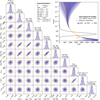 |
Fig. B.1 Posterior distributions retrieved from the synthetic spectrum. The orange lines denote the input parameters and PT profile, which are compatible with the retrieval within the 95% credible region. Following the Schwarzschild criterion, the radiative-convective boundary (RCB) is indicated with a point near 10 bar and 1800 K. |
The results of the retrieval are presented in Fig. B.1. The retrieved posterior distributions are compatible with the input parameters, indicated by orange lines, within the 95% confidence interval. As a known deficiency of the MultiNest algorithm, the sampled posteriors are likely under-dispersed (e.g. Buchner 2016; Ardévol Martinez et al. 2022; Chubb & Min 2022; Vasist et al. 2023, Latouf et al. 2023), which might explain the offset of the retrieved radial velocity. Below the photosphere, we observe that the retrieved PT envelope is somewhat steeper than the input Sonora Bobcat profile. The synthetic spectrum provides negligible information about this region of the atmosphere, and thus results in a PT envelope that covers the given prior, albeit smoothened by the third-order general difference penalty. Inside the photosphere, the Sonora Bobcat PT profile is almost perfectly recovered. Therefore, we expect that the updated PT profile parameterisation is well applicable to the observed CRIRES+ spectrum and should be capable of constraining the atmospheric properties of DENIS J0255.
Appendix C Gaussian processes
To demonstrate the importance of modelling the off-diagonal covariance elements, we carry out a retrieval without GPs. Apart from the GP parameters, we utilise the same priors as the fiducial model (see Table 1). We note that the optimal covariance scaling parameter  is still calculated, but is different from the fiducial model as it only scales the flux-uncertainties. The posterior distributions of the retrieval without GPs is shown in red in Fig. C.1 and compared to the fiducial retrieval results in pink. Since introducing GPs effectively smoothens out the likelihood landscape, the results without GPs show narrower posteriors and smaller uncertainties. Moreover, the retrieved values are substantially biased if covariance is not accounted for. For example, a large temperature inversion is constrained at ~10−4 bar in order to make the deepest H2O lines more shallow at the K-band edges. This inversion is the result of overfitting as these lines are also well-reproduced by the fiducial model (see Fig. 9). Similarly, we find a radius and surface gravity discrepant from the results obtained in the fiducial retrieval. In spite of some minor offsets in the abundances, the corresponding carbon-to-oxygen ratio
  , metallicity
 ![Mathematical equation: $[{\rm{C}}/{\rm{H}}] = 0.05_{ - 0.01}^{ + 0.01}$](/articles/aa/full_html/2024/08/aa48508-23/aa48508-23-eq232.png) , and carbon isotope ratio
, and carbon isotope ratio  are still compatible with those found with the fiducial model. The discrepancies between retrievals with and without covariance modelling are expected to be smaller for spectra that experience less rotational broadening than DENIS J0255 (v sin i ~ 41 km s−1), considering the reduced correlation between adjacent pixels.
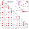 |
Fig. C.1 Comparison between the retrieval results of a model without GPs (red) and the fiducial model (pink). The values shown above each 1D histogram provide the median and 68% confidence interval of the retrieval without GPs. The thermal inversion in the upper right panel and the narrow and biased posteriors in the lower left panels are the result of overfitting when covariance is not modelled. |
References
- Ackerman, A. S., & Marley, M. S. 2001, ApJ, 556, 872 [Google Scholar]
- Alarcón, F., Teague, R., Zhang, K., Bergin, E. A., & Barraza-Alfaro, M. 2020, ApJ, 905, 68 [Google Scholar]
- Alday, J., Trokhimovskiy, A., Irwin, P. G. J., et al. 2021, Nat. Astron., 5, 943 [NASA ADS] [CrossRef] [Google Scholar]
- Alei, E., Konrad, B. S., Angerhausen, D., et al. 2022, A&A, 665, A106 [NASA ADS] [CrossRef] [EDP Sciences] [Google Scholar]
- Allard, F., Hauschildt, P. H., Alexander, D. R., Tamanai, A., & Schweitzer, A. 2001, ApJ, 556, 357 [Google Scholar]
- Allers, K. N., & Liu, M. C. 2013, ApJ, 772, 79 [NASA ADS] [CrossRef] [Google Scholar]
- Ardévol Martínez, F., Min, M., Kamp, I., & Palmer, P. I. 2022, A&A, 662, A108 [NASA ADS] [CrossRef] [EDP Sciences] [Google Scholar]
- Artigau, É., Gagné, J., Faherty, J., et al. 2015, ApJ, 806, 254 [NASA ADS] [CrossRef] [Google Scholar]
- Asplund, M., Amarsi, A. M., & Grevesse, N. 2021, A&A, 653, A141 [NASA ADS] [CrossRef] [EDP Sciences] [Google Scholar]
- Barber, R. J., Strange, J. K., Hill, C., et al. 2014, MNRAS, 437, 1828 [CrossRef] [Google Scholar]
- Bardalez Gagliuffi, D. C., Burgasser, A. J., Gelino, C. R., et al. 2014, ApJ, 794, 143 [NASA ADS] [CrossRef] [Google Scholar]
- Basri, G., Mohanty, S., Allard, F., et al. 2000, ApJ, 538, 363 [NASA ADS] [CrossRef] [Google Scholar]
- Bell, C. P. M., Mamajek, E. E., & Naylor, T. 2015, MNRAS, 454, 593 [Google Scholar]
- Benneke, B., & Seager, S. 2013, ApJ, 778, 153 [Google Scholar]
- Biller, B. A., Liu, M. C., Wahhaj, Z., et al. 2010, ApJ, 720, L82 [NASA ADS] [CrossRef] [Google Scholar]
- Birkby, J. L. 2018, in Handbook of Exoplanets, eds. H. J. Deeg, & J. A. Belmonte, 16 [Google Scholar]
- Bohn, A. J., Kenworthy, M. A., Ginski, C., et al. 2020a, MNRAS, 492, 431 [Google Scholar]
- Bohn, A. J., Kenworthy, M. A., Ginski, C., et al. 2020b, ApJ, 898, L16 [Google Scholar]
- Bonnefoy, M., Chauvin, G., Rojo, P., et al. 2010, A&A, 512, A52 [NASA ADS] [CrossRef] [EDP Sciences] [Google Scholar]
- Booth, M., del Burgo, C., & Hambaryan, V. V. 2021, MNRAS, 500, 5552 [Google Scholar]
- Bouvier, J., Matt, S. P., Mohanty, S., et al. 2014, in Protostars and Planets VI, eds. H. Beuther, R. S. Klessen, C. P. Dullemond, & T. Henning, 433 [Google Scholar]
- Bowler, B. P., Liu, M. C., Shkolnik, E. L., & Dupuy, T. J. 2013, ApJ, 774, 55 [NASA ADS] [CrossRef] [Google Scholar]
- Bowler, B. P., Kraus, A. L., Bryan, M. L., et al. 2017, AJ, 154, 165 [Google Scholar]
- Brogi, M., Snellen, I. A. G., de Kok, R. J., et al. 2012, Nature, 486, 502 [Google Scholar]
- Brogi, M., de Kok, R. J., Albrecht, S., et al. 2016, ApJ, 817, 106 [Google Scholar]
- Brogi, M., Line, M., Bean, J., Désert, J. M., & Schwarz, H. 2017, ApJ, 839, L2 [Google Scholar]
- Buchner, J. 2016, Statist. Comput., 26, 383 [NASA ADS] [CrossRef] [Google Scholar]
- Buchner, J., Georgakakis, A., Nandra, K., et al. 2014, A&A, 564, A125 [NASA ADS] [CrossRef] [EDP Sciences] [Google Scholar]
- Burgasser, A. J., Geballe, T. R., Leggett, S. K., Kirkpatrick, J. D., & Golimowski, D. A. 2006, ApJ, 637, 1067 [Google Scholar]
- Burgasser, A. J., Sheppard, S. S., & Luhman, K. L. 2013, ApJ, 772, 129 [Google Scholar]
- Burrows, A., & Sharp, C. M. 1999, ApJ, 512, 843 [NASA ADS] [CrossRef] [Google Scholar]
- Burrows, A., Sudarsky, D., & Hubeny, I. 2006, ApJ, 640, 1063 [Google Scholar]
- Calamari, E., Faherty, J. K., Burningham, B., et al. 2022, ApJ, 940, 164 [NASA ADS] [CrossRef] [Google Scholar]
- Canty, J. I., Lucas, P. W., Roche, P. F., & Pinfield, D. J. 2013, MNRAS, 435, 2650 [NASA ADS] [CrossRef] [Google Scholar]
- Charnay, B., Bézard, B., Baudino, J. L., et al. 2018, ApJ, 854, 172 [Google Scholar]
- Chauvin, G., Lagrange, A. M., Zuckerman, B., et al. 2005, A&A, 438, L29 [NASA ADS] [CrossRef] [EDP Sciences] [Google Scholar]
- Cheetham, A., Bonnefoy, M., Desidera, S., et al. 2018, A&A, 615, A160 [NASA ADS] [CrossRef] [EDP Sciences] [Google Scholar]
- Chilcote, J., Pueyo, L., De Rosa, R. J., et al. 2017, AJ, 153, 182 [Google Scholar]
- Chubb, K. L., & Min, M. 2022, A&A, 665, A2 [NASA ADS] [CrossRef] [EDP Sciences] [Google Scholar]
- Clayton, D. D., & Nittler, L. R. 2004, ARA&A, 42, 39 [NASA ADS] [CrossRef] [Google Scholar]
- Coles, P. A., Yurchenko, S. N., & Tennyson, J. 2019, MNRAS, 490, 4638 [CrossRef] [Google Scholar]
- Cont, D., Yan, F., Reiners, A., et al. 2021, A&A, 651, A33 [NASA ADS] [CrossRef] [EDP Sciences] [Google Scholar]
- Cooper, C. S., & Showman, A. P. 2006, ApJ, 649, 1048 [CrossRef] [Google Scholar]
- Costa, E., Méndez, R. A., Jao, W. C., et al. 2006, AJ, 132, 1234 [CrossRef] [Google Scholar]
- Creech-Eakman, M. J., Orton, G. S., Serabyn, E., & Hayward, T. L. 2004, ApJ, 602, L129 [NASA ADS] [CrossRef] [Google Scholar]
- Cridland, A. J., Pudritz, R. E., & Alessi, M. 2016, MNRAS, 461, 3274 [Google Scholar]
- Crossfield, I. J. M., Lothringer, J. D., Flores, B., et al. 2019, ApJ, 871, L3 [NASA ADS] [CrossRef] [Google Scholar]
- Cruz, K. L., Reid, I. N., Liebert, J., Kirkpatrick, J. D., & Lowrance, P. J. 2003, AJ, 126, 2421 [Google Scholar]
- Cruz, K. L., Kirkpatrick, J. D., & Burgasser, A. J. 2009, AJ, 137, 3345 [NASA ADS] [CrossRef] [Google Scholar]
- Cushing, M. C., Rayner, J. T., & Vacca, W. D. 2005, ApJ, 623, 1115 [Google Scholar]
- Cushing, M. C., Marley, M. S., Saumon, D., et al. 2008, ApJ, 678, 1372 [NASA ADS] [CrossRef] [Google Scholar]
- Cutri, R. M., Skrutskie, M. F., van Dyk, S., et al. 2003, VizieR Online Data Catalog: II/246 [Google Scholar]
- Czekala, I., Andrews, S. M., Mandel, K. S., Hogg, D. W., & Green, G. M. 2015, ApJ, 812, 128 [NASA ADS] [CrossRef] [Google Scholar]
- Czesla, S., Schröter, S., Schneider, C. P., et al. 2019, PyA: Python astronomy-related packages, Astrophysics Source Code Library [record ascl:1906.010] [Google Scholar]
- de Regt, S., Kesseli, A. Y., Snellen, I. A. G., Merritt, S. R., & Chubb, K. L. 2022, A&A, 661, A109 [NASA ADS] [CrossRef] [EDP Sciences] [Google Scholar]
- Delorme, P., Gagné, J., Girard, J. H., et al. 2013, A&A, 553, A5 [Google Scholar]
- Dorn, R. J., Anglada-Escude, G., Baade, D., et al. 2014, The Messenger, 156, 7 [NASA ADS] [Google Scholar]
- Dorn, R. J., Bristow, P., Smoker, J. V., et al. 2023, A&A, 671, A24 [NASA ADS] [CrossRef] [EDP Sciences] [Google Scholar]
- Ehrenreich, D., Lovis, C., Allart, R., et al. 2020, Nature, 580, 597 [Google Scholar]
- Faherty, J. K., Burgasser, A. J., West, A. A., et al. 2010, AJ, 139, 176 [NASA ADS] [CrossRef] [Google Scholar]
- Faherty, J. K., Riedel, A. R., Cruz, K. L., et al. 2016, ApJS, 225, 10 [Google Scholar]
- Federman, S. R., Lambert, D. L., Sheffer, Y., et al. 2003, ApJ, 591, 986 [NASA ADS] [CrossRef] [Google Scholar]
- Feroz, F., Hobson, M. P., & Bridges, M. 2009, MNRAS, 398, 1601 [NASA ADS] [CrossRef] [Google Scholar]
- Feroz, F., Hobson, M. P., Cameron, E., & Pettitt, A. N. 2019, Open J. Astrophys., 2, 10 [Google Scholar]
- Feuchtgruber, H., Lellouch, E., Orton, G., et al. 2013, A&A, 551, A126 [NASA ADS] [CrossRef] [EDP Sciences] [Google Scholar]
- Franson, K., & Bowler, B. P. 2023, AJ, 165, 246 [NASA ADS] [CrossRef] [Google Scholar]
- Gagné, J., Faherty, J. K., Cruz, K. L., et al. 2015, ApJS, 219, 33 [CrossRef] [Google Scholar]
- Gagné, J., Mamajek, E. E., Malo, L., et al. 2018, ApJ, 856, 23 [Google Scholar]
- Gaia Collaboration 2020, VizieR Online Data Catalog: I/350 [Google Scholar]
- Gandhi, S., de Regt, S., Snellen, I., et al. 2023a, ApJ, 957, L36 [NASA ADS] [CrossRef] [Google Scholar]
- Gandhi, S., Kesseli, A., Zhang, Y., et al. 2023b, AJ, 165, 242 [NASA ADS] [CrossRef] [Google Scholar]
- Gao, F., & Han, L. 2012, Comput. Optim. Applic., 51, 259 [Google Scholar]
- Garcia, E. V., Currie, T., Guyon, O., et al. 2017, ApJ, 834, 162 [NASA ADS] [CrossRef] [Google Scholar]
- Geballe, T. R., Knapp, G. R., Leggett, S. K., et al. 2002, ApJ, 564, 466 [Google Scholar]
- Giacobbe, P., Brogi, M., Gandhi, S., et al. 2021, Nature, 592, 205 [NASA ADS] [CrossRef] [Google Scholar]
- Gibson, N. P., Merritt, S., Nugroho, S. K., et al. 2020, MNRAS, 493, 2215 [Google Scholar]
- Gibson, N. P., Nugroho, S. K., Lothringer, J., Maguire, C., & Sing, D. K. 2022, MNRAS, 512, 4618 [NASA ADS] [CrossRef] [Google Scholar]
- Gierasch, P. J., & Conrath, B. J. 1985, in Recent Advances in Planetary Meteorology, ed. G. E. Hunt, 121 [Google Scholar]
- Gizis, J. E. 2002, ApJ, 575, 484 [NASA ADS] [CrossRef] [Google Scholar]
- Gontcharov, G. A. 2006, Astron. Lett., 32, 759 [Google Scholar]
- Goto, M., Usuda, T., Takato, N., et al. 2003, ApJ, 598, 1038 [NASA ADS] [CrossRef] [Google Scholar]
- GRAVITY Collaboration (Nowak, M., et al.) 2020, A&A, 633, A110 [NASA ADS] [CrossRef] [EDP Sciences] [Google Scholar]
- Gray, D. F. 2008, The Observation and Analysis of Stellar Photospheres (Cambridge, UK: Cambridge University) [Google Scholar]
- Hargreaves, R. J., Gordon, I. E., Rey, M., et al. 2020, ApJS, 247, 55 [NASA ADS] [CrossRef] [Google Scholar]
- Harris, G. J., Tennyson, J., Kaminsky, B. M., Pavlenko, Y. V., & Jones, H. R. A. 2006, MNRAS, 367, 400 [Google Scholar]
- Herbig, G. H. 1977, ApJ, 214, 747 [Google Scholar]
- Hoeijmakers, H. J., Seidel, J. V., Pino, L., et al. 2020, A&A, 641, A123 [NASA ADS] [CrossRef] [EDP Sciences] [Google Scholar]
- Holmberg, M., & Madhusudhan, N. 2022, AJ, 164, 79 [NASA ADS] [CrossRef] [Google Scholar]
- Husser, T. O., Wende-von Berg, S., Dreizler, S., et al. 2013, A&A, 553, A6 [NASA ADS] [CrossRef] [EDP Sciences] [Google Scholar]
- Itoh, Y., Hayashi, M., Tamura, M., et al. 2005, ApJ, 620, 984 [NASA ADS] [CrossRef] [Google Scholar]
- Iyer, A. R., Line, M. R., Muirhead, P. S., Fortney, J. J., & Gharib-Nezhad, E. 2023, ApJ, 944, 41 [NASA ADS] [CrossRef] [Google Scholar]
- Jenkins, J. S., Pavlenko, Y. V., Ivanyuk, O., et al. 2012, MNRAS, 420, 3587 [NASA ADS] [Google Scholar]
- Jones, A., Noll, S., Kausch, W., Szyszka, C., & Kimeswenger, S. 2013, A&A, 560, A91 [NASA ADS] [CrossRef] [EDP Sciences] [Google Scholar]
- Kaeufl, H.-U., Ballester, P., Biereichel, P., et al. 2004, SPIE Conf. Ser., 5492, 1218 [NASA ADS] [Google Scholar]
- Kawahara, H., Kawashima, Y., Masuda, K., et al. 2022, ApJS, 258, 31 [NASA ADS] [CrossRef] [Google Scholar]
- Kenyon, S. J., & Hartmann, L. 1995, ApJS, 101, 117 [Google Scholar]
- Kesseli, A. Y., Snellen, I. A. G., Alonso-Floriano, F. J., Mollière, P., & Serindag, D. B. 2020, AJ, 160, 228 [NASA ADS] [CrossRef] [Google Scholar]
- Kraus, A. L., Ireland, M. J., Cieza, L. A., et al. 2014, ApJ, 781, 20 [Google Scholar]
- Kulikov, Y. N., Lammer, H., Lichtenegger, H. I. M., et al. 2006, Planet. Space Sci., 54, 1425 [NASA ADS] [CrossRef] [Google Scholar]
- Lacour, S., Wang, J. J., Rodet, L., et al. 2021, A&A, 654, A2 [NASA ADS] [CrossRef] [EDP Sciences] [Google Scholar]
- Lambert, D. L., Sheffer, Y., Gilliland, R. L., & Federman, S. R. 1994, ApJ, 420, 756 [NASA ADS] [CrossRef] [Google Scholar]
- Landman, R., Stolker, T., Snellen, I. A. G., et al. 2024, A&A, 682, A48 [NASA ADS] [CrossRef] [EDP Sciences] [Google Scholar]
- Langer, W. D., & Penzias, A. A. 1993, ApJ, 408, 539 [NASA ADS] [CrossRef] [Google Scholar]
- Latouf, N., Mandell, A. M., Villanueva, G. L., et al. 2023, AJ, 166, 129 [NASA ADS] [CrossRef] [Google Scholar]
- Lavigne, J.-F., Doyon, R., Lafrenière, D., Marois, C., & Barman, T. 2009, ApJ, 704, 1098 [Google Scholar]
- Lazorenko, P. F., & Sahlmann, J. 2018, A&A, 618, A111 [NASA ADS] [CrossRef] [EDP Sciences] [Google Scholar]
- Lesjak, F., Nortmann, L., Yan, F., et al. 2023, A&A, 678, A23 [NASA ADS] [CrossRef] [EDP Sciences] [Google Scholar]
- Levenhagen, R. S., & Leister, N. V. 2006, MNRAS, 371, 252 [Google Scholar]
- Li, Z., & Cao, J. 2022, arXiv e-prints [arXiv:2201.86808] [Google Scholar]
- Li, G., Gordon, I. E., Rothman, L. S., et al. 2015, ApJS, 216, 15 [NASA ADS] [CrossRef] [Google Scholar]
- Line, M. R., Teske, J., Burningham, B., Fortney, J. J., & Marley, M. S. 2015, ApJ, 807, 183 [NASA ADS] [CrossRef] [Google Scholar]
- Line, M. R., Marley, M. S., Liu, M. C., et al. 2017, ApJ, 848, 83 [NASA ADS] [CrossRef] [Google Scholar]
- Line, M. R., Brogi, M., Bean, J. L., et al. 2021, Nature, 598, 580 [NASA ADS] [CrossRef] [Google Scholar]
- Lothringer, J. D., Rustamkulov, Z., Sing, D. K., et al. 2021, ApJ, 914, 12 [CrossRef] [Google Scholar]
- Lowrance, P. J., McCarthy, C., Becklin, E. E., et al. 1999, ApJ, 512, L69 [NASA ADS] [CrossRef] [Google Scholar]
- Lueber, A., Kitzmann, D., Bowler, B. P., Burgasser, A. J., & Heng, K. 2022, ApJ, 930, 136 [NASA ADS] [CrossRef] [Google Scholar]
- Luhman, K. L. 2013, ApJ, 767, L1 [NASA ADS] [CrossRef] [Google Scholar]
- Luhman, K. L., Wilson, J. C., Brandner, W., et al. 2006, ApJ, 649, 894 [NASA ADS] [CrossRef] [Google Scholar]
- Luhman, K. L., Mamajek, E. E., Allen, P. R., Muench, A. A., & Finkbeiner, D. P. 2009, ApJ, 691, 1265 [NASA ADS] [CrossRef] [Google Scholar]
- MacGregor, M. A., Wilner, D. J., Czekala, I., et al. 2017, ApJ, 835, 17 [Google Scholar]
- Madhusudhan, N. 2012, ApJ, 758, 36 [NASA ADS] [CrossRef] [Google Scholar]
- Maire, A. L., Bonnefoy, M., Ginski, C., et al. 2016, A&A, 587, A56 [NASA ADS] [CrossRef] [EDP Sciences] [Google Scholar]
- Marley, M. S., & Robinson, T. D. 2015, ARA&A, 53, 279 [Google Scholar]
- Marley, M. S., Seager, S., Saumon, D., et al. 2002, ApJ, 568, 335 [NASA ADS] [CrossRef] [Google Scholar]
- Marley, M. S., Saumon, D., & Goldblatt, C. 2010, ApJ, 723, L117 [NASA ADS] [CrossRef] [Google Scholar]
- Marley, M. S., Saumon, D., Cushing, M., et al. 2012, ApJ, 754, 135 [Google Scholar]
- Marley, M. S., Saumon, D., Visscher, C., et al. 2021, ApJ, 920, 85 [NASA ADS] [CrossRef] [Google Scholar]
- Martín, E. L., Delfosse, X., Basri, G., et al. 1999, AJ, 118, 2466 [Google Scholar]
- Mawet, D., David, T., Bottom, M., et al. 2015, ApJ, 811, 103 [NASA ADS] [CrossRef] [Google Scholar]
- McGovern, M. R., Kirkpatrick, J. D., McLean, I. S., et al. 2004, ApJ, 600, 1020 [NASA ADS] [CrossRef] [Google Scholar]
- Mesa, D., Vigan, A., D’Orazi, V., et al. 2016, A&A, 593, A119 [NASA ADS] [CrossRef] [EDP Sciences] [Google Scholar]
- Mesa, D., D’Orazi, V., Vigan, A., et al. 2020, MNRAS, 495, 4279 [Google Scholar]
- Milam, S. N., Savage, C., Brewster, M. A., Ziurys, L. M., & Wyckoff, S. 2005, ApJ, 634, 1126 [Google Scholar]
- Miles, B. E., Skemer, A. J. I., Morley, C. V., et al. 2020, AJ, 160, 63 [NASA ADS] [CrossRef] [Google Scholar]
- Mohanty, S., & Basri, G. 2003, ApJ, 583, 451 [NASA ADS] [CrossRef] [Google Scholar]
- Mollière, P., & Snellen, I. A. G. 2019, A&A, 622, A139 [NASA ADS] [CrossRef] [EDP Sciences] [Google Scholar]
- Mollière, P., van Boekel, R., Bouwman, J., et al. 2017, A&A, 600, A10 [Google Scholar]
- Mollière, P., Wardenier, J. P., van Boekel, R., et al. 2019, A&A, 627, A67 [Google Scholar]
- Mollière, P., Stolker, T., Lacour, S., et al. 2020, A&A, 640, A131 [Google Scholar]
- Mollière, P., Molyarova, T., Bitsch, B., et al. 2022, ApJ, 934, 74 [CrossRef] [Google Scholar]
- Monin, J. L., Guieu, S., Pinte, C., et al. 2010, A&A, 515, A91 [NASA ADS] [CrossRef] [EDP Sciences] [Google Scholar]
- Mordasini, C., van Boekel, R., Mollière, P., Henning, T., & Benneke, B. 2016, ApJ, 832, 41 [Google Scholar]
- Morley, C. V., Marley, M. S., Fortney, J. J., et al. 2014, ApJ, 787, 78 [Google Scholar]
- Moses, J. I., Marley, M. S., Zahnle, K., et al. 2016, ApJ, 829, 66 [Google Scholar]
- Mukherjee, S., Fortney, J. J., Batalha, N. E., et al. 2022, ApJ, 938, 107 [NASA ADS] [CrossRef] [Google Scholar]
- Murphy, S. J., Lawson, W. A., & Bessell, M. S. 2013, MNRAS, 435, 1325 [Google Scholar]
- Neuhäuser, R., Schmidt, T. O. B., Hambaryan, V. V., & Vogt, N. 2010, A&A, 516, A112 [NASA ADS] [CrossRef] [EDP Sciences] [Google Scholar]
- Nielsen, E. L., Liu, M. C., Wahhaj, Z., et al. 2012, ApJ, 750, 53 [Google Scholar]
- Noll, S., Kausch, W., Barden, M., et al. 2012, A&A, 543, A92 [NASA ADS] [CrossRef] [EDP Sciences] [Google Scholar]
- Öberg, K. I., Murray-Clay, R., & Bergin, E. A. 2011, ApJ, 743, L16 [Google Scholar]
- Ormel, C. W., & Min, M. 2019, A&A, 622, A121 [NASA ADS] [CrossRef] [EDP Sciences] [Google Scholar]
- Pacetti, E., Turrini, D., Schisano, E., et al. 2022, ApJ, 937, 36 [NASA ADS] [CrossRef] [Google Scholar]
- Palma-Bifani, P., Chauvin, G., Bonnefoy, M., et al. 2023, A&A, 670, A90 [NASA ADS] [CrossRef] [EDP Sciences] [Google Scholar]
- Patience, J., King, R. R., De Rosa, R. J., et al. 2012, A&A, 540, A85 [NASA ADS] [CrossRef] [EDP Sciences] [Google Scholar]
- Pecaut, M. J., & Mamajek, E. E. 2016, MNRAS, 461, 794 [Google Scholar]
- Polyansky, O. L., Kyuberis, A. A., Zobov, N. F., et al. 2018, MNRAS, 480, 2597 [NASA ADS] [CrossRef] [Google Scholar]
- Radigan, J. 2014, ApJ, 797, 120 [NASA ADS] [CrossRef] [Google Scholar]
- Radigan, J., Lafrenière, D., Jayawardhana, R., & Artigau, E. 2014, ApJ, 793, 75 [NASA ADS] [CrossRef] [Google Scholar]
- Reid, I. N., Kirkpatrick, J. D., Gizis, J. E., et al. 2000, AJ, 119, 369 [Google Scholar]
- Reiners, A., & Basri, G. 2008, ApJ, 684, 1390 [Google Scholar]
- Riaz, B., Gizis, J. E., & Harvin, J. 2006, AJ, 132, 866 [Google Scholar]
- Riedel, A. R., Finch, C. T., Henry, T. J., et al. 2014, AJ, 147, 85 [NASA ADS] [CrossRef] [Google Scholar]
- Roellig, T. L., Van Cleve, J. E., Sloan, G. C., et al. 2004, ApJS, 154, 418 [NASA ADS] [CrossRef] [Google Scholar]
- Romano, D., Matteucci, F., Zhang, Z. Y., Papadopoulos, P. P., & Ivison, R. J. 2017, MNRAS, 470, 401 [NASA ADS] [CrossRef] [Google Scholar]
- Rothman, L. S., Gordon, I. E., Barber, R. J., et al. 2010, J. Quant. Spec. Radiat. Transf., 111, 2139 [NASA ADS] [CrossRef] [Google Scholar]
- Rowland, M. J., Morley, C. V., & Line, M. R. 2023, ApJ, 947, 6 [NASA ADS] [CrossRef] [Google Scholar]
- Ruffio, J.-B., Macintosh, B., Konopacky, Q. M., et al. 2019, AJ, 158, 200 [Google Scholar]
- Saumon, D., & Marley, M. S. 2008, ApJ, 689, 1327 [Google Scholar]
- Scholz, R. D., & Meusinger, H. 2002, MNRAS, 336, L49 [NASA ADS] [CrossRef] [Google Scholar]
- Schutte, M. C., Lawson, K. D., Wisniewski, J. P., et al. 2020, AJ, 160, 156 [Google Scholar]
- Schwarz, H., Ginski, C., de Kok, R. J., et al. 2016, A&A, 593, A74 [NASA ADS] [CrossRef] [EDP Sciences] [Google Scholar]
- Smith, M. D. 1998, Icarus, 132, 176 [NASA ADS] [CrossRef] [Google Scholar]
- Smith, R. L., Pontoppidan, K. M., Young, E. D., & Morris, M. R. 2015, ApJ, 813, 120 [NASA ADS] [CrossRef] [Google Scholar]
- Snellen, I. A. G., de Kok, R. J., de Mooij, E. J. W., & Albrecht, S. 2010, Nature, 465, 1049 [Google Scholar]
- Snellen, I. A. G., Brandl, B. R., de Kok, R. J., et al. 2014, Nature, 509, 63 [Google Scholar]
- Stolker, T., & Landman, R. 2023, pycrires: Data reduction pipeline for VLT/CRIRES+, Astrophysics Source Code Library [record ascl:2307.040] [Google Scholar]
- Stolker, T., Quanz, S. P., Todorov, K. O., et al. 2020, A&A, 635, A182 [EDP Sciences] [Google Scholar]
- Stolker, T., Haffert, S. Y., Kesseli, A. Y., et al. 2021, AJ, 162, 286 [NASA ADS] [CrossRef] [Google Scholar]
- Tan, X. 2022, MNRAS, 511, 4861 [NASA ADS] [CrossRef] [Google Scholar]
- Tan, X., & Showman, A. P. 2019, ApJ, 874, 111 [NASA ADS] [CrossRef] [Google Scholar]
- Tannock, M. E., Metchev, S., Hood, C. E., et al. 2022, MNRAS, 514, 3160 [NASA ADS] [CrossRef] [Google Scholar]
- Torres, C. A. O., Quast, G. R., da Silva, L., et al. 2006, A&A, 460, 695 [NASA ADS] [CrossRef] [EDP Sciences] [Google Scholar]
- Tremblin, P., Amundsen, D. S., Mourier, P., et al. 2015, ApJ, 804, L17 [CrossRef] [Google Scholar]
- Tremblin, P., Amundsen, D. S., Chabrier, G., et al. 2016, ApJ, 817, L19 [NASA ADS] [CrossRef] [Google Scholar]
- Turrini, D., Schisano, E., Fonte, S., et al. 2021, ApJ, 909, 40 [Google Scholar]
- Vasist, M., Rozet, F., Absil, O., et al. 2023, A&A, 672, A147 [NASA ADS] [CrossRef] [EDP Sciences] [Google Scholar]
- Villanueva, G. L., Mumma, M. J., Novak, R. E., et al. 2015, Science, 348, 218 [Google Scholar]
- Visscher, C., & Moses, J. I. 2011, ApJ, 738, 72 [NASA ADS] [CrossRef] [Google Scholar]
- Visscher, C., Lodders, K., & Fegley, Bruce, J. 2006, ApJ, 648, 1181 [NASA ADS] [CrossRef] [Google Scholar]
- Visscher, C., Lodders, K., & Fegley, Bruce, J. 2010, ApJ, 716, 1060 [NASA ADS] [CrossRef] [Google Scholar]
- Wahhaj, Z., Liu, M. C., Biller, B. A., et al. 2011, ApJ, 729, 139 [NASA ADS] [CrossRef] [Google Scholar]
- Wilson, P. A., Rajan, A., & Patience, J. 2014, A&A, 566, A111 [NASA ADS] [CrossRef] [EDP Sciences] [Google Scholar]
- Woods, P. M. 2009, arXiv e-prints [arXiv:0901.4513] [Google Scholar]
- Xuan, J. W., Bryan, M. L., Knutson, H. A., et al. 2020, AJ, 159, 97 [NASA ADS] [CrossRef] [Google Scholar]
- Xuan, J. W., Wang, J., Ruffio, J.-B., et al. 2022, ApJ, 937, 54 [NASA ADS] [CrossRef] [Google Scholar]
- Zahnle, K. J., & Marley, M. S. 2014, ApJ, 797, 41 [CrossRef] [Google Scholar]
- Zapatero Osorio, M. R., Martín, E. L., Bouy, H., et al. 2006, ApJ, 647, 1405 [NASA ADS] [CrossRef] [Google Scholar]
- Zhang, Y., Snellen, I. A. G., Bohn, A. J., et al. 2021a, Nature, 595, 370 [NASA ADS] [CrossRef] [Google Scholar]
- Zhang, Y., Snellen, I. A. G., & Mollière, P. 2021b, A&A, 656, A76 [NASA ADS] [CrossRef] [EDP Sciences] [Google Scholar]
- Zhang, Z., Liu, M. C., Marley, M. S., Line, M. R., & Best, W. M. J. 2021c, ApJ, 916, 53 [NASA ADS] [CrossRef] [Google Scholar]
- Zhang, Y., Snellen, I. A. G., Brogi, M., & Birkby, J. L. 2022, RNAAS, 6, 194 [NASA ADS] [Google Scholar]
- Zuckerman, B. 2019, ApJ, 870, 27 [Google Scholar]
All Tables
Targets observed as part of the ES0 SupJup Survey (Program ID: 1110.C-4264, PI: Sne11en), sorted by right ascension.
All Figures
|
Fig. 1 Colour-magnitude diagram displaying the diverse sample of low-and planetary-mass objects observed as part of the ESO SupJup Survey. The pink, circular markers indicate the observed isolated brown dwarfs. The purple hexagons and dark purple diamonds depict the observed companions and their hosts, respectively. As a reference, the photometry of isolated brown dwarfs was obtained from the UltracoolSheet (http://bit.ly/UltracoolSheet) and is used to display late M, L and T dwarfs with increasingly darker marker shades. HR 3549B shows the J – H colour as its K-band magnitude has not been measured. |
| In the text | |
|
Fig. 2 Orbital configuration of the 17 observed bound systems. The systems are ordered by orbital separation (x-axis) of the closest-in observed companion. Marker colours and sizes indicate the spectral types and approximate masses. β Pic c is not filled in since its spectral type is unknown. Transparent symbols denote objects that were not centred on the slit. |
| In the text | |
|
Fig. 3 Calibrated spectrum of DENIS J0255, observed with CRIRES+ in the K2166 wavelength setting. The y axes indicate the flux Fλ in units of erg s−1 cm−2 nm−1 and the x axes denote the wavelength λ in nm. Top panel: spectrum over the full wavelength range, with the black line indicating the spectrum after the calibration described in Sect. 3.1. The grey line shows the observed spectrum without correcting for telluric absorption and removing outliers. Bottom panel: zoom-in of the sixth spectral order, presenting numerous rotationally broadened spectral lines of 12CO. |
| In the text | |
|
Fig. 4 Best-fitting spectrum of the fiducial model, compared to the observed spectrum of DENIS J0255. Upper panels: similar to Fig. 3, the observed spectrum is plotted in black. The orange line displays the model spectrum and the second panel shows the residuals between the observed and model spectra in black. The mean photon noise of each order is indicated with a black error bar. The orange error bar shows the modelled uncertainty, defined as |
| In the text | |
|
Fig. 5 Posterior distributions and thermal structure of DENIS J0255’s atmosphere, retrieved using the fiducial model. Upper right panel: retrieved confidence envelopes of the PT profile. The solid purple line shows the median profile, with the shaded regions showing the 68, 95, and 99.7% confidence intervals. For comparison, a Sonora Bobcat PT profile is shown with an orange line, in addition to condensation curves of several cloud species (MnS: Visscher et al. 2006; MgSiO3, Mg2SiO4, Fe: Visscher et al. 2010). Lower left panels: retrieved physical, chemical, and kinematic parameters and their correlation. The posterior distributions of unconstrained parameters, in addition to those describing the GPs or the PT profile, are omitted for clarity. The vertical dashed lines in the histograms indicate the 16th and 84th percentiles, while the solid line shows the median value. |
| In the text | |
|
Fig. 6 Cross-correlation analysis of CH4, NH3, and 13CO. For each species, the upper panel shows the CCF (solid) and ACF (dashed) with the S/N indicated on the right-hand side. The lower panels present the residuals of CCF-ACF which are used to estimate the noise outside of the expected peak. The cross-correlation was performed on the observed spectrum centred in its rest frame, which resulted in peaks around 0 km s−1. |
| In the text | |
|
Fig. 7 Retrieval results of three chemistry approaches: free-chemistry (solid/purple), quenched via Pquench (dashed/teal), quenched via Kzz (dot-dashed/turquoise), and un-quenched (dotted/orange) equilibrium chemistry. The line styles are kept consistent in all panels and the envelopes and error bars specify the 95% confidence intervals. Left panel: abundance profiles relative to 12CO for NH3, 13CO, CH4, H2O, and 12CO. The free-chemistry abundances are shown as markers with error bars for clarity, but extend vertically over all pressures. Middle panel: retrieved PT profiles and emission contribution functions. Right panels, from top to bottom: posteriors of the C/O-ratio, metallicity, and carbon isotope ratio. The carbon abundance was used as a proxy for the metallicity (i.e. [C/H]) in the free-chemistry results. The un-quenched equilibrium model finds substantially different results and is heavily disfavoured over the free-chemistry model at 29.0σ. |
| In the text | |
|
Fig. 8 Abundance profiles of 12CO, CH4, H2O, and NH3, retrieved as part of the quenched (via Pquench) chemical equilibrium retrieval. The short dashed lines show the median quenched profiles used to compute the model spectra. For comparison, we show the un-quenched profiles with long dashes, indicating that CH4 would become the dominant carbon-bearing species at pressures below ~1 bar in the case of chemical equilibrium. As in Fig. 7, the shaded regions present the 95% confidence envelopes. |
| In the text | |
|
Fig. 9 Comparison between the best-fitting model spectra using the HITEMP (blue; Rothman et al. 2010) and ExoMol (orange; Polyansky et al. 2018) line lists for H2O. Only the first, second and seventh spectral orders of the K2166 wavelength setting are shown since the other orders showed minor discrepancies. The residuals of the observed spectrum are shown with respect to the fiducial model which utilises the ExoMol line list. |
| In the text | |
|
Fig. 10 Comparison between the retrieved, cloud-free model spectra and the 2MASS J-, H-, and Ks-band photometry (Cutri et al. 2003). The shaded regions show the 95% confidence intervals. |
| In the text | |
|
Fig. B.1 Posterior distributions retrieved from the synthetic spectrum. The orange lines denote the input parameters and PT profile, which are compatible with the retrieval within the 95% credible region. Following the Schwarzschild criterion, the radiative-convective boundary (RCB) is indicated with a point near 10 bar and 1800 K. |
| In the text | |
|
Fig. C.1 Comparison between the retrieval results of a model without GPs (red) and the fiducial model (pink). The values shown above each 1D histogram provide the median and 68% confidence interval of the retrieval without GPs. The thermal inversion in the upper right panel and the narrow and biased posteriors in the lower left panels are the result of overfitting when covariance is not modelled. |
| In the text | |
Current usage metrics show cumulative count of Article Views (full-text article views including HTML views, PDF and ePub downloads, according to the available data) and Abstracts Views on Vision4Press platform.
Data correspond to usage on the plateform after 2015. The current usage metrics is available 48-96 hours after online publication and is updated daily on week days.
Initial download of the metrics may take a while.