| Issue |
A&A
Volume 686, June 2024
|
|
|---|---|---|
| Article Number | A294 | |
| Number of page(s) | 14 | |
| Section | Planets and planetary systems | |
| DOI | https://doi.org/10.1051/0004-6361/202348370 | |
| Published online | 24 June 2024 | |
Fresh view of the hot brown dwarf HD 984 B through high-resolution spectroscopy
1
Aix Marseille Univ, CNRS, CNES, LAM,
Marseille, France
e-mail: This email address is being protected from spambots. You need JavaScript enabled to view it.
2
Department of Astronomy, California Institute of Technology,
Pasadena, CA
91125, USA
3
Center for Interdisciplinary Exploration and Research in Astrophysics (CIERA) and Department of Physics and Astronomy, Northwestern University,
Evanston, IL
60208, USA
4
Department of Physics, University of Rome Tor Vergata,
via della Ricerca Scientifica 1,
00133
Rome, Italy
5
INAF Osservatorio Astornomico di Padova,
vicolo dell’Osservatorio 5,
35122
Padova, Italy
6
Max Planck Institut für Astronomie,
Königstuhl 17,
69117
Heidelberg, Germany
7
Jet Propulsion Laboratory, California Institute of Technology,
4800 Oak Grove Dr.,
Pasadena, CA
91109, USA
8
Division of Geological & Planetary Sciences, California Institute of Technology,
Pasadena, CA
91125, USA
9
Department of Physics & Astronomy, 430 Portola Plaza, University of California,
Los Angeles, CA
90095, USA
10
W. M. Keck Observatory,
65-1120 Mamalahoa Hwy,
Kamuela, HI, USA
11
Department of Astronomy & Astrophysics, University of California,
Santa Cruz, CA
95064, USA
12
Center for Astrophysics and Space Sciences, University of California,
San Diego, La Jolla, CA
92093, USA
13
Department of Astronomy, The Ohio State University,
100 W 18th Ave,
Columbus, OH
43210, USA
Received:
24
October
2023
Accepted:
9
April
2024
Abstract
Context. High-resolution spectroscopy has the potential to drive a better understanding of the atmospheric composition, physics, and dynamics of young exoplanets and brown dwarfs, bringing clear insights into the formation channel of individual objects.
Aims. Using the Keck Planet Imager and Characterizer (KPIC; R « 35 000), we aim to characterize a young brown dwarf HD 984 B. By measuring its C/O and 12CO/13CO ratios, we expect to gain new knowledge about its origin by confirming the difference in the formation pathways between brown dwarfs and super-Jupiters.
Methods. We analysed the KPIC high-resolution spectrum (2.29–2.49 μm) of HD 984 B using an atmospheric retrieval framework based on nested sampling and petitRADTRANS, using both clear and cloudy models.
Results. Using our best-fit model, we find C/O = 0.50 ± 0.01 (0.01 is the statistical error) for HD 984 B which agrees with that of its host star within 1σ (0.40 ± 0.20). We also retrieve an isotopolog 12CO/13CO ratio of 98-25+20 in its atmosphere, which is similar to that of the Sun. In addition, HD 984 B has a substellar metallicity with [Fe/H] =-0.62-0.02+0.02. Finally, we find that most of the retrieved parameters are independent of our choice of retrieval model.
Conclusions. From our measured C/O and 12CO/13CO, the favored formation mechanism of HD 984 B seems to be via gravitational collapse or disk instability and not core accretion, which is a favored formation mechanism for giant exoplanets with m < 13 MJup and semimajor axis between 10 and 100 au. However, with only a few brown dwarfs with a measured 12CO/13CO ratio, similar analyses using high-resolution spectroscopy will become essential in order to determine planet formation processes more precisely.
Key words: techniques: spectroscopic / planets and satellites: atmospheres / planets and satellites: formation / brown dwarfs
© The Authors 2024
 Open Access article, published by EDP Sciences, under the terms of the Creative Commons Attribution License (https://creativecommons.org/licenses/by/4.0), which permits unrestricted use, distribution, and reproduction in any medium, provided the original work is properly cited.
This article is published in open access under the Subscribe to Open model. This email address is being protected from spambots. You need JavaScript enabled to view it. to support open access publication.
1 Introduction
Over the past 20 yr, several dozen substellar companions have been directly imaged in the near-infrared using large ground- based telescopes. These companions are generally massive (from 2 to 70 MJup), with large orbital separations from their parent star (from 3 to 1000 au; for a review, see e.g., Bowler 2016; Currie et al. 2023). This population of massive distant objects is of high interest because they challenge several scenarios of giant planet and star formation. Recent large direct-imaging surveys have placed tight constraints on the population of these objects (Nielsen et al. 2019; Vigan et al. 2021) and showed that multiple formation channels likely cause the population of imaged com- panions. Between 10 and 100 au, giant planets (defined as planets with m < 13 MJup) have a higher occurrence rate than more mas- sive brown dwarfs (m > 13 MJup). In addition, giant exoplanets preferentially occur around higher-mass stars and likely formed via core accretion (Pollack et al. 1996; Alibert et al. 2005). Brown dwarf companions, however, represent the low-mass tail of the stellar binary population and likely formed via disk instability (Boss 1997; Kratter et al. 2010). Differences in forma- tion mechanisms were also reinforced by Bowler et al. (2020), Do Ó et al. (2023), and Nagpal et al. (2023), who showed that giant planets at wide separations (between 5 and 100 au) had a low-eccentricity distribution similar to that of close-in giant planets (<1 au). This is in contrast to the brown dwarf eccen- tricity distribution, which is more similar to the stellar binary population. While recent surveys gained information about the population as a whole, one of the main challenges is to determine the formation channel of individual objects.
Measuring the carbon-to-oxygen ratio (C/O) of a planet has been suggested to be a powerful tracer of the location in which a planet may have formed in the protoplanetary disk (e.g., Öberg et al. 2011; Cridland et al. 2020; Chachan et al. 2023). This analysis essentially relies on comparisons between the planetary C/O to the C/O predicted for the solid and vapor phases of the disk. An analysis like this was performed for the HR 8799 system (Konopacky et al. 2013; Mollière et al. 2020), for instance, and led to the conclusion that the planets likely formed outside the CO2 and CO snowlines. A similar analysis was performed for ß Pictoris b (GRAVITY Collaboration 2020), and the results suggested a formation through core-accretion with strong plan-etesimal enrichment. Another more recent suite of tracers that was considered are isotopolog ratios, with a possible difference in the 12CO/13CO ratio between giant planets and brown dwarfs (e.g., Zhang et al. 2021b). A final distinct approach is the idea that the rotational velocity of a giant exoplanet bears the signa- ture of its initial angular momentum that is accumulated during the gas-accretion phase, and that different formation channels may show measurable differences in the v sin i (Bryan et al. 2016; Bowler et al. 2023). This approach was tested by Bryan et al. (2018), but the results did not show statistically measurable dif- ferences between the population of companions and of isolated objects. Their sample, however, was very small, and a more thor- ough exploration of this approach is necessary by increasing the number of v sin i measurements for young substellar companions.
High-resolution spectroscopy of directly imaged companions is the method of choice for characterizing their orbits, spin, and compositions. This method relies on the known (or assumed) spectral signature of the companion and on techniques such as a cross-correlation analysis for isolating the signal. This approach has proven efficient at detecting the molecular signature of known companions and strongly constrains the detailed com- position of planetary atmospheres (e.g., Konopacky et al. 2013; Brogi & Line 2019). The radial velocity (RV) of the companion can be measured by quantifying the Doppler shift of molecu- lar absorption lines, while the planetary spin can be inferred from their rotational broadening (Snellen et al. 2014; Bryan et al. 2018).
To date, most high-resolution spectroscopic observations of of directly imaged companions assisted by adaptive optics (AO) have been limited to bright companions at large angular sepa- rations from their host star. This limitation is explained by the fact that the host star overwhelms the signal of the planet. There- fore, only a few directly imaged companions within 1″ have been observed with high-resolution spectroscopy so far (e.g., Snellen et al. 2014; Wang et al. 2018; Zhang et al. 2021a; Xuan et al. 2022; Landman et al. 2024). KPIC is a new suite of instrument upgrades at Keck II that combines high-contrast imaging tech- niques with high-resolution spectroscopy (Mawet et al. 2017; Delorme et al. 2021). KPIC is composed of a single-mode fibre injection unit that feeds light into the upgraded Near InfraRed Spectrograph (NIRSPEC; Martin et al. 2018; López et al. 2020) and enables high-resolution spectroscopy at R ≈ 35 000. With KPIC, it is therefore possible to further distinguish between the star and the planet (e.g., Delorme et al. 2021; Wang et al. 2023), which allows us to observe and characterize fainter and closer- in directly imaged exoplanets. For instance, Wang et al. (2021b) and Xuan et al. (2022) described that KPIC is able to detect molecular lines and to measure the rotational line broadening of companions at high contrast (ΔK ≈ 11 and 8, respectively) and small separation (≈0.4″ and 0.6″) for the HR 8799 sys- tem and HD 4747 B, allowing for a better characterization of the companions.
We use KPIC data here to study the characteristics and composition of the atmosphere of the young brown dwarf com- panion HD 984 B. In Sect. 2, we present the system and the observations made with KPIC. In Sect. 3, we then describe the data reduction procedure as well as the preliminary results. In Sect. 4, we detail the full analysis of our spectroscopic data using petitRADTRANS. Finally, we discuss these results and present future prospects in Sect. 5.
2 Observations
2.1 System
HD 984 is a young (30–200 Myr) F7 star hosting a low-mass companion that was first detected via high-contrast imaging (Meshkat et al. 2015). HD 984 has a mass of ~1.2 M⊙, a tempera- ture of 6315 ± 89 K (Casagrande et al. 2011; Meshkat et al. 2015), and is located at a distance of 45.6 parsec (Gaia Collaboration 2021). HD 984 is one of fastest rotating stars, with a stellar rota- tional period of Prot < 1.6 d that is measured from its v sin i = 39.3 ± 1.5 km s−1 and radius Rs = 1.247 ± 0.053 R⊙ (Meshkat et al. 2015). Only 1% of all stars rotate this fast. HD 984 was first reported to be part of the 30 Myr old Columba associa- tion (Zuckerman et al. 2011). However, recent studies showed that a convincing kinematic match to Columba or other young comoving stars is lacking (Meshkat et al. 2015; Franson et al. 2022).
Because the stellar rotation is so high, and in order to acquire crucial information regarding stellar parameters and abundances for key species such as iron, carbon, and oxygen, we used three spectra from the Fiber-fed Extended Range Optical Spectrograph (FEROS) (nominal resolution R = 48 000; Kaufer et al. 1999) that are available in the ESO archive1. The spectra pro- vide wavelength coverage from 350 to 920 nm with a median signal-to-noise ratio (S/N) per pixel of 250. After shifting each spectrum to the rest frame through a cross-correlation with synthetic templates, we computed a median spectrum using the Python packages in iSpec (Blanco-Cuaresma 2019). We estimated Teff by fitting the stellar Hα profile using the code Spectroscopy Made Easy (SME; Piskunov & Valenti 2017), assuming solar metallicity and log g = 4.3 dex and found Teff = 6380 ± 75 K. Furthermore, we exploited the photomet- ric magnitudes and colors from Gaia DR3 and 2MASS (see Table 1), and used the calibration by Casagrande et al. (2021) to infer the photometric effective temperature, which we derive to be Teff = 6272 ± 82 K (with the error as given with Monte Carlo methods; see Casagrande et al. 2021 for further details). We then took the average value of the two estimates as our best-fit tem- perature determination, where Teff = 6326 K is a conservative uncertainty of ±80 K.
Adopting this Teff value, the bolometric correction for G magnitudes by Casagrande & VandenBerg (2018), a mass of M = 1.2 M⊙ (Meshkat et al. 2015), and the Gaia parallax, we calculated the surface gravity as
 (1)
(1)
which results in 4.38 ± 0.06 dex. The error takes the uncertainties on mass, magnitudes, and Teff into account. For the microturbulence velocity, we exploited the relation Vt = 2.13−0.23 × log g (Kirby et al. 2009) and retrieved a value of 1.2 ± 0.10 km s−1, which we adopted throughout our analysis.
Finally, the iron abundance was derived with the Python wrapper pymoogi by M. Adamow2 of the Local Thermodynamic Equilibrium (LTE) radiative transfer code MOOG by C. Sneden (1973, 2019 version). We selected strong, relatively isolated Fe I lines from the Gaia-ESO linelist (Heiter et al. 2021) and com- puted the spectral synthesis using the driver synth. We obtained a metallicity of [Fe/H] = −0.01 ± 0.12 dex. The errors include the line-by-line scatter and the uncertainties on the stellar parame- ters. We refer to D’Orazi et al. 2020 for further details of the error analysis and calculation. The carbon abundance was determined by analyzing the CH G-band (4290–4320 Å), using a line list provided by B. Plez through private communication (see Fig. 1). Taking advantage of the large spectral coverage that FEROS spectra offer, we obtained the oxygen content from the permit- ted O I triplet at 7770 Å, for which we applied the Non-Local Thermodynamic Equilibrium (NLTE) corrections by Amarsi et al. (2019). The final abundances are [C/H] = −0.05 ± 0.10 dex and [O/H] = 0.09 ± 0.20 dex (the average abundance in LTE would be [O/ H]LTE = 0. 40 dex, which is not compatible with a thin-disk abundance pattern). Our analysis suggests that within the observational uncertainties, all abundances conform to solar values and have a C/O ratio of 0.40 ± 0.20. We note that our uncertainties in the C/O ratio are rather large, but this is expected for rapidly rotating stars like this. The uncertainties primarily arise because it is difficult to accurately determine the best fit for spectral lines, which are broadened because of the high stel- lar rotational velocities. Additionally, substantial uncertainties linked to NLTE corrections for oxygen. The permitted triplet of oxygen at 777 nm in particular is affected by these corrections. Table 1 summarizes the properties of the host star.
The brown dwarf companion to HD 984 was first detected via high-contrast imaging (Meshkat et al. 2015). HD 984 B has a spectral type of M6.5 ± 1.5 (Johnson-Groh et al. 2017) at a contrast of ΔH = 6.43 mag. A dynamical mass of 61 ± 4 MJup was measured for HD 984 B from a joint orbit fit of the rela- tive astrometry, proper motions, and RVs (Franson et al. 2022), which also yielded a period of  , a high eccentricity of e = 0.76 ± 0.05, and a semimajor axis of
  au. Table 2 summarizes the properties of the companion.
For HD 984.
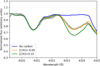 |
Fig. 1 Spectral synthesis in the CH region at 4300 Å for HD 984. |
2.2 KPIC observations of HD 984 B
We observed HD 984 on UT 2022 August 8 using KPIC. We obtained nine spectral orders in K band, ranging from approximately 1.94–2.49 pm. Similar to the observing strategy described in Wang et al. (2021b), the host star was first observed twice using the four fibers for calibration purposes with an expo- sure of 60 s. From these exposures, we measured the end-to-end throughput from the top of the atmosphere to the detector for each fiber. Based on the fiber with the best throughput (~4%, designated as the primary science fiber), the tip/tilt mirror on the fiber injection unit (FIU) was the used to offset the star from the fiber bundle and to place the companion of interest on the primary science fiber. The offset amplitude and direction were computed using the orbital prediction tool whereistheplanet3 (Wang et al. 2021a).
Two exposures were acquired for HD 984 B with an inte- gration time of 600 s each so that the read-out noise would be negligible. By taking the difference in integration time between the host star and its companion into account, we measured a companion flux corresponding to ΔK = 7.1 ± 0.3 mag, which is within 3σ of the expected ΔK = 6.13 ± 0.05 mag reported in the literature (see Tables 1 and 2). In addition to these spectra, an M giant star (HIP 95771) and a telluric standard star (HIP 115119) were also observed for calibration and wavelength solution pur- poses. Twelve exposures of 1.5 s each and five exposures of 60 s each were taken for HIP 95771 and HIP 115119, respectively. A summary of the different observations taken during the night are presented in Table 3.
Properties for HD 984 B.
Summary of the observations taken on UT 2022 August 8.
3 Data reduction
3.1 Raw data reduction
We followed the procedure described in Wang et al. (2021b) to extract spectra from the raw data. This procedure has been implemented in a public Python pipeline4 by the KPIC team. First, the thermal background from the images as well as the identified bad pixels were removed using the combined instru- ment thermal background frames. Then, the trace of each of the four science fibers in each of the nine orders was measured using the data from the telluric standard star HIP 115119. This star was mainly chosen for its spectral type (A0V) because it shows only a few stellar lines in the K band and has a similar eleva- tion (air mass) as our target HD 984. A 1D Gaussian was fitted to the cross-section of the trace in each column of each order to determine the position and standard deviation of the Gaussian line-spread function (LSF). To mitigate measurement noise and biases from telluric lines, the measurements of the position and standard deviations were smoothed by fitting a cubic spline.
For every frame, the 1D spectra were then extracted in each column of each order. To correct for the imperfect background subtraction, we additionally subtracted the residual background level in each column by measuring the median of pixels that were at least 5 pixels away from the center of any fiber. Finally, for each fiber, we used optimal extraction (Horne 1986) to sum the flux using the positions and standard deviations defined by the 1D Gaussian LSF profiles calculated from spectra of the telluric star.
Since the transmission of the telescope and instrument varies with wavelength due to the blaze function, we observed the M giant star HIP 95771 to determine the wavelength solution from the stellar and telluric spectral lines. This M 0.5III star was chosen because it has myriad narrow stellar lines in the K band and a well-known RV, making it a good target for wave- length reference. First, we modeled the wavelength solution as a spline using six nodes per order. HIP 95771 was modeled with a PHOENIX stellar spectrum (Husser et al. 2013) assum- ing a temperature of 3800 K, a surface gravity of log g = 1.5, solar metallicity, and a fixed known RV of −85.391 km s−1 taken from SIMBAD5. The telluric transmission of Earth’s atmo- sphere was modeled from a planetary spectrum generator model (Villanueva et al. 2018). To model the spectrum-dependent trans- mission, we then jointly fit for the wavelength solution, telluric parameters, and instrument and telescope transmission using the Nelder–Mead optimization (Virtanen et al. 2020). For more details on the wavelength calibration, we refer to Wang et al. (2021b).
3.2 Preliminary analysis
Our extracted spectra of HD 984 B consist of a mixture of light coming from the brown dwarf companion and stellar speckles. We therefore used a forward model for the signal from the planet fiber (Dp) via
 (2)
(2)
where T is the transmission of the optical system (i.e., atmo- sphere, telescope, and instrument), and PLSF and SLSF are the spectrum from the planet and from the star, respectively, after convolution by the instrumental LSF. αp and αs are the scaling factor for the planetary and stellar brightness, respectively, and n is the noise. Because of the high S/N per spectral channel of the stellar spectra (~300), the noise n was assumed to be negligible.
We explain next how we measured each parameter of Eq. (2). First, we measured the transmission T using a PHOENIX model mimicking the HIP 115119 spectrum assuming an effective tem- perature of 9600 K, a surface gravity of log(g) = 3.5, and solar metallicity. HIP 115119 was chosen because it is an A0V star, and thus, the created model has nearly no spectral lines in the K band. This mitigates any errors due to an imperfect stellar spectrum. Then, T was obtained by dividing the observed telluric standard star data (Dt) by the PHOENIX model of the star (Mt),
 (3)
(3)
To model the contribution of the stellar light that leaked into the planet fiber (i.e., T × SLSF), we then used the on-axis observation of the star HD 984 itself. Finally, PLSF was determined using a planetary atmospheric model, and the variables αp and αs were measured by finding the best fit to the data.
As a preliminary step, we confirmed the detection of HD 984 B by applying a modified cross-correlation analysis, as described in Ruffio et al. (2019) and Wang et al. (2021b). This technique consists of estimating the maximum likelihood value for both the planet and star flux as a function of RV shift for a given planet template. More explicitly, we searched for the max- imum likelihood between our Eq. (2) and our observed planetary data. To do this, we built a companion model and a stellar model in order to fit our data. Since the S/N of KPIC is optimized for wavelengths around 2.3 μm (i.e., where the CO has a series of strong absorption lines), we focused our analysis on three spec- tral orders, from 2.29 to 2.49 μm. These three orders are the best suited for an analysis of HD 984 B because they contain the strongest absorption lines from the companion and have few telluric absorption lines.
Our companion model was first built using a BT-Settl-CIFIST model grid (Baraffe et al. 2015). A BT-Settl planetary atmospheric model was chosen as it was the only publicly avail- able grid of models with a spectral resolution R > 35 000 and with an effective temperature Teff ~ 2800 K that includes clouds. The presence of clouds in our model might be particularly important for high-resolution spectra because clouds change the depths of molecular absorption lines (Hood et al. 2020; Mollière et al. 2020). Our planetary model was then shifted to fit for the RV. Then, the model was rotationally broadened by a pro- jected rotation rate v sin i and convolved using the instrumental LSF. Finally, the companion model was multiplied by the telluric response function T. In the last steps, we removed the continuum variations of the models and planetary data. A high-pass filter- ing was applied with an optimal median filter size of 100 pixels (~0.002 μm), as determined in Xuan et al. (2022). After scaling the companion and speckle models using different αp and αs for each order, we fit the total model to the data and searched for the maximum likelihood value.
From this modified and normalized cross-correlation between the KPIC data and the BT-Settl model, we confirmed the clear detection of HD 984 B with an S/N of ~25 (see Fig. 2). Additionally, we find that H2O and CO are detected with an S/N of 20 and 18, respectively, using single-molecule templates (built from the best parameters found from our petitRADTRANS retrievals; see Sect. 4.2). We note that while several other atomic lines are expected in the stellar atmospheres of targets with Teff = 2700 K in the K band, such as Na, Ca, Al and Fe, they only appear as a handful of single lines, which makes it hard to properly identify them with CCFs. The standard deviation of the wings of the CCF were used to estimate its noise and to normal- ize the CCF. We measured a RV of −25.8 km s−1, which is within the 1σ error bar from the expected value (−23.4 ± 5 km s−1) obtained from the orbital prediction tool whereistheplanet (based on the GRAVITY data, unpublished), by taking the RV of its host star into account and adding the barycentric correc- tion, including the effect caused by the Earth’s rotation. Finally, using the atmospheric template, we broadened the results of its autocorrelation function and found that the best fit to the CCF was approximately 15 km s−1, giving us a first estimate of the rotational velocity of HD 984 B. This result is also shown in Fig. 2, where we plot the ACF and its broadened version, both rescaled to the peak value of the CCF.
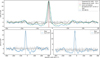 |
Fig. 2 CCFs between the KPIC data (using the three orders from 2.29 to 2.49 μm) and different models. Top panel: CCFs between the KPIC data and a BT-Settl model (see Sect. 3.2). The CCF for HD 984 B is plotted in blue, and for comparison, we add the CCF of the stellar data in gray. The autocorrelation of the planetary model is also shown in black. The standard deviation of the wings of the CCF were used to estimate its noise and to normalize the CCF. The dashed vertical gray and red lines show the expected and measured RV of the companion (−23.4 km s−1 and −25.8 km s−1, respectively). Bottom panels: CCFs showing the H2O and CO detection from the same KPIC data after using single-molecule templates. |
Priors for the HD 984 B retrieval.
4 Spectral analysis
4.1 Atmosphere retrieval
After the preliminary analysis of our data, which confirmed the presence of the planetary companion using a BT-Settl model, we repeated our analysis using a free retrieval framework based on the open-source radiative transfer code petitRADTRANS (Mollière et al. 2019). This section describes how we built our models to fit the data.
4.1.1 Opacities
Following our preliminary analysis (described in Sect. 3.2), our goal was to combine a companion model and a stellar speckle model to fit our data. Instead of using self-consistent grid mod- els, petitRADTRANS allows more flexibility to fit the data, which provides much more detailed information about the atmospheric properties. This method has been used in previous studies (e.g., Mollière et al. 2020; Xuan et al. 2022) that proved that it can retrieve the chemical abundances, vertical temperature structure, and cloud properties of exoplanets and brown dwarfs. The flex- ibility of the retrieval approaches makes them ideal for explor- ing the properties of complex objects such as brown dwarfs and exoplanets, but it can also lead to occasional unphysical results. This is why the choice of our priors and boundaries is important (see Table 4).
In order to correctly set our model up, we first used the line-by-line opacity sampling method in petitRADTRANS for the retrieval, including opacities for H2O, 12CO, 13CO, CO2, FeH, NH3, and H2S. The choice of these opacities was made based on the relatively high effective temperature of HD 984 B (2730 K) and on the selected observed wavelength range in the K band (between 2.29 and 2.49 μm). For completeness in our retrieval, we also searched for methane in the atmo- sphere of HD 984 B. We used the HITEMP CH4 line list from Hargreaves et al. (2020), which was converted into opacities for use in petitRADTRANS as explained in Xuan et al. (2022). Collision-induced absorption (CIA) opacities of H2-H2, H2-He, and H- were also accounted for in our retrieval as these species are important absorbers in the K band.
4.1.2 Temperature model
We set the vertical extent of the atmosphere of our brown dwarf using a pressure-temperature (P – T) profile between P = 10−4−102 bars and followed the P − T profile definition from Mollière et al. (2020). This definition parameterizes the vertical temperature profile of the atmosphere into three differ- ent parts: high altitudes, the photosphere (middle altitudes), and the troposphere (low altitudes), where the spatial coordinate of the temperature model is an optical depth (τ), defined via
 (4)
(4)
with δ and a being two free parameters. It should be noted that a was restricted to vary only between 1 and 2, following Robinson & Catling (2012).
For the high altitudes (between the top of the atmosphere to τ = 0.1), the atmosphere was fit with three temperature points equidistant in log(P) space, which were treated as free parameters. These three temperature points were defined such that they were colder than the highest point of the photosphere and such that they monotonically decreased in temperature with increasing altitude in order to prevent the formation of temper- ature inversions. For the photosphere (between τ = 0.1 to the radiative-convective boundary), the temperature was set accord- ing to the Eddington approximation with T0 as the internal temperature. Finally, for the troposphere (between the radiative- convective boundary to the bottom of the atmosphere), it was forced to follow the moist adiabatic temperature gradient as soon as the atmosphere was found to be Schwarzschild-unstable (Mollière et al. 2020).
4.1.3 Chemistry model
We followed the equilibrium chemistry model described in Mollière et al. (2019) to compute the abundance of each absorb- ing molecule. These abundances were defined as a function of pressure, temperature, carbon-to-oxygen number ratio (C/O) and metallicity ([Fe/H]). The temperature ranged from 500 to 4000 K, the C/O values from 0.1 to 1.6, and the [Fe/H] from −1.5 to 1.5. Since the S/N of our data is relatively high, we also stud- ied the abundance of the 13CO isotope by fitting in our retrieval the 12CO/13CO ratio (ranging from 0 to 6 in log-scale).
To account for the possibility of disequilibrium chemistry, we included a quench pressure term (Pquench) as a free parameter. This disequilibrium chemistry can arise when the atmospheric mixing timescale is shorter than the chemical reaction timescale. For atmospheric pressures P < Pquench, we therefore fixed the abundances of H2O, CO, and CH4 using the equilibrium value found at Pquench, following the results from Zahnle & Marley (2014).
4.1.4 Clouds
In our analysis, we considered both clear (i.e., without clouds) and cloudy models to compare our retrieved abundances. For the latter, we used the EddySed model from Ackerman & Marley (2001) as implemented in petitRADTRANS, where the cloud par- ticles both absorb and scatter the absorbing photon from the atmosphere. By taking the effective temperature of HD 984 B into account and comparing the results from Wakeford et al. (2017) and Gao et al. (2020) for the most likely cloud species as a function of temperature, we decided to consider three dif- ferent cloud species: Fe, MgSiO3, and Al2O3. We assumed their crystalline phases. In particular, Al2O3 appears to be the most important species of the three when we compare their conden- sation curves with different thermal profiles from the Sonora atmospheric model (Marley et al. 2021). In addition, MgSiO3 is also expected to be one of the most important cloud species for substellar objects with Teff > 950 K because its nucleation energy barriers are low and the elemental abundances of Mg, Si, and O are relatively high (Gao et al. 2020).
Three free parameters (fsed, Kzz, and σg) are needed to con- trol the mean particle size, cloud mass fraction, and particle size distribution independently (Ackerman & Marley 2001). First, by setting fsed we can retrieve the sedimentation efficiency. Then, using the vertical eddy diffusion coefficient (Kzz), we set the par- ticle size for a given fsed value. Finally, by fitting for the width of the log-normal size distribution (σg), we specified the par- ticle size distribution. Following Mollière et al. (2020), we let these parameters vary independently between 0 to 10 for fsed, 5 to 13 for log(Kzz) (with Kzz expressed in cm2 s−1), and 1.05 to 3 for σg. We also took into account as free parameters the scal- ing factor for the cloud mass fraction at the cloud base,  , for each of the cloud species used in our retrieval (i.e., Al2O3, Fe, and MgSiO3), defined such that
  refers to the mass fraction predicted for the cloud species when equilibrium condensation is assumed at the cloud base location.
4.2 Fitting with nested sampling
4.2.1 Priors
To derive the posterior distributions for HD 984 B we used the nested-sampling approach as implemented in dynesty (Speagle 2020). We chose nested sampling (over the more classi- cal Markov chain Monte Carlo, MCMC) because it is faster and can approximate the probability of the model via the Bayesian inference, which facilitates the model comparison. Specifically, we used the dynamic nested-sampling method, which allocates live points dynamically instead of using a constant number of live points, to improve the posterior density estimate. We used 500 live points to start the initial run, and we adopted the stop- ping criterion that the estimated contribution of the remaining prior volume to the total evidence be less than 1%. We also repeated our retrieval using 1000 initial live points and found that the evidence remained the same.
Similar to Mollière et al. (2020), we adopted uniform or log- uniform priors for all parameters. Table 4 presents the parameters and their priors as we used them in our retrieval. We dis- tinguished between those needed for a clear model and the additional parameters needed for a cloudy model. The Pphot quantity was used to constrain the δ parameter from Eq. (4), and it is defined as the pressure for τ = 1. Tconnect is the upper- most temperature of the photospheric layer, calculated by setting τ = 0.1 in the Eddington approximation (see Mollière et al. 2020), and it was used to constrain the T3 parameter. We addi- tionally fit the radius of HD 984 B. Using evolutionary and mass-radius models (Baraffe et al. 2003, 2008), we decided to constrain the radius between 0.5 and 2.3 RJup. We chose the pri- ors of the RV and of the v sin i parameters based on the results of our preliminary analysis (see Sect. 3.2). Finally, we also took the uncertainty in the line spread function into account (noted σs). This uncertainty is due to the difference of a factor of 1.13 in the focal lengths in the spatial and dispersion directions of the NIRSPEC spectrograph (Robichaud et al. 1998). Follow- ing Wang et al. (2021b), we let σs vary between 1.0 and 1.2 to conservatively account for any systematics.
4.2.2 Retrieval with a clear model
Using a clear model, we were able to precisely retrieve most of the companion parameters. For clarity, a corner plot pre- senting selected retrieved parameters is shown in Fig. 3. An extended corner plot can be found in the appendix (see Fig. A.1). For instance, we retrieved an RV of  and a v sin i of
  , which correspond well to our first guess from our CCF (see Fig. 2) and is comparable to the rotation rates observed for brown dwarfs with similar spectral types (Konopacky et al. 2012). We also retrieved a C/O ratio of 0.49 ± 0.01 for HD 984 B which is consistent with the solar value and is < 1σ consistent with that of its host star (due to its large error bar, 0.40 ± 0.20). Using our clear model, we were also able to detect the 13CO isotopolog in the atmosphere of HD 984 B and we measure an isotopolog 12CO/13CO ratio of
  .
.
Figure 4 shows the results of our analysis from the param- eters retrieved using nested sampling and petitRADTRANS. We plot the best-fit companion model, the speckle model, and the full model, which is the sum of the previous models. We also plot the residuals, for which no evidence of correlated noise or strong systematics was found. While we precisely retrieved some parameters with our clear model, other parameters were not well constrained (see Fig. A.1). Our retrieval failed, for exam- ple, to properly constrain the radius of HD 984 B or the quench pressure term (Pquench). This outcome can be explained by the hot temperature of HD 984 B, which makes it extremely diffi- cult to detect CH4 and therefore precludes a robust constraint on Pquench.
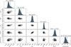 |
Fig. 3 Posterior distributions for some of the key parameters of our clear model retrieval for HD 984 B. The titles at the top of each histogram show the median and the 1σ error. |
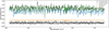 |
Fig. 4 Retrieval results normalized for HD 984 B. The KPIC data are plotted in black. The companion model retrieved using nested sampling and petitRADTRANS is plotted in blue, scaled using the retrieved αp from our fit. The companion model does not include tellurics (i.e., we show the model before it was multiplied to the telluric response function) to focus on the molecular features, but tellurics are included in our fits. The stellar model used to model the speckle contribution is plotted in orange, scaled using the retrieved αs from our fit. The full model (i.e., combination of the companion and speckle model) is shown in dashed green. The residuals between the KPIC data and our retrieved model are shown as the gray points to the bottom. The x-axis is restricted for clarity, and we focus on one order only instead of the full data range (between 2.29 and 2.49 μm). |
4.2.3 Comparison with cloudy models
After fitting a clear model, we investigated different types of cloudy models. For instance, we studied a gray cloud model that adds a constant cloud opacity to the atmosphere to examine the possibility of finding clouds at lower pressures. We also tested a variety of combinations for the cloud species using Al2O3, Fe, and MgSiO3 . For each retrieval, we measured and compared their Bayes factor (B) in order to assess the probability of each model. Table 5 summarizes the different tests showing the mod- els used, some of the retrieved parameters obtained, and the measured Bayes factor for each test compared to the clear model.
From these results, we first observe that all models are con- sistent with each other, with Bayes factor values that do not vary too much relative to the clear model. We also note that despite the high temperature of HD 984 B, Al2O3 does not have a major impact in its atmosphere, as might have been expected (see Sect. 4.1.4). This result could be due to the fact that Al2O3 has a much lower relative cloud mass than Fe and MgSiO3 (by a factor 10–20; see Wakeford et al. 2017). Given their similar Bayes factor, these results also show that clouds do not seem to play an important role in the high dispersion spectroscopy of the atmosphere of HD 984 Bin general. This result could be explained by the fact that the cloudy parameters of our retrieval mostly affect the continuum, which is ignored in the analysis of our KPIC data. We stress, however, that for the remainder of the paper, we consider the values retrieved from the EddySed (MgSiO3 + Fe, cd) model as our most likely results. This model shows the highest Bayes factor, with ln(B) = 3. 3, which corre- sponds to a ~4.3σ preference for the Trotta (2008) scale (see Fig. A.2 for the posterior distribution for our best-fit model).
Table 5 also shows that the isotopolog13 CO is detected in the atmosphere of HD 984 B in each retrieval, and the values obtained are consistent among the models, with an isotopolog 12CO/13CO ratio of  . To confirm this detection, we also tested the retrieval using a clear model without 13CO and an EddySed (MgSiO3 + Fe, cd) retrieval without 13CO models (see the bottom of Table 5). Bayes factors of ln(B) = −7. 8 and −7. 1 were measured, respectively, corresponding to a ~6.3σ and a ~6.1σ using the Trotta (2008) scale. This confirms the detection of 13CO at a significance of ~6σ sigma.
To prove that this detection is not due to our retrieval sim- ply fitting some artifacts, we also used the cross-correlation approach as an alternative detection method. By using a CCF, we expect a clear peak for the species at the companion posi- tion. However, it is important to note that in contrast to what was done for H2O and CO (see Fig. 2), we cannot simply cross-correlate our data with a 13CO template because a pure 13CO template interferes too strongly with other species (e.g., H2O and CO), which could lead to a false detection. Instead, we used the residuals between our data and our best-fit full model without taking 13CO into account. Thus, if 13CO is present in our data, it should be highlighted in these residuals. Figure 5 shows the CCF between these residuals and a 13CO template in blue. As expected, a peak appears at the exact RV shift measured for HD 984 B. This confirms the detection of 13CO. In compar- ison, we repeated the same analysis, but this time, took 13CO into account in our best-fit full model. The residuals obtained by this approach should therefore remove 13CO. From these second residuals, we indeed observe no peak (i.e., no detection) in the new CCF, plotted in red, at the companion position, as expected.
Table 5 also shows that the measured C/O ratios all match that of the host star (0.40 ± 0.20), with a C/O ratio of 0.50 ± 0.01. Similarly, the measured metallicity values are all consistent in the different models, and we infer that HD 984 B has a sub- stellar metallicity with ![Mathematical equation: $\left[ {{\rm{Fe/H}}} \right] = - 0.62_{ - 0.02}^{ + 0.02}$](/articles/aa/full_html/2024/06/aa48370-23/aa48370-23-eq48.png) . Hence, we find that the C/O ratio, the metallicity, and the 13CO ratio values do not strongly rely on the accurate inference of the tempera- ture structure and clouds (as was found in Mollière et al. 2020; Burningham et al. 2021; Zhang et al. 2021b), and that the values found for these parameters are independent of the assumptions on the clouds.
. Hence, we find that the C/O ratio, the metallicity, and the 13CO ratio values do not strongly rely on the accurate inference of the tempera- ture structure and clouds (as was found in Mollière et al. 2020; Burningham et al. 2021; Zhang et al. 2021b), and that the values found for these parameters are independent of the assumptions on the clouds.
Using the parameters retrieved from our best-fit model, we show in Fig. 6 the retrieved P – T profiles. For comparison, we also plot three cloud condensation curves (for MgSiO3, Fe, and Al2O3) and three different Sonora P – T profiles Marley et al. 2021 with properties similar to HD 984 B. These can be used to confirm where the cloud condensation curves are expected to intersect the P – T profile. As an example, the Sonora thermal profile of Teff = 2600 K and log g = 5.0 intersects the conden- sation curve of Al2O3 near 0. 04 bar, in comparison with the condensation curves of Fe and MgSiO3, which intersect at lower pressure, around 0. 007 and 0. 003 bar. Finally, we added the emission contribution function to Fig. 6 to quantify the relative importance of the emission. This emission contribution function shows that the data are sensitive to pressures ranging from a few bar up to ~10−3 bar.
Figure 6 shows that the lower atmosphere is very consistent with the Sonora thermal profile of Teff = 2600 K and log g = 5.0, while the upper atmosphere is colder and less isothermal. In the EddySed model, the cloud base is set at the intersection of the P – T profile and a given cloud condensation curve. Hence, the lack of features in the emission contribution function at this intersection shows that our high-resolution data set is largely insensitive to clouds. This is expected due to our relatively small wavelength range, 2.29–2.49 μm, and due to the high tempera- ture of HD 984 B. We also note that the clear model gives almost identical P – T shapes.
Comparison of the spectrum retrievals for HD 984 B.
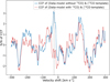 |
Fig. 5 CCFs between residuals of our best-fit full model and a 13CO template. The CCF shown in blue corresponds to the residuals between our KPIC data and our full model without taking 13CO into account. Conversely, the CCF in red corresponds to the residuals between our KPIC data and our full model while taking 13CO into account. The peak in the blue CCF (that is absent in the red CCF) at the exact RV shift measured for HD 984 B shown with a vertical gray line, confirms the presence of 13CO in our data. |
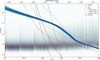 |
Fig. 6 The P – T profile from our best-fit retrieval (model MgSiO3 + Fe). The best-fit profile is shown in black, and 200 random draws from the posterior are shown in blue. The condensation curves for different cloud species (MgSiO3, Fe and Al2O3) are also plotted. In addition, we show multiple Sonora P – T profiles as dashed lines (Marley et al. 2021) with similar properties as HD 984 B. Finally, we plot the emission contribution function (in wavelength, top axis) as contours, which quantifies the relative importance of the emission in a given pressure layer to the total at a given wavelength (Mollière et al. 2019). |
5 Discussion and summary
This paper presented the observation and characterization of the hot brown dwarf HD 984 B using high-resolution spectroscopic KPIC data. Using the nested-sampling technique and petitRADTRANS we tested different forward-retrieval models using both clear and cloudy models, and we measured some of the properties of this companion. Our results are listed below.
By comparing the measured Bayes factors, we found that the different models we tested were consistent with each other. In addition, most of the measured parameters seem indepen- dent of assumptions about the presence or absence of clouds, nor do they rely on the accurate inference of the tempera- ture structure. While we used the EddySed (MgSiO3 + Fe, cd) model as our main model because it has the highest Bayes factor (with ln(B) = 3.3), we found no evidence of a cloudy atmosphere for HD 984 B, which can be explained by the fact that the clouds are probably at too high a pressure in the atmosphere of HD 984 B to have a major impact in our high-dispersion data. For instance, no cloudy features could be observed in the emission contribution pre- sented in Fig. 6, where the cloud condensation curves of MgSiO3 and Fe should have intersected with our retrieved P – T profile.
From our best-fit atmospheric model, we measure an RV of
 and a v sin i of
  for HD 984 B. We also found consistent metallicity values, with
 ![Mathematical equation: $\left[ {{\rm{Fe/H}}} \right] = - 0.62_{ - 0.02}^{ + 0.02}$](/articles/aa/full_html/2024/06/aa48370-23/aa48370-23-eq51.png) , inferring that HD 984 B has a substel- lar metallicity. This substellar metallicity seems surprising and may imply that our results are biased because the K band alone is potentially not the best band to determine the metallicity (see GRAVITY Collaboration 2020). This hypothesis, however, contradicts other results found in pre- vious papers (see, e.g., Wang et al. 2023; Xuan et al. 2024b), where the metallicity was measured to 0 2–0 3 dex on other benchmark brown dwarfs. In future work, measurements of its metallicity at other wavelengths could be used to con- firm the surprisingly low metallicity or find the source for a metallicity bias in the KPIC measurements.
, inferring that HD 984 B has a substel- lar metallicity. This substellar metallicity seems surprising and may imply that our results are biased because the K band alone is potentially not the best band to determine the metallicity (see GRAVITY Collaboration 2020). This hypothesis, however, contradicts other results found in pre- vious papers (see, e.g., Wang et al. 2023; Xuan et al. 2024b), where the metallicity was measured to 0 2–0 3 dex on other benchmark brown dwarfs. In future work, measurements of its metallicity at other wavelengths could be used to con- firm the surprisingly low metallicity or find the source for a metallicity bias in the KPIC measurements.The C/O ratio values measured for the clear and cloudy models match the value of its host star (0 40 ± 0 20). This chemical homogeneity between a companion and its host star is expected for models in which the brown dwarf com- panion formed via gravitational fragmentation in molecular clouds or massive protostellar disks (Padoan & Nordlund 2004; Stamatellos et al. 2007). In addition, the high orbital eccentricity of HD 984 B (~0.76) could contribute to the formation scenarios presented by some simulations, which suggested that brown dwarfs typically form in unstable mul- tiple systems that undergo chaotic interactions (Thies et al. 2010; Bate 2012). From our best-fit model, we measured a C/O ratio of 0.50 ± 0.01. This 0.01 error is the statistical pre- cision and might not be realistic. By comparing the results obtained from different epochs, we could assess some level of systematic error (e.g., as done in Xuan et al. 2024b). Due to the large error bar found for the C/O ratio of the host star, HD 984 B might still be enriched in C/O compared to HD 984. While unlikely, this could be explained if HD 984 B formed close to the CO ice line from material enriched in carbon (Ali-Dib et al. 2014; Schneider & Bitsch 2021).
Finally, we detected for all models the isotopolog 13CO in the atmosphere of HD 984 B. We first found a 12CO/13CO ratio of
 for the clear model, which is slightly above the carbon isotope ratio measured for the Sun (93.5 ± 3, Lyons et al. 2018). However, the 12CO/13CO ratio value measured for our best-fit cloudy model is
  which is within the 1σ error bar of the solar value and higher than the ratio of the local interstellar medium (~68, Milam et al. 2005). These results are expected for young objects (e.g., Zhang et al. 2021b), and by comparing our measured car- bon isotopolog ratio to other objects, we might constrain possible formation mechanisms. For instance, Zhang et al. (2021a) measured a 12CO/13CO ratio of ~31 for a young and wide-orbit super-Jupiter. Super-Jupiters might form via the core-accretion scenario (Pollack et al. 1996; Lambrechts & Johansen 2012), which can lead to 13CO enrichment through ice accretion. This would lower the 12CO/13CO ratio. Hence, the higher 12CO/13CO ratio value measured for HD 984 B could favor another formation scenario in which the brown dwarf is formed via gravitational collapse or disk instability. This hypothesis is corroborated by our observations of the C/O ratio.
From these results, we can infer the likely formation mech- anism of HD 984 B, namely that this hot brown dwarf probably formed via turbulent fragmentation in a molecular cloud or disk instability. This conclusion would confirm the trend of chemical homogeneity observed between brown dwarf companions (with masses ~13–70 MJup) and their host stars (e.g., Wang et al. 2022; Xuan et al. 2022, 2024a; Hsu et al. 2024).
However, our analysis revealed that not all of the parameters were properly constrained and pointed out some of the limits of this study. By only using a small wavelength range (between 2.29 and 2.49 μm), we did not fully constrain some bulk prop- erties of HD 984 B, such as some of the cloudy parameters and the radius of the companion. To better constrain the cloud prop- erties and abundances, it would be important to consider a joint analysis with available low-resolution spectroscopy data or with high-resolution spectroscopy in other spectral bands, such as the H band with the Rigorous Exoplanetary Atmosphere Charac- terization with High dispersion coronography (REACH; Kotani et al. 2020) or the High-Resolution Imaging and Spectroscopy of Exoplanets (HiRISE; Vigan et al. 2024). The addition of mid- infrared spectroscopy from the James Webb Space Telescope will also bring major insight in the coming years for our under- standing of the atmosphere of substellar companions (e.g., Carter et al. 2023; Miles et al. 2023).
Acknowledgements
J.C. and A.V. acknowledge funding from the European Research Council (ERC) under the European Union’s Horizon 2020 research and innovation programme (grant agreement No. 757561). Funding for KPIC has been provided by the California Institute of Technology, the Jet Propul- sion Laboratory, the Heising-Simons Foundation (grants #2015-129, #2017-318, #2019-1312, #2023-4598), the Simons Foundation, and the NSF under grant AST-1611623.
Appendix A Posteriors from our retrieval
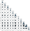 |
Fig. A.1 Extended corner plot showing the posterior distribution for our clear model retrieval for HD 984 B (see Section 4.2.2). The titles at the top of each histogram show the median and 1σ error. |
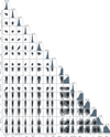 |
Fig. A.2 Extended corner plot showing the posterior distribution for our best-fit cloudy model retrieval EddySed (MgSiO3 + Fe, cd) for HD 984 B (see Section 4.2.3). The titles at the top of each histogram show the median and the 1σ error. |
References
- Ackerman, A. S., & Marley, M. S. 2001, ApJ, 556, 872 [Google Scholar]
- Ali-Dib, M., Mousis, O., Petit, J.-M., & Lunine, J. I. 2014, ApJ, 793, 9 [NASA ADS] [CrossRef] [Google Scholar]
- Alibert, Y., Mousis, O., Mordasini, C., & Benz, W. 2005, ApJ, 626, L57 [NASA ADS] [CrossRef] [Google Scholar]
- Amarsi, A. M., Nissen, P. E., & Skúladóttir, Á. 2019, A&A, 630, A104 [NASA ADS] [CrossRef] [EDP Sciences] [Google Scholar]
- Baraffe, I., Chabrier, G., Barman, T. S., Allard, F., & Hauschildt, P. H. 2003, A&A, 402, 701 [NASA ADS] [CrossRef] [EDP Sciences] [Google Scholar]
- Baraffe, I., Chabrier, G., & Barman, T. 2008, A&A, 482, 315 [NASA ADS] [CrossRef] [EDP Sciences] [Google Scholar]
- Baraffe, I., Homeier, D., Allard, F., & Chabrier, G. 2015, A&A, 577, A42 [NASA ADS] [CrossRef] [EDP Sciences] [Google Scholar]
- Bate, M. R. 2012, MNRAS, 419, 3115 [NASA ADS] [CrossRef] [Google Scholar]
- Blanco-Cuaresma, S. 2019, MNRAS, 486, 2075 [Google Scholar]
- Boro Saikia, S., Marvin, C. J., Jeffers, S. V., et al. 2018, A&A, 616, A108 [NASA ADS] [CrossRef] [EDP Sciences] [Google Scholar]
- Boss, A. P. 1997, Science, 276, 1836 [Google Scholar]
- Bowler, B. P. 2016, PASP, 128, 102001 [Google Scholar]
- Bowler, B. P., Blunt, S. C., & Nielsen, E. L. 2020, AJ, 159, 63 [Google Scholar]
- Bowler, B. P., Tran, Q. H., Zhang, Z., et al. 2023, AJ, 165, 164 [NASA ADS] [CrossRef] [Google Scholar]
- Brogi, M., & Line, M. R. 2019, AJ, 157, 114 [Google Scholar]
- Bryan, M. L., Bowler, B. P., Knutson, H. A., et al. 2016, ApJ, 827, 100 [Google Scholar]
- Bryan, M. L., Benneke, B., Knutson, H. A., Batygin, K., & Bowler, B. P. 2018, Nat. Astron., 2, 138 [Google Scholar]
- Burningham, B., Faherty, J. K., Gonzales, E. C., et al. 2021, MNRAS, 506, 1944 [NASA ADS] [CrossRef] [Google Scholar]
- Carter, A. L., Hinkley, S., Kammerer, J., et al. 2023, ApJ, 951, L20 [NASA ADS] [CrossRef] [Google Scholar]
- Casagrande, L., & VandenBerg, D. A. 2018, MNRAS, 475, 5023 [Google Scholar]
- Casagrande, L., Schönrich, R., Asplund, M., et al. 2011, A&A, 530, A138 [NASA ADS] [CrossRef] [EDP Sciences] [Google Scholar]
- Casagrande, L., Lin, J., Rains, A. D., et al. 2021, MNRAS, 507, 2684 [NASA ADS] [CrossRef] [Google Scholar]
- Chachan, Y., Knutson, H. A., Lothringer, J., & Blake, G. A. 2023, ApJ, 943, 112 [NASA ADS] [CrossRef] [Google Scholar]
- Cridland, A. J., van Dishoeck, E. F., Alessi, M., & Pudritz, R. E. 2020, A&A, 642, A229 [NASA ADS] [CrossRef] [EDP Sciences] [Google Scholar]
- Currie, T., Biller, B., Lagrange, A., et al. 2023, ASP Conf. Ser., 534, 799 [NASA ADS] [Google Scholar]
- Cutri, R. M., Skrutskie, M. F., van Dyk, S., et al. 2003, VizieR Online Data Catalog: II/246 [Google Scholar]
- Delorme, J.-R., Jovanovic, N., Echeverri, D., et al. 2021, J. Astron. Telesc. Instrum Syst., 7, 035006 [NASA ADS] [CrossRef] [Google Scholar]
- Do Ó. C. R., O’Neil, K. K., Konopacky, Q. M., et al. 2023, AJ, 166, 48 [CrossRef] [Google Scholar]
- D’Orazi, V., Oliva, E., Bragaglia, A., et al. 2020, A&A, 633, A38 [NASA ADS] [CrossRef] [EDP Sciences] [Google Scholar]
- Franson, K., Bowler, B. P., Brandt, T. D., et al. 2022, AJ, 163, 50 [NASA ADS] [CrossRef] [Google Scholar]
- Gaia Collaboration (Brown, A. G. A., et al.) 2021, A&A, 650, C3 [EDP Sciences] [Google Scholar]
- Gao, P., Thorngren, D. P., Lee, E. K. H., et al. 2020, Nat. Astron., 4, 951 [NASA ADS] [CrossRef] [Google Scholar]
- GRAVITY Collaboration (Nowak, M., et al.) 2020, A&A, 633, A110 [NASA ADS] [CrossRef] [EDP Sciences] [Google Scholar]
- Hargreaves, R. J., Gordon, I. E., Rey, M., et al. 2020, ApJS, 247, 55 [NASA ADS] [CrossRef] [Google Scholar]
- Heiter, U., Lind, K., Bergemann, M., et al. 2021, A&A, 645, A106 [EDP Sciences] [Google Scholar]
- Høg, E., Fabricius, C., Makarov, V. V., et al. 2000, A&A, 355, L27 [Google Scholar]
- Hood, C. E., Fortney, J. J., Line, M. R., et al. 2020, AJ, 160, 198 [NASA ADS] [CrossRef] [Google Scholar]
- Horne, K. 1986, PASP, 98, 609 [Google Scholar]
- Houk, N., & Swift, C. 1999, Michigan Spectral Survey, 5 [Google Scholar]
- Hsu, C.-C. H., Wang, J., & Xuan, J. 2024, AAS/Division for Extreme Solar Systems Abstracts, submitted [Google Scholar]
- Husser, T. O., Wende-von Berg, S., Dreizler, S., et al. 2013, A&A, 553, A6 [NASA ADS] [CrossRef] [EDP Sciences] [Google Scholar]
- Johnson-Groh, M., Marois, C., De Rosa, R. J., et al. 2017, AJ, 153, 190 [NASA ADS] [CrossRef] [Google Scholar]
- Kaufer, A., Stahl, O., Tubbesing, S., et al. 1999, The Messenger, 95, 8 [Google Scholar]
- Kirby, E. N., Guhathakurta, P., Bolte, M., Sneden, C., & Geha, M. C. 2009, ApJ, 705, 328 [NASA ADS] [CrossRef] [Google Scholar]
- Konopacky, Q. M., Ghez, A. M., Fabrycky, D. C., et al. 2012, ApJ, 750, 79 [NASA ADS] [CrossRef] [Google Scholar]
- Konopacky, Q. M., Barman, T. S., Macintosh, B. A., & Marois, C. 2013, Science, 339, 1398 [Google Scholar]
- Kotani, T., Kawahara, H., Ishizuka, M., et al. 2020, SPIE Conf. Ser., 11448, 1144878 [NASA ADS] [Google Scholar]
- Kratter, K. M., Murray-Clay, R. A., & Youdin, A. N. 2010, ApJ, 710, 1375 [Google Scholar]
- Lambrechts, M., & Johansen, A. 2012, A&A, 544, A32 [NASA ADS] [CrossRef] [EDP Sciences] [Google Scholar]
- Landman, R., Stolker, T., Snellen, I. A. G., et al. 2024, A&A, 682, A48 [NASA ADS] [CrossRef] [EDP Sciences] [Google Scholar]
- López, R. A., Hoffman, E. B., Doppmann, G., et al. 2020, SPIE Conf. Ser., 11447, 114476B [Google Scholar]
- Lyons, J. R., Gharib-Nezhad, E., & Ayres, T. R. 2018, Nat. Commun., 9, 908 [Google Scholar]
- Marley, M. S., Saumon, D., Visscher, C., et al. 2021, ApJ, 920, 85 [NASA ADS] [CrossRef] [Google Scholar]
- Martin, E. C., Fitzgerald, M. P., McLean, I. S., et al. 2018, SPIE Conf. Ser., 10702, 107020A [NASA ADS] [Google Scholar]
- Mawet, D., Ruane, G., Xuan, W., et al. 2017, ApJ, 838, 92 [Google Scholar]
- Meshkat, T., Bonnefoy, M., Mamajek, E. E., et al. 2015, MNRAS, 453, 2378 [NASA ADS] [Google Scholar]
- Milam, S. N., Savage, C., Brewster, M. A., Ziurys, L. M., & Wyckoff, S. 2005, ApJ, 634, 1126 [Google Scholar]
- Miles, B. E., Biller, B. A., Patapis, P., et al. 2023, ApJ, 946, L6 [NASA ADS] [CrossRef] [Google Scholar]
- Mollière, P., Wardenier, J. P., van Boekel, R., et al. 2019, A&A, 627, A67 [Google Scholar]
- Mollière, P., Stolker, T., Lacour, S., et al. 2020, A&A, 640, A131 [Google Scholar]
- Nagpal, V., Blunt, S., Bowler, B. P., et al. 2023, AJ, 165, 32 [CrossRef] [Google Scholar]
- Nielsen, E. L., De Rosa, R. J., Macintosh, B., et al. 2019, AJ, 158, 13 [Google Scholar]
- Öberg, K. I., Murray-Clay, R., & Bergin, E. A. 2011, ApJ, 743, L16 [Google Scholar]
- Padoan, P., & Nordlund, Å. 2004, ApJ, 617, 559 [NASA ADS] [CrossRef] [Google Scholar]
- Piskunov, N., & Valenti, J. A. 2017, A&A, 597, A16 [NASA ADS] [CrossRef] [EDP Sciences] [Google Scholar]
- Pollack, J. B., Hubickyj, O., Bodenheimer, P., et al. 1996, Icarus, 124, 62 [NASA ADS] [CrossRef] [Google Scholar]
- Robichaud, J. L., Zellers, B., Philippon, R., McLean, I. S., & Figer, D. F. 1998, SPIE Conf. Ser., 3354, 1068 [NASA ADS] [Google Scholar]
- Robinson, T. D., & Catling, D. C. 2012, ApJ, 757, 104 [Google Scholar]
- Ruffio, J.-B., Macintosh, B., Konopacky, Q. M., et al. 2019, AJ, 158, 200 [Google Scholar]
- Schneider, A. D., & Bitsch, B. 2021, A&A, 654, A71 [Google Scholar]
- Sneden, C. A. 1973, PhD thesis, University of Texas, Austin, USA [Google Scholar]
- Snellen, I. A. G., Brandl, B. R., de Kok, R. J., et al. 2014, Nature, 509, 63 [Google Scholar]
- Speagle, J. S. 2020, MNRAS, 493, 3132 [Google Scholar]
- Stamatellos, D., Hubber, D. A., & Whitworth, A. P. 2007, MNRAS, 382, L30 [NASA ADS] [CrossRef] [Google Scholar]
- Thies, I., Kroupa, P., Goodwin, S. P., Stamatellos, D., & Whitworth, A. P. 2010, ApJ, 717, 577 [NASA ADS] [CrossRef] [Google Scholar]
- Trotta, R. 2008, Contemp. Phys., 49, 71 [Google Scholar]
- Vigan, A., Fontanive, C., Meyer, M., et al. 2021, A&A, 651, A72 [EDP Sciences] [Google Scholar]
- Vigan, A., El Morsy, M., Lopez, M., et al. 2024, A&A, 682, A16 [NASA ADS] [CrossRef] [EDP Sciences] [Google Scholar]
- Villanueva, G. L., Smith, M. D., Protopapa, S., Faggi, S., & Mandell, A. M. 2018, J. Quant. Spec. Radiat. Transf., 217, 86 [NASA ADS] [CrossRef] [Google Scholar]
- Virtanen, P., Gommers, R., Oliphant, T. E., et al. 2020, Nat. Methods, 17, 261 [Google Scholar]
- Wakeford, H. R., Visscher, C., Lewis, N. K., et al. 2017, MNRAS, 464, 4247 [NASA ADS] [CrossRef] [Google Scholar]
- Wang, J., Mawet, D., Fortney, J. J., et al. 2018, AJ, 156, 272 [Google Scholar]
- Wang, J. J., Kulikauskas, M., & Blunt, S. 2021a, Astrophysics Source Code Library [record ascl:2101.003] [Google Scholar]
- Wang, J. J., Ruffio, J.-B., Morris, E., et al. 2021b, AJ, 162, 148 [NASA ADS] [CrossRef] [Google Scholar]
- Wang, J., Kolecki, J. R., Ruffio, J.-B., et al. 2022, AJ, 163, 189 [CrossRef] [Google Scholar]
- Wang, J., Wang, J. J., Ruffio, J.-B., et al. 2023, AJ, 165, 4 [NASA ADS] [CrossRef] [Google Scholar]
- Xuan, J. W., Wang, J., Ruffio, J.-B., et al. 2022, ApJ, 937, 54 [NASA ADS] [CrossRef] [Google Scholar]
- Xuan, J., Wang, J., Ruffio, J.-B., et al. 2024a, AAS/Division for Extreme Sol. Syst. Abstracts, 56, 626.11 [Google Scholar]
- Xuan, J. W., Wang, J., Finnerty, L., et al. 2024b, ApJ, 962, 10 [NASA ADS] [CrossRef] [Google Scholar]
- Zahnle, K. J., & Marley, M. S. 2014, ApJ, 797, 41 [CrossRef] [Google Scholar]
- Zhang, Y., Snellen, I. A. G., Bohn, A. J., et al. 2021a, Nature, 595, 370 [NASA ADS] [CrossRef] [Google Scholar]
- Zhang, Y., Snellen, I. A. G., & Mollière, P. 2021b, A&A, 656, A76 [NASA ADS] [CrossRef] [EDP Sciences] [Google Scholar]
- Zuckerman, B., Rhee, J. H., Song, I., & Bessell, M. S. 2011, ApJ, 732, 61 [Google Scholar]
- Zúñiga-Fernández, S., Bayo, A., Elliott, P., et al. 2021, A&A, 645, A30 [NASA ADS] [CrossRef] [EDP Sciences] [Google Scholar]
Programs: 072.A-9006(A), 077.C-0573(A).
All Tables
All Figures
|
Fig. 1 Spectral synthesis in the CH region at 4300 Å for HD 984. |
| In the text | |
|
Fig. 2 CCFs between the KPIC data (using the three orders from 2.29 to 2.49 μm) and different models. Top panel: CCFs between the KPIC data and a BT-Settl model (see Sect. 3.2). The CCF for HD 984 B is plotted in blue, and for comparison, we add the CCF of the stellar data in gray. The autocorrelation of the planetary model is also shown in black. The standard deviation of the wings of the CCF were used to estimate its noise and to normalize the CCF. The dashed vertical gray and red lines show the expected and measured RV of the companion (−23.4 km s−1 and −25.8 km s−1, respectively). Bottom panels: CCFs showing the H2O and CO detection from the same KPIC data after using single-molecule templates. |
| In the text | |
|
Fig. 3 Posterior distributions for some of the key parameters of our clear model retrieval for HD 984 B. The titles at the top of each histogram show the median and the 1σ error. |
| In the text | |
|
Fig. 4 Retrieval results normalized for HD 984 B. The KPIC data are plotted in black. The companion model retrieved using nested sampling and petitRADTRANS is plotted in blue, scaled using the retrieved αp from our fit. The companion model does not include tellurics (i.e., we show the model before it was multiplied to the telluric response function) to focus on the molecular features, but tellurics are included in our fits. The stellar model used to model the speckle contribution is plotted in orange, scaled using the retrieved αs from our fit. The full model (i.e., combination of the companion and speckle model) is shown in dashed green. The residuals between the KPIC data and our retrieved model are shown as the gray points to the bottom. The x-axis is restricted for clarity, and we focus on one order only instead of the full data range (between 2.29 and 2.49 μm). |
| In the text | |
|
Fig. 5 CCFs between residuals of our best-fit full model and a 13CO template. The CCF shown in blue corresponds to the residuals between our KPIC data and our full model without taking 13CO into account. Conversely, the CCF in red corresponds to the residuals between our KPIC data and our full model while taking 13CO into account. The peak in the blue CCF (that is absent in the red CCF) at the exact RV shift measured for HD 984 B shown with a vertical gray line, confirms the presence of 13CO in our data. |
| In the text | |
|
Fig. 6 The P – T profile from our best-fit retrieval (model MgSiO3 + Fe). The best-fit profile is shown in black, and 200 random draws from the posterior are shown in blue. The condensation curves for different cloud species (MgSiO3, Fe and Al2O3) are also plotted. In addition, we show multiple Sonora P – T profiles as dashed lines (Marley et al. 2021) with similar properties as HD 984 B. Finally, we plot the emission contribution function (in wavelength, top axis) as contours, which quantifies the relative importance of the emission in a given pressure layer to the total at a given wavelength (Mollière et al. 2019). |
| In the text | |
|
Fig. A.1 Extended corner plot showing the posterior distribution for our clear model retrieval for HD 984 B (see Section 4.2.2). The titles at the top of each histogram show the median and 1σ error. |
| In the text | |
|
Fig. A.2 Extended corner plot showing the posterior distribution for our best-fit cloudy model retrieval EddySed (MgSiO3 + Fe, cd) for HD 984 B (see Section 4.2.3). The titles at the top of each histogram show the median and the 1σ error. |
| In the text | |
Current usage metrics show cumulative count of Article Views (full-text article views including HTML views, PDF and ePub downloads, according to the available data) and Abstracts Views on Vision4Press platform.
Data correspond to usage on the plateform after 2015. The current usage metrics is available 48-96 hours after online publication and is updated daily on week days.
Initial download of the metrics may take a while.