| Issue |
A&A
Volume 688, August 2024
|
|
|---|---|---|
| Article Number | A219 | |
| Number of page(s) | 18 | |
| Section | Cosmology (including clusters of galaxies) | |
| DOI | https://doi.org/10.1051/0004-6361/202348411 | |
| Published online | 26 August 2024 | |
Evolution of X-ray galaxy cluster properties in a representative sample (EXCPReS)
Optimal binning for temperature profile extraction
1
Université Paris-Saclay, Université Paris Cité, CEA, CNRS, AIM, 91191 Gif-sur-Yvette, France
e-mail: gabriel.pratt@cea.fr
2
IRAP, CNRS, Université de Toulouse, CNES, UT3-UPS, Toulouse, France
Received:
27
October
2023
Accepted:
26
April
2024
We present XMM-Newton observations of a representative X-ray selected sample of 31 galaxy clusters at moderate redshift (0.4 < z < 0.6), spanning the mass range 1014 < M500 < 1015 M⊙. This sample, EXCPReS (Evolution of X-ray galaxy Cluster Properties in a Representative Sample), is used to test and validate a new method to produce optimally-binned cluster X-ray temperature profiles. The method uses a dynamic programming algorithm, based on partitioning of the soft-band X-ray surface brightness profile, to obtain a binning scheme that optimally fulfils a given signal-to-noise threshold criterion out to large radius. From the resulting optimally-binned EXCPReS temperature profiles, and combining with those from the local REXCESS sample, we provide a generic scaling relation between the relative error on the temperature and the [0.3–2] keV surface brightness signal-to-noise ratio, and its dependence on temperature and redshift. We derive an average scaled 3D temperature profile for the sample. Comparing to the average scaled 3D temperature profiles from REXCESS, we find no evidence for evolution of the average profile shape within the redshift range that we probe.
Key words: galaxies: clusters: general / galaxies: clusters: intracluster medium / X-rays: galaxies / X-rays: galaxies: clusters
© The Authors 2024
 Open Access article, published by EDP Sciences, under the terms of the Creative Commons Attribution License (https://creativecommons.org/licenses/by/4.0), which permits unrestricted use, distribution, and reproduction in any medium, provided the original work is properly cited.
This article is published in open access under the Subscribe to Open model. Subscribe to A&A to support open access publication.
1. Introduction
Galaxy clusters form through the gravitational collapse of the dominant dark matter component, with the gas of the intra-cluster medium (ICM) ‘following’ the gravitational potential as the object grows by accretion and merging. The ICM is heated to X-ray emitting temperatures by shocks and compression during this hierarchical assembly process under gravity. Feedback from active galactic nuclei, supernovae, and gas cooling further modify the properties of the ICM over cosmic time (Kravtsov & Borgani 2012; Vogelsberger et al. 2014; Schaye et al. 2015, 2023).
In this context, spatially resolved measurements of the thermodynamic properties of the ICM contain crucial information on the physics governing the formation and evolution of groups and clusters. Radial profiles of gas density, ne, and temperature, kT, have become fundamental tools for measurement of key quantities such as pressure, P, entropy, K, and hydrostatic mass, and for making comparisons with predictions from numerical simulations (see, e.g. Lovisari et al. 2022; Kay & Pratt 2022, for recent reviews). However, while the gas density is simple to obtain from X-ray imaging, determination of a radial temperature profile requires an annular binning scheme that yields sufficient signal to build and model the spectrum. The problem is compounded by the density-squared dependence of the X-ray emission, a typical cluster emissivity profile that steepens dramatically with radius, and by the drop in the signal-to-noise (S/N) at lower masses and higher redshifts.
The radial temperature profiles of local (z ≲ 0.3) clusters and groups are now well characterised (Markevitch 1998; De Grandi & Molendi 2002; Vikhlinin et al. 2005, 2006; Pratt et al. 2007; Baldi et al. 2007; Leccardi & Molendi 2008; Sun et al. 2009; Arnaud et al. 2010; Lovisari et al. 2015). The temperature declines gradually towards the outer regions from a peak at R ∼ 0.2 R500. In the inner regions, non-cool core systems are typically approximately isothermal at the peak temperature, while cool core systems exhibit a characteristic smooth drop to 1/2 − 1/3 of the peak temperature value. In particular, Vikhlinin et al. (2006) and Sun et al. (2009) showed the remarkable similarity and tight scaling with mass in relaxed systems. The Representative XMM-Newton Cluster Structure Survey (REXCESS), a representative sample of X-ray selected clusters, has provided the mean pressure profile, its dispersion, and the mass scaling (Arnaud et al. 2010) that is used in all matched multi-filter Sunyaev-Zeldovich effect (SZE) survey detection algorithms (e.g. Melin et al. 2006). It has also yielded strong constraints on the radial and mass dependence of the entropy distribution (Pratt et al. 2010).
Until recently however, individual radial temperature profiles were rarely available beyond z > 0.3 (however, see e.g. Kotov & Vikhlinin 2005; Baldi et al. 2012; Mantz et al. 2016 for pioneering studies). While the advent of SZE surveys by ACT (Hasselfield et al. 2013), SPT (Bleem et al. 2015) and Planck (Planck Collaboration XXVII 2016), has transformed the quest for high-z systems, X-ray follow-up deep enough to measure annular temperature profiles of these new z > 0.3 SZE-discovered clusters has concentrated on the highest-mass objects. Being X-ray bright, they are the ‘easiest’ systems to observe, leading to good a precision on the radial temperature distribution (see e.g. Bartalucci et al. 2017, 2019, where the individual thermodynamic profiles of systems up to z ∼ 1 are measured). Results from stacking (e.g. McDonald et al. 2014) can yield the average behaviour, but do not offer insights into the intrinsic scatter in the profiles.
In this paper we introduce the Evolution of X-ray galaxy Cluster Properties in a Representative Sample (EXCPReS). Consisting of 31 X-ray-selected clusters in the redshift range 0.4 < z < 0.6 and the mass range 0.1 − 1.3 × 10¹⁵ M⊙, EXCPReS was designed to be a moderate-redshift analogue of REXCESS. We use EXCPReS to test and validate a novel method to optimally bin X-ray data to reconstruct the 3D temperature distribution of the ICM. In the following, we present the EXCPReS sample, the XMM-Newton observations and data analysis. We describe our method for binning of the surface brightness profiles to derive optimal temperature profiles. The method is applied to the EXCPReS sample, and the resulting profiles, and their dispersion, are compared to those of the local REXCESS sample. Throughout this paper we assume a flat ΛCDM model with H0 = 70 km s−1 Mpc−1, Ωm = 0.3 and ΩΛ = 0.7. Uncertainties are quoted at the 68% confidence level. The variables M500 and R500 are the total mass within R500 and radius corresponding to a total density contrast of Δ = 500 ρc(z), where ρc(z) is the critical density of the universe at the cluster redshift.
2. The sample
Our aim is to obtain spatially-resolved temperature measurements at moderate redshift across the full cluster mass range (i.e. M500 ≳ 1014 M⊙). As SZE-selected clusters typically probe higher masses (see Fig. 1), we chose to focus instead on X-ray selected clusters at a median redshift of z = 0.5. A logical local reference in this case is the REXCESS sample (Böhringer et al. 2007), which covers a similar mass range, but at lower redshifts (0.055 < z < 0.183). The chosen median redshift of EXCPReS is the highest z for which we can define a complete sample covering the whole cluster mass range of the various ROSAT surveys. Indeed, clusters below ∼1014 M⊙ have such low luminosities that at z ≳ 0.6 they begin to fall rapidly below the detection limits of these surveys.
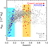 |
Fig. 1. Distribution in the M − z plane of the EXCPReS sample (red points). The local X-ray-selected REXCESS sample (Böhringer et al. 2007) is shown with blue points. Shown for comparison are confirmed clusters from major SZE surveys from which individual spatially resolved temperature profiles are measurable: Filled circles: Planck clusters (Planck Collaboration VIII 2011; Planck Collaboration XXIX 2014; Planck Collaboration XXVII 2016). Crosses: SPT (Bleem et al. 2015). Plus symbols: ACT (Hasselfield et al. 2013). |
2.1. Parent MCXC sample
Our sample is drawn from the Meta Catalogue of X-ray detected Clusters of galaxies (MCXC; Piffaretti et al. 2011). MCXC is based on the Einstein Medium Sensitivity Survey (EMSS Gioia et al. 1990; Henry 2004) and on the ROSAT All-Sky and Serendipitous surveys. We used the MCXC-II, which includes updated redshifts and ∼500 additional clusters (Sadibekova et al. 2024). Redshift revision was based on comparison of the redshifts from the NED and Simbad data bases, and cross-matching with cluster catalogues extracted from large optical surveys, in particular the SDSS (e.g. Wen & Han 2015; Rykoff et al. 2016).
The distribution in the L500–z plane of the 134 MCXC-II clusters with 0.4 < z < 0.6 is shown in Fig. 2. Different flux levels are indicated by dotted lines. These trace the [0.1–2.4] keV band flux, taking into account the Kz correction for a typical gas temperature of 5 keV. The five levels are separated by 2 dex, from 1.25 × 10⁻¹³ up to 4 × 10⁻¹² ergs s−1 cm2. Surveys are distinguished by different symbols and colours. For clusters appearing in several catalogues (i.e. detected in different surveys), we only indicate the input catalogue used to compute the luminosity, following the MCXC-II hierarchy described in Sadibekova et al. (2024).
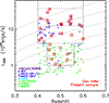 |
Fig. 2. Distribution of the MCXC clusters in the z–L500 plane (Piffaretti et al. 2011). Redshift and L500, the luminosity within R500, are from the updated MCXC catalogue (Sadibekova et al. 2024). Each cluster is colour-coded according to the survey from which the luminosity is taken. Clusters with XMM-Newton observations are marked with red circles and those included in the EXCPReS sample are marked with red boxes. The dotted lines mark the [0.1–2.4] keV band flux taking into account the Kz correction for a typical gas temperature of 5 keV. Levels are separated by 2 dex, from 1.25 × 10⁻¹³ up to 4 × 10⁻¹² ergs s−1 cm−2. |
The sub-samples of clusters from the ROSAT All-Sky survey (RASS) and the Serendipitous surveys appear quasi disjoined in the redshift range under consideration. There are 43 RASS clusters above a luminosity of 4 × 1044 ergs s−1 (flux above ≃10−12 ergs s−1 cm2), from the NORAS (Böhringer et al. 2000), REFLEX (Böhringer et al. 2004) and/or MACS catalogues. Following the MCXC-II nomenclature, the latter include the MACS-DR1 sample of the highest-z (z > 0.5) clusters (Ebeling et al. 2007), the DR2 flux-limited sample of the brightest 0.3 < z < 0.5 MACS clusters (Ebeling et al. 2010) and the deeper MACS-DR3 catalogue (Mann & Ebeling 2012, excluding overlap with DR1 and DR2)1. Only six RASS clusters lie below 4 × 1044 ergs s−1, which are clusters from the North Ecliptic Pole (NEP) deeper part of the All-sky survey (Henry et al. 2006). In contrast, all 80 clusters from ROSAT Serendipitous surveys lie at L500 < 1044 ergs s−1, with the exception of RXJ 1120.1+4318 at z = 0.6 (Romer et al. 2000). These come from the 160SD (Vikhlinin et al. 1998; Mullis et al. 2003), 400SD (Burenin et al. 2007), B-SHARC (Romer et al. 2000), S-SHARC (Burke et al. 2003), WARPS-I (Perlman et al. 2002) and WARPS-II (Horner et al. 2008) catalogues.
Finally there are five EMSS (Gioia et al. 1990; Henry 2004) clusters that were not rediscovered in the subsequent ROSAT surveys, three at luminosity below 4 × 1044 ergs s−1 and two above. The two other EMSS clusters in the redshift range are the luminous clusters MCXC J0018.5+1626 (CL0016+16 at z = 0.55) and MCXC J0454.1–0300 (z = 0.54), rediscovered in the MACS survey. Hereafter, the high-LX and low-LX subsamples include clusters above and below a luminosity of 4 × 1044 ergs s−1, respectively.
2.2. EXCPReS sample
We searched for XMM-Newton observations, with pointing position within 5′ of the cluster centre, available by September 2021 in the ESA archive2. The observed clusters are marked with red circles in Fig. 2 and those selected to form the EXCPReS sample are marked with red boxes.
The core of the EXCPReS sample is the XMM-Newton Large-Programme follow-up of EMSS, NORAS, REFLEX, B-SHARC, S-SHARC, 160SD and WARPS-I samples (programme ID #030258 with re-observation of flared observations in ID #040275 and #050243, combined with previous archival data). It was designed to study evolution from comparison with REXCESS data, similarly constructing a representative sample of clusters centered at a median redshift of z = 0.5 with homogenous coverage of the luminosity space (Arnaud 2008). The redshift excursion below L500 ∼ 4 × 1044 ergs s−1 was set to 0.45 < z < 0.55 and increased to 0.4 < z < 0.6 to include all the rare high z massive clusters known at that time. Additional observations essentially extend the high luminosity coverage, mostly thanks to the publication of MACS clusters and corresponding follow-up.
The high-LX subsample has good XMM-Newton follow-up coverage. The EMSS and REFLEX/NORAS clusters have all been observed with deep XMM-Newton pointings (nine clusters), as well as the only cluster from a ROSAT serendipitous survey (a B-SHARC object). The XMM-Newton follow-up of the MACS clusters depends on the sub-catalogues. The XMM-Newton follow-up of the MACS-DR1 and MACS-DR2 clusters is nearly complete, with twelve clusters observed. Only one MACS-DR1 cluster (MCXC J0025.4–1222 at z = 0.584) and three DR2 clusters (MACS J0152.5–2852, MACS J0159.8–0849, MACS J0358.8–2955) are lacking observations. In contrast, only three of the seventeen DR3 clusters have been observed. We decided to discard these three observations and to include the remaining 22 clusters observed by XMM-Newton. In this way, above a luminosity of 4 × 1044 ergs s−1, our sample constitutes a nearly complete follow-up, with a completion factor of 22/26 or 85%, of cluster catalogues (EMSS, NORAS/REFLEX, MACS-DR1/DR2 and B-SHARC), with a well defined selection function.
The XMM-Newton follow-up at lower luminosity is more sparse. Beyond the objects of the LP observations mentioned above, no archival observations are deep enough to allow anything but a global temperature measurement to be obtained. This is discussed in more detail in Appendix A. The final selection at low luminosity includes nine clusters in the 0.44 < z < 0.56 redshift range with L500 > 1044 ergs s−1. In this redshift range, four objects with archival XMM-Newton data are not included: one is actually a point source, and three are SHARC clusters with insufficiently deep observations.
The final EXCPReS sample comprises 31 clusters in three boxes in the L500–z plane (see Fig. 2), centred at a redshift of z = 0.5, with an approximately equal number of clusters in three equal logarithmically spaced luminosity bins. There are nine clusters in the low-luminosity bin 1044 < L500 < 4 × 1044 ergs s−1, nine clusters at intermediate luminosity, 4 × 1044 < L500 < 12 × 1044 ergs s−1, and thirteen in the high luminosity bin, 12 × 1044 < L500 < 36 × 1044 ergs s−1.
3. XMM-Newton observations and data processing
3.1. Data preparation
All data sets were retrieved and reprocessed with the XMM-Newton Science Analysis Software, using the methods described extensively in for instance Bartalucci et al. (2017). In brief, the events list were (i) cleaned for solar flare contamination (Pratt & Arnaud 2003); (ii) filtered with PATTERN-selected (0–12 for EMOS and 0–4 for EPN); (iii) corrected for vignetting (by attributing a vignetting weight function to each event, see Arnaud et al. 2001; iv) point source subtracted (after detection in the [0.3–2] keV and [2–5] keV co-added EMOS+EPN image using the SAS task +ewavedetect+, tuned to a detection threshold of 5σ and double-checked visually). All clusters have effective observation from the three XMM-Newton cameras, except MS1621.5+2640 whose PN data had to be discarded due to a high rate of contamination by solar flares. Table 1 lists the observation details for the sample. Exposure times are the sum of EMOS (EMOS1 and EMOS2) and the EPN effective exposure time (i.e. after flare cleaning).
EXCPReS sample and XMM-Newton observations.
The (solar) particle plus instrumental background templates used in later spatial and spectral analysis were obtained by stacking Filter Wheel Closed (FWC) observations for each camera. The same cleaning, PATTERN selection and vignetting correction steps were applied to the FWC events lists. The FWC files were finally cast to match the astrometry of each cluster observation and renormalised to the quiescent count rate in the [10–12] and [12–14] keV bands for EMOS and EPN, respectively.
3.2. Imagery and spectral analysis
Images and surface brightness (SX) profiles were extracted in the [0.3 − 2.0] keV band in order to maximise the S/N. The SX data points were defined in fixed circular radial bins of  width, hence assuming spherical symmetry.
Spectral analysis followed that described extensively in Pratt et al. (2010) and Bartalucci et al. (2017). Spectra were extracted in various regions of interest from the weighted events lists. The instrumental background was subtracted using the FWC spectrum from the same region in detector coordinates, normalised in the high-energy band. The cosmic X-ray background was obtained from modelling an FWC-subtracted region external to the cluster emission, normalised in the high energy band (accounting for chip gaps, missing pixels, etc)3. The model used was the sum of an unabsorbed thermal model (local bubble) added to the absorbed sum of a thermal (Galactic halo) and power law (CXB) models. It is considered constant across the cluster area and geometrically scaled in normalisation to each annulus in the modelling step. The cluster spectra were fitted with an absorbed redshifted thermal model (mekal under XSPEC), together with the CXB model above, scaled to the area of the extraction region. Fits were undertaken in the [0.3 − 10] keV band. The spectrum from the [0.15 − 0.75] R500 region was fitted with the nH free and the result was compared to the standard Leiden/Argentine/Bonn (LAB; Kalberla et al. 2005) 21 cm survey value. In no cases was the fitted nH significantly different from the LAB result, so this value was used.
3.3. Global cluster properties
The values for M500 and the corresponding R500 were computed iteratively from the M500–YX relation, calibrated by Arnaud et al. (2007) using HE mass estimates of local relaxed clusters. We assumed that the M500–YX relation obeys self-similar evolution. The quantity YX is defined as the product of the temperature TX measured in the [0.15–0.75] R500 region and the gas mass within R500 (Kravtsov et al. 2006). The gas masses were computed from the density profiles, derived from non-parametric deprojection of surface brightness profiles and the emissivity profile computed from the 2D temperature profile, as described in Croston et al. (2006). The temperature TX and mass M500 for each cluster and associated errors are reported in Table 2. The table also lists the total count rate in the [0.3–2.0] keV band within an aperture of R500 in radius, and the total S/N within the R500 aperture.
Physical parameters of the sample.
Figure 1 shows the distribution of the EXCPReS clusters in the z–M500 plane. It confirms that the sample covers a similar mass range to REXCESS with good mass sampling. However, EXCPReS extends to slightly higher masses. Four objects have masses M500 > 1015 M⊙, which is 20% larger than the maximum mass of the REXCESS sample, which is limited by the local Universe volume.
3.4. Images
We computed images in the [0.3–2.0] keV energy band in order to maximize the S/N. The images, for each available detector, were generated from the flare cleaned events lists, before point source subtraction, but corrected from the vignetting effect (with the SAS task +evigweight+). They have been excised individually for bad pixels and detector gaps, and then co-added. A count image was extracted from the EPN out-of-time events lists and subtracted from the EPN count image.
An effective exposure time image was obtained from the sum of individual detector exposure maps (outputs of SAS task +eexpmap+ without vignetting correction), weighted by the relative efficiency of each detector in the [0.3–2.0] keV band. The total count image is then divided by this exposure map and then corrected for surface brightness dimming with z, divided by the EPIC emissivity in the energy band, taking into account galactic absorption and EPIC instrument response. This final image is a map of the emission measure along the line of sight. It is then scaled according to the standard self-similar model (EM ∝ R500h(z)2), so that all images would be identical for a perfect self-similar model.
The gallery of images for our 31 clusters is shown in Figs. 3 and 4, ordered by decreasing mass. They are displayed with a linear scale. It can be seen that the clusters cover a wide range of luminosity and morphologies.
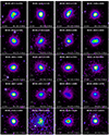 |
Fig. 3. Gallery of the XMM-Newton images, extracted in the [0.3–2] keV energy band, for the 31 clusters of the sample, ordered by decreasing mass. Image sizes are 3θ500 on a side, where θ500 is estimated from the M500–YX relation. Images are corrected for surface brightness dimming with z, divided by the emissivity in the energy band, taking into account galactic absorption and instrument response, and scaled according to the self-similar model. The colour table is the same for all clusters, so that the images would be identical if clusters obeyed self-similarity. |
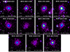 |
Fig. 4. Gallery of X-ray images for the clusters of the sample, continued. |
4. An optimal temperature profile binning method
Temperature profile binning is commonly undertaken by simply imposing a fixed bin width, or by applying some mathematical first-principle closed-form function (e.g. logarithmic binning), or by sizing the bins to obtain a given total number of counts in a given energy band. These solutions can lead to a suboptimal use of the data set by not accounting for the underlying signal and noise distributions. To exploit the spatial resolution of the instrument to its maximum, so that surface-brightness (SX) binning will yield sufficient counts per kT bin to build and model a spectrum, in the following, we describe an optimal binning algorithm based on the well-known combinatorial-optimisation algorithm ‘dynamic programming’ (Art & Mauch 2007; Cormen et al. 2009).
4.1. Problem description
The left-hand panel of Fig. 5 shows the [0.3–2] keV surface brightness profile of RX J0856.1+3756 extracted in circular  radial bins. This bin width was chosen as it is an integer multiple (3) of the XMM-Newton EPIC pn pixel size, and therefore maximises the angular resolution of the resulting SX profile in view of the mirror point spread function. The middle panel of Fig. 5 shows the resulting S/N of each SX bin as a function of bin index. The S/N is simply defined as the ratio of the SX to its statistical error, corresponding to
  in a pure Poisson regime, where N is the number of counts in a given bin. In our case the statistical uncertainties include the errors added in quadrature from subtraction of the instrumental (CLOSED) and astrophysical local backgrounds (see e.g. Bartalucci et al. 2017). The S/N profile exhibits a typical behaviour where the S/N rises sharply to a peak in the inner regions, before tapering off quasi-linearly with increasing bin index. Each individual S/N is clearly insufficient to build a spectrum, hence the need for a specific rebinning of the SX profile in order to extract the temperature profile.
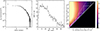 |
Fig. 5. Visual representation of the problem of binning surface-brightness (SX) bins into temperature-profile (kT) bins. Left: SX profile of RXJ0856.1+3756 in the [0.3–2] keV band, extracted in 3 |

The right-hand panel of Fig. 5 illustrates the binning problem visually. With the input SX bins labelled with increasing numbers outwards, the x-axis indicates the innermost SX bin of an output kT bin, while the y-axis indicates the outermost SX bin. The underlying colour image indicates the S/N obtained from placing the range of SX bins indicated by the axes into one single kT bin4.
A binning solution (a ‘partition’ hereafter) is then a set of adjacent kT bins that cover the entire range of SX bins. In Fig. 5, a partition is represented as a contiguous set of steps starting at (0, 0) and ending at the top-right corner. A step running from innermost SX bin a to outermost SX bin b represents an output kT bin covering input SX bins from a to b.
Figure 5 illustrates two possible partitions. The first is a partition defined by mapping two SX bin into one kT bin, which is represented as a series of two SX-bin tall steps running along the diagonal. The second is a logarithmic binning solution, which results in steps whose vertices lie along some straight line starting from the origin and having slope > 1. From such a visualisation, we would like to solve the binning problem in a data-driven way by defining a partition scheme accounting for the expected S/N level. That is, we would like the bin vertices to lie on coloured pixels having as high S/N as possible.
4.2. Definition of optimal binning
What does it mean to bin optimally? In our case, optimal binning (for temperature profile measurement) is to find a way to distribute the data signal and noise in such a way that the resulting binning scheme enables the best temperature estimation, given the characteristics of the data set in question. There are, in fact, only a finite (albeit large) number of ways of binning the input SX data into output kT bins. The exact number of solutions is 2n, where n + 1 is the number of input SX bins5. However, there are close to 300 SX bins in a typical data set of ours, so the number of possible partitions can be close to 2300 or 1030, which is intractable to compute one by one. To solve this problem we have developed an algorithm based on ‘dynamic programming’ (see e.g. Cormen et al. 2009, chap. 15), which effectively considers all possible solutions by recursively building up the optimal solution, given some algorithmic criteria.
4.3. Optimal binning algorithm
4.3.1. Fundamentals
We want our temperature profile measurements to have the best-possible distribution of S/N across the full radial range, given the characteristics of the data set in question. Generally, increasing the S/N of one kT bin implies a decrease in the S/N of an adjacent kT bin. Therefore, we will want to maximise the lowest S/N of the temperature profile annuli. Given the steep drop of cluster X-ray emission with radius, the lowest S/N temperature bin is almost always the one farthest from the centre. Conversely, in the centre, where the signal is strong, we prefer to split high-S/N kT bins into more data points having a S/N above some given requirement, rather than accumulating more signal into a single bin. We can formulate the two preferences above algorithmically as follows:
Given two partitions, A and B, of the same SX-bin range into disjoint kT bins (a.k.a. subsets):
-
The partition whose lowest subset-S/N is higher is preferable. When making this comparison, we cap subset S/Ns at the nominal requirement, thus treating all subsets with S/N above the requirement as equal.
-
If the lowest subset S/N of partitions A and B are identical, the partition whose second-lowest subset-S/N is higher is preferable.
-
This process is continued.
-
If all kT bins of partition A have (capped) S/N matching kT bins in partition B, but B has more kT bins, then B is desirable.
This selection algorithm allows us to systematically decide between any two ways of partitioning a given SX range of n bins. With the technique of dynamic programming, the optimal binning solution for the full SX-bin range (denoted OP below) is built up recursively from the union of optimal binning solutions for shorter SX-bin ranges, applying the selection algorithm at every step. If the kT-bin boundaries defined by the optimal binning algorithm are denoted a, b, c... = 0, 1, 2,...i, the algorithm is described as follows:
-
We start by considering the trivial one-SX-bin subranges [0, 0], [1, 1], [2, 2], .... The only possible (and therefore optimal), binning solution is to have one kT bin containing one SX bin: OP[a, a]=[a, a].
-
Then, we solve for two-SX-bin subranges [0, 1], [1, 2], [2, 3], .... The two possible solutions are one kT bin containing two SX bins, [a, a + 1], or two kT bins of one SX bin each, [a, a]∪[a + 1, a + 1]. We use the selection algorithm described above to decide.
-
We then solve for three-SX-bin subranges [a, a + 2] as the union of ‘optimal solutions’ for one-SX-bin and two-SX-bin subranges that we obtained above: [a, a]∪OP[a + 1, a + 2] versus OP[a, a + 1]∪[a + 2, a + 2] versus [a, a + 2]. Again, we use the selection algorithm to decide. We note that it suffices to consider only unions of two optimal partitions, OP[a, i]∪OP[i + 1, a + 2] for all possible i, and the single partition [a, a + 2] spanning the subrange in consideration. That is to say, we do not need to consider the solution [a, a]∪[a + 1, a + 1]∪[a + 2, a + 2] because it is either equivalent to [a, a]∪OP[a + 1, a + 2] and to OP[a, a + 1]∪[a + 2, a + 2], or it is not an optimal solution.
-
We then solve for four-SX-bin subranges [a, a + 3] similarly, by comparing unions of two optimal partitions, OP[a, i]∪OP[i + 1, a + 3] for all three possible i, and the single partition [a, a + 3]. Again, unions of more than two optimal partitions need not be considered explicitly, as they are either equivalent to some union of two optimal partitions, or are suboptimal.
-
We repeat the previous step to solve for all five-SX-bin subranges, then six-SX-bin, ..., until the n-SX-bin subrange, at which point we have the optimal binning of the full SX-bin range.
A key characteristic of our selection algorithm is that for Partition [a, b]∪Partition [b + 1, c] to be OP[a, c], the two child partitions themselves must be optimal as well6. This ‘optimal substructure’ is what makes dynamic programming applicable to our problem. As seen in the steps above, the recursive build-up of the final solution with dynamic programming involves computing the optimal solution for each subrange only once. These subranges are each present in an exponential number of partitions. Thus, in effect, we are breaking apart the 2(n − 1) possible partitions of an input of length n and grouping them into n(n + 1)/2 subranges, transforming the problem from enumerating and comparing an exponential number of partitions to solving for a polynomial number of subranges. It is therefore possible to cover all 2(n − 1) possible solutions in polynomial time.
The left-hand panel of Fig. 6 shows this algorithm in action, solving the binning problem in a data-driven manner for the SX profile of RXJ0856.1+3756 from Fig. 5. In this particular case, the optimal solution requires that the innermost kT bin be larger than some outer ones; a traditional approach such as logarithmic binning is not able to produce such a solution.
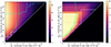 |
Fig. 6. Example binning solutions. Left: Initial binning solution for the galaxy cluster RXJ0856.1+3756 (solid white steps) from the algorithm specified in Sect. 4.3. The solid green curve delineates a 30σ S/N requirement. It shows that indefinitely adding more input SX bins to an output kT bin is suboptimal. The cyan steps represent |


It is informative to consider the roles that the partition-selection criteria play:
-
At the strong-signal end, the algorithm produces multiple data points by splitting kT bins having S/N above a given threshold. In the left hand panel of Fig. 6, it keeps these data points above, but close to, the line marking the threshold requirement.
-
At the weak-signal end, if our sole criterion were high S/N without splitting kT bins at the strong-signal end, we would always end up with one single kT bin containing all data. This is obviously not helpful in constructing a temperature profile.
-
Finally, if we split kT bins having S/N above the threshold at the strong-signal end without simultaneously imposing a S/N maximisation criterion at the weak-signal end, we would end up with the largest-radius kT bin having very low S/N, typically unusable as a temperature-profile data point. This is undesirable because this farthest bin is usually also the widest in a galaxy-cluster X-ray data set; discarding it would mean throwing away a large amount of expensive observational data.
4.3.2. A galaxy-cluster specific amendment
While our algorithm is as generic as possible, it is not specific to typical galaxy cluster X-ray data sets. This means that it still produces suboptimal output, typically yielding outermost kT bins that are too wide. It therefore requires some fine tuning to account for the characteristics of galaxy-cluster X-ray data.
The S/N pattern shown in the centre panel of Fig. 5 is very typical of X-ray observations of galaxy clusters. The S/N decrease with increasing radius is such that when starting from a particular innermost bin bin, it becomes counterproductive to include more SX bins beyond some radius bout. In the example shown in the left hand panel of Fig. 6, the 30σ contour line reaches a maximum at bin = 23, along with a corresponding bout ≈ 48. In other words, the S/N of a kT bin does not increase monotonically with the bin width. Yet the algorithm deciding between two partitions of the same SX bin range is agnostic to this peculiar property of galaxy-cluster X-ray data, resulting in the very wide outermost kT bin in the left hand panel of Fig. 6, whose S/N is not as high as it might be.
We thus need to augment the algorithm to prevent it from choosing partitions containing such suboptimal kT bins. In practice, this is achieved by modifying the S/N landscape shown in colour in the left hand panel of Fig. 6 to discourage the algorithm from choosing kT bins that are too wide, that is, those containing extraneous SX bin(s), the inclusion of which lowers the kT-bin S/N, as described in the last paragraph. Because the lowest S/N SX bins are always at large radii, the algorithm will expand the outermost kT bin inwards as much as possible – sometimes too much – to maximize its S/N in the absence of such S/N landscape modification. Instead, the optimal point to stop expanding inwards can be found by observing that if ‘for a given bin, there is a bout beyond which it is counterproductive to include more SX bins’, then the corollary is ‘for a given bout, there is an optimal bin beyond which it is not a good use of the overall data to include more SX bins, despite yielding higher S/N for the kT bin in consideration’.
In the following, we will call this optimal innermost SX bin to include  . In practice, we first obtain the optimal outermost SX bin to include by finding where the S/N reaches its maximum in each bin column, as illustrated by the cyan steps in the left hand panel of Fig. 6. This curve also gives us
  as a function of bout by the corollary above. To prevent the algorithm from moving further inwards, we therefore feed into the algorithm a modified copy of the S/N data, in which the values at
  are capped to the value at
  . This modified S/N landscape is shown in colour in the right hand panel of Fig. 6. Now, the algorithm stops moving further inwards when it reaches
  , and the resulting partitioning scheme (solid white steps) becomes optimal.
4.3.3. Algorithm variations
In practice, there are sometimes extra constraints to consider. We encode such constraints as additional modifications to the input S/N landscape, allowing us to run the optimal binning algorithm without change. For example, downstream data processing may require wider kT bins than the input single SX bins, which translates to the requirement of a minimum input SX-bin count Nin, min per output kT bin. We can implement this by zeroing the S/N values at pixels where bout − bin < Ninput, min (i.e. those closest to the diagonal). Alternatively, we may want kT bins at least as wide as those one would obtain from logarithmic binning. We can satisfy this constraint by zeroing S/N values where the ratio bout/bin is less than the desired logarithmic binning factor. We can also similarly impose a minimum S/N per output kT bin by zeroing unacceptable pixels in the input S/N landscape. The left hand panel of Figure 7 demonstrates how the algorithm operates when given a number of such constraints.
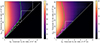 |
Fig. 7. Two algorithm variations. The S/N landscape is shown here uncapped for illustration, but it is capped in the binning algorithm as described in Sect. 4.3.2. In both panels, the solid curve represents a S/N of 30σ. Left: Modified S/N landscape and the resulting binning solution for the galaxy cluster CL0016+16. Here, the output kT bins are required to fulfil four simultaneous criteria: (1) to have a target S/N of 30σ (denoted by the solid curve); (2) to have a minimum S/N ≥3σ; (3) to include at least two SX bins; and (4) to increase in width with a logarithmic factor of 1.2. Right: Optimal binning for the low S/N cluster RXJ0030.5+2618, obtained from fixing the number of output kT bins to four and maximising their resulting S/N (see Sect. 4.3.3). |
Instead of starting from a fixed S/N requirement, we can also fix the number of output kT bins, and let our optimisation algorithm maximise the lowest S/N amongst them. To fix the number of output kT-bin at Nout, fixed, we first compute binning solutions to sub-problems of constant numbers of output kT-bin, that is 1, 2, …, Nout, fixed. From these solutions, we build the final fixed-size solution through dynamic programming. This approach tends to be more applicable when the overall S/N is too low to meet an imposed S/N requirement. The right hand panel of Fig. 7 shows an application of this algorithm variation.
4.4. Implementation
For each cluster in our sample, we first produced SX profiles in the [0.3, 2.0] keV band with data points defined in fixed circular radial bins of  width. We ran our optimal binning algorithm with a S/N criterion of 30σ per kT bin, which ensures a ∼10% precision on the temperature measurement in each bin. Owing to their faint X-ray emission, some of the objects required a variation to the standard binning algorithm such that a minimum of four optimally binned annuli were produced, as described in Sect. 4.3.3. For high S/N objects, we imposed an additional logarithmic binning factor. We add a criterion that the kT bins are always larger than one SX bin by imposing that the minimum size of the kT bins be at least two SX bins wide. Table 3 indicates the variations applied to each cluster. After application of the binning criteria to the SX profiles, spectra were extracted from each corresponding kT annulus, and fitted as described above.
Variations to the standard binning algorithm applied to each object in our sample.
The temperature profiles of four MACS clusters (ID #9, 11, 16, and 27) listed at the end of Table 3 are from the study of Planck-selected clusters by Bartalucci et al. (2019). They used the present optimal binning procedure, but with a S/N criterion of 20σ instead. For consistency with their published work, we kept the original profiles. We also keep their analysis of a fifth MACS cluster, MCXC J2129.4–0741 (#25), which has a manually-defined four-bin temperature profile.
5. Results
5.1. Optimally binned temperature profiles
The individual temperature profiles are shown in Appendix B. Figure 8 shows the relative uncertainty on the temperature as a function of scaled radius for the full sample, colour-coded by the total soft-band S/N in the R500 aperture (i.e. S/N500 in Table 1). One can distinguish three regimes. For very high S/N observations (red, orange), the binning out to large radius is driven essentially by the logarithmic binning factor. For observations with an intermediate S/N (yellow, green), the algorithm bins the SX at 30σ until this is no longer feasible, followed by an additional bin out to R500. The majority of such intermediate S/N clusters therefore display a flat fractional temperature uncertainty with radius, corresponding to ΔT/T ∼ 10%, followed by one single bin with slightly higher fractional uncertainty at the largest scaled radius. Finally, for observations with a low S/N (blue), the algorithm maximises the common S/N for the four-bin minimum criterion; for these objects, the fractional temperature uncertainty is flat with scaled radius, but at a level greater than 10%.
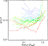 |
Fig. 8. Relative uncertainty on the temperature as a function of scaled radius, for the profiles defined with 30σ scientific S/N goal (Table 3). The profiles are colour coded as a function of the total S/N in the soft-band (Table 1), from blue (low S/N) to red (high S/N). |
Figure 9 shows the relative precision on each point of the temperature profile as a function of the corresponding S/N in that annular bin. There is a good correlation, justifying a posteriori the underlying assumption of the binning method. There is a dispersion with an apparent increased error with increasing temperature at a given S/N. As the S/N is defined in the soft band this is expected. The upper limit of the band is below the cut-off energy of the bremsstrahlung energy at E∼kT, in most cases. The soft band flux (and thus the S/N in that band) is therefore insensitive to temperature while, with increasing temperature, the energy cut-off moves to higher energy, where the instrument effective area decreases. As this sets the constraints on temperature, its precision also decreases at a given S/N.
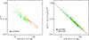 |
Fig. 9. Relation between S/N and fractional temperature uncertainty. Left: Relation between relative error on the temperature and S/N. Each point corresponds to a bin of a temperature profile. Right: Rescaled relation, including data from REXCESS at lower redshift. Points are colour coded according to their temperature, lower and higher kT being displayed in blue and red, respectively. |
Adding information from REXCESS to increase the redshift leverage, we found an empirical power law relation between the relative error, once rescaled as a function of T/(1 + z), and the S/N:
![$$ \begin{aligned} \frac{\Delta (T)}{T} \times \left[T_{5}/(1+z)\right]^{-0.51} = 0.11\,\times \left[\frac{\mathrm{S/N}}{30}\right]^{-1.09} \end{aligned} $$](/articles/aa/full_html/2024/08/aa48411-23/aa48411-23-eq14.gif)
where T5 is the temperature in units of 5 keV. This is illustrated on the right panel of Fig. 9. This relation can be used, for instance, to define the exposure times required to reach a given temperature precision from simple information on the surface brightness profile or the overall count rate.
5.2. Scaled temperature profiles
5.2.1. 3D temperature profiles
The 2D temperature profiles derived using the algorithm described above were deprojected and PSF-corrected as described in Bartalucci et al. (2018). In brief, each individual 2D profile was modelled with a 3D parametric model similar to that proposed by Vikhlinin et al. (2006), convolved with a response matrix that simultaneously takes into account projection and PSF redistribution. The weighting scheme introduced by Vikhlinin (2006) was used to correct for the bias introduced by fitting isothermal models to multi-temperature plasma. Fitting was undertaken with Bayesian maximum likelihood estimation and Markov chain Monte Carlo (MCMC) sampling, using emcee (Foreman-Mackey et al. 2013). The final deprojected, PSF-corrected profiles were derived from the best-fitting model temperature at the weighted radii corresponding to the 2D annular binning scheme. The left-hand panel of Fig. 10 shows the resulting 3D profiles scaled in terms of R500 and TX, the spectral temperature in the [0.15 − 0.75] R500 region, colour-coded as a function of mass. The individual 2D and 3D temperature profiles and associated best fitting models are shown in Appendix B.
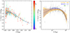 |
Fig. 10. Left: Deconvolved, deprojected, 3D temperature profiles of the EXCPReS sample, scaled by R500 and the spectral temperature in the [0.15 − 0.75] R500 region, colour-coded by total mass. The best-fitting analytical model (Eqs. 2–5) is overplotted. Right: Scaled 3D profiles of the EXCPReS sample (points with error bars) and best-fitting model (orange), compared to the best-fitting model to the scaled temperature profile of the REXCESS sample (blue). Envelopes indicate the radially-varying intrinsic scatter term. The dotted line shows the best-fitting model to the local cool core sample of Vikhlinin et al. (2006). |
5.2.2. Sample average profile
We fitted the scaled profiles Tm(x) = T(r)/TX with a model consisting of an analytical profile with a radially-varying intrinsic scatter term using the formalism described in Pratt et al. (2022):

with

with f(x) being described by the model proposed by Vikhlinin et al. (2006)
![$$ \begin{aligned} f(x) = T_0 \times \frac{({ y}+T_{\rm min}/T_0)}{({ y}+1)} \times \frac{(x/x_t)^{-a}}{\left[ 1+(x/x_t)^b\right]^{c/b}} \ \ ; \ { y}=\left(\frac{x}{x_{\rm cool}}\right)^{a_{\rm cool}}. \end{aligned} $$](/articles/aa/full_html/2024/08/aa48411-23/aa48411-23-eq17.gif)
Accounting for measurement errors, the probability of measuring a given scaled gas temperature, T, at given scaled radius, x, is
![$$ \begin{aligned} p(T|x)&= \mathcal{N} [\log {T_{\rm m}}(x),\sigma ^2(x) ]\end{aligned} $$](/articles/aa/full_html/2024/08/aa48411-23/aa48411-23-eq18.gif)
where 𝒩 is the log-normal distribution, while the variance, σ2(x), is the quadratic sum of the statistical error σstat on the measured log T(x), and of the intrinsic scatter on the median profile log Tm(x) at radius x, σint(x). As in Pratt et al. (2022), we used a non-analytical form for the intrinsic scatter, defining σint(x) at n equally-spaced points in log(x) with σint(x) at other radii being computed by spline interpolation. We used n = 7 between xmin = 0.01 and xmax = 1.
The likelihood of a set of scaled temperature profiles measured for a sample of i = 1, Nc clusters is:
![$$ \begin{aligned} \mathcal{L} = \prod _{i=0}^{N_{\rm c}} \prod _{j=0}^{ N_{\rm R}[i]} p\,(T_{i, j} \vert x_{i,j}), \end{aligned} $$](/articles/aa/full_html/2024/08/aa48411-23/aa48411-23-eq20.gif)
where NR[i] is the number of points of the profile of cluster i, and the quantity Ti, j = T[i, j]/TXi is the scaled temperature measured at each scaled radius xi, j = r[i, j]/R500, i, with T[i, j] and r[i, j] being the physical gas temperature and radius. The statistical error on log Ti, j is σstat, i, j. We fitted the data (i.e. the set of observed T[i, j] ) using a Bayesian maximum likelihood estimation with MCMC sampling. Using the emcee package developed by Foreman-Mackey et al. (2013), we maximised the log of the likelihood, which is expressed as:
![$$ \begin{aligned}&\ln {\mathcal{L} } = -0.5 \sum _{i,j} \left[ \ln {\sigma ^2_{\rm i,j} } + \frac{ \left(\log {T_{i,j}}- \log {T_{\mathrm{m}, i, j}} \right)^2 }{ \sigma ^2_{\rm i,j}} \right] \end{aligned} $$](/articles/aa/full_html/2024/08/aa48411-23/aa48411-23-eq21.gif)
The fit marginalises over a total of fifteen parameters: eight describing the shape of the median profile (Tmin, T0, xt, xcool, a, acool, b, c), and seven additional parameters describing the intrinsic scatter profile. We used flat priors on all parameters.
The orange envelope in Figure 10 shows the resulting best-fitting model overplotted on the EXCPReS data points. The best-fitting parameters for f(x) are as follows:
and given with their marginalised 68% uncertainties in Table 4. The marginalised posterior distributions of each parameter are shown in Fig. C.1. For comparison, we also show in Fig. 10 the best-fitting model obtained from fitting the 3D temperature profiles of the representative local X-ray-selected REXCESS sample (Pratt et al. 2007). Finally, we also overplot the best-fitting model to the local cool-core sample published by Vikhlinin et al. (2006). Outside the central region, the agreement between models is good, suggesting no evolution in the bulk temperature profile within the redshift range probed by the present samples. Agreement in the outer regions is expected from theoretical models of self-similarity. However, within the central ∼0.2 R500 region, there is a suggestion that the cool core sample of Vikhlinin et al. (2006) has a lower central temperature and a higher peak temperature than either of the representative samples. Here, comparison between samples is hampered by radial binning considerations, where cool core systems always have a finer binning than non-cool core systems because of their higher S/N (see Table 4). Further progress on this issue will necessitate careful treatment of the S/N in the central regions, and the inclusion of the dynamical state as an additional parameter (e.g. Bartalucci et al. 2019).
6. Summary and conclusions
In this paper, we introduce EXCPReS, a representative X-ray selected sample of 31 galaxy clusters at moderate redshifts (0.4 < z < 0.6), and spanning the full mass range (1014 < M500 < 1015 M⊙). EXCPReS was constructed to be an analogue of the low-redshift REXCESS sample (Böhringer et al. 2007).
We used the XMM-Newton observations of the EXCPReS sample to develop and test a new method to produce optimally binned X-ray temperature profiles. The method uses a dynamic programming algorithm based on partitioning of the SX-bin range to obtain a new binning scheme that fulfils a given S/N threshold criterion out to large radius. Additional optional criteria can be included, including logarithmic radial binning, or setting a minimum number of SX-bins to be included in each kT-bin. The method aims at maximising the number of temperature profile bins out to the largest (optionally required) radius. A user-chosen minimum number of bins can be used as a fallback solution for cases with low S/N: in this case, the algorithm maximises the S/N of all bins simultaneously.
We demonstrated the efficiency of our method using the EXCPReS sample, which contains data sets covering a wide range of S/N. The expected correlation between the S/N in kT-bins and the relative error on the temperature shows very little dispersion, but exhibits a clear trend with global temperature. Combining the results from EXCPReS and REXCESS, we derived a relation between the relative uncertainty in kT-bins with respect to the soft-band SX S/N within these kT-bins, and its dependence on global temperature and redshift (Eq. 1). This relation provides a useful tool for exposure time calculation in X-ray observations, allowing one to obtain an estimate of a given relative error on the ICM temperature measurements, based only on the knowledge of the soft-band number counts.
The optimally binned 2D temperature profiles were PSF-deconvolved and deprojected to derive the 3D profiles. Once scaled by R500 and TX, the temperature in the [0.15 − 0.75] R500 region, the 3D EXCPReS temperature profiles exhibit a clear self similar behaviour beyond the core region and increased dispersion towards the centre. We obtained a mean temperature profile for the EXCPReS sample and compared to that from the local X-ray selected REXCESS sample. This comparison shows no obvious sign of evolution in the average temperature profile shape in the redshift range probed in the present study.
In a forthcoming paper we will further investigate the 3D thermodynamic profiles of the EXCPReS sample and how the global properties scale, with respect to the expected self similar evolution and to the cluster mass.
MCXC-II also includes additional MACS clusters recovered from non-catalogue studies (the MACS_MISC sub-catalogue). We discarded them in this study as their X-ray selection function is not defined. In the redshift range under consideration, this concerns four clusters from the on-going extension of the MACS survey in the South (Repp & Ebeling 2018).
We can think of the problem of partitioning (n + 1) SX input bins into (r + 1) kT output bins as choosing r amongst the nSX-bin boundaries as kT-bin boundaries. The number of ways to do so is then  , where nCr = n!/r!/(n − r)! are the binomial coefficients appearing on the n-th row of Pascal’s Triangle, whose sum is 2n.
Suppose that OP[a, c] is Partition [a, b]∪Partition [b + 1, c], but OP[a, b] is not Partition [a, b] but rather Partition* [a, b]. Then Partition* [a, b]∪Partition [b + 1, c] would give higher S/N than Partition [a, b]∪Partition [b + 1, c], contradicting the initial assertion that the latter is OP[a, c].
Acknowledgments
Santa, xeus (our local computing facility) for crashing only once during all these years. We would like to thank the people and funding agencies who have supported us over the many years that it has taken us to write this paper. We acknowledge in particular long-term support from CNRS/INSU and from the French Centre National d’Études Spatiales (CNES). The results reported in this article are based on data obtained from the XMM-Newton observatory, an ESA science mission with instruments and contributions directly funded by ESA Member States and NASA.
References
- Anokhin, S. G. 2008, Adv. Space Res., 42, 576 [NASA ADS] [CrossRef] [Google Scholar]
- Arnaud, M. 2008, The X-ray Universe 2008, 191 [Google Scholar]
- Arnaud, M., Neumann, D. M., Aghanim, N., et al. 2001, A&A, 365, L80 [NASA ADS] [CrossRef] [EDP Sciences] [Google Scholar]
- Arnaud, M., Pointecouteau, E., & Pratt, G. W. 2007, A&A, 474, L37 [CrossRef] [EDP Sciences] [Google Scholar]
- Arnaud, M., Pratt, G. W., Piffaretti, R., et al. 2010, A&A, 517, A92 [CrossRef] [EDP Sciences] [Google Scholar]
- Art, L., & Mauch, H. 2007, Dynamic Programming: A Computational Tool, Studies in Computational Intelligence (Berlin, Heidelberg: Springer) [Google Scholar]
- Baldi, A., Ettori, S., Mazzotta, P., Tozzi, P., & Borgani, S. 2007, ApJ, 666, 835 [NASA ADS] [CrossRef] [Google Scholar]
- Baldi, A., Ettori, S., Molendi, S., & Gastaldello, F. 2012, A&A, 545, A41 [NASA ADS] [CrossRef] [EDP Sciences] [Google Scholar]
- Bartalucci, I., Arnaud, M., Pratt, G. W., et al. 2017, A&A, 598, A61 [NASA ADS] [CrossRef] [EDP Sciences] [Google Scholar]
- Bartalucci, I., Arnaud, M., Pratt, G. W., & Le Brun, A. M. C. 2018, A&A, 617, A64 [NASA ADS] [CrossRef] [EDP Sciences] [Google Scholar]
- Bartalucci, I., Arnaud, M., Pratt, G. W., Démoclès, J., & Lovisari, L. 2019, A&A, 628, A86 [EDP Sciences] [Google Scholar]
- Bleem, L. E., Stalder, B., de Haan, T., et al. 2015, ApJS, 216, 27 [Google Scholar]
- Böhringer, H., Voges, W., Huchra, J. P., et al. 2000, ApJS, 129, 435 [Google Scholar]
- Böhringer, H., Schuecker, P., Guzzo, L., et al. 2004, A&A, 425, 367 [NASA ADS] [CrossRef] [EDP Sciences] [Google Scholar]
- Böhringer, H., Schuecker, P., Pratt, G. W., et al. 2007, A&A, 469, 363 [NASA ADS] [CrossRef] [EDP Sciences] [Google Scholar]
- Burenin, R. A., Vikhlinin, A., Hornstrup, A., et al. 2007, ApJS, 172, 561 [Google Scholar]
- Burke, D. J., Collins, C. A., Sharples, R. M., Romer, A. K., & Nichol, R. C. 2003, MNRAS, 341, 1093 [NASA ADS] [CrossRef] [Google Scholar]
- Cormen, T. H., Leiserson, C. E., Rivest, R. L., & Stein, C. 2009, Introduction to Algorithms (MIT Press and McGraw-Hill) [Google Scholar]
- Croston, J. H., Arnaud, M., Pointecouteau, E., & Pratt, G. W. 2006, A&A, 459, 1007 [NASA ADS] [CrossRef] [EDP Sciences] [Google Scholar]
- De Grandi, S., & Molendi, S. 2002, ApJ, 567, 163 [CrossRef] [Google Scholar]
- Ebeling, H., Barrett, E., Donovan, D., et al. 2007, ApJ, 661, L33 [Google Scholar]
- Ebeling, H., Edge, A. C., Mantz, A., et al. 2010, MNRAS, 407, 83 [NASA ADS] [CrossRef] [Google Scholar]
- Foreman-Mackey, D., Hogg, D. W., Lang, D., & Goodman, J. 2013, PASP, 125, 306 [Google Scholar]
- Gioia, I. M., Maccacaro, T., Schild, R. E., et al. 1990, ApJS, 72, 567 [NASA ADS] [CrossRef] [Google Scholar]
- Hasselfield, M., Hilton, M., Marriage, T. A., et al. 2013, JCAP, 2013, 008 [Google Scholar]
- Henry, J. P. 2004, ApJ, 609, 603 [NASA ADS] [CrossRef] [Google Scholar]
- Henry, J. P., Mullis, C. R., Voges, W., et al. 2006, ApJS, 162, 304 [NASA ADS] [CrossRef] [Google Scholar]
- Horner, D. J., Perlman, E. S., Ebeling, H., et al. 2008, ApJS, 176, 374 [NASA ADS] [CrossRef] [Google Scholar]
- Kalberla, P. M. W., Burton, W. B., Hartmann, D., et al. 2005, A&A, 440, 775 [NASA ADS] [CrossRef] [EDP Sciences] [Google Scholar]
- Kay, S. T., & Pratt, G. W. 2022, Handbook of X-ray and Gamma-ray Astrophysics, eds. C. Bambi, & A. Santangelo, 100 [Google Scholar]
- Kotov, O., & Vikhlinin, A. 2005, ApJ, 633, 781 [NASA ADS] [CrossRef] [Google Scholar]
- Kravtsov, A. V., & Borgani, S. 2012, ARA&A, 50, 353 [Google Scholar]
- Kravtsov, A. V., Vikhlinin, A., & Nagai, D. 2006, ApJ, 650, 128 [Google Scholar]
- Leccardi, A., & Molendi, S. 2008, A&A, 486, 359 [NASA ADS] [CrossRef] [EDP Sciences] [Google Scholar]
- Lovisari, L., & Maughan, B. J. 2022, Handbook of X-ray and Gamma-ray Astrophysics, eds. C. Bambi, & A. Santangelo, 65 [Google Scholar]
- Lovisari, L., Reiprich, T. H., & Schellenberger, G. 2015, A&A, 573, A118 [NASA ADS] [CrossRef] [EDP Sciences] [Google Scholar]
- Lumb, D. H., Bartlett, J. G., Romer, A. K., et al. 2004, A&A, 420, 853 [NASA ADS] [CrossRef] [EDP Sciences] [Google Scholar]
- Mann, A. W., & Ebeling, H. 2012, MNRAS, 420, 2120 [NASA ADS] [CrossRef] [Google Scholar]
- Mantz, A. B., Allen, S. W., Morris, R. G., & Schmidt, R. W. 2016, MNRAS, 456, 4020 [NASA ADS] [CrossRef] [Google Scholar]
- Markevitch, M. 1998, ApJ, 504, 27 [Google Scholar]
- McDonald, M., Benson, B. A., Vikhlinin, A., et al. 2014, ApJ, 794, 67 [Google Scholar]
- Melin, J. B., Bartlett, J. G., & Delabrouille, J. 2006, A&A, 459, 341 [NASA ADS] [CrossRef] [EDP Sciences] [Google Scholar]
- Mullis, C. R., McNamara, B. R., Quintana, H., et al. 2003, ApJ, 594, 154 [NASA ADS] [CrossRef] [Google Scholar]
- Perlman, E. S., Horner, D. J., Jones, L. R., et al. 2002, ApJS, 140, 265 [NASA ADS] [CrossRef] [Google Scholar]
- Piffaretti, R., Arnaud, M., Pratt, G. W., Pointecouteau, E., & Melin, J.-B. 2011, A&A, 534, A109 [NASA ADS] [CrossRef] [EDP Sciences] [Google Scholar]
- Planck Collaboration VIII. 2011, A&A, 536, A8 [NASA ADS] [CrossRef] [EDP Sciences] [Google Scholar]
- Planck Collaboration XXIX. 2014, A&A, 571, A29 [NASA ADS] [CrossRef] [EDP Sciences] [Google Scholar]
- Planck Collaboration XXVII. 2016, A&A, 594, A27 [NASA ADS] [CrossRef] [EDP Sciences] [Google Scholar]
- Pratt, G. W., & Arnaud, M. 2003, A&A, 408, 1 [CrossRef] [EDP Sciences] [Google Scholar]
- Pratt, G. W., Böhringer, H., Croston, J. H., et al. 2007, A&A, 461, 71 [NASA ADS] [CrossRef] [EDP Sciences] [Google Scholar]
- Pratt, G. W., Arnaud, M., Piffaretti, R., et al. 2010, A&A, 511, A85 [NASA ADS] [CrossRef] [EDP Sciences] [Google Scholar]
- Pratt, G. W., Arnaud, M., Maughan, B. J., & Melin, J. B. 2022, A&A, 665, A24 [NASA ADS] [CrossRef] [EDP Sciences] [Google Scholar]
- Repp, A., & Ebeling, H. 2018, MNRAS, 479, 844 [NASA ADS] [Google Scholar]
- Romer, A. K., Nichol, R. C., Holden, B. P., et al. 2000, ApJS, 126, 209 [NASA ADS] [CrossRef] [Google Scholar]
- Rykoff, E. S., Rozo, E., Hollowood, D., et al. 2016, ApJS, 224, 1 [NASA ADS] [CrossRef] [Google Scholar]
- Sadibekova, T., Arnaud, M., Pratt, G. W., Tarrío, P., & Melin, J. B. 2024, A&A, 688, A187 [NASA ADS] [CrossRef] [EDP Sciences] [Google Scholar]
- Schaye, J., Crain, R. A., Bower, R. G., et al. 2015, MNRAS, 446, 521 [Google Scholar]
- Schaye, J., Kugel, R., Schaller, M., et al. 2023, MNRAS, 526, 4978 [NASA ADS] [CrossRef] [Google Scholar]
- Sun, M., Voit, G. M., Donahue, M., et al. 2009, ApJ, 693, 1142 [NASA ADS] [CrossRef] [Google Scholar]
- Ulmer, M. P., Adami, C., Covone, G., et al. 2005, ApJ, 624, 124 [NASA ADS] [CrossRef] [Google Scholar]
- Vikhlinin, A. 2006, ApJ, 640, 710 [NASA ADS] [CrossRef] [Google Scholar]
- Vikhlinin, A., McNamara, B. R., Forman, W., et al. 1998, ApJ, 502, 558 [Google Scholar]
- Vikhlinin, A., Markevitch, M., Murray, S. S., et al. 2005, ApJ, 628, 655 [Google Scholar]
- Vikhlinin, A., Kravtsov, A., Forman, W., et al. 2006, ApJ, 640, 691 [Google Scholar]
- Vogelsberger, M., Genel, S., Springel, V., et al. 2014, MNRAS, 444, 1518 [Google Scholar]
- Wen, Z. L., & Han, J. L. 2015, ApJ, 807, 178 [Google Scholar]
Appendix A: Clusters with XMM-Newton observations not included in EXCPReS
The MCXC clusters in the low-luminosity sample (L500 < 4 × 1044 ergs s−1) with archival observations, but not included in the EXCPReS sample, are listed in Tab. A.1. The table also gives the OBSID of the XMM-Newton observation and the reference of relevant published XMM-Newton analysis. We further analysed the archival data of some of the clusters.
Clusters in the 0.4 < z < 0.6 range with XMM-Newton archival data but not included in the EXCPReS sample. The clusters are ordered by increasing redshift. Columns are 1-2: Cluster MCXC name and other name, 3: Detection survey, 4: Redshift, 5: XMM-Newton OBSID, 6: Reference to relevant publication or present work; (1) Baldi et al. (2012); (2) Anokhin (2008); (3) Lumb et al. (2004); and (4) Ulmer et al. (2005)
MCXC J1002.6-0808 was observed in the framework of our Large Programme #030258. The observation revealed that MCXC J1002.6-0808 is a point source, which is also confirmed by the Chandra image.
Our study of the image of MCXC J1419.8+0634 shows that it is a bimodal cluster, thus not suitable for radial analysis.
We require a minimal S/N ratio of S/N = 20, needed to derive a temperature profile as shown by our work. The other clusters could not be retained because the archival observations are not deep enough:
-
The observations of the two EMSS clusters, MCXC J0305.3+1728 (z = 0.425) and MCXC J2056.3-0437 (z = 0.583, are shallow, with clean observing time of ∼10 ksec and 12 ksec, respectively (Baldi et al. 2012, their Tab.1). The error on the global temperature is ±15%. Baldi et al. (2012) were only able to extract the temperature in 2 bins up to 0.4R500 for MCXC J2056.3-0437.
-
The observations of MCXC J1325.5-3825, MCXC J0505.3-2849, MCXC J1354.2-0221, MCXC J0847.1+3449 and MCXC J0337.7-2522 were early follow up of SHARC clusters to meant to measure a global temperature and the luminosity, published by Lumb et al. (2004). Our full re-analysis of MCXC J0505.3-2849, the best measured cluster of the list, gives a S/N500 = 20. The observations of the other clusters are at lower S/N, taking into account the precision on the observed flux (their table 5). MCXC J1325.5-3825 falls in the field of view of an observation centered on IRAS 13224−3809, a very bright Seyfert galaxy. Many more observations have become available over the years, but only in Window mode, and centred on the galaxy. Note that the two other clusters of their sample at 0.4 < z < 0.6, MCXC J1120.1+4318 and MCXC J1701.3+6414 (re-observed by XMM-Newton), are included in the EXCPReS sample.
-
Together with MCXC J0337.7-2522 studied by Lumb et al. (2004), MCXC J2202.7-1902 and MCXC J0858.4+1357 are the three 0.4 < z < 0.6 clusters with the lowest luminosities, L500 < 1044ergs/s, observed by XMM-Newton. Anokhin (2008) gives a temperature of about 3 keV for MCXC J2202.7-1902 and MCXC J0858.4+1357. From our analysis of the surface brightness profiles and global properties, we derived a S/N ratio of S/N = 15 and S/N500 = 19, respectively. This entails that the EXCPReS selection could not be extended below L500 = 1044ergs/s.
-
MCXC J0056.9-2740 (z = 0.56) falls in the field of the programme ‘A shallow XMM survey of AAT 2DF fields SSC_32’ (PI M. Watson). This includes two short observations of 7.2 ksec (highly flared) and 8.9 ksec, respectively. This is too shallow to obtain spatially resolved spectroscopy of the z = 0.56 cluster and indeed the examination of the EPIC image shows that the cluster is poorly detected. MCXC J0056.9-2740 coincides with the source 4XMM J005657.1-274028, detected at 13 σ in the 4XMM-DR13 catalogue.
-
MCXC J1205.8+4429 is a fossil group, as shown by Ulmer et al. (2005). From their Table 2, the S/N of the group observation is S/N ∼ 21 and there is a ±10% error on the global temperature.
In conclusion, the final selection for the low luminosity box of EXCPReS includes clusters with 0.44 < z < 0.56 and 1044 < L500 < 4 × 1044 ergs s−1. Four further objects with archival data fall in that range but are not retained: three SHARC clusters published by Lumb et al. (2004) since the exposure is not deep enough, and a 160SD/WARPS object which is false detection.
Appendix B: Individual temperature profiles
Individual temperature profiles of the EXCPReS sample are shown in Fig. B.1 and B.2. In all panels, the black points with error bars show the annular temperature measurements. Solid green lines show the best fitting 3D temperature model, with its uncertainty indicated by the dashed green lines. Red lines show the 2D reprojection of the best fitting 3D model, and dashed red lines the associated uncertainty.
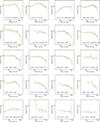 |
Fig. B.1. Individual temperature profiles of the EXCPReS sample. Black points with error bars show the annular temperature measurements. Green lines show the best fitting 3D temperature model. Red lines show the 2D reprojection of the best fitting 3D model. The model uncertainties are indicated by dashed lines. |
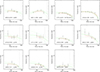 |
Fig. B.2. continued. |
Appendix C: Posteriors
Marginalised posterior likelihood for the parameters of the best-fitting temperature profile model to the EXCPReS data, as detailed in Sect. 5.2.
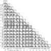 |
Fig. C.1. Marginalised posterior likelihood for the parameters of the best-fitting temperature profile model to the EXCPReS data. |
All Tables
Variations to the standard binning algorithm applied to each object in our sample.
Clusters in the 0.4 < z < 0.6 range with XMM-Newton archival data but not included in the EXCPReS sample. The clusters are ordered by increasing redshift. Columns are 1-2: Cluster MCXC name and other name, 3: Detection survey, 4: Redshift, 5: XMM-Newton OBSID, 6: Reference to relevant publication or present work; (1) Baldi et al. (2012); (2) Anokhin (2008); (3) Lumb et al. (2004); and (4) Ulmer et al. (2005)
All Figures
|
Fig. 1. Distribution in the M − z plane of the EXCPReS sample (red points). The local X-ray-selected REXCESS sample (Böhringer et al. 2007) is shown with blue points. Shown for comparison are confirmed clusters from major SZE surveys from which individual spatially resolved temperature profiles are measurable: Filled circles: Planck clusters (Planck Collaboration VIII 2011; Planck Collaboration XXIX 2014; Planck Collaboration XXVII 2016). Crosses: SPT (Bleem et al. 2015). Plus symbols: ACT (Hasselfield et al. 2013). |
| In the text | |
|
Fig. 2. Distribution of the MCXC clusters in the z–L500 plane (Piffaretti et al. 2011). Redshift and L500, the luminosity within R500, are from the updated MCXC catalogue (Sadibekova et al. 2024). Each cluster is colour-coded according to the survey from which the luminosity is taken. Clusters with XMM-Newton observations are marked with red circles and those included in the EXCPReS sample are marked with red boxes. The dotted lines mark the [0.1–2.4] keV band flux taking into account the Kz correction for a typical gas temperature of 5 keV. Levels are separated by 2 dex, from 1.25 × 10⁻¹³ up to 4 × 10⁻¹² ergs s−1 cm−2. |
| In the text | |
|
Fig. 3. Gallery of the XMM-Newton images, extracted in the [0.3–2] keV energy band, for the 31 clusters of the sample, ordered by decreasing mass. Image sizes are 3θ500 on a side, where θ500 is estimated from the M500–YX relation. Images are corrected for surface brightness dimming with z, divided by the emissivity in the energy band, taking into account galactic absorption and instrument response, and scaled according to the self-similar model. The colour table is the same for all clusters, so that the images would be identical if clusters obeyed self-similarity. |
| In the text | |
|
Fig. 4. Gallery of X-ray images for the clusters of the sample, continued. |
| In the text | |
|
Fig. 5. Visual representation of the problem of binning surface-brightness (SX) bins into temperature-profile (kT) bins. Left: SX profile of RXJ0856.1+3756 in the [0.3–2] keV band, extracted in 3 |
| In the text | |
|
Fig. 6. Example binning solutions. Left: Initial binning solution for the galaxy cluster RXJ0856.1+3756 (solid white steps) from the algorithm specified in Sect. 4.3. The solid green curve delineates a 30σ S/N requirement. It shows that indefinitely adding more input SX bins to an output kT bin is suboptimal. The cyan steps represent |
| In the text | |
|
Fig. 7. Two algorithm variations. The S/N landscape is shown here uncapped for illustration, but it is capped in the binning algorithm as described in Sect. 4.3.2. In both panels, the solid curve represents a S/N of 30σ. Left: Modified S/N landscape and the resulting binning solution for the galaxy cluster CL0016+16. Here, the output kT bins are required to fulfil four simultaneous criteria: (1) to have a target S/N of 30σ (denoted by the solid curve); (2) to have a minimum S/N ≥3σ; (3) to include at least two SX bins; and (4) to increase in width with a logarithmic factor of 1.2. Right: Optimal binning for the low S/N cluster RXJ0030.5+2618, obtained from fixing the number of output kT bins to four and maximising their resulting S/N (see Sect. 4.3.3). |
| In the text | |
|
Fig. 8. Relative uncertainty on the temperature as a function of scaled radius, for the profiles defined with 30σ scientific S/N goal (Table 3). The profiles are colour coded as a function of the total S/N in the soft-band (Table 1), from blue (low S/N) to red (high S/N). |
| In the text | |
|
Fig. 9. Relation between S/N and fractional temperature uncertainty. Left: Relation between relative error on the temperature and S/N. Each point corresponds to a bin of a temperature profile. Right: Rescaled relation, including data from REXCESS at lower redshift. Points are colour coded according to their temperature, lower and higher kT being displayed in blue and red, respectively. |
| In the text | |
|
Fig. 10. Left: Deconvolved, deprojected, 3D temperature profiles of the EXCPReS sample, scaled by R500 and the spectral temperature in the [0.15 − 0.75] R500 region, colour-coded by total mass. The best-fitting analytical model (Eqs. 2–5) is overplotted. Right: Scaled 3D profiles of the EXCPReS sample (points with error bars) and best-fitting model (orange), compared to the best-fitting model to the scaled temperature profile of the REXCESS sample (blue). Envelopes indicate the radially-varying intrinsic scatter term. The dotted line shows the best-fitting model to the local cool core sample of Vikhlinin et al. (2006). |
| In the text | |
|
Fig. B.1. Individual temperature profiles of the EXCPReS sample. Black points with error bars show the annular temperature measurements. Green lines show the best fitting 3D temperature model. Red lines show the 2D reprojection of the best fitting 3D model. The model uncertainties are indicated by dashed lines. |
| In the text | |
|
Fig. B.2. continued. |
| In the text | |
|
Fig. C.1. Marginalised posterior likelihood for the parameters of the best-fitting temperature profile model to the EXCPReS data. |
| In the text | |
Current usage metrics show cumulative count of Article Views (full-text article views including HTML views, PDF and ePub downloads, according to the available data) and Abstracts Views on Vision4Press platform.
Data correspond to usage on the plateform after 2015. The current usage metrics is available 48-96 hours after online publication and is updated daily on week days.
Initial download of the metrics may take a while.