© The Authors 2024

1. Introduction

The theory of diffusive shock acceleration (DSA) was introduced in four independent papers and was initially formulated in two alternative approaches. The first approach was through the kinetic equation (Krymskii 1977; Axford et al. 1977; Blandford & Ostriker 1978), while the second was based on the microscopic description (Bell 1978a). Although Bell’s approach is quite intuitive, most of the results related to DSA have been derived by considering the diffusion–convection equation.

The approach of Bell (1978a) deserves more attention as it may be used to derive the known solutions of the kinetic equation and help with new problems. To illustrate the possibilities of the Bell approach, we obtained the solution of Blasi (2002) for the non-linear acceleration (NLA) problem, which we present in Sect. 2.

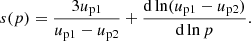
It has been known for a long time that the spectrum of accelerated particles is affected by the non-uniformity of the plasma flow (e.g. Bogdan & Volk 1983. The NLA solution indeed reflects the non-uniform velocity distribution upstream of the shock, where the particles of higher energies diffuse farther upstream and are scattered back to the shock by scattering centres whose speed differs from the speed of the centres affecting particles of the smaller momenta, which are able to penetrate to shorter distances in the preshock region. This leads to the formation of a concave particle spectrum (e.g. Malkov & Drury 2001; Blasi 2002) instead of a simple power-law derived from the linear approach, where the plasma speed u is considered uniform both upstream and downstream of the shock (e.g. Drury 1983).

The common boundary condition for DSA problems is a zero gradient of the flow velocity behind the shock. However, if du/dx ≠ 0 in the upstream medium affects the particle spectrum shape, this leads us to wonder what the effects might be of also considering a non-zero gradient downstream.

The diffusion length of particles accelerated at the shock can reach ∼0.1 of the shock radius. At this distance downstream in real objects – for example, in supernova remnants (SNRs) –, the flow velocity differs from the immediate post-shock value. Hence, we may expect a ‘downstream’ effect similar to the ‘upstream’ one from the non-linear approach. Moreover, it is known from self-similar solutions (e.g. Chevalier 1982; Sedov 1959) and hydrodynamic simulations (e.g. recent Patnaude et al. (2015), Orlando et al. (2015), Gabler et al. (2021) for the case of the core-collapse supernovae (SNe) and Ferrand et al. (2019, 2021) for the type Ia SNe), that the structure of the flow undergoes essential changes during the early evolution of SNRs. Therefore, we may expect the shape of the spectrum of accelerated particles to vary with time due to the variable non-uniformity of the downstream flow.

In the present paper, we address this effect in the framework of the Bell approach to particle acceleration at shocks. Section 3 presents details of our motivation to answer this question, where we consider the spatial profiles of the plasma velocity behind the SNR shocks from numerical simulations. Appendix A includes an animation of the evolution of the flow speed. In Sect. 4, we use the generalised description of the Bell approach from Sect. 2 to DSA with the non-uniform downstream flow. We consider two practical cases: test-particle and non-linear (NLA) acceleration of particles. Appendix B provides relevant details of the presented derivations. In Sect. 5, we discuss possible scenarios where the effect could be visible. Our conclusions are presented in Sect. 6. Appendix C presents the derivation of the same solution as in Sect. 4 but this time by solving the kinetic equation.

2. NLA in the framework of the Bell approach

Let us consider the shock reference frame with the shock at the coordinate x = 0. In this frame, the flow velocity of the shock u is in the positive x direction. Particles are accelerated by repeating the acceleration cycle multiple times, that is, crossing the shock from downstream (x > 0, index ‘2’) to upstream (x < 0, index ‘1’) and then again to downstream. The approach of Bell (1978a) consists in finding the increase in the particle momentum per cycle and the probability of participating in the next acceleration cycle, then considering many repetitions. We refer the reader to Sect. 3.3 of Jones & Ellison (1991) for the extended formulation of the approach. In the present section, we generalise this approach to the modified shock.

The main idea behind DSA is that the spatial structure of the flow determines the change in the particle momentum ṗ ≡ dp/dt:

$$\begin{array}{c}\hfill \dot{p}=-\frac{p}{3}\frac{\mathrm{d}u}{\mathrm{d}x}.\end{array}$$(1)

The average momentum gain is derived by integration of this expression,

$$\begin{array}{c}\hfill {\displaystyle \frac{\mathrm{\Delta }p}{p}=-\frac{1}{3}{\displaystyle {\int }_{x_a}^{x_b}}\frac{\mathrm{d}u}{\mathrm{d}x}\frac{\mathrm{d}x}{v_{\mathrm{x}}},}\end{array}$$(2)

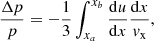
where v_x = dx/dt is the projection of the particle velocity v on the x-axis, and by averaging over the flux. The classic formula

$$\begin{array}{c}\hfill {\displaystyle \frac{\mathrm{\Delta }p}{p}=\frac{4}{v}\frac{u_1-u_2}{3}}\end{array}$$(3)

comes from (2) for any x_a < 0 and x_b > 0 if we assume that the upstream u₁(x) and the downstream u₂(x) velocities of the flow are uniform in their domains.

Under NLA conditions, the pressure of accelerated particles modifies the structure of the flow upstream of the shock, creating some profile u₁(x). The pressure of these particles downstream is negligible compared to the thermal pressure, and so the uniformity of u₂(x) = const remains unaffected.

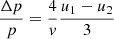
Let us first consider the problem in a simplified and more intuitive way. We assume that particles with the momentum p can move away from the shock to a maximum distance |x_p| upstream, where the flow speed is u_p1 = u₁(x_p) (Blasi 2002). Changing x_a to x_p in Eq. (2), we arrive at the formula (for more accurate derivation, refer to Sect. 4.1)

$$\begin{array}{c}\hfill {\displaystyle \frac{\mathrm{\Delta }p}{p}=\frac{4}{v}\frac{u_{\mathrm{p}1}-u_2}{3}.}\end{array}$$(4)

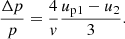
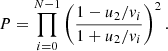
In order to participate in the next acceleration cycle, the particle should return to the shock from downstream against the flow direction; that is, its velocity component v_x should be −v_x > u₂. Therefore, the ratio of particle fluxes in the positive and negative x directions gives the probability of continuing acceleration for particles with an isotropic distribution of v (Jones & Ellison 1991)

$$\begin{array}{c}\hfill P={\left(\frac{1-u_2/v}{1+u_2/v}\right)}^2.\end{array}$$(5)

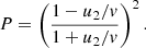
The probability to participate in at least N number of cycles is

$$\begin{array}{c}\hfill P={\displaystyle \prod _{i=0}^{N-1}}{\left(\frac{1-u_2/v_i}{1+u_2/v_i}\right)}^2.\end{array}$$(6)

Decomposition of the logarithm of P to the first order on u₂/v_i results in

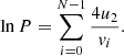$$\begin{array}{c}\hfill lnP={\displaystyle \sum _{i=0}^{N-1}}\frac{4u_2}{v_i}.\end{array}$$(7)

The original approach generalised the equation for the momentum increase (4) to N cycles, and its logarithm is decomposed to first order in u₂/v_i. We instead express 4/v_i from Eq. (4) and use this to substitute (7). Then, considering that the ratio Δp_i/p_i ∼ u₂/c ≪ 1 is small for relativistic particles and the number N is high, we make a transition from the summation to the integration: ∑Δp_i/p_i → ∫dp′/p′. After that, we obtain the probability for a particle to be accelerated to momentum p (or higher) from the injection momentum p_o on the steady background of the non-uniform profile of the flow velocity upstream:

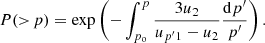$$\begin{array}{c}\hfill P(>p)=exp(-{\displaystyle {\int }_{p_{\mathrm{o}}}^p}\frac{3u_2}{u_{p^{\prime }1}-u_2}\frac{\mathrm{d}{p}^{\prime }}{p^{\prime }}).\end{array}$$(8)

This probability and the definition of the isotropic distribution function f_o(p) (Jones & Ellison 1991),

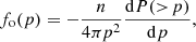$$\begin{array}{c}\hfill {\displaystyle f_{\mathrm{o}}(p)=-\frac{n}{4\pi p^2}\frac{\mathrm{d}P(>p)}{\mathrm{d}p},}\end{array}$$(9)

where index ‘o’ refers to the shock location (x = 0) and n is the number density of particles participating in the acceleration process by returning from downstream, results in the same steady-state distribution function of accelerated particles at the modified shock as derived by Blasi (2002) from the alternative approach of solving the kinetic equation,

$$\begin{array}{c}\hfill {\displaystyle f_{\mathrm{o}}(p)=\frac{\eta n_1}{4\pi p_{\mathrm{o}}^3}\frac{3u_1}{u_{\mathrm{p}1}-u_2}exp[-{\displaystyle {\int }_{p_0}^p}\frac{3u_{p^{\prime }1}}{u_{p^{\prime }1}-u_2}\frac{\mathrm{d}{p}^{\prime }}{p^{\prime }}],}\end{array}$$(10)

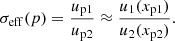
where η is the injection efficiency, and n₁ and u₁ should be taken at the same point – for example, in the immediate preshock location (at x = −0). It is clear that the shape of the particle spectrum depends on the effective compression factor σ_eff(p) = u_p1/u₂, which is ‘seen’ by particles with momentum p. The function (10) transforms to the power-law test-particle version if we assume that the flow velocity upstream is uniform, meaning the same convergence of the flow for particles of any momentum: σ_eff(p) = u₁/u₂. The non-linearity of this solution lies in the fact that σ_eff(p) itself depends on f(p), which requires another equation for these two functions. Blasi (2002) developed a way to relate σ_eff(p) to f(p) by considering the hydrodynamics of the flow. In their notation, σ_eff(p) = R_totU(p), where R_tot = u₀/u₂ represents the total compression factor of the shock and u₀ is the flow speed far upstream.

3. Profiles of the flow velocity

Studies of cosmic-ray-modified shocks demonstrate that the spatial non-uniformity of the plasma velocity upstream of the shock affects the shape of the momentum distribution of accelerated particles. It is natural to ask how the downstream flow structure modifies the particle spectrum. Numerical simulations of CR acceleration, which accounts for the complex hydrodynamic structure of the flow inside SNRs, demonstrate that the volume-averaged CR spectra can have a variety of possible shapes (e.g. Telezhinsky et al. 2012, 2013; Brose et al. 2020). In the present paper, we would like to consider the effect of the non-uniform flow in the vicinity of a single shock where the CR acceleration takes place.

The length scales involved in the particle acceleration at the forward shock are of the order of the diffusion length, which may eventually be up to a few times 0.1R, where R is the SNR radius. Most of the mass swept up by the forward shock is located immediately behind the adiabatic shock within about 10% of the radius. The ratio of densities is ρ(0.9R)/ρ(R) = 0.49 for the Sedov shock in the uniform medium. The variation of the flow velocity in the laboratory reference frame is not as strong, that is, v(0.9R)/v(R) = 0.82, but it is not negligible.

The leading motivation for the present study is the fact that the velocity of the flow u(x) is non-uniform downstream of the shock on the length scale involved in the particle acceleration; indeed it varies spatially from the value u₂ at x = +0 in accordance with the profile determined by the hydrodynamics. However, the length scale is small enough to avoid considering the effect of the shock curvature on particle acceleration. In fact, the distance 0.1R on the SNR surface corresponds to the sector with a central angle in arctan(0.1) = 5.7 degrees. Therefore, we can consider the one-dimensional acceleration problem within such a small sector with a plane shock.

For a presentation of the profiles u(x) we can expect downstream, we refer to our previous paper (Petruk et al. 2021). There, we investigate the MHD evolution of the remnants of three SN models, namely thermonuclear SNIa, and two core-collapse SNe: SNIc and SNIIP. We adopted a uniform ISM to model the type SNIa explosion, whereas the core-collapse SNe evolved in a circumstellar bubble with a density shaped by ρ_CS = Dr⁻², where the value of D depends on the explosion model. Core-collapse SNe produce a range of explosion conditions, unlike the thermonuclear explosion of a WD star (SNIa event). To account for this, we selected the two most representative cases, that is, a blue supergiant (SNIc) and a red supergiant (SNIIP) undergoing the core collapse. The SNIc and SNIIP models differ in the effective explosion mass and number density of a wind-blown bubble. We performed all numerical simulations with the PLUTO MHD code (Mignone et al. 2007, 2012). The spherically symmetric uniform grid has 20 000 zones, providing a very detailed spatial resolution during the entire simulation period. Petruk et al. (2021) provide more details on the technical model setup and on initial conditions for the explosion models.

Figure 1 shows the spatial distributions of the flow speed for the three models at the age of 500 yr and for three different SNR ages in the case of the SNIa model. The plots in the left column correspond to the laboratory frame, and those in the right column correspond to the shock frame. The velocity profile u₂(x) may rise or decline with distance from the shock. The distribution evolves with time, for example, changing from a decreasing to an increasing function of x in the SNIa model (Fig. 1 bottom right plot). The animation in Appendix A shows the detailed evolution of the velocity distributions up to 10 000 yr in these three models.

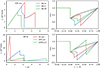Fig. 1. Profiles of the flow velocity v(r) in the observer reference frame (left) and u(x) in the shock reference frame (right) for the three models of SNRs. Upper row: Three SNe models at 500 yr. Lower row: SNIa model at the ages 20, 200, and 1000 yr. On the plots to the left, the explosion centre is at r = 0 with the zero velocity v there. On the plots to the right, the horizontal axes display x = 1 − r/R. Therefore, negative values correspond to the upstream region, whereas positive values correspond to the downstream region. The centre of the explosion on the right-hand side plots is at x = 1, and the velocity u at this point is equal to the upstream velocity u1. We conducted the numerical simulations for the unmodified shocks, and therefore u is spatially constant upstream. The dashed line represents the velocity profile from the Sedov (1959) solution.

4. Particle acceleration on the background of the non-uniform flow velocities upstream and downstream

4.1. Distribution function

Let us consider the particle acceleration on the flow where the velocity profiles are non-uniform both upstream and downstream of the shock. We start again from Eq. (1). To calculate the increase of momentum per acceleration cycle, we need to spatially separate the integration:

$$\begin{array}{c}\hfill \mathrm{\Delta }p={\displaystyle \underset{-\infty }{\overset{-0}{\int }}}\dot{p}(x){\mathcal{X}}_1(x)\frac{\mathrm{d}x}{v_{\mathrm{x}}}+{\displaystyle \underset{-0}{\overset{+0}{\int }}}\dot{p}(x){\mathcal{X}}_0(x)\frac{\mathrm{d}x}{v_{\mathrm{x}}}+{\displaystyle \underset{+0}{\overset{+\infty }{\int }}}\dot{p}(x){\mathcal{X}}_2(x)\frac{\mathrm{d}x}{v_{\mathrm{x}}},\end{array}$$(11)

where the function 𝒳_i(x) is the probability of finding a cosmic ray with a given momentum at a given coordinate x. The momentum of a particle is modified not only at the shock transition (where the flow speed changes from u₁(0) to u₂(0)) but also in the convergent (or divergent) flows upstream and downstream.

The formula (11) considers one-dimensional flow. We use it along with the velocity profiles calculated in Sect. 3 using the spherical geometry. There are two important factors we must keep in mind. First, the centre of the SNR is at the point x = R in the shock reference frame. Therefore, the upper limit in the last integral should be R. However, for the sake of generalisation, we use the notation +∞, because the acceleration region is much smaller than the radius R of the SNR. Second, there is a geometrical effect. In the laboratory frame, the integration over the SNR volume is given by r^Ndr, where N = 0, 1, 2 for the plane, cylindrical, and spherical shocks, respectively. By integrating over x in the shock reference frame, we assume that this effect is accounted for by the probabilities 𝒳_i(x).

The spatial distribution of particles is given by the functions f(x, p). Therefore, the probability for the accelerated particle to be at a coordinate x is

$$\begin{array}{c}\hfill {\mathcal{X}}_i(x)=\frac{f_i(x,p)}{f_{\mathrm{o}}(p)},\end{array}$$(12)

where f_o(p)≡f(0, p) is the distribution function at the shock. Clearly, 𝒳₀(x) = 1.

Equation (1) reads ṗ = p(u₁(0) − u₂(0))δ(x)/3 for the second integral in (11). Then, the expression (11) may be written as

$$\begin{array}{c}\hfill \frac{\mathrm{\Delta }p}{p}=\frac{1}{3}\frac{u_{\mathrm{p}1}-u_{\mathrm{p}2}}{v_{\mathrm{x}}},\end{array}$$(13)

with the notations

$$\begin{array}{c}\hfill u_{\mathrm{p}1}=u_1(0)-{\displaystyle {\int }_{-\infty }^{-0}}{\mathcal{X}}_1(x)\frac{\mathrm{d}u}{\mathrm{d}x}\mathrm{d}x,\end{array}$$(14)

$$\begin{array}{c}\hfill u_{\mathrm{p}2}=u_2(0)-{\displaystyle {\int }_{+\infty }^{+0}}{\mathcal{X}}_2(x)\frac{\mathrm{d}u}{\mathrm{d}x}\mathrm{d}x.\end{array}$$(15)

The transition to the classical test-particle case is provided by du/dx = 0.

The probabilities 𝒳_i(x) are related to particles that participate in the acceleration around the shock. They do not account for particles escaping upstream or advected downstream. In particular, by equating the diffusive and convective flows in the problem of the test-particle acceleration, we have (Drury 1983)

$$\begin{array}{c}\hfill {\mathcal{X}}_1(x)=exp\left[{\displaystyle {\int }_0^x}\frac{u_1(x^{\prime })\mathrm{d}{x}^{\prime }}{D_1(x^{\prime },p)}\right],\end{array}$$(16)

where D₁ is the diffusion coefficient. For the NLA problem (Amato & Blasi 2005; Caprioli et al. 2010), the expression for this probability is more complex. However, the same references suggest its accurate approximation:

$$\begin{array}{c}\hfill {\mathcal{X}}_1(x)=exp\left[\frac{s(p)}{3}\frac{{\sigma }_{\mathrm{s}}-1}{{\sigma }_{\mathrm{s}}}{\displaystyle {\int }_0^x}\frac{u_1(x^{\prime })\mathrm{d}{x}^{\prime }}{D_1(x^{\prime },p)}\right],\end{array}$$(17)

where σ_s = u₁(0)/u₂(0) is the subshock compression ratio. The probability 𝒳₁(x) ≃ exp(u₁x/D₁) ≃ exp(−x/x_p), where x_p ≃ −D₁/u₁ is the coordinate that corresponds to the diffusion length for particles with momentum p. This can be roughly approximated by the Heaviside step function 𝒳₁(x) ≈ ℋ(x − x_p), which is why we used u_p ≈ u₁(x_p) in Sect. 2.

In the test-particle problem, a formula similar to Eq. (16) can be derived in the same way for the region behind the shock. In the future, a derivation of f₂(x, p) and 𝒳₂(x) in a more general case – considering NLA effects and du₂/dx ≠ 0– should be taken into account. In the present paper, we assume that the probability downstream is similar to that upstream, which means that 𝒳₂(x) ≃ exp(−x/x_p) ≈ ℋ(x_p − x), and thus u_p2 ≈ u₂(x_p). In fact, at a given point x downstream, only a fraction ξ of particles with momentum p can return to the shock and continue acceleration. A fraction 1 − ξ is advected downstream from this point and never returns to the shock. The fraction ξ decreases with distance from the shock because the particles can return from about one diffusion length. This distance is x_p ≃ D₂(p)/u₂ ∝ p^α/u₂ with positive α; that is, there are progressively fewer particles with momentum p able to return, being farther from the shock.

Equation (13) gives the average Δp/p for the first half-cycle (upstream–downstream) of acceleration. When we also consider the second half-cycle (downstream–upstream) and take the average over the flux, we obtain the expression for the average momentum increase:

$$\begin{array}{c}\hfill {\displaystyle \frac{\mathrm{\Delta }p}{p}=\frac{4}{v}\frac{u_{\mathrm{p}1}-u_{\mathrm{p}2}}{3}.}\end{array}$$(18)

The presented equation accounts for the fact that the plasma velocity profiles are not constant upstream and downstream, contrary to what is assumed in the classical picture of the test-particle acceleration at the shock.

This equation shows that the momentum change depends on the difference between the two utmost values of the flow speed that are ‘reachable’ for accelerating particles with a given momentum.

In Sect. 2, the probability for a particle to cross the shock from downstream to upstream and to consequently participate in the next acceleration cycle is given by the ratio of the particle fluxes in the positive and negative x directions for the isotropic distribution of v and a uniform profile of the plasma velocity downstream u₂(x) = const (Jones & Ellison 1991). In our case, u₂ varies with the distance from the shock.

Let us consider a simple and intuitive assumption that particles with a given momentum p can reach the maximum coordinate x_p2 downstream of the shock and that this distance is greater for particles with greater momenta. Particles must return to the shock from this point to continue acceleration. Therefore, a component of a particle velocity v_x must be larger than the flow speed u_p2 ≈ u₂(x_p) there. With these assumptions, we can write the expression for the probability from (5) as

$$\begin{array}{c}\hfill {\displaystyle P={\left(\frac{1-u_{\mathrm{p}2}/v}{1+u_{\mathrm{p}2}/v}\right)}^2.}\end{array}$$(19)

The probability for n cycles is

$$\begin{array}{c}\hfill {\displaystyle P={\displaystyle \prod _{i=0}^{n-1}}{\left(\frac{1-u_{p2,i}/v_i}{1+u_{p2,i}/v_i}\right)}^2.}\end{array}$$(20)

Decomposition of the logarithm to first order on u_p2, i/v_i then gives

$$\begin{array}{c}\hfill {\displaystyle lnP=-{\displaystyle \sum _{i=0}^{n-1}}\frac{4u_{p2,i}}{v_i}.}\end{array}$$(21)

Appendix B presents a more general derivation of this expression.

Let us now use 4/v_i from (18) to substitute this equation and convert the sum ∑Δp_i/p_i to the integral ∫dp′/p′. As a result, we derive the probability of a particle being accelerated to momentum p (or higher) on a steady background of the non-uniform profiles of the flow velocity upstream and downstream:

$$\begin{array}{c}\hfill P=exp(-{\displaystyle {\int }_{p_{\mathrm{o}}}^p}\frac{3u_{p^{\prime }2}}{u_{p^{\prime }1}-u_{p^{\prime }2}}\frac{\mathrm{d}{p}^{\prime }}{p^{\prime }}).\end{array}$$(22)

The isotropic distribution function f_o(p) is defined by Eq. (9) with n the number density of all accelerated particles, making it a fraction n = ηn₀ of all the incoming particles. The flux is conserved: n(x)u(x) = const. Therefore, we can take n at any point; we use n = ηn₁u₁/u_p2. Thus, the definition (9) finally yields the distribution function

$$\begin{array}{c}\hfill f_{\mathrm{o}}(p)=\frac{\eta n_1}{4\pi p_{\mathrm{o}}^3}\frac{3u_1}{u_{p1}-u_{p2}}exp[-{\displaystyle {\int }_{p_{\mathrm{o}}}^p}\frac{3u_{p^{\prime }1}}{u_{p^{\prime }1}-u_{p^{\prime }2}}\frac{\mathrm{d}{p}^{\prime }}{p^{\prime }}].\end{array}$$(23)

Known solutions may be easily derived from equation (23). Namely, u₂(x) = const results in the non-linear solution of Blasi (2002). If u₁(x) = const as well, then we have the common test-particle power-law spectrum for the momentum distribution of accelerated particles.

For the cosmic-ray-modified shock, a way to calculate u_p1 with an integro-differential equation – that accounts for the changes in the flow hydrodynamics introduced by f_o(p) – was developed by Blasi (2002) and Blasi et al. (2005). In these latter studies, the flow is assumed to follow the adiabatic law in the preshock region. Amato & Blasi (2006) and Caprioli et al. (2009) examined the impact of other effects related to the precursor – such as turbulent heating and magnetic field amplification – on the plasma velocity profile upstream.

Equation (23) describes the momentum distribution of accelerated particles at the shock and is derived in the frame of the approach of Bell (1978a) to the particle acceleration. The solution of the same problem derived in the frame of an alternative approach, namely by solving the kinetic equation for DSA, is presented in Appendix C.

4.2. Spectral index

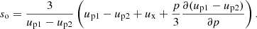
The ‘local’ spectral index s(p), that is, the local slope of the particle distribution f_o(p) at a given momentum p, is defined as

$$\begin{array}{c}\hfill s(p)=-\frac{\mathrm{d}ln{f}_{\mathrm{o}}}{\mathrm{d}lnp}.\end{array}$$(24)

Applying it to the function (23), we have

$$\begin{array}{c}\hfill s(p)=\frac{3u_{\mathrm{p}1}}{u_{\mathrm{p}1}-u_{\mathrm{p}2}}+\frac{\mathrm{d}ln(u_{\mathrm{p}1}-u_{\mathrm{p}2})}{\mathrm{d}lnp}.\end{array}$$(25)

This expression represents the spectral index for particles accelerated around the shock with a non-uniform spatial distribution of the flow speed u(x) upstream and downstream.

Let us introduce the effective compression factor that is ‘seen’ by particles with the momentum p (as shown in Fig. 2):

$$\begin{array}{c}\hfill {\sigma }_{\mathrm{eff}}(p)=\frac{u_{\mathrm{p}1}}{u_{\mathrm{p}2}}\approx \frac{u_1(x_{\mathrm{p}1})}{u_2(x_{\mathrm{p}2})}.\end{array}$$(26)

Fig. 2. Schematic representation of the structure of the flow velocity u(x) (solid line). The shock is located at the coordinate x = 0. The upstream profile of u(x) is shown for the case of the cosmic-ray-modified shock.

The spectral index for the cosmic-ray-modified shock (it is given by Eq. (8) in Blasi 2002) comes from (25) by assuming u₂ = const and therefore σ_eff = u_p1/u₂:

$$\begin{array}{c}\hfill s(p)=\frac{3{\sigma }_{\mathrm{eff}}}{{\sigma }_{\mathrm{eff}}-1}(1+\frac{1}{3}\frac{p}{{\sigma }_{\mathrm{eff}}}\frac{\mathrm{d}{\sigma }_{\mathrm{eff}}}{\mathrm{d}p}).\end{array}$$(27)

Equation (25) gives the classic test-particle index,

$$\begin{array}{c}\hfill s=\frac{3{\sigma }_{\mathrm{s}}}{{\sigma }_{\mathrm{s}}-1},\end{array}$$(28)

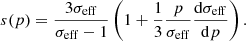
for u₁ = const and u₂ = const, namely by using the substitution σ_eff = σ_s = u₁/u₂. In the general case, where u₁(x)≠const and u₂(x)≠const, the contribution to s(p) from the first term in Eq. (25) is the same as for the unmodified shock (28) but with the effective compression factor σ_eff instead of σ_s. This contribution is modified somewhat by the second term in Eq. (25), which represents the ‘local’ (in the momentum space) slope of the difference u_p1 − u_p2. Below, we consider the effects of the spatially non-uniform u₂(x) on a few practical cases.

4.3. Benchmark problems

4.3.1. Test particles at the Sedov shock

We start from the acceleration of the test particles, that is, u₁ = const, at the adiabatic shock with the Sedov profile for u₂(x). For simplicity and clarity, we use the approximation by Taylor (1950) for the distribution of the flow velocity downstream of the shock, namely

$$\begin{array}{c}\hfill v(r)=v_2(R)r/R.\end{array}$$(29)

In the laboratory frame, the immediate post-shock value is v₂(R) = 3V/4, V is the shock speed, r is the distance from the explosion centre, and R is the shock radius. The accuracy of the approximation is better than 4% for > 0.7R (Fig. 1 in Petruk 2000). In the shock reference frame, the profile is

$$\begin{array}{c}\hfill u_2(x)=u_2(0)·(1+3x/R),\end{array}$$(30)

where u₂(0) = u₁/σ_s. We calculate u_p2 with the expression u_p2 ≈ u₂(x_p), which follows from the definition (15) and 𝒳₂(x) ≈ ℋ(x_p − x). In order to parametrise the dependence of the diffusion length x_p on p, we take

$$\begin{array}{c}\hfill x_{\mathrm{p}}(p)\propto \frac{D_2(p)}{u_2(0)},\end{array}$$(31)

where D is the spatially constant diffusion coefficient of the form D₂ ∝ p^α with α ≥ 0. Therefore,

$$\begin{array}{c}\hfill u_{\mathrm{p}2}=u_2(0)·(1+3{\overline{x}}_{\mathrm{p}}),{\overline{x}}_{\mathrm{p}}(p)={\overline{x}}_{\mathrm{pm}}·{(p/p_{\max })}^{\alpha },\end{array}$$(32)

where ${\overline{x}}_{\mathrm{pm}}\equiv x_{\mathrm{p}}(p_{\max })/R$ is the diffusion length for particles with the maximum momentum p_max normalised to R. In such a model, we can evaluate the spectral index analytically:

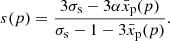$$\begin{array}{c}\hfill s(p)=\frac{3{\sigma }_{\mathrm{s}}-3\alpha {\overline{x}}_{\mathrm{p}}(p)}{{\sigma }_{\mathrm{s}}-1-3{\overline{x}}_{\mathrm{p}}(p)}.\end{array}$$(33)

In order to decipher the sensitivity of the problem to ${\overline{x}}_{\mathrm{pm}}$, we consider a few values of this parameter. We take these values for granted in the present section and explore their role further in Sect. 5.3.

In Fig. 3, we can see the local spectral index and the distribution function for the model we are considering. It is evident that the effect of the function u₂(x), which increases with x, leads to a higher s for higher p. (We note that in the observer frame, the flow speed v decreases downstream with distance from the shock.) This is because the effective compression factor σ_eff decreases with growing p (Fig. 2). Therefore, the momentum distribution function f_o(p) descends more rapidly than a common power law (Fig. 3).

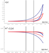Fig. 3. Local slopes s(p) and the distribution functions fo(p)/no for the unmodified Sedov shock. The parameters are ${\overline{x}}_{\mathrm{pm}}=0.1$ (blue lines), ${\overline{x}}_{\mathrm{pm}}=0.05$ (red lines), α = 1 (solid lines), α = 1/3 (dashed lines), and pmax = 104mpc. The classic value (for u2 = const) is s = 4 and is independent of p, α, and ${\overline{x}}_{\mathrm{pm}}$. Vertical lines: Left – energy of electrons for which the radio index is calculated in Fig. 6; right – protons with an energy of 240 GeV (see Sect. 5.2).

It is worth noting that the shapes of the particle distributions shown in Fig. 3 are only due to the plasma velocity gradient downstream of the shock. We applied only the sharp high-energy cutoff to the spectrum of particles ℋ(p_max − p), where ℋ(x) is the Heaviside step function. For comparison, the spectrum is just the power law up to the maximum momentum N(p) = K_p − sℋ(p_max − p) in the case of constant flow speed u₂(x) = const.

The classical test-particle index for the case of u₂ = const is s = 4. From Fig. 3, we observe that the local index s(p) for the Sedov velocity profile is close to this value for particles with low momenta p, that is, for the particles that are accelerated from small distances ${\overline{x}}_{\mathrm{p}}\approx 0$, where deviations of the flow velocity from u₂(0) are minor. The index s(p) increases with p for Sedov shock, and its maximum value happens for particles around p_max which are able to return to the shock from deeper downstream locations, that is, from around ${\overline{x}}_{\mathrm{pm}}$.

The effect described in the present paper is sensitive to α. For a fixed ${\overline{x}}_{\mathrm{pm}}$, the effect is more prominent for smaller α (Fig. 3) because particles with low momenta may return to the shock from deeper ${\overline{x}}_{\mathrm{p}}$ downstream regions.

Electrons in the magnetic field B = 10 μG emitting most of their energy through the synchrotron radiation at the radio frequency 5 GHz have an energy of 10 GeV. It is apparent from Fig. 3 that, at this energy, the spectral index differs by a few percent from the usual value. For example, the radio index is 0.52 for α = 1/3 and ${\overline{x}}_{\mathrm{pm}}=0.1$ instead of having the common value of 0.5. The differences are larger for smaller α. In the limit of a momentum-independent D (i.e. α = 0), the spectral index is also momentum independent. In such a toy model, its value depends on the distance x_p, which is the same for any p, as follows from the Eq. (32). Numerically, for the Sedov profile of u₂(x), the values are s = 4.4 for ${\overline{x}}_{\mathrm{pm}}=0.1$ and s = 4.2 for ${\overline{x}}_{\mathrm{pm}}=0.05$. The radio index at 5 GHz is 0.7 and 0.6, respectively.

4.3.2. Cosmic-ray-modified Sedov shock

Let us consider the acceleration of particles on the cosmic-ray-modified shock with the upstream profile u₁(x)≠const and the downstream distribution for u₂(x) given by Eq. (30), as in a Sedov SNR. The goal is to compare the spectra of particles with the case u₂(x) = const.

An intrinsic property of the non-linearity of the cosmic-ray modification of the shock is in the dependence of the plasma speed profile upstream of the shock u₁(x) on the particle distribution function f_o(p). If we have u₂(x) = const downstream of the shock, then the NLA solution of Blasi (2002) holds. In our problem, we should account for the spatial variation u₂(x) as well. We show above that the non-uniform profile u₂(x) affects the shape of the distribution function f_o(p). Therefore, the profile u₁(x) upstream will be differently modified by cosmic rays compared to the uniform u₂(x) distribution. In turn, this modified upstream profile affects f_o(p) as well.

We calculated the NLA solution for such a problem numerically in a self-consistent way by following the approach described by Blasi (2002), Blasi et al. (2005). Namely, we found the function u_p1(p) by iteratively solving the integro-differential equation, which depends on f_o(p), and accounts for the adiabatic evolution of the flow in the shock precursor, for the relation between the injection efficiency and the compression factor at the subshock, and – our addition – for the flow velocity structure downstream. The distribution function f_o(p) may then be found from Eq. (23). The iterations are repeated until the boundary condition u_p1(p_max) = u₀ is satisfied. We considered the following set of parameters: the Mach number ℳ_o = 100, the flow speed far upstream u₀ = 6.5 × 10⁸ cm s⁻¹, the maximum momentum p_max = 10⁴m_pc, and the injection efficiency η = 1.30 × 10⁻⁴. The red line on Fig. 4 shows the solution for u₂(x) = const, while the blue lines correspond to models with the velocity gradient downstream of the shock.

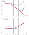Fig. 4. Plots of s(p) and fo(p)/no for the cosmic-ray-modified shock with u2(x) = const (red line) and with up2(p) given by the Eq. (32) with α = 1 (solid blue line), α = 1/3 (dashed blue line), ${\overline{x}}_{\mathrm{pm}}=0.1$, and pmax = 104mpc.

Qualitatively, we can understand the behaviour of the momentum distribution of accelerated particles from Fig. 2. In this scheme, we show a model of the cosmic-ray-modified shock (represented by the velocity profile in the x < 0 domain) with increasing function u₂(x) downstream (in the x > 0 domain). If we first consider the uniform u₂(x) (dashed grey horizontal line in Fig. 2), we can observe that particles with the lowest momenta ‘see’ the compression σ_s. Particles with larger momenta are affected by continuously higher compression σ_eff(p), which raises due to the velocity profile upstream. This is the main characteristic of the NLA solution shown by the red line in Fig. 4: the higher the effective compression, the lower the spectral index s and the harder the distribution f_o(p). However, the increasing function u₂(x) (solid line downstream in Fig. 2) progressively weakens this trend for higher momenta. As a result, the shape of the spectrum may be less concave compared to the pure NLA case or have a complex shape with an inflection point (blue lines in Fig. 4). In contrast, the decreasing u₂(x) causes stronger effective compression compared to the uniform u₂ downstream and strengthens the NLA concavity.

The effective compression factors are typically high in the NLA problem. They often lead to emission spectra with steep shapes, which are not observed in SNRs. To make σ_eff lower compared to the pure NLA case, Caprioli et al. (2009) considered the relative Alfenic speed v_A of the scattering centres (i.e. u + v_A instead of u in the diffusion–convection equation). Our model with a rising flow speed in the shock reference frame could be a natural way to lower σ_eff and make the spectrum flatter in circumstances where the cosmic-ray shock modification is an essential component.

It is worth noting that the injection efficiency we consider for Fig. 4 is not high, and the shock modification is not very strong. Indeed, the compression factor σ_tot ≡ u₀/u₂(0) is 5.434 for the red line, 5.359 for the blue solid line, and 4.897 for the blue dashed line. If the back-reaction of accelerated particles is higher –for example if σ_tot has a value of about 10 or more– then the upstream profile u₁(x) plays the dominating role in shaping f_o(p) compared to the effect from the downstream distribution u₂(x).

5. Discussion

We show in the previous section that the spatial variation of the flow speed downstream of the shock results in deviation of the momentum distribution of accelerated particles from the classic power law. The spectrum of emission produced by these particles should also be affected. This leads us to wonder whether this effect can be seen in any observables and what its strength might be. Let us look for an answer in the frame of the test-particle acceleration, that is, when assuming that u₁ = const.

5.1. Evolution of the radio index of young SNRs

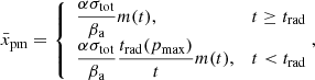
Previously, we explored magneto-hydrodynamic properties of young SNRs in examples of remnants from the three types of SNe (Petruk et al. 2021). Section 3 shows (see also the animation in Appendix A) that the temporal changes in the plasma velocity structure downstream of the shock u₂(x, t) are essential during the development of an SNR from the early stage (Chevalier 1982; Dwarkadas & Chevalier 1998) to the Sedov (1959) epoch. These changes may cause time variations in the momentum distribution of particles and consequently in the evolution of the radio index of SNRs.

Figure 5 shows the evolution of the effective compression factor for particles with the maximum momentum ${\sigma }_{\mathrm{eff}}(p_{\max })=u_1/u_2({\overline{x}}_{\mathrm{pm}})$ with ${\overline{x}}_{\mathrm{pm}}=0.1$ for three models of an SNR. The flow dynamics are different between the models. Specifically, the flow speed within ${\overline{x}}_{\mathrm{pm}}$ from the shock is almost the same in the SNIIP model, which is one of the representative cases for the DSA theory that assumes u₂(x) = const. On the other hand, the SNIa model demonstrates prominent changes in conditions for the shock particle acceleration during its evolution.

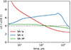Fig. 5. Effective compression factor $u_1/u_2({\overline{x}}_{\mathrm{pm}})$ with ${\overline{x}}_{\mathrm{pm}}=0.1$ for different ages. Models of SNRs are the same as in Sect. 3.

These differences may be present in the evolution of the radio index. To expose the effect, we approximate the profile of u₂(x, t) for the downstream region close to the shock using the linear function with a variable coefficient k:

$$\begin{array}{c}\hfill u_2(x,t)=u_2(0)·(1+k(t)x/R).\end{array}$$(34)

This approximation is justifiable by the shape of the u₂(x) profiles within the interval of x from zero to ∼0.1R (Fig. 1 and animation in Appendix A). The function u_p2(p) is then

$$\begin{array}{c}\hfill u_{\mathrm{p}2}(p)=u_2(0)·(1+k(t){\overline{x}}_{\mathrm{p}}(p))\end{array}$$(35)

instead of Eq. (32) and the local slope of the particle distribution is, instead of Eq. (33),

$$\begin{array}{c}\hfill s(p,t)=\frac{3{\sigma }_{\mathrm{s}}-k(t)\alpha {\overline{x}}_{\mathrm{p}}(p)}{{\sigma }_{\mathrm{s}}-1-k(t){\overline{x}}_{\mathrm{p}}(p)}.\end{array}$$(36)

The evolution of the radio index (s − 3)/2 calculated with this expression for s(p, t) is shown in Fig. 6. In the model SNIa, which displays the most prominent changes in the structure of the plasma speed (Fig. 5), the radio index varies from 0.46 to 0.54 over about 1000 yr (red solid line, s changes from 1.9 to 2.1 respectively). The range for the radio index variation could be even wider if particles probe deeper interiors of SNR during acceleration (i.e. when (x_pm > 0.1R or α smaller in the assumed dependence x_p(p), Eq. (32)), as shown by the dashed line in Fig. 6. It is also consistent with Fig. 3.

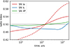Fig. 6. Evolution of the radio index at 5 GHz for the three models of SNRs and electrons with energy of 10 GeV (so, the magnetic field strength is 10 μG), pmax = 104mpc, ${\overline{x}}_{\mathrm{pm}}=0.1$, α = 1/3 (solid lines). The dashed line represents the same model as the solid line but with artificially taken α = 1/5.

We can conclude that the spectral index in the SNIa model is smaller than the value 0.5 up to SNR ages of ≈100 yr and higher at later times, as shown in Fig. 6. The reason is given by Eq. (36), which shows that the classic value s = 4 (and the radio index 0.5) corresponds to k = 0. Furthermore, this formula reveals that s could have a value of less than 4 when k < 0 (which happens when the flow velocity u₂ decreases with x, and thus the effective compression factor 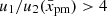$u_1/u_2({\overline{x}}_{\mathrm{pm}})>4$, as seen in Fig. 5) or above 4 when k > 0¹.

It is worth noting that the left vertical line in Fig. 3 corresponds to electrons that mostly determine the radio index shown in Fig. 6. We see that the deviation of their spectrum from the power law is minor. However, the deviation is more significant for particles with higher momenta, which emit X-rays and gamma-rays.

5.2. High-energy spectral break

A spectral feature is observed in the gamma-ray spectra of several SNRs that is attributed to a change in the slope of the proton spectrum, which is typically referred to as the broken power law. The change in the slope Δs ≈ 0.4 − 1 and should be added to proton spectrum models around the break momentum p_br, which has values from p_br = 10 GeV/c to p_br = 240 GeV/c to fit the observed spectra of some SNRs (e.g. Ackermann et al. 2013; H.E.S.S. Collaboration 2015, 2018).

Such a feature is also visible in radio (Loru et al. 2019) and microwave (Planck Collaboration XXXI 2016) spectra of SNRs, although it has roots in the momentum distribution of electrons.

Our results suggest that the particles accelerated at the shock with spatially variable flow velocity downstream have a momentum distribution with a smooth change of slope over a wide range of momenta. The radio-to-X-ray synchrotron spectrum is convex for evolved SNRs (when u₂(x) is an increasing function; Sect. 3), which could mimic the ‘break’ if not very sharp. Our calculations in Sect. 4.2 show that the slope changes between the particle energies 1 Gev and 300 Gev as Δs = 0.11 (from s = 4.02) or Δs = 0.30 (from s = 4.3) for Sedov shock and parameters $({\overline{x}}_{\mathrm{pm}},\alpha )$ from (0.1, 0.3) to (0.2, 0.1). Comparing these values of Δs with those required by observations, we see that the model could (at least partially) be responsible for the broken power law.

The difference in s(p) from the standard value s = 4 increases towards the maximum energy faster for larger ${\overline{x}}_{\mathrm{pm}}$ (i.e. the maximum distance from the shock the particles can be and still return to it), for higher values of k (i.e. how fast the flow speed u₂ grows with x), and for lower values of α (which is a measure of the extent to which the diffusion coefficient depends on the particle momentum).

This last point leads us to an important conclusion: the shape of the accelerated particle distribution in the momentum space is sensitive to the dependence of D on p if the flow speed is not spatially uniform. It is clear from Eq. (36) that the larger the absolute value of k, the higher the sensitivity.

In our model, the diffusion coefficient is a power-law function of the particle momentum D ∝ p^α across the whole range of p. As a result, the momentum spectrum of particles changes smoothly over the wide range of p. The observed spectral feature may reflect the change in the dependence of the diffusion coefficient on p around the break momentum p_br.

Figure 7 illustrates this concept, showing the same models as Fig. 3 but with a different diffusion coefficient for particles with the highest momenta. Namely, this coefficient is

$$\begin{array}{c}\hfill D(p)\propto \{\begin{array}{cc}{p}^{\alpha },\hfill & p<p_{\mathrm{br}}\hfill \\ p_{\mathrm{br}}^{\alpha }=\mathrm{const},\hfill & p\ge p_{\mathrm{br}}\hfill \end{array},\end{array}$$(37)

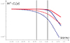Fig. 7. Distribution functions for the same cases as in Fig. 3. The only difference is the diffusion coefficient. It is the same as in Fig. 3 up to the momentum 0.1pmax and independent of p for higher momenta. Above 0.1pmax, the slopes s for the solid blue and red lines are 2.33 and 2.16, respectively. We note that all the lines will be straight horizontal up to pmax in the case of a uniform flow speed u2(x) = const.

with p_br = 0.1p_max. We see a sharp break around p ∼ 10³/mc in the solid lines representing the Bohm diffusion up to the break. The slope change is Δs = 0.33 for x_pm = 0.1 and Δs = 0.16 for x_pm = 0.05, meaning that it depends on the depth of the ‘zone’ downstream sampled by the accelerating particles. It is interesting to note that the slope s = 2.33 above p_br around the lower boundary of the values of s ≈ 2.3 − 2.6 is required to fit the observed gamma-ray spectra of some SNRs at photon energies of ≳1 TeV. The index s may even be higher in our model for appropriate x_pm and k.

We would like to emphasize that D(p) only influences s(p) if the flow speed is non-uniform, that is, in either the downstream or the upstream direction. If u₂(x) = const and u₁(x) = const, then particles of all momenta sample the same difference between u₁ and u₂ and therefore s is independent of p.

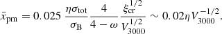
5.3. Evolution of the diffusion length

The effect we are considering depends on the spatial extent of the downstream region probed by particles accelerating at the shock. We expect the effect from the non-uniform flow velocity downstream of the shock to be noticeable in real SNRs if the diffusion length x_pm is higher than about 5% of the radius R.

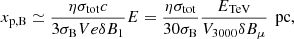
The Larmor radius of a proton or electron with energy E = E_TeV × 10¹² eV in the magnetic field B = B_μ × 10⁻⁶ G is r_L = 10⁻³E_TeV/B_μ pc. The length-scale downstream, which is involved in the formation of f_o(p), is of the order of the diffusion length x_p ≃ D₂/u₂. If diffusion is Bohm-like, then D_B = ηr_Lc/3 and

$$\begin{array}{c}\hfill x_{\mathrm{p}}\simeq \frac{4\eta c}{3V}{r}_{\mathrm{L}}.\end{array}$$(38)

The diffusion length could be up to x_p ∼ 10⁵r_L (for η = 100 and a slow shock V = 300 km s⁻¹). Under such extreme circumstances, even the radio-emitting electrons may effectively ‘feel’ the non-uniformity of the distribution of the flow speed, because the diffusion length may be up to x_p ∼ 0.1 pc for 10 GeV electrons in 10 μG magnetic field. Particles with energy E_max = 10 TeV may have x_p ∼ 0.1 pc in more common situations, such as in a magnetic field with a strength of 50 μG behind the shock with a speed of 6000 km s⁻¹ and η = 10.

In order to examine the sensitivity of the problem to the parameter 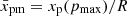${\overline{x}}_{\mathrm{pm}}=x_{\mathrm{p}}(p_{\max })/R$, we adopt fixed values for it and repeat the calculations in the previous sections. Let us examine how ${\overline{x}}_{\mathrm{pm}}$ evolves in the two alternative scenarios: the efficient acceleration with the Bohm diffusion and the test-particle case with the Kolmogorov diffusion coefficient.

The turbulent component of the magnetic field δB causes the scattering of particles. Equation (38) yields

$$\begin{array}{c}\hfill x_{\mathrm{p},\mathrm{B}}\simeq \frac{\eta {\sigma }_{\mathrm{tot}}c}{3{\sigma }_{\mathrm{B}}Ve\delta B_1}E=\frac{\eta {\sigma }_{\mathrm{tot}}}{30{\sigma }_{\mathrm{B}}}\frac{E_{\mathrm{TeV}}}{V_{3000}\delta B_{\mu }}\mathrm{pc},\end{array}$$(39)

where V₃₀₀₀ is the shock speed in units of 3000 km s⁻¹ and we used δB₂ = σ_BδB₁. It follows that the normalized diffusion length varies over time due to the expansion of the SNR, the evolution of p_max, and the magnetic field: ${\overline{x}}_{\mathrm{pm}}\propto p_{\max }/(VBR)$. We know the dependencies R(t) and V(t) for our SNR models from simulations.

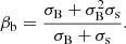
Under the efficient acceleration regime, we consider both the ordered B₁ and the random δB₁ components. At the young shocks, the Bell non-resonant instability operates with δB₁ > B₁. The saturated level of magnetic energy is approximately equal to the V/c fraction of energy E_cr stored in CRs (Bell 2004):

$$\begin{array}{c}\hfill \frac{\delta B_1^2}{4\pi }\simeq \frac{V}{c}{\xi }_{\mathrm{cr}}{\rho }_{\mathrm{o}}{V}^2,\end{array}$$(40)

where ξ_cr is the fraction of the kinetic energy transferred to CRs. When this δB₁ is less than the strength of the ordered field B₁, the resonant waves are responsible for the particle scatterings with (Amato & Blasi 2006)

$$\begin{array}{c}\hfill \frac{\delta B_1^2}{8\pi }\simeq \frac{v_{\mathrm{A}}}{V}{P}_{\mathrm{cr}},\end{array}$$(41)

where ${\mathit{v}}_{\mathrm{A}}=B_1/\sqrt{4\pi {\rho }_{\mathrm{o}}}$, P_cr = (γ_cr − 1)E_cr the CR pressure, γ_cr = 4/3 and δB₁/B₁ ≤ 1. The highest value of δB₁ for the resonant waves could be B₁. We assume δB₁ = B₁ in situations where these formulae give δB₁ < B₁ for the non-resonant and δB₁ > B₁ for the resonant, at the same time. Numerically, for the plasma with a mean particle mass in units of the proton mass μ = 0.609,

$$\begin{array}{c}\hfill \delta B_1=\{\begin{array}{cc}110{\xi }_{\mathrm{cr}}^{1/2}{n}_{\mathrm{o}}^{1/2}{V}_{3000}^{3/2}\mathrm{\mu }\mathrm{G},\hfill & \delta B_1>B_1\hfill \\ 27{\xi }_{\mathrm{cr}}^{1/2}{B}_{\mu }^{1/2}{n}_{\mathrm{o}}^{1/4}{V}_{3000}^{1/2}\mathrm{\mu }\mathrm{G},\hfill & \delta B_1<B_1\hfill \\ B_1\hfill & \mathrm{otherwise}.\hfill \end{array}\end{array}$$(42)

Figure 8 shows the variation of δB₁ with the SNR age in our models.

Fig. 8. Evolution of δB1 in three models of SNRs.

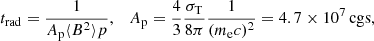
The mean acceleration time t_acc(p_max) could be estimated from a classic integral (Eq. (3.31) in Drury 1983) assuming D ∝ p^α, u₁ = V, u₂ = V/σ_tot:

$$\begin{array}{c}\hfill t_{\mathrm{acc}}(p_{\max })\simeq \frac{{\beta }_{\mathrm{a}}}{\alpha }\frac{D(p_{\max })}{V^2},{\beta }_{\mathrm{a}}=\frac{3{\sigma }_{\mathrm{tot}}(1+{\sigma }_{\mathrm{tot}}/{\sigma }_{\mathrm{B}})}{{\sigma }_{\mathrm{tot}}-1},\end{array}$$(43)

where β_a accounts for the fraction of time a particle spends upstream and downstream.

As expected, the acceleration time for diffusion with α < 1 is longer in 1/α times than in the case of the Bohm diffusion (α = 1), for example, for the Kolmogorov diffusion with α = 1/3, it is greater in 3 times.

One of three processes determines the maximum momentum of accelerated particles p_max. The condition t_acc(p_max) = t gives the maximum momentum limited by the SNR age. For the Bohm-like diffusion, we have

$$\begin{array}{c}\hfill p_{\max ,\mathrm{age},\mathrm{B}}=\frac{3e}{\eta {\beta }_{\mathrm{a}}}{\left(\frac{V}{c}\right)}^2\delta B_{1}t.\end{array}$$(44)

The synchrotron loss time, which is only applicable to electrons, is

$$\begin{array}{c}\hfill t_{\mathrm{rad}}=\frac{1}{A_{\mathrm{p}}⟨B^2⟩p},A_{\mathrm{p}}=\frac{4}{3}\frac{{\sigma }_{\mathrm{T}}}{8\pi }\frac{1}{{(m_{\mathrm{e}}c)}^2}=4.7\times {10}^7\mathrm{cgs},\end{array}$$(45)

with $\langle B^2\rangle ={\beta }_{\text{b}}{B}_{\text{rad}}^2$, where B_rad = max(δB₁, B₁) and β_b accounts for the time particles spend in the upstream and downstream (Reynolds 1998):

$$\begin{array}{c}\hfill {\beta }_{\mathrm{b}}=\frac{{\sigma }_{\mathrm{B}}+{\sigma }_{\mathrm{B}}^2{\sigma }_{\mathrm{s}}}{{\sigma }_{\mathrm{B}}+{\sigma }_{\mathrm{s}}}.\end{array}$$(46)

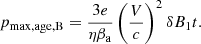
The equation t_acc(p_max) = t_rad(p_max) provides

$$\begin{array}{c}\hfill p_{\max ,\mathrm{rad},\mathrm{B}}={\left[\frac{3e}{\eta {\beta }_{\mathrm{a}}{\beta }_{\mathrm{b}}{A}_{\mathrm{p}}}{\left(\frac{V}{c}\right)}^2\frac{\delta B_1}{B_{\mathrm{rad}}^2}\right]}^{1/2}.\end{array}$$(47)

The third important time to account for is the time required for the growth of the Bell instability, which produces the magnetic field (Bell et al. 2013; Cardillo et al. 2015). In this case, the maximum momentum is estimated using equation (5) of Cristofari et al. (2020):

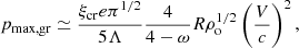$$\begin{array}{c}\hfill p_{\max ,\mathrm{gr}}\simeq \frac{{\xi }_{\mathrm{cr}}e{\pi }^{1/2}}{5\mathrm{\Lambda }}\frac{4}{4-\omega }R{\rho }_{\mathrm{o}}^{1/2}{\left(\frac{V}{c}\right)}^2,\end{array}$$(48)

where e is the electron charge, ω = −dlnn_o(R)/dlnR is the ambient density steepness (denoted m in Cardillo et al. 2015), and Λ ≈ 12 for p_max ∼ 100 TeV. This expression is valid for any type of diffusion and when the non-resonant δB₁ > B₁.

In an alternative scenario, we assume the test-particle acceleration and the Kolmogorov diffusion. We set the diffusion coefficient the same as the Bohm-like one at the particle energy E_o, that is, $D_{\mathrm{K}}=\eta c{E}_{\mathrm{o}}^{2/3}{E}^{1/3}/(3e\delta B)$. Then

$$\begin{array}{c}\hfill x_{\mathrm{p},\mathrm{K}}\simeq \frac{\eta {\sigma }_{\mathrm{tot}}c}{3{\sigma }_{\mathrm{B}}Ve\delta B_1}{E}_{\mathrm{o}}^{2/3}{E}^{1/3}=\frac{\eta {\sigma }_{\mathrm{tot}}}{30{\sigma }_{\mathrm{B}}}\frac{E_{\mathrm{o},\mathrm{TeV}}^{2/3}{E}_{\mathrm{TeV}}^{1/3}}{V_{3000}\delta B_{\mathrm{\mu }}}\mathrm{pc},\end{array}$$(49)

$$\begin{array}{c}\hfill p_{\max ,\mathrm{age},\mathrm{K}}={\left[\frac{e{c}^{2/3}}{\eta {\beta }_{\mathrm{a}}{E}_{\mathrm{o}}^{2/3}}{\left(\frac{V}{c}\right)}^2{B}_{1}t\right]}^3,\end{array}$$(50)

$$\begin{array}{c}\hfill p_{\max ,\mathrm{rad},\mathrm{K}}={\left[\frac{e{c}^{2/3}}{\eta {\beta }_{\mathrm{a}}{\beta }_{\mathrm{b}}{A}_{\mathrm{p}}{E}_{\mathrm{o}}^{2/3}}{\left(\frac{V}{c}\right)}^2\frac{\delta B_1}{B_{\mathrm{rad}}^2}\right]}^{3/4}.\end{array}$$(51)

The ‘test-particle’ relativistic protons do not amplify the magnetic field. Therefore, we do not account for p_max, gr in this scenario. The magnetic field strength for the diffusion coefficient and the radiative losses is the ordered one at the parallel shock, δB₁ = B_rad = B₁ = B₂.

The two scenarios for the evolution of the diffusion length ${\overline{x}}_{\mathrm{pm}}=x_{\mathrm{pm}}/R$ are summarised in Table 1. Figures 9 and 10 show the results of the calculations.

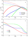Fig. 9. Evolution of the maximum momentum pmax (a) and the normalized diffusion length ${\overline{x}}_{\mathrm{pm}}$ (b) for particles with the maximum momentum in the test-particle acceleration scenario with Kolmogorov diffusion. Different colours show three of our models of SNRs. Line types represent the time-limited (dashed lines), loss-limited (dot-dashed lines) pmax, and the minimum of the two (solid lines). Lines for ${\overline{x}}_{\mathrm{pm}}$ correspond to the solid lines in the plot for the maximum momenta. pmax, rad < pmax, age from t = 1.3 kyr for the blue and t = 2.3 kyr for the green solid lines.

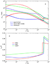Fig. 10. Same as in Fig. 9 but for the scenario of efficient acceleration. Dot-dashed lines represent pmax due to the Bell instability, which operates up to the time when the non-resonant δB1 > B1.

In the test-particle case, the maximum momentum in our models is limited predominantly by the age of the system (Fig. 9a). Interestingly, the three lines for ${\overline{x}}_{\mathrm{pm}}$ (Fig. 9b) are similar in shape to the evolution of the deceleration parameter m = Vt/R (Fig. 2 of Petruk et al. 2021). Indeed, if we express D from the relations t_acc = t or t_acc = t_rad and plug this into ${\overline{x}}_{\mathrm{pm}}={\sigma }_{\mathrm{tot}}D(p_{\max })/(RV)$, we get

$$\begin{array}{c}\hfill {\overline{x}}_{\mathrm{pm}}=\{\begin{array}{cc}{\displaystyle \frac{\alpha {\sigma }_{\mathrm{tot}}}{{\beta }_{\mathrm{a}}}m(t),}\hfill & t\ge t_{\mathrm{rad}}\hfill \\ {\displaystyle \frac{\alpha {\sigma }_{\mathrm{tot}}}{{\beta }_{\mathrm{a}}}\frac{t_{\mathrm{rad}}(p_{\max })}{t}m(t),}\hfill & t<t_{\mathrm{rad}}\hfill \end{array},\end{array}$$(52)

which is valid for diffusion of any type. If the age of the systems limits p_max, then the correlation ${\overline{x}}_{\mathrm{pm}}(t)\propto m(t)$ is clear. When the radiative losses limit the maximum energy of particles, then ${\overline{x}}_{\mathrm{pm}}$ also scales with parameters determining t_rad (Fig. 9b: blue line after t = 1.3 kyr and green line after t = 2.3 kyr). This could be essential in real SNRs when radiative losses limit p_max; for example when MF is amplified to high values. In this case, in a Sedov SNR for example, ${\overline{x}}_{\mathrm{pm}}\propto B^{-1/2}{t}^{8/5}$, which might provide a way to determine the properties of a magnetic field from the non-thermal spectra of SNRs. When p_max is age limited, the normalised diffusion length for particles with maximum momentum is determined solely by the shock compression and diffusion type (represented by α). In particular, for the Bohm-like (Kolmogorov) diffusion and unmodified shock, ${\overline{x}}_{\mathrm{pm}}\approx 20(6)\%$ of the SNR radius in young SNRs (when m ≈ 1) or ${\overline{x}}_{\mathrm{pm}}\approx 8(3)\%$ in SNRs at the Sedov stage (when m = 0.4).

In the scenario of efficient acceleration, p_max is limited by the growth rate of the Bell instability up to t ≈ 3 kyr (Fig. 10a, cf. Fig. 8). Eqs. (39), (40), and (48) then yield

$$\begin{array}{c}\hfill {\overline{x}}_{\mathrm{pm}}=0.025\frac{\eta {\sigma }_{\mathrm{tot}}}{{\sigma }_{\mathrm{B}}}\frac{4}{4-\omega }\frac{{\xi }_{\mathrm{cr}}^{1/2}}{V_{3000}^{1/2}}\sim 0.02\eta V_{3000}^{-1/2}.\end{array}$$(53)

The dependence on the shock speed is not strong, and the evolution of ${\overline{x}}_{\mathrm{pm}}$ is slow. Indeed, we see in Fig. 10b that the region downstream involved into the acceleration process is about 1 ÷ 3% of the radius when the Bell instability is effective. However, if the diffusion is Bohm-like with η = 2 ÷ 3, then ${\overline{x}}_{\mathrm{pm}}$ could reach 5% of the SNR radius. At times after ∼3 kyr, when the non-resonant instability is not effective in scattering the particles, then the SNR age limits the maximum momentum. At this stage, the diffusion length does not depend on η (Eqs. (41) and (44)) and may be up to ∼0.1R.

Thus, the downstream structure of the flow might have some influence on the shape of the non-thermal spectra of SNRs in both of the scenarios considered here. The effect is not sufficiently strong to modify the spectral indices in every SNR, but may do so in some cases under certain circumstances.

5.4. Limitations

The non-uniformity of the plasma speed behind the shock affects the cosmic-ray spectrum to a larger extent if particles can penetrate deeply downstream while accelerating at the shock. If so, they can probe a larger (for decreasing u₂(x)) difference between the upstream u_p1 and downstream u_p2 flow speeds and experience a higher burst in momentum: Δp ∝ u_p1 − u_p2. The distance from the shock depends on the properties of diffusion, x_p2 ≃ D/u₂. Therefore, in order for the effect from the downstream gradient of u₂ to be visible in the spectrum, the diffusion coefficient needs to be large. In our estimates, we considered x_p1 to be 5 ÷ 10% of the SNR radius R for the particles with the maximum momentum p_max = 10⁴m_pc ≈ 10 TeV/c. This corresponds to a diffusion coefficient for particles with such a momentum of D ∼ 0.1Ru₂ ∼ 3 × 10²⁵ cm² s⁻¹ (we used R ∼ 1 pc and u₂ ∼ 10³ km s⁻¹ for this estimate), which is well within typical values used in the literature. On the contrary, to be capable of providing the proton acceleration to energies beyond 100 TeV, the diffusion coefficient should be the smallest one, namely the Bohm coefficient D = r_Lc/3 in a magnetic field of a few hundred μG, which requires substantial magnetic field amplification. Under such conditions, the diffusion length for particles with energy E_max = 10 TeV is D₂/u₂ ≃ r_Lc/u₂ ∼ 0.01 pc, which is just ∼1% of R for particles with the maximum momentum. Of course, the variation of the plasma speed provided by the SNR hydrodynamics on such length scales downstream does not affect the shape of the CR spectrum. On the other hand, the length scale $x_{\text{p}}\propto D\propto p_{\text{max}}^{\alpha }$ also increases with the rise in maximum momentum.

In general, we expect the effect of the downstream velocity gradient to be prominent in SNRs – or in some local regions in SNRs – where the particle acceleration is not very efficient, that is, with a lower magnetic field and higher diffusion coefficient. In the present paper, the conditions studied therefore do not provide the highest E_max ∼ PeV energies. Instead, the maximum energy E_max ≈ 10 TeV we used in our examples is a value that can be reached in SNRs with a common interstellar magnetic field and without the fastest diffusion regime. It seems that the conditions for very efficient acceleration (amplified B of ∼ a few mG, the smallest Bohm diffusion coefficient), while crucial for the investigation of PeVatrons, are not widespread in SNRs. Such conditions could be expected locally, that is, present only in some small regions of the SNR shock surface. For an illustration of this point, we refer the reader to Fig. 4 of Long et al. (2003). The thinnest radial profile of the X-ray surface brightness in region A of SN1006 is due to the very fast radiative cooling of electrons in the high magnetic field. This profile provides evidence of effective acceleration with magnetic field amplification there. However, two other profiles B and C, which are close, are thicker (i.e. magnetic field is weaker in these regions). Therefore, the high magnetic strength inferred from the thinnest profile may not be generally attributed to the whole SNR. The less efficient particle acceleration could be in operation throughout other regions of the SNR shock surface.

Another important point is related to the dependence of the diffusion coefficient on the particle momentum; that is, the value of the index α. The effect of the gradient of u₂ could be more prominent with smaller particle momenta if the index α is less than unity (as in the Kolmogorov or Kraichnan diffusion coefficients), because x_p(p)∝x_p(p_max)p^α (see Figs. 3, 4, 7).

Interestingly, numerical studies of non-linear particle acceleration (where the kinetic particle equation is solved along with a system of hydrodynamic equations for the flow) by different groups (Kang & Jones 1995, 2007; Gieseler et al. 2000; Kang et al. 2002; Berezhko & Völk 1997, 2000; Zirakashvili & Aharonian 2010; Zirakashvili & Ptuskin 2012) used either the Bohm or the Bohm-like diffusion coefficient and did not find an appreciable impact of the downstream velocity gradient on the particle spectrum.

We find one report where the effect appears visible (though it is difficult to separate from the possible influence of other factors). Brose et al. (2020) numerically solved a system of equations for cosmic rays, magnetic turbulence, and plasma hydrodynamics in SNR. Their Fig. 2 compares the particle spectra for the Bohm diffusion (red lines) and the diffusion coefficient calculated self-consistently from the magnetic turbulence (green lines). In the latter case, the coefficient becomes Kolmogorov-like for most energies (Brose 2023, priv. commun.). The differences between the spectra shapes for α = 1 and α = 1/3 at the ages of 10 and 60 kyr are similar to ours in Fig. 3.

In summary, the effect of the non-uniform u₂(x) on the particle spectrum could be prominent in SNRs where adoption of Kolmogorov (α = 1/3) or Kraichnan diffusion (α = 1/2) in magnetic fields with standard strength B of a few tens of μG is acceptable, or in the case of a more efficient acceleration with the Bohm-like diffusion coefficient with η > 1.

In contrast, such values of α, B, and η are not compatible with the highest maximum energies of cosmic rays observed in several SNRs and are not consistent with a modern view of anisotropic cascade of MHD turbulence in the sources of highly efficient particle acceleration based on the Bohm diffusion and high values of amplified B.

6. Conclusions

The aim of the present study is to investigate the possible effect of a spatially variable distribution of the flow speed downstream of the shock on the momentum distribution of particles accelerated at the shock. To this end, we generalised the approach of Bell (1978b), which is an alternative way to describe the particle acceleration at the shock. This generalisation is itself of general academic interest.

We applied this generalised individual particle approach to the NLA solution of Blasi (2002), which assumes u₂(x) = const, and then to a more general problem with u₂(x)≠const. In order to cross-check our results, we derived in Appendix C the same general solution for f_o(p) by solving the kinetic equation.

The formula for the general solution (23) is similar to the known NLA solution. The difference consists in the substitution of the constant u₂ with u_p2(p).

In Sect. 3, we present profiles of the flow speed derived in numerical MHD simulations of remnants evolving after supernova explosions of different types. We demonstrate that the flow speed may vary prominently on the spatial scales involved in the acceleration of particles around the SNR shocks.

Then, we calculated the momentum spectra of particles for several practical cases to demonstrate the effect and its limitations. In these applications, we treat the problem by taking the formula (35) for the function u_p2(p).

Such a simplified description of u_p2(p) allows us to study the effect of a non-uniformity of the flow speed on the particle spectrum accelerated in the test-particle limits or the NLA regime (Sect. 4.3).

In Sect. 5, we suggest two cases where the phenomenon might affect – at least partially – some observed properties of SNRs. The overall effect may be visible from equation (36) written for the test-particle limit. If the flow speed in the frame of the shock rises with distance from the shock (i.e. k > 0, as in evolved SNRs) and particles with higher p reach larger x, then s grows with p. This results in a convex spectrum of particles. If the flow speed declines (k < 0), then s decreases and the spectrum is concave. The typical assumption of uniform flow downstream (k = 0) results in the classic formulae.

An important conclusion apparent from Eq. (36) is that the diffusion coefficient (represented by α in this formula) only directly affects the shape of f_o(p) if the flow speed is not uniform upstream and/or downstream. Diffusion properties of accelerating particles are important in shaping the f_o(p) because the diffusion coefficient determines the diffusive lengths for particles with different momenta. The momentum increase of a particle is sensitive to the differences in the flow velocities it probes u₁(x_p1)−u₂(x_p2). Therefore, the same speed profile u₂(x) affects the spectrum f_p(p) in a different way in models with distinct diffusion coefficients.

The effect of interest is rather sensitive to the diffusion properties of cosmic rays. Particles should diffuse far downstream to probe a hydrodynamic variation of u₂(x). Therefore, their diffusion length and diffusion coefficient should be high. As the acceleration of cosmic rays in SNRs to energies beyond 100 TeV is only likely to be achievable through the Bohm diffusion mechanism in an amplified magnetic field (where the diffusion length is therefore small), the significance of the downstream gradient of plasma velocity in SNRs capable of generating PeV cosmic rays can generally be disregarded.

Movie

Movie 1 (SNe_vx_animation) Access here

Acknowledgments

We acknowledge Elena Amato for useful discussions. OP acknowledges the OAPa grant number D.D.75/2022 funded by Direzione Scientifica of Istituto Nazionale di Astrofisica, Italy. The study was partially supported by the INAF mini-grant 1.05.23.04.04. This project has received funding through the MSCA4Ukraine project, which is funded by the European Union. Views and opinions expressed are however those of the author(s) only and do not necessarily reflect those of the European Union. Neither the European Union nor the MSCA4Ukraine Consortium as a whole nor any individual member institutions of the MSCA4Ukraine Consortium can be held responsible for them. We thank the Armed Forces of Ukraine for providing security to perform this work. This research used an HPC cluster at DESY, Germany, and the HPC system MEUSA at INAF-Osservatorio Astronomico di Palermo, Italy.

References

Appendix A: Evolution of the flow velocity downstream of the forward shock. Animation

The online animation shows the time development of the profiles of the flow speed v(r) in the observer reference frame (left) and u(x) in the shock reference frame (right) for the same models of SNRs as described in Sect. 3 and shown in Fig. 1, up to 10 000 yr. The horizontal axes represent r on the right plot and x = 1 − r/R on the left plot. Vertical axes are normalised to v₂(0) (left) and u₁(0) (right). The dashed line on each plot corresponds to the flow speed in the Sedov (1959) solution.

Appendix B: Probability of return

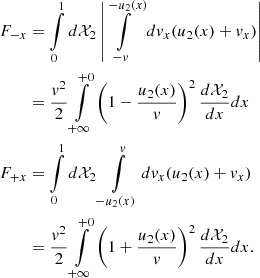
The probability of return P in one acceleration cycle is given by the ratio P = F_−x/F_+x where F_−x and F_+x are the fluxes of particles with momentum p in the negative and positive x-directions (Jones & Ellison 1991). In our case, the flow speed varies with x and we need to integrate over all places where the probability 𝒳₂(p,x) of finding particles with this momentum is above zero, i.e.

$$\begin{array}{cc}\hfill F_{-x}& ={\displaystyle \underset{0}{\overset{1}{\int }}}d{\mathcal{X}}_2\left|{\displaystyle \underset{-v}{\overset{-u_2(x)}{\int }}}d{v}_x(u_2(x)+v_x)\right|\hfill \\ \hfill & =\frac{v^2}{2}{\displaystyle \underset{+\infty }{\overset{+0}{\int }}}{(1-\frac{u_2(x)}{v})}^2\frac{d{\mathcal{X}}_2}{\mathit{dx}}dx\hfill \\ \hfill F_{+x}& ={\displaystyle \underset{0}{\overset{1}{\int }}}d{\mathcal{X}}_2{\displaystyle \underset{-u_2(x)}{\overset{v}{\int }}}d{v}_x(u_2(x)+v_x)\hfill \\ \hfill & =\frac{v^2}{2}{\displaystyle \underset{+\infty }{\overset{+0}{\int }}}{(1+\frac{u_2(x)}{v})}^2\frac{d{\mathcal{X}}_2}{\mathit{dx}}dx.\hfill \end{array}$$(B.1)

Transition to the rightmost equalities assumes that 𝒳₂ = 1 at x = +0 and 𝒳₂ = 0 for x = +∞. The simplified treatment of the probability in Sect. 4.1 may be recovered by taking approximately

$$\begin{array}{c}\hfill {\mathcal{X}}_2(x)=\mathcal{H}(x_{\mathrm{p}}-x),\end{array}$$(B.2)

and considering that dℋ(x_p − x)/dx = −δ(x − x_p). Then

$$\begin{array}{c}\hfill {\displaystyle P={\left(\frac{1-u_{\mathrm{p}2}/v}{1+u_{\mathrm{p}2}/v}\right)}^2,}\end{array}$$(B.3)

where u_p2 = u₂(x_p), as follows from approximation (B.2), and the definition

$$\begin{array}{c}\hfill u_{\mathrm{p}2}\equiv {\displaystyle {\int }_0^1}{u}_2(x)d{\mathcal{X}}_2=u_2(0)-{\displaystyle {\int }_{+\infty }^{+0}}{\mathcal{X}}_2(x)\frac{d{u}_2}{\mathit{dx}}dx.\end{array}$$(B.4)

In a more general treatment, we neglect the terms of the order (u₂/v)² in (B.1). Then, (1 ± u₂/v)² ≈ 1 ± 2u₂/v and, with the use of definition (B.4), the probability of return in one cycle becomes

$$\begin{array}{c}\hfill P=\frac{1-2u_{\mathrm{p}2}/v}{1+2u_{\mathrm{p}2}/v}.\end{array}$$(B.5)

In many cycles, we have the product of the probabilities for individual cycles. Decomposition of the logarithm of the product into the series to first order in u_p2/v yields equation (21).

Appendix C: Solution of the kinetic equation

This Appendix presents an alternative approach to deriving the expression (23) from the kinetic equation.

We consider the standard steady-state equation for the particle distribution function f(x, p):

$$\begin{array}{c}\hfill u\frac{\partial f}{\partial x}=\frac{\partial }{\partial x}\left[D\frac{\partial f}{\partial x}\right]+\frac{1}{3}\frac{\mathit{du}}{\mathit{dx}}p\frac{\partial f}{\partial p}+Q_{\mathrm{o}}(p)\delta (x),\end{array}$$(C.1)

together with the typical conditions: the flow speed is along the x axis, in the positive x direction; the shock is located at the coordinate x = 0; the velocity jump du/dx = (u₂ − u₁)δ(x) through the point x = 0; f(−0, p) = f(+0, p); f(x, p) = 0 at x = ±∞ and df/dx = 0 at x = −∞; the momentum part of the injection term

$$\begin{array}{c}\hfill {\displaystyle Q_{\mathrm{o}}(p)=\frac{\eta n_1{u}_1}{4\pi p^2}\delta (p-p_{\mathrm{o}}),}\end{array}$$(C.2)

where p_o is the injection momentum, η is the injection efficiency (the fraction of particles that start acceleration), p_o is the injection momentum, δ(x) is the delta-function, and the indices ‘1’ and ‘2’ mark upstream and downstream locations.

We consider the general situation where the flow speed profiles are not spatially constant: u₁(x)≠const, u₂(x)≠const. The approach to solving equation (C.1) is similar to solving the non-linear problem (Blasi 2002; Blasi et al. 2005); that is, we have to account for the spatial variations of the flow velocity.

The integration of the main equation (C.1) from −∞ to x = −0 results in

$$\begin{array}{c}\hfill {\left[D\frac{\partial f}{\partial x}\right]}_1=u_{\mathrm{p}1}{f}_{\mathrm{o}}-\frac{p}{3}\frac{\partial }{\partial p}{\displaystyle {\int }_{-\infty }^{-0}}f\frac{\mathit{du}}{\mathit{dx}}dx,\end{array}$$(C.3)

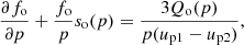
where f_o(p) is the distribution function at the shock. The integration of the equation (C.1) from x = −0 to x = +0 and from x = +0 to +∞ yields

$$\begin{array}{c}\hfill {\left[D\frac{\partial f}{\partial x}\right]}_2-{\left[D\frac{\partial f}{\partial x}\right]}_1+\frac{p}{3}\frac{\partial f_{\mathrm{o}}}{\partial p}(u_2-u_1)+Q_{\mathrm{o}}(p)=0\end{array}$$(C.4)

$$\begin{array}{c}\hfill {\left[D\frac{\partial f}{\partial x}\right]}_2=\frac{p}{3}\frac{\partial }{\partial p}{\displaystyle {\int }_{+0}^{+\infty }}f\frac{\mathit{du}}{\mathit{dx}}dx-{\displaystyle {\int }_{+0}^{+\infty }}u\frac{\partial f}{\partial x}dx-u_{\mathrm{x}}{f}_{\mathrm{o}}.\end{array}$$(C.5)

Integration of the last integral in (C.5) by parts transforms it to

$$\begin{array}{c}\hfill -{\displaystyle {\int }_{+0}^{+\infty }}u\frac{\partial f}{\partial x}dx=u_{\mathrm{p}2}{f}_{\mathrm{o}}.\end{array}$$(C.6)

We introduce the notations

$$\begin{array}{c}\hfill {\left[D\frac{\partial f}{\partial x}\right]}_{+\infty }=-u_3{f}_3\equiv -u_{\mathrm{x}}{f}_{\mathrm{o}},\end{array}$$(C.7)

where u₃ and f₃(p) are at the downstream infinity and u_x is an unknown function, as well as (cf. with equations (14)-(15))

$$\begin{array}{c}\hfill u_{\mathrm{p}1}(p)=u_1-{\displaystyle {\int }_{-\infty }^{-0}}\frac{f(x,p)}{f_{\mathrm{o}}(p)}\frac{\mathit{du}}{\mathit{dx}}dx,\end{array}$$(C.8)

$$\begin{array}{c}\hfill u_{\mathrm{p}2}(p)=u_2-{\displaystyle {\int }_{+\infty }^{+0}}\frac{f(x,p)}{f_{\mathrm{o}}(p)}\frac{\mathit{du}}{\mathit{dx}}dx.\end{array}$$(C.9)

With all these, equation (C.4) may be rewritten as the equation for the distribution function at the shock f_o(p):

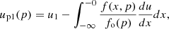
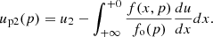
$$\begin{array}{c}\hfill \frac{\partial f_{\mathrm{o}}}{\partial p}+\frac{f_{\mathrm{o}}}{p}{s}_{\mathrm{o}}(p)=\frac{3Q_{\mathrm{o}}(p)}{p(u_{\mathrm{p}1}-u_{\mathrm{p}2})},\end{array}$$(C.10)

$$\begin{array}{c}\hfill s_{\mathrm{o}}=\frac{3}{u_{\mathrm{p}1}-u_{\mathrm{p}2}}(u_{\mathrm{p}1}-u_{\mathrm{p}2}+u_{\mathrm{x}}+\frac{p}{3}\frac{\partial (u_{\mathrm{p}1}-u_{\mathrm{p}2})}{\partial p}).\end{array}$$(C.11)

The solution of this equation is

$$\begin{array}{c}\hfill f_{\mathrm{o}}(p)=\frac{\eta n_1}{4\pi p_{\mathrm{o}}^3}\frac{3u_1}{u_{\mathrm{p}1}-u_{\mathrm{p}2}}exp[-{\displaystyle {\int }_{p_{\mathrm{o}}}^p}\frac{3(u_{\mathrm{p}1}-u_{\mathrm{p}2}+u_{\mathrm{x}})}{u_{\mathrm{p}1}-u_{\mathrm{p}2}}\frac{d{p^{\prime }}^{}}{{p^{\prime }}^{}}].\end{array}$$(C.12)

The unknown function u_x should be u_x = u_p2 in order (i) to match the expression (23) derived in the frame of the approach of Bell, (ii) to give the Blasi (2002) solution with u₂ = const (cf. eq.(8) in Blasi et al. 2005), and (iii) to yield the classic test-particle solution f_o ∝ p^{−3u₁/(u₁ − u₂)} with u₁ = const and u₂ = const (then u_p1 = u₁ and u_p2 = u₂).

Strictly speaking, u_x in the solution (C.12) is u_x = u₃f₃(p)/f_o(p) (see eq. C.7). The equality u_x = u_p2 is valid in the case (i) above at least to the level of approximation for the spatial ‘part’ of the distribution function f₂(x, p) adopted in the present paper, i.e. f₂(x,p) ≈ f_o(p)ℋ(x_p − x). Indeed, let us consider some point x_p′ downstream. The advected flux of particles with momentum p′ from this point toward x > x_p′ is proportional to u₂(x_p′)f_o(p′). The flux conservation gives u₃f₃(p′) = u₂(x_p′)f_o(p′). Similarly, u₃f₃(p″) = u₂(x_p″)f_o(p″) for particles with another momentum p″, and so on. Therefore, u₃f₃(p) = u₂(x_p)f_o(p) holds for any momentum p of relativistic particles. From the definition (15) and 𝒳₂(x) = ℋ(x_p − x), we have that u₂(x_p) = u_p2. Thus, u₃f₃(p)/f_o(p) = u_p2 and, from (C.7), u_x = u_p2.

It would be desirable in the future to determine the distribution f₃(p) from more general considerations. This task is related to the problem of distinguishing between the distribution functions of two populations of particles, namely those that continue to participate in acceleration and those advected downstream. Nevertheless, the exact evolution of particles advected toward the downstream infinity seems unimportant in the determination of the distribution function at the shock because they are ‘removed’ from the accelerator. Therefore, one may set up the boundary condition (C.7) as u₃f₃(p) = u_p2f_o a priori.

All Tables

All Figures

Fig. 1. Profiles of the flow velocity v(r) in the observer reference frame (left) and u(x) in the shock reference frame (right) for the three models of SNRs. Upper row: Three SNe models at 500 yr. Lower row: SNIa model at the ages 20, 200, and 1000 yr. On the plots to the left, the explosion centre is at r = 0 with the zero velocity v there. On the plots to the right, the horizontal axes display x = 1 − r/R. Therefore, negative values correspond to the upstream region, whereas positive values correspond to the downstream region. The centre of the explosion on the right-hand side plots is at x = 1, and the velocity u at this point is equal to the upstream velocity u1. We conducted the numerical simulations for the unmodified shocks, and therefore u is spatially constant upstream. The dashed line represents the velocity profile from the Sedov (1959) solution.

In the text

	Fig. 2. Schematic representation of the structure of the flow velocity u(x) (solid line). The shock is located at the coordinate x = 0. The upstream profile of u(x) is shown for the case of the cosmic-ray-modified shock.
In the text

Fig. 3. Local slopes s(p) and the distribution functions fo(p)/no for the unmodified Sedov shock. The parameters are ${\overline{x}}_{\mathrm{pm}}=0.1$ (blue lines), ${\overline{x}}_{\mathrm{pm}}=0.05$ (red lines), α = 1 (solid lines), α = 1/3 (dashed lines), and pmax = 104mpc. The classic value (for u2 = const) is s = 4 and is independent of p, α, and ${\overline{x}}_{\mathrm{pm}}$. Vertical lines: Left – energy of electrons for which the radio index is calculated in Fig. 6; right – protons with an energy of 240 GeV (see Sect. 5.2).

In the text

	Fig. 4. Plots of s(p) and fo(p)/no for the cosmic-ray-modified shock with u2(x) = const (red line) and with up2(p) given by the Eq. (32) with α = 1 (solid blue line), α = 1/3 (dashed blue line), ${\overline{x}}_{\mathrm{pm}}=0.1$, and pmax = 104mpc.
In the text

	Fig. 5. Effective compression factor $u_1/u_2({\overline{x}}_{\mathrm{pm}})$ with ${\overline{x}}_{\mathrm{pm}}=0.1$ for different ages. Models of SNRs are the same as in Sect. 3.
In the text

	Fig. 6. Evolution of the radio index at 5 GHz for the three models of SNRs and electrons with energy of 10 GeV (so, the magnetic field strength is 10 μG), pmax = 104mpc, ${\overline{x}}_{\mathrm{pm}}=0.1$, α = 1/3 (solid lines). The dashed line represents the same model as the solid line but with artificially taken α = 1/5.
In the text

Fig. 7. Distribution functions for the same cases as in Fig. 3. The only difference is the diffusion coefficient. It is the same as in Fig. 3 up to the momentum 0.1pmax and independent of p for higher momenta. Above 0.1pmax, the slopes s for the solid blue and red lines are 2.33 and 2.16, respectively. We note that all the lines will be straight horizontal up to pmax in the case of a uniform flow speed u2(x) = const.

In the text

	Fig. 8. Evolution of δB1 in three models of SNRs.
In the text

Fig. 9. Evolution of the maximum momentum pmax (a) and the normalized diffusion length ${\overline{x}}_{\mathrm{pm}}$ (b) for particles with the maximum momentum in the test-particle acceleration scenario with Kolmogorov diffusion. Different colours show three of our models of SNRs. Line types represent the time-limited (dashed lines), loss-limited (dot-dashed lines) pmax, and the minimum of the two (solid lines). Lines for ${\overline{x}}_{\mathrm{pm}}$ correspond to the solid lines in the plot for the maximum momenta. pmax, rad < pmax, age from t = 1.3 kyr for the blue and t = 2.3 kyr for the green solid lines.

In the text

References

- Ackermann, M., Ajello, M., Allafort, A., et al. 2013, Science, 339, 807 [NASA ADS] [CrossRef] [Google Scholar]
- Amato, E., & Blasi, P. 2005, MNRAS, 364, L76 [NASA ADS] [Google Scholar]
- Amato, E., & Blasi, P. 2006, MNRAS, 371, 1251 [NASA ADS] [CrossRef] [Google Scholar]
- Axford, W. I., Leer, E., & Skadron, G. 1977, Int. Cosmic Ray Conf., 11, 132 [Google Scholar]
- Bell, A. R. 1978a, MNRAS, 182, 147 [Google Scholar]
- Bell, A. R. 1978b, MNRAS, 182, 443 [Google Scholar]
- Bell, A. R. 2004, MNRAS, 353, 550 [Google Scholar]
- Bell, A. R., Schure, K. M., Reville, B., & Giacinti, G. 2013, MNRAS, 431, 415 [Google Scholar]
- Berezhko, E. G., & Völk, H. J. 1997, Astropart. Phys., 7, 183 [NASA ADS] [CrossRef] [Google Scholar]
- Berezhko, E. G., & Völk, H. J. 2000, A&A, 357, 283 [NASA ADS] [Google Scholar]
- Blandford, R. D., & Ostriker, J. P. 1978, ApJ, 221, L29 [Google Scholar]
- Blasi, P. 2002, Astropart. Phys., 16, 429 [NASA ADS] [CrossRef] [Google Scholar]
- Blasi, P., Gabici, S., & Vannoni, G. 2005, MNRAS, 361, 907 [NASA ADS] [CrossRef] [Google Scholar]
- Bogdan, T. J., & Volk, H. J. 1983, A&A, 122, 129 [NASA ADS] [Google Scholar]
- Brose, R., Pohl, M., Sushch, I., Petruk, O., & Kuzyo, T. 2020, A&A, 634, A59 [EDP Sciences] [Google Scholar]
- Caprioli, D., Blasi, P., Amato, E., & Vietri, M. 2009, MNRAS, 395, 895 [Google Scholar]
- Caprioli, D., Amato, E., & Blasi, P. 2010, Astropart. Phys., 33, 307 [NASA ADS] [CrossRef] [Google Scholar]
- Cardillo, M., Amato, E., & Blasi, P. 2015, Astropart. Phys., 69, 1 [Google Scholar]
- Chevalier, R. A. 1982, ApJ, 258, 790 [NASA ADS] [CrossRef] [Google Scholar]
- Cristofari, P., Blasi, P., & Amato, E. 2020, Astropart. Phys., 123, 102492 [Google Scholar]
- Drury, L. O. 1983, Rep. Prog. Phys., 46, 973 [Google Scholar]
- Dwarkadas, V. V., & Chevalier, R. A. 1998, ApJ, 497, 807 [NASA ADS] [CrossRef] [Google Scholar]
- Ferrand, G., Warren, D. C., Ono, M., et al. 2019, ApJ, 877, 136 [Google Scholar]
- Ferrand, G., Warren, D. C., Ono, M., et al. 2021, ApJ, 906, 93 [NASA ADS] [CrossRef] [Google Scholar]
- Gabler, M., Wongwathanarat, A., & Janka, H.-T. 2021, MNRAS, 502, 3264 [CrossRef] [Google Scholar]
- Gieseler, U. D. J., Jones, T. W., & Kang, H. 2000, A&A, 364, 911 [NASA ADS] [Google Scholar]
- H.E.S.S. Collaboration (Abramowski, A., et al.) 2015, A&A, 574, A100 [CrossRef] [EDP Sciences] [Google Scholar]
- H.E.S.S. Collaboration (Abdalla, H., et al.) 2018, A&A, 612, A5 [NASA ADS] [CrossRef] [EDP Sciences] [Google Scholar]
- Jones, F. C., & Ellison, D. C. 1991, Space Sci. Rev., 58, 259 [Google Scholar]
- Kang, H., & Jones, T. W. 1995, ApJ, 447, 944 [NASA ADS] [CrossRef] [Google Scholar]
- Kang, H., & Jones, T. W. 2007, Astropart. Phys., 28, 232 [NASA ADS] [CrossRef] [Google Scholar]
- Kang, H., Jones, T. W., & Gieseler, U. D. J. 2002, ApJ, 579, 337 [CrossRef] [Google Scholar]
- Krymskii, G. 1977, Akademiia Nauk SSSR Doklady, 234, 1306 [NASA ADS] [Google Scholar]
- Long, K. S., Reynolds, S. P., Raymond, J. C., et al. 2003, ApJ, 586, 1162 [Google Scholar]
- Loru, S., Pellizzoni, A., Egron, E., et al. 2019, MNRAS, 482, 3857 [CrossRef] [Google Scholar]
- Malkov, M. A., & Drury, L. O. 2001, Rep. Prog. Phys., 64, 429 [NASA ADS] [CrossRef] [Google Scholar]
- Mignone, A., Bodo, G., Massaglia, S., et al. 2007, ApJS, 170, 228 [Google Scholar]
- Mignone, A., Zanni, C., Tzeferacos, P., et al. 2012, ApJS, 198, 7 [Google Scholar]
- Orlando, S., Miceli, M., Pumo, M. L., & Bocchino, F. 2015, ApJ, 810, 168 [NASA ADS] [CrossRef] [Google Scholar]
- Patnaude, D. J., Lee, S.-H., Slane, P. O., et al. 2015, ApJ, 803, 101 [NASA ADS] [CrossRef] [Google Scholar]
- Petruk, O. 2000, A&A, 357, 686 [NASA ADS] [Google Scholar]
- Petruk, O., Kuzyo, T., Orlando, S., Pohl, M., & Brose, R. 2021, MNRAS, 505, 755 [NASA ADS] [CrossRef] [Google Scholar]
- Planck Collaboration XXXI. 2016, A&A, 586, A134 [NASA ADS] [CrossRef] [EDP Sciences] [Google Scholar]
- Reynolds, S. P. 1998, ApJ, 493, 375 [NASA ADS] [CrossRef] [Google Scholar]
- Sedov, L. I. 1959, Similarity and Dimensional Methods in Mechanics (New York: Academic Press Inc.) [Google Scholar]
- Taylor, G. 1950, Proc. Royal Soc. London Ser. A, 201, 159 [NASA ADS] [Google Scholar]
- Telezhinsky, I., Dwarkadas, V. V., & Pohl, M. 2012, Astropart. Phys., 35, 300 [NASA ADS] [CrossRef] [Google Scholar]
- Telezhinsky, I., Dwarkadas, V. V., & Pohl, M. 2013, A&A, 552, A102 [NASA ADS] [CrossRef] [EDP Sciences] [Google Scholar]
- Zirakashvili, V. N., & Aharonian, F. A. 2010, ApJ, 708, 965 [NASA ADS] [CrossRef] [Google Scholar]
- Zirakashvili, V. N., & Ptuskin, V. S. 2012, Astropart. Phys., 39, 12 [Google Scholar]