| Issue |
A&A
Volume 686, June 2024
|
|
|---|---|---|
| Article Number | A242 | |
| Number of page(s) | 18 | |
| Section | Astrophysical processes | |
| DOI | https://doi.org/10.1051/0004-6361/202348817 | |
| Published online | 18 June 2024 | |
Cygnus OB2 as a test case for particle acceleration in young massive star clusters
1
INAF – Osservatorio Astrofisico di Arcetri, Largo Enrico Fermi 5, Firenze, Italy
e-mail: stefano.menchiari@inaf.it
2
Università degli studi di Siena, Dipartimento di scienze fisiche della terra e dell’ambiente, Via Roma 56, 53100 Siena, Italy
Received:
1
December
2023
Accepted:
3
March
2024
In this paper, we focus on the scientific case of Cygnus OB2, a young massive star cluster (YMSC) located in the northern sky towards the Cygnus X star-forming complex. We consider a model that assumes cosmic-ray acceleration occurring only at the termination shock of the collective wind of the YMSC and address the question of whether or not, and under what hypotheses, hadronic emission by the accelerated particles can account for the observations of Cygnus OB2 obtained by Fermi-LAT and HAWC. To this end, we carefully review the available information on this source, also confronting different estimates of the relevant parameters with ad hoc developed simulations. Once other model parameters are fixed, the spectral and spatial properties of the emission are found to be very sensitive to the unknown properties of the turbulent magnetic field. Comparison with the data shows that our suggested scenario is incompatible with Kolmogorov turbulence. Assuming Kraichnan- or Bohm-type turbulence spectra, the model accounts well for the very high energy (VHE) data, but fails to reproduce the centrally peaked morphology observed by Fermi-LAT, suggesting that additional effects might be important for lower energy γ-ray emission. We discuss how additional progress can be made with more detailed and extended knowledge of the spectral and morphological properties of the emission.
Key words: acceleration of particles / radiation mechanisms: non-thermal / ISM: bubbles / cosmic rays / gamma rays: ISM / ISM: individual objects: Cygnus OB2
© The Authors 2024
 Open Access article, published by EDP Sciences, under the terms of the Creative Commons Attribution License (https://creativecommons.org/licenses/by/4.0), which permits unrestricted use, distribution, and reproduction in any medium, provided the original work is properly cited.
This article is published in open access under the Subscribe to Open model. Subscribe to A&A to support open access publication.
1. Introduction
The origin of cosmic rays (CRs) is a century-long enigma that still lacks a final solution. There is a general consensus that supernova remnants (SNRs) are the main factories of Galactic CRs, which is based on both theoretical arguments and observational evidence. From a theoretical point of view, SNRs are capable of accelerating particles through the diffusive shock acceleration process (Drury 1983) that occurs at the shock front driven by the supersonic motion of the supernova ejecta as they expand in the interstellar medium (ISM). In addition, assuming that 10% of the kinetic energy released in a supernova explosion goes into accelerating particles, a supernova rate of approximately two explosions per century is sufficient to sustain the measured CR luminosity (Baade & Zwicky 1934). From the observational side, X-ray observations of several SNRs have confirmed the presence of relativistic electrons with inferred energies of up to tens of TeV, the maximum allowed by efficient radiation-loss-limited acceleration at the SNR shock (Koyama et al. 1995; Reynolds 2008; Helder et al. 2012), while the detection of the pion bump at ∼1 GeV is proof of the hadronic nature of the γ-ray emission from several SNRs (see Funk 2017, for a review).
However, the SNR paradigm still fails to properly account for some fundamental properties of CRs. The first issue concerns their composition: CR measurements at Earth have revealed some anomalous isotopic ratios, the most noticeable being that of 22Ne/20Ne, which is found to be ≃5.3 times higher than the solar value (Wiedenbeck & Greiner 1981; Binns et al. 2008). An additional problem is the maximum energy attainable at SNR shocks. To explain the ‘knee’ in the CR spectrum, protons need to be accelerated up to at least ∼1 PeV, while observations suggest that SNRs only achieve much lower energies; that is, lower by at least one order of magnitude. Such observations are indeed in agreement with theoretical models, which predict maximum energies of up to ∼100 TeV for typical SNRs (Bell et al. 2013; Cardillo et al. 2015), unless extreme conditions are assumed (Cristofari et al. 2022).
One possible solution to the above-mentioned problems is that, in addition to SNRs, other classes of sources may be contributing to the production of Galactic CRs. In particular, the chemical composition requires that at least a fraction of CRs should come from the acceleration of massive star wind material (Prantzos 2012). Since the 80s, stellar winds have been proposed as possible CR factories (Casse & Paul 1980; Cesarsky & Montmerle 1983), especially in the context of young massive star clusters (YMSCs). The consensus around this hypothesis has rapidly grown in the last decade, as several experiments have detected both high-energy and very-high-energy (VHE) extended γ-ray emission in coincidence with various YMSCs, such as Cygnus OB2 (Ackermann et al. 2011; Bartoli et al. 2014; Abeysekara et al. 2021; Astiasarain et al. 2023), Westerlund 1 (Abramowski et al. 2012; Aharonian et al. 2022), and Westerlund 2 (Yang et al. 2018), NGC 3603 (Saha et al. 2020). The most common hypothesis regarding the origin of the energy powering these objects is that it results from an accumulation of the powerful winds blown by the hundreds of massive stars hosted in the clusters. CR acceleration could potentially be achieved in different ways. One possibility is that CRs are accelerated inside the cluster core, where particle energies are increased by multiple crossings of the shocks induced by wind–wind collisions (Reimer et al. 2006), or by efficient scattering on the magnetic turbulence caused by such collisions (Bykov et al. 2020). On the other hand, in the case of compact YMSCs, the winds from massive stars can combine to create a collective cluster wind. In this case, particle acceleration can result from diffusive shock acceleration at the wind termination shock (TS; Morlino et al. 2021). In clusters older than ∼5 Myr, multiple supernova explosions are expected to be the dominant energy source for CR production (Vieu et al. 2022a).
Young massive star clusters and their possible contribution of CRs could indeed be the missing piece of the CR origin puzzle, because these sources can potentially account for the CR properties that the SNR paradigm fails to explain: the composition of the YMSC wind material can in principle account for the anomalous 22Ne to 20Ne ratio (Gupta et al. 2020; Tatischeff et al. 2021); in addition, the maximum achievable energy in these systems can be as high as a few PeV. In the case of acceleration taking place at the wind TS, as shown by Morlino et al. (2021), depending on the plasma turbulence spectrum, CRs can smoothly reach PeV energies if ∼10% of the YMSC wind luminosity ends in the turbulent magnetic field and particle diffusion is close to Bohm-like. An even higher energy could be reached by SNR shocks propagating inside the wind-blown bubble, where the turbulence level has been preliminarily enhanced by the same stellar winds (Vieu et al. 2022b). It is important to stress that the conditions needed to reach such high energies in YMSCs have not yet been verified: in particular the particle acceleration efficiency and the properties of magnetic turbulence in these systems are currently unknown. Indeed, the wind-blown bubble is a very complex system, and a proper theoretical modelling requires numerical simulations able to take into account several physical processes (see e.g. Lancaster et al. 2021). In terms of observations, on the other hand, the most direct diagnostic of the relevant physical conditions is offered by spectro-morphological analysis of the emission in the γ-ray range, where radiation of hadronic origin may be detected.
In the present paper, we consider the YMSC Cygnus OB2, and try to model – under the assumption of pure hadronic processes – the γ-ray emission detected by several experiments. We assume that particles are accelerated at the collective wind TS using the model developed by Morlino et al. (2021). A similar analysis is presented by Blasi & Morlino (2023). The present paper complements this latter work in several ways. Firstly, we carefully model the local gas distribution as inferred by the measured column density. Secondly, we illustrate the method used to estimate the total cluster’s wind power, a parameter that is common to our work and that of Blasi & Morlino (2023), the estimation of which is usually treated in a very cursory manner. Finally, rather than fixing a priori a model for particle transport, we consider the magnetic turbulence as an unknown and attempt to fit the γ-ray emission from the Cygnus OB2 region (often referred to as the Cygnus ‘cocoon’) with different underlying turbulence models. More specifically, we consider all of the most common models of magnetic turbulence in astrophysics, namely Kolmogorov’s, Kraichnan’s and Bohm’s, and use γ-ray observations to determine which is the most viable.
The paper is structured as follows: in Sect. 2, we describe the general properties of the Cygnus OB2 star cluster. In Sect. 3, we present the properties of the expected CR distribution close to a YMSC. In Sect. 4, we calculate its associated γ-ray emission and we compare it with available data in Sect. 5. A detailed discussion of the analysis is provided in Sect. 6 and we draw our conclusions in Sect. 7.
2. The Cygnus OB2 association and its surroundings
Cygnus OB2 (Cyg OB2) is one of the most massive and compact OB associations in the Milky Way (l ≃ 80.22°, b ≃ 0.79°) harbouring hundreds, possibly thousands, of massive stars. The first study of its population was carried out by Reddish et al. (1966), who inferred a total of 400–3000 OB stars, by counting them on the Palomar Sky Survey plates. Knödlseder (2000) found a compatible result using near-infrared images, with an estimated total population of 2600 ± 400 OB stars, among which 120 ± 20 O-type stars. Such numbers are probably overestimated due to the problematic background subtraction and the highly patchy extinction pattern towards the association: in a more recent work, which better accounted for these issues, Wright et al. (2010) estimated a total content of ∼1200 OB stars, with ∼75 O-type stars.
In terms of spatial distribution, the cluster is compact, and the stars show a centrally peaked radial profile, with a high stellar density at the center of the association, similar to the YMSCs observed in the Large Magellanic Cloud (Knödlseder 2000). A large fraction of the stars is enclosed in a region of radius ∼14 pc. A recent census of this central core has revealed the presence of 3 Wolf-Rayet stars and 166 OB stars, among which 52 are classified as O-type (Wright et al. 2015).
Several different estimates have been made of the age of Cyg OB2. The presence of O-type dwarf stars and high-luminosity blue supergiants in the sample of 85 OB stars selected by Hanson (2003) suggests that Cyg OB2 should not be older than a few million years, with a most likely age of 2 ± 1 Myr. On the other hand, a study of the population of A-type stars indicated the presence of a group of 5–7 Myr old stars, located mainly in the southern part of the association (Drew et al. 2008). In parallel, X-ray analysis of low-mass stars seems to point to an age of 3–5 Myr (Wright et al. 2010). Wright et al. (2015) found a typical age of 2–3 Myr and 4–5 Myr by applying, respectively, non-rotating and rotating evolutionary stellar models to a selected sample of 169 OB stars. All these results might be reconciled in a scenario of continuous star formation activity starting ∼7 Myr ago and extending to ∼1 Myr ago, with a possible peak of star formation around 4–5 Myr ago. This is also compatible with the results found by Comerón & Pasquali (2012), who suggested a continuous star-forming activity in the region for the last 10 Myr.
The distance of Cyg OB2 is a subject of debate. Right after the discovery of the association, Johnson & Morgan (1954) inferred a distance of ∼1500 pc using spectroscopic observations of 11 stars. In the first comprehensive investigation of the Cyg OB2 population, Reddish et al. (1966) estimated a distance of 2100 pc. In the early 90s, independent studies, based on the method of spectroscopic parallax, evaluated a distance of ∼1700 pc (Torres-Dodgen et al. 1991; Massey & Thompson 1991). Currently, the most commonly adopted value is the one determined by Hanson (2003), who calculated a distance of 1400 ± 80 pc after a detailed analysis of the absolute magnitude and extinction of 14 OB stars. This estimate is compatible with the position of some molecular clouds in the Cygnus-X region, whose distance has been calculated using maser parallaxes (Rygl et al. 2012). Moreover, the value is also in agreement with the recent result of 1330 ± 60 pc based on the parallaxes of some eclipsing binaries (Kiminki et al. 2015). Finally, Gaia’s parallaxes from the second data release (Berlanas et al. 2019) point out that the association might be composed of two main subgroups, the first located at a distance of ∼1350 pc and the second at ∼1755 ± 320 pc. In this work, we assume a distance of 1400 pc in order to retain consistency with Wright et al. (2015), who used this distance to estimate the spectral types of stars.
A very important ingredient for our analysis is the gas density in the Cygnus region, since this serves as a target for relativistic protons producing hadronic emission and plays a role in several of our estimates. Cyg OB2 is located at the center of the Cygnus-X star-forming complex (Reipurth & Schneider 2008), an extended (∼10°) radio structure hosting numerous molecular clouds (Schneider et al. 2006), HII regions (Dickel et al. 1969) and several other OB associations (Uyanıker et al. 2001) (see Fig. 1). Cygnus-X was initially detected in radio between the 40s and the 50s (Hey et al. 1946; Bolton 1948; Piddington & Minnett 1952), and the first census of radio sources was carried out by Downes & Rinehart (1966), who identified 27 strong continuum radio emitters at 5 GHz, later renamed DR sources (DR1 to DR27). From a morphological point of view, the Cygnus-X complex is divided into two major regions: the CygX-North, which includes radio sources from DR17 to DR23, and the CygX-South, which is composed of the radio sources from DR4 to DR15. A large fraction of all these DR sources are part of the same complex, as confirmed both by Schneider et al. (2006), through an analysis of the molecular clouds associated with them, and by Rygl et al. (2012), who estimated with high accuracy the distance of some of these molecular clouds through precise maser parallax measurements. Interestingly, some of the DR sources are likely located very close to the Cyg OB2 star cluster. According to Schneider et al. (2006), the molecular clouds DR18 and DR20W exhibit a cometary morphology pointing towards Cyg OB2, indicating a direct interaction with the radiation and stellar winds from the cluster. Similarly, a recent study of the neutral hydrogen towards the DR21 molecular filament has revealed that the DR21 cloud has formed due to the compression between two HII regions, G081.920+00.138 and the one created by Cyg OB2 (Li et al. 2023). The γ-ray emission from the most massive of those clouds can be used as an additional diagnostic of the particle acceleration and transport in the bubble, as we discuss in Sect. 6.4.
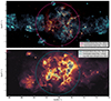 |
Fig. 1. Multi wavelength view of the Cygnus-X star forming region. Upper panel: combination of observations at 500 μm and 8 μm from the Herschel SPIRE and MSX telescopes of the Cygnus X star-forming complex. Radiation at 500 μm (light blue scale) indicates emission from cold dust, while the 8 μm (orange scale) traces photon-dominated regions. Lower panel: continuum observations at 1.42 GHz from the Canadian Galactic Plane Survey (Taylor et al. 2003). A large fraction of this emission is likely thermal free-free radiation by material possibly ionised by Cyg OB2 (Emig et al. 2022). Colour scales are given in arbitrary units. |
Finally, it is worth stressing that close to Cyg OB2 there is a second prominent stellar cluster, NGC 6910, located at a distance of ∼1730 pc and with an estimated age of 5–10 Myr and mass ∼775 M⊙ (Kaur et al. 2020). Astiasarain et al. (2023) have also considered NGC 6910 as a possible contributor to the γ-ray emission in the Cygnus cocoon region; however, as we show in Appendix B we estimate a stellar wind luminosity two orders of magnitude lower than for Cyg OB2. Hence, we decided to exclude NGC 6910 from our analysis.
3. Particle acceleration model
3.1. The wind blown bubble
It is well established that the powerful winds from a YMSC can excavate a cavity inside the ISM. If the cluster is compact enough, namely if the size of the wind termination shock of single stars is larger than the average distance between stars, one can describe the structure and evolution of this cavity as that of a bubble generated by the wind of a single massive star, whose dynamics was investigated by Weaver et al. (1977).
Stellar wind bubbles can be divided in three distinct regions: a central zone, filled with the cold supersonic wind coming from the central source (in our case the cluster core); a cavity composed of hot shocked wind material; an outer shell made of swept-up ISM, piled up in front of the forward shock (FS, propagating in the ISM). The wind region and the cavity are separated by a termination shock (TS) located at a radius Rts, while a contact discontinuity (CD), located at Rcd, separates the cavity from the swept up shell. The forward shock is at Rfs.
The bubble evolution undergoes three different stages that depend on the onset of radiative losses. The typical cooling timescale as a function of the density (n) and temperature (T) of a hot plasma can be written as (Draine 2011):

where n and T are normalised to values typical of the shocked wind and the numerical coefficient refers to Solar metallicity. During the first 1–10 kyr radiative losses are negligible everywhere, hence, the expansion is fully adiabatic (Menchiari 2023). After this initial stage, radiative losses lead to the collapse of the dense outer shell, such that one can assume Rcd ≃ Rfs ≡ Rb, while the hot diluted cavity would continue to expand adiabatically for tens of Myr if conduction were negligible (see below). Eventually, in the late phase, losses begin to impact the evolution of the cavity as well.
Given the age of Cyg OB2 (a few Myrs), the bubble produced by the cluster should be in the intermediate stage of evolution. In such a phase, the bubble size can be obtained by solving the momentum equation of the swept-up shell together with the equation describing the energy variation of the hot gas in the cavity. This leads to the following expression for the bubble radius (see also Morlino et al. 2021):

where ρ0 is the density of the local ambient medium in which the bubble expands, tage is the age of the YMSC and Lw is the wind kinetic luminosity.
As for the position of the TS, this can be calculated from balance between the ram pressure of the cluster wind and the pressure of the hot gas in the cavity, which gives:
where Ṁ and vw are the mass-loss rate and the velocity of the cluster wind, respectively.
Even though radiative losses in the hot cavity are negligible for the first tens of Myr, thermal conduction and turbulent mixing between the hot cavity and the dense swept-up shell can enhance the importance of cooling, resulting in a modification of the system evolution. An approximate way to account for the impact of these processes on the bubble structure is to parameterise the rate of energy losses (Lth) as a fraction ζth of the wind luminosity, such that Lth = ζthLw (El-Badry et al. 2019, Blasi & Morlino 2023). In this way, Eqs. (2) and (3) retain their validity after substituting Lw → (1 − ζth)Lw. This implies that the bubble radius will decrease by a factor (1 − ζth)1/5 while the TS radius will increase by (1 − ζth)−2/5. For example, for ζth = 0.5, Rb (Rts) will decrease (increase) by 13% (30%)1. A further enhancement of the cooling effect may be produced by turbulent mixing. Lancaster et al. (2021) use 3D HD-simulations to show that turbulent mixing can be very effective, producing a bubble evolution closer to the momentum conserving solution than to the energy conserving solution adopted here. Their results suggest a smaller bubble size by a factor ∼2 at few Myr (see also Dwarkadas 2023). However, in that work, cooling is probably overestimated, due to the neglect of magnetic fields, which tend to reduce turbulent mixing and suppress HD instabilities in general (see, e.g. Orlando et al. 2008). Hence, for the purpose of the present work, we consider the adiabatic solution an adequate approximation.
The properties of the collective wind can be estimated using mass and momentum conservation such that the total mass-loss rate and wind speed are:

where Ṁi and vw,i are the mass-loss rate and wind speed of single stars, respectively. The total luminosity will then be  . For the specific case of Cyg OB2, we can use the sample of star selected by Wright et al. (2015). To evaluate Ṁi, we use two different approaches: a theoretical one, as described by Yungelson et al. (2008), and a data-driven one, using empirical relations summarised by Renzo et al. (2017). The detailed calculation is described in Appendix A where we show that the mass-loss rate and luminosity range in an interval Ṁ ∈ [0.7, × 10−4, 1.5 × 10⁻⁴] M⊙ yr−1 and Lw ∈ [1.5 × 1038, 2.9 × 1038] erg s−1. It is worth noticing that this range of values of Lw is compatible with other estimates in the literature based on different approaches. No estimates of Ṁ are available. Unless specified otherwise, in the rest of the paper we use the following reference values for the mass-loss rate and wind luminosity

Assuming that the age of Cyg OB2 is tage = 3 Myr, and that the bubble has expanded in a medium with an average density2 of ρ0 = 20 mp cm−3 (with mp the proton mass), the sizes of the cavity and of the TS are Rb ≃ 86 pc and Rts ≃ 13 pc, respectively. Figure 1 shows the expected size of the bubble compared to the size of the Cygnus-X star-forming complex and the distribution of OB stars observed by Wright et al. (2015). Noticeably, the projected size of Rb is compatible with the extension of the bubble-like structure observed in 21 cm continuum. Notice also that the estimated ranges of Ṁ and Lw lead to an uncertainty on Rb and Rts of ∼20%.
Finally we notice that the bubble evolution may be affected by possible SN explosions that could have occurred in the recent past. However, no clear signatures of SNRs have been detected in the Cygnus OB2 association, and, if the actual age of Cyg OB2 is ∼3 Myr, as assumed here, the estimated energy injected by SNe should be anyway negligible with respect to the wind input (see Appendix B).
3.2. Cosmic-ray distribution
Let us now consider the scenario in which CRs are accelerated at the TS of the collective wind. An analytical solution to this problem has been presented by Morlino et al. (2021) while a fully numerical approach has been developed by Blasi & Morlino (2023)3. Hence, the reader is referred to those papers for further details. Here, we use the former approach. However, in that work, the distribution function at the TS was found recursively. This would be computationally too expensive to implement in the current work, which aims at an exploration of the parameter space. Therefore, in order to speed up the calculation when performing a fit to the γ-ray data, we adopt an analytical fit to the full solution.
The system can be briefly described as follows: particles are accelerated at the TS via the diffusive shock acceleration process, and subsequently escape from the acceleration site experiencing advection and diffusion in the hot bubble until they reach the forward shock. From there, CRs are free to leave the system by diffusing in the unperturbed ISM. Given the slow expansion rate of the cavity, the system can be assumed to be stationary, and if one assumes a radial symmetry, the distribution f(r, E) of CRs can be found by solving the following steady-state transport equation in 1D spherical symmetry:
![$$ \begin{aligned} \frac{\partial }{\partial r} \left[ r^2 D(r,p) \frac{\partial f}{\partial r} \right] - r^2 u(r) \frac{\partial f}{\partial r} + \frac{\mathrm{d} [r^2 u(r)]}{\mathrm{d}r} \frac{p}{3} \frac{\partial f}{\partial p} +r^2 Q(r,p) = 0 ,\end{aligned} $$](/articles/aa/full_html/2024/06/aa48817-23/aa48817-23-eq9.gif)
where p is the particle momentum, u(r) is the plasma speed, and D(r, p) is the diffusion coefficient. The source term Q(r, p) describes particle injection taking place at the TS:
where nw is the density immediately upstream of the TS, vw is the speed of the cold wind, and ηinj is the fraction of particle flux that undergoes the acceleration process.
The solution to Eq. (8) can be found as follows. First, the equation is solved separately in the wind region (upstream the TS), in the cavity (downstream the TS) and in the unperturbed ISM. Then, the three solutions are joined using particle flux conservation at r = Rts and r = Rb. Finally, one needs to specify two boundary conditions: one at the center of the bubble, where the flux is assumed to be null, and the other at infinity where f matches the distribution of the galactic CR sea, fgal. The expression for fgal is taken from the Galactic CR proton spectrum as measured by AMS-02 data (Aguilar et al. 2015). The CR radial distribution in the wind region (fw), in the cavity (fb) and outside the bubble (fout) is found to be respectively:
![$$ \begin{aligned} f_{\rm w}(r,p)\simeq f_{\rm ts}(p) \cdot \exp \left[ -\int _r^{R_{\rm ts}} \frac{{ v}_{\rm w}}{D_{\rm w}(r^\prime ,p)} \mathrm{d}r^\prime \right] ,\end{aligned} $$](/articles/aa/full_html/2024/06/aa48817-23/aa48817-23-eq11.gif)
![$$ \begin{aligned} f_{\rm b}(r,p)= \frac{f_{\rm ts}(p) \left[e^{\alpha } + \beta (e^{\alpha _{\rm b}} - e^{\alpha }) \right] + f_{\rm gal}(p) \,\beta (e^\alpha -1)}{1+\beta (e^{\alpha _{\rm b}}-1)} ,\end{aligned} $$](/articles/aa/full_html/2024/06/aa48817-23/aa48817-23-eq12.gif)

where

The terms Dw, Db, and Dout are the diffusion coefficients in the wind region, in the cavity and outside the bubble, respectively, while vb = vw/4 is the plasma speed immediately downstream of the TS (assumed to be strong). Notice that Eq. (10a) is a first-order approximation to the full solution presented by Morlino et al. (2021), but it is fully adequate for the aim of this work. fts is the distribution at the TS, which can be expressed as:
where c is the speed of light, ϵcr is defined as the fraction of wind luminosity converted into CR luminosity, namely Lcr = ϵcrLw, while the function Λp is the usual normalization factor:
with x = p/(mpc). The function Γ(p) contains information about the spherical geometry and the diffusion coefficients in both the wind region and the hot cavity. Γ(p) has a complicated expression defined recursively (Morlino et al. 2021), but a good approximation is:
![$$ \begin{aligned} e^{\Gamma (p)} \simeq \left[ 1 + a_1 \left(\frac{p}{p_{\max }} \right)^{a_2} \right] e^{- a_3 (p/p_{\max })^{a_4}} \ , \end{aligned} $$](/articles/aa/full_html/2024/06/aa48817-23/aa48817-23-eq19.gif)
where pmax is the ‘upstream’ maximum momentum defined by the condition that the upstream diffusion length is equal to the shock radius, i.e. Dw(pmax) = vwRts4. a1…a4 are parameters that mainly depend on the adopted diffusion model and are obtained by fitting Eq. (14) to the full solution. The values of these coefficients are reported in Table 1 for the three different diffusion models used in this work.
A final remark before the end of this section concerns proton energy losses. Equation (8) does not account for energy losses due to inelastic interactions which, in general, are important if the average density in the bubble is ≳10 cm−3 (Blasi & Morlino 2023). In particular, the shape of proton spectrum can be significantly affected only for nb ≳ 20 cm−3 while heavier nuclei can suffer substantial losses even at lower density, given that the inelastic cross section increases with the atomic number A as ∝A0.7. Considering only the mass injected by the stellar winds, the bubble density would be extremely low (e.g. nb ∼ 5 × 10⁻³ cm−3 for Ṁ = 10−4 M⊙ yr−1 and Rb = 86 pc), but it can substantially increase due to the evaporation of the shell (Castor et al. 1975). The mass evaporation rate from the cold shell, given in terms of the cluster properties (Menchiari 2023) is:

Using again the parameters of Cyg OB2 the bubble density can rise up to ∼0.1 cm−3, still too small to be relevant for inelastic collisions. A larger density can be obtained if the shell fragments in compact dense clumps (dense enough that the wind is not able to blow them away) or if there were pre-existing molecular clouds in the bubble region. Whether or not clumps affect the final CR spectrum depends on a combination of their filling factor and the value of the diffusion coefficient inside the clumps. In Sect. 4, we show that the column density measured in the Cygnus region thorough 12CO and HI lines suggests an average density ≲8.5 cm−3, supporting the presence of clumpy structure in the region. With such a value, energy losses of protons remain small enough that the resulting γ-ray spectrum should not be significantly affected (Blasi & Morlino 2023).
3.3. Diffusion coefficient in the wind bubble
The particle distribution function strongly depends on the diffusion coefficient determined by the magnetic turbulence inside the bubble, which remains the most uncertain parameter of the problem. As discussed in Blasi & Morlino (2023) the CR-self generated turbulence is not strong enough to allow efficient particle confinement. Most probably the turbulence is generated by the wind itself through MHD instabilities due to inhomogeneity and non-stationarity of the wind flow. Hence, we assume that in the upstream some fraction ηB of the wind luminosity is converted into magnetic flux
At the TS we assume that the magnetic field is compressed by the shock, so that, for a strong shock and an isotropic turbulent field, we have  . The type of diffusion associated with turbulence depends on the details of the cascade. We consider here both Kolmogorov (Kol) and Kraichnan-type (Kra) of cascade such that the diffusion coefficients are

where vp is the particle velocity, rL = cp/(eδBinj) is the particle Larmor radius, Linj the turbulence injection scale, and δBinj = δB(Linj). For particles having rL > Linj we assume D ∝ p2 as predicted by quasi-linear theory and confirmed by numerical simulations (see e.g. Subedi et al. 2017). We do expect Linj to be comparable to the size of the cluster core (Linj ∈ [1, 2] pc). However, more spatial scales may be connected to the generation of turbulence, from the TS size, down to the typical distance between stars. If the power injected at all those scales is of the same order, one would rather expect a flatter turbulence, similar to Bohm’s. For this reason we explore here also Bohm-like diffusion, described as
The impact of these three different types of diffusion on the spatial profile of CRs is shown in Fig. 2, where we assume fgal = 0. The profiles are calculated using a wind luminosity Lw, ref, and a particle spectral index at injection s = 4. One can readily see that Kolmogorov turbulence results in a decreasing profile for r > Rts, while for Bohm diffusion the profile is flat at all relevant energies for Rts < r < Rb. The Kraichnan case is intermediate, resulting in a distribution that is flat below ∼10 GeV and peaked above such energy. The departure from a flat distribution occurs when diffusion dominates over advection. The transition energy at which this happens can be estimated comparing the timescales of the two processes: the advection timescale
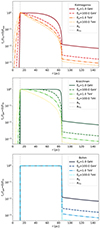 |
Fig. 2. Radial CR distribution normalised to its value at the termination shock in the case of Kolmogorov (top panel), Kraichnan (central panel), and Bohm (bottom panel) turbulence. In these plots, the contribution of the Galactic CR sea to fcr has not been included. |
and the diffusion timescale,

Using the reference values for Cyg OB2 discussed in Sect. 3.1, we find that tadv ≃ τd at energies of ∼20 GeV, ∼2 TeV, and ∼300 TeV for Kolmogorov, Kraichnan, and Bohm cases, respectively.
In addition to the spatial profile, the diffusion coefficient also determines the maximum achievable energy. As discussed by Morlino et al. (2021) the maximum energy results from the combination of three elements: the confinement time upstream and downstream of the shock, plus effective jump conditions at the shock due to the spherical geometry. The latter condition determines the sharpness of the cutoff. It is useful to report here the maximum energy given by the upstream condition, i.e. Dw(Emax)/vw = Rts, because it is the one that appears in Eq. (14). Considering Eqs. (3), (5), and the expression for the diffusion coefficients, the maximum energies for the three cases are:

In Sect. 5, we separately consider the three different types of diffusion, comparing the resulting γ-ray emission with observations of the Cygnus cocoon.
4. Hadronic γ-ray emission
Accelerated protons give rise to γ-ray emission through the decay of neutral pions produced in inelastic collisions. The resulting spectrum and morphology will depend on the distributions of both CRs and target medium. The differential γ-ray flux coming from a given volume V of the sky is given by
where d is the distance of the considered volume, Ep and Eγ are the CR kinetic energy and the γ-ray energy respectively, while σ is the cross-section for γ-ray production (which we take from Kafexhiu et al. 2014). The CR distribution, fcr(Ep, r), is the one described in Sect. 3.2, while n(r) represents the gas density in and around the star cluster. As discussed above, the presence of clumps of neutral material is likely to dominate the mass of the target, especially if located within the bubble, and therefore, below, we determine the amount of gas from observations rather than relying on the theoretical profile of the bubble density distribution.
Estimating the amount of gas in the Cygnus region based on observations is not straightforward because this region is located at a galactic longitude where the differential galactic rotation results in low radial velocities, with values compatible with the typical gas dispersion motion, which prevents a reliable modelling of the ISM profile along the line of sight (Schneider et al. 2006). For the sake of simplicity, we assume here that the gas is uniformly distributed along the line of sight in a range Δz = ±400 pc around Cyg OB2 position, hence, without considering the density profile of the bubble (in Sect. 6 we further discuss the uncertainty due to such an assumption). Our choice of Δz follows from the total extent of 800 pc for the distribution of dust towards the Cygnus-X star forming complex (Green et al. 2019). We further assume that the target medium only contains molecular and neutral gas, and therefore neglect the contribution of ionised gas. To quantify the amount of neutral hydrogen, we use 21 cm line data from the Canadian Galactic Plane Survey (CGPS; Taylor et al. 2003). For the molecular component, we use high-resolution observations of 12CO J(1–0) spectral line from the Nobeyama radio telescope (Takekoshi et al. 2019) in combination with the data from the composite galactic survey of Dame et al. (2001). Although the kinetic ambiguity prevents an accurate location of the gas along the line of sight, we apply to all observations a velocity cut between −20 km s−1 and 20 km s−1, so as to remove the contribution from gas located in the Perseus and Outer arms. We calculate the neutral hydrogen column density using the standard approach described by Wilson et al. (2009):
![$$ \begin{aligned} \left[ \frac{N_{\rm HI}}{\mathrm{cm}^2} \right] = - 1.8224 \times 10^{18} \left[ \frac{T_{\rm s}}{K} \right] \int _{-20}^{20} \log \left( 1 - \frac{T^\mathrm{HI}_{\rm br} ({ v})}{T_{\rm s}-T_{\rm bg}} \right) \left[ \frac{\mathrm{d}{ v}}{\mathrm{km\,s}^{-1}} \right], \end{aligned} $$](/articles/aa/full_html/2024/06/aa48817-23/aa48817-23-eq32.gif)
where  is the observed line brightness temperature, Ts is the spin temperature assumed to be 150 K, and Tbg = 2.66 K is the brightness temperature of the cosmic microwave background at 21 cm. For the molecular hydrogen, we estimate the column density using the standard XCO conversion factor:
![$$ \begin{aligned} N_{\rm H_2} = X_{\rm CO} \int _{-20}^{20} T_{\rm br}^\mathrm{CO}({ v}) \left[ \frac{\mathrm{d}{ v}}{\mathrm{km\,s}^{-1}} \right], \end{aligned} $$](/articles/aa/full_html/2024/06/aa48817-23/aa48817-23-eq34.gif)
with XCO = 1.68 × 10²⁰ mol. cm−2 km−1 s K−1 as found by Ackermann et al. (2011). The total gas column density is Ntot = (NHI + 2NH2) with an average density of n(r) = Ntot/Δz. The resulting column density is shown in Fig. 3, together with the mean gas density averaged over the angle. These are compatible with other estimates (Ackermann et al. 2011; Aharonian et al. 2019). The average gas density in the entire region is ngas = 8.5 if one considers the gas uniformly distributed in the whole cylinder of 800 pc size. However, the density in the bubble could be smaller if the majority of the gas is located outside of it.
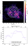 |
Fig. 3. Gas column and number density in the vicinity of Cyg OB2. Top panel: total target column density considering the ISM in the neutral and molecular phases. The column density of HI has been evaluated using the 21 cm line observation from the CGPS, while for the molecular gas, we used a combination of 12CO observations from the Nobeyama radio telescope and the data from the 12CO galactic plane survey by Dame et al. (2001). All the observations are kinematically cut selecting only the gas between −20 and 20 km s−1. White rings represent the regions used by Aharonian et al. (2019) and Abeysekara et al. (2021) to probe the γ-ray radial profile. The radii of the different circles correspond to angular sizes of 0.61°, 1.19°, 1.8° and 2.21°. Bottom panel: average gas density profile in the Cygnus region for each annulus. |
Because γ-ray data available in the literature are provided for annuli around the center of Cyg OB2, it is useful to express the γ-ray flux as a function of the radial coordinate projected along on the sky, l. Considering that  , where z is the distance from the center of the cluster projected along the line of sight, the γ-ray flux from an annulus of thickness Δl is
where  is the average ISM density profile along the line of sight calculated from the column density maps and ξ(l′,Eγ) is defined as
By varying the integration boundaries in z, Eq. (28) can also be used to estimate the total γ-ray flux from the Cocoon.
5. Comparison with observations
By comparing the spectrum and morphology of the γ-ray emission with the predictions of our model, we can find best fit values of Lw, s, and ϵcr5. Subsequently, we can evaluate the overall validity of our proposed model by looking at the consistency between the best-fit value of Lw and that inferred from the stellar population as calculated in Sect. 2. In order to simplify the analysis, we fix all the other source parameters to the values discuss in Sect. 2tage = 3 Myr, Ṁ = Ṁref yr−1, ρ0 = 20 mp cm−3, ηB = 0.1, Linj = 2 pc and distance d = 1.4 kpc. GeV data of the Cygnus Cocoon are from Fermi-LAT 4FGL (4FGL J2028.6+4110e) (Abdollahi et al. 2020), TeV data are from Argo (ARGO J2031+4157) (Bartoli et al. 2014) and HAWC (HAWC J2030+409) (Abeysekara et al. 2021). The Cygnus region was also detected by LHAASO (J1908+0621) in 2021 (Cao et al. 2021) but the detailed spectrum has not yet been published6.
We highlight the fact that we do not include the γ-ray emission produced by the foreground CR sea (i.e. we assume fgal = 0 in Eq. (10)), as the diffuse component has been already subtracted from the data that we use. The best-fit parameters are found by χ2 minimisation of the spectral properties over a region of 2.2° radius centred on the stellar cluster (corresponding to a projected radius of ∼54 pc). Given that the spectrum of extended sources is usually fitted with a 2D symmetric Gaussian, with wings extending beyond the region of interest, the flux must be properly rescaled7.
Once we obtain the CR distribution that best describes the observed spectrum, we compare the corresponding γ-ray radial profile with the ones obtained from Fermi-LAT (Aharonian et al. 2019) and HAWC data (Abeysekara et al. 2021). To this purpose, we calculate the total γ-ray luminosity in four rings centered on Cyg OB2, with projected sizes of 0–15 pc, 15–29 pc, 29–44 pc, and 44–54 pc (see Fig. 3). The corresponding surface brightness in the energy range [E−, E+] is:

where Ωring is the annulus area and the energy ranges are [10, 300] GeV for the Fermi-LAT and [1, 250] TeV for HAWC.
5.1. Kolmogorov case
Assuming Kolmogorov-like diffusion, we find that the minimum χ2 corresponds to Lw = 5 × 1039 erg s−1, which is the upper boundary of our interval. The χ2 behaviour makes it clear that even larger values would be preferred. While not corresponding to a global minimum, Lw = 5 × 1039 erg s−1 provides a good fit to the data (see top panel of Fig. 4), with reasonable values of the other parameters (see Table 2). However, such a luminosity is more than a factor 10 higher than the value estimated in Sect. 2, which makes Kolmogorov-like diffusion incompatible with our model: Kolmogorov turbulence does not provide efficient confinement of the particles resulting into a low maximum energy and a very broad cutoff. As a result, a cutoff that in γ-rays shows at ∼100 TeV corresponds to a proton maximum energy of ≃ 20 PeV (see Table 2).
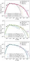 |
Fig. 4. Spectral energy distribution of the expected hadronic γ-ray emission extracted from a region of 2.2° centred on Cyg OB2. Lines in different panels refer to Kolmogorov (top panel), Kraichnan (middle panel), and Bohm cases (bottom panel). Solid lines always represent the best-fit curves, whose underlying parameters are summarised in Table 2. Other line-types correspond to the values of the parameters listed in the legend inside each panel. |
Best-fit parameters values and main system properties for three different models.
Indeed by fixing Lw to the best value inferred from the stellar population, i.e. Lw, ref, the corresponding γ-ray spectrum dramatically fails in reproducing the data (Fig. 4). We also verified that no good agreement can be achieved by increasing the level of magnetic turbulence while keeping Lw = Lw, ref: assuming the unrealistically high value of ηB = 0.9, the calculated flux remains well below the observations for Eγ ≳ 1 TeV (Fig. 4).
5.2. Kraichnan case
For Kraichnan-like diffusion the global χ2 minimum corresponds to Lw = 1.28 × 1039 erg s−1 (case labelled as Kraichnana in Table 2, shown by the solid line in the middle panel of Fig. 4), which is still a factor of ∼6 higher than Lw, ref and a factor of 4 larger than the maximum derived in Appendix A. Again, such a high wind luminosity is required in order to fit the very high energy part of the spectrum. A wind luminosity of 1.28 × 1039 erg s−1 corresponds to Emax = 3.97 PeV in Eq. (23). In principle, the spectrum can still be reproduced with a lower wind power by modifying the other cluster parameters appropriately: using Eq. (23), and setting Lw = 3× 1038 erg s−1, Ṁ = 0.7 × 10⁻⁴ M⊙ yr−1, ηB = 0.35, Linj = 0.7 pc, we find a similar value of Emax. With this choice of parameters, the best fit values for the spectral index and the efficiency of CR production are s ≃ 4.23 and ϵcr ≃ 0.018, respectively (case labelled as Kraichnanb in Table 2, shown by the dotted line in the middle panel of Fig. 4). Notice that the parameter values are rather extreme but still within the limits inferred from the stellar population study.
Concerning the morphological study of the emission, since the CR distribution is very similar in both cases, we illustrate the spatial properties of the γ-ray emission only for case Kraichnanb.
The top panel of Fig. 5 shows the comparison of our results with the radial profile derived from Fermi-LAT and HAWC data. Concerning the former, one can clearly see that our predicted flux is not in agreement with that estimated by Aharonian et al. (2019). First of all, we should note that the spectrum by Aharonian et al. (2019) is a factor ∼2 lower than the one published in the 4FGL (used in this analysis; see middle panel of Fig. 4). In addition, even when this factor of 2 is taken into account, the resulting radial profile (grey points in top panel of Fig. 5) decreases too fast from the inner to the outer region. This trend is especially surprising in light of HAWC data, showing a flat radial profile. As we discuss in more detail in Sect. 6, any advection-diffusion model would predict a flatter profile at lower energies.
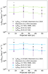 |
Fig. 5. Comparison with observations of the expected γ-ray surface brightness radial profile for the Kraichnan (upper panel) and Bohm (bottom panel) cases. Black squares correspond to the measurements by Fermi-LAT (Aharonian et al. 2019), while purple circles indicate the surface brightness observed by HAWC (Abeysekara et al. 2021). Grey squares represent Fermi-LAT measurements rescaled by a factor of 2. Diamonds and crosses indicate the surface brightness values based on our model, at energies of 10 < Eγ < 316 GeV and 1 < Eγ < 251 TeV respectively. |
5.3. Bohm case
Finally, for the Bohm case we found the global χ2 minimum for Lw = 1.9 × 1037 erg s−1, with corresponding best fit values of s ≃ 4.27 and ϵcr ≃ 0.13 (case Bohma in Table 2 and solid line in bottom panel of Fig. 4). In contrast with the previous cases, the required wind luminosity is lower by almost one order of magnitude with respect to the lower bound of the range of values estimated in Sect. 2. In fact, Bohm-like turbulence is the most effective at confining particles and has the strongest energy dependence, resulting in the highest maximum energy (for fixed Lw) and sharpest cut-off. Furthermore, the low diffusion coefficient within the bubble prevents the escape of high-energy particles from the system, which negates the suppression of emission at very high energies. This can be seen by noticing that the spectrum obtained for Lw = Lw, ref overshoots the observations in the cutoff region (dashed line in the Fig. 4).
We then tried to fit the spectrum fixing Lw = Lw, ref, while allowing ηB to vary. We found the global χ2 minimum for ηB = 2.4 × 10⁻³, with an associated spectral index and CR efficiency of s ≃ 4.27 and ϵcr ≃ 0.022 (case Bohmb in Table 2 and dotted line in Fig. 4). The corresponding maximum energy is Emax ≃ 470 TeV, only slightly lower than the value found for the case Bohma.
5.4. Parameter degeneracy
The solutions presented in the previous sections are not unique because there is a degeneracy in the parameter space: for each assumed diffusion coefficient, a class of solutions with a similar χ2 value can be identified. These solutions are characterised by relations between the parameters that can be approximated by the analytical expressions we provide below.
Once the diffusion coefficient has been chosen, the shape of the γ-ray emission is mainly determined by three quantities: the spectral index of the injected particle distribution, s, the flux at low energies, ϕ0, and the value of the maximum energy, Emax. We need to look for the dependencies of these observables on the unknown parameters, Lw, ϵcr and ηB.
The spectral slope has a very mild dependence on those parameters: it is mainly determined by the diffusion coefficient. Hence, if we fix the latter, s is uniquely determined. The flux normalization, instead, is roughly proportional to ∼ftsngasRb. The linear dependence on Rb results from assuming that the bubble radius is larger than the size of the observed region (as is the case for all solutions discussed above) hence the emission is integrated over a cylinder. Now, considering the dependencies of fts (Eq. (12)) and Rb (Eq. (2)), we obtain  , where we have assumed that the wind speed remains roughly constant by changing the wind luminosity, which is a good approximation for YMSCs. The maximum energy scales instead as
  where
where  ,
,  or
or  for Kolmogorov, Kraichnan or Bohm diffusion, respectively. Therefore, once an optimal solution has been identified, having parameters {Lw, 0, ϵcr, 0, ηB, 0}, then, by varying the wind luminosity in the range of allowed values, all solutions having

will provide an acceptable fit to the γ-ray spectrum. On the other hand, if the wind luminosity is known, then, for each diffusion coefficient, there is only one single solution.
6. Discussion
6.1. Spectral energy distribution
Table 2 summarises our results. The first thing to notice is that all cases require a particle injection slope s > 4. This is softer than the standard spectral index expected from diffusive shock acceleration at strong shocks, such as the ones found in compact and powerful star clusters. This result is not too surprising: also young SNRs, hosting very strong shocks, typically show spectra steeper than p−4, a feature that can result from several different mechanisms. In the case of SNRs a possible explanation is connected with the magnetic waves that scatter off particles: if the wave speed is mainly directed away from the shock (either upstream or downstream): the effective compression factor felt by particles is reduced, resulting into a steeper spectrum. Such an effect has been found for shocks where the magnetic turbulence is self-generated by CRs (Haggerty & Caprioli 2020; Cristofari et al. 2022) however it is not clear whether the same result applies for magnetic turbulence generated by MHD instabilities, as seems the case for YMSCs. Another possibility is that the shock is affected by a non perfect central symmetry of the SC. In the specific case of the Cyg OB2 association, 50% of the brightest stars are enclosed in a volume of radius ∼5 pc. Hence, the presence of stars outside this volume and closer to the position of the TS can affect the structure of the shock itself. Finally, strong cooling of the wind bubble can also reduce the velocity jump if the bubble temperature drops below ∼106 K.
We also note that the best-fit spectral index is substantially steeper than the value of 4.08 inferred in Blasi & Morlino (2023). The reason is due to the different cross section used for pp scattering. While Blasi & Morlino (2023) used the parametrisation by Kelner et al. (2006), here we adopted the one derived by Kafexhiu et al. (2014) which is more accurate at low energies (the most relevant in determining the spectral slope). An additional difference is that here we have neglected the effect of energy losses due to inelastic proton-proton collisions, which, on the contrary, have been extensively studied by Blasi & Morlino (2023). However, as shown in Sect. 4, the upper limit to the total average gas density in the bubble is ∼8.5 cm−3, a small enough value so that the energy losses only marginally affect the spectrum of protons.
Another important result is the low value inferred for the CR acceleration efficiency, which is of the order of 1% (with the exception of the case Bohma for which we found ϵcr = 13%), or a factor of 3–10 smaller than what is usually estimated for SNR shocks. However, remembering that the γ-ray flux is proportional to ϵcr × ngas, the acceleration efficiency is likely underestimated by our calculation if, as discussed in Sect. 4, the target gas is mainly distributed outside the wind bubble. On the contrary, the additional uncertainties on ϵcr due to Cyg OB2 distance (e.g. if the cluster is indeed at 1760 pc, as proposed by Berlanas et al. 2019), is negligible in terms of physical interpretation.
A significant difference between the Kraichnan and Bohm models is the nominal value of the maximum energy reached by the particles (≃4 PeV for Kraichnan and ≃0.5 PeV for Bohm). Despite such a difference, the γ-ray spectra of the two cases are remarkably similar, with an exponential cutoff feature in the γ-ray spectrum that in both cases is located at a few tens of TeV. This, once more, is due to a shallower shape of the cutoff in the Kraichnan case compared to the Bohm one (Morlino et al. 2021). This fact highlights the very important role played by the modelling of particle transport when deriving the maximum energy achieved by the accelerator from the spectrum of its γ-ray emission.
Finally, we notice that all cases presented here underestimate the γ-ray flux at energies ≲100 MeV with respect to the values reported in the Fermi-LAT 4FGL catalogue. The most plausible explanation for such a discrepancy is that the background adopted in the Fermi analysis is underestimated. Indeed, the analysis used for the 4FGL is generic and is not specific to the case of the Cygnus region. In fact, other analyses, such as those presented by Aharonian et al. (2019) and Astiasarain et al. (2023), have not included data below a few hundred MeV, precisely because the background subtraction is highly uncertain. Another possible explanation is that an additional contribution, possibly coming from the inverse Compton scattering of electrons or bremsstrahlung, may be present. As discussed in Sect. 6.3, while dominant leptonic emission at the highest energies is highly disfavoured, currently a substantial leptonic contribution at the lowest γ-ray energies cannot be ruled out.
6.2. Spatial profile
As shown in Sect. 5, Bohm and Kraichnan cases predict a flat morphology in the γ-ray emission profile, in both the Fermi-LAT and HAWC energy bands. The uniformity of the profile is a result of the advection dominated transport of CRs, which makes the distribution constant in space. While this result is expected in the case of Bohm-like turbulence (see Fig. 2), for the Kraichnan case in the HAWC energy band it might seem at odds with naive expectations, because for E ≳ 10 TeV the diffusion time becomes shorter than the advection one, producing a decrease of the CR density. The reason why we do not see such a decrease in the γ-ray profile is that we are probing the morphology in a projected sky area of about 54 pc, smaller than the size of the bubble, which for our best-fit Kraichnan case is Rb ≃ 93 pc. As described in Sect. 3.2, since the advection velocity scales as ∝r−2, areas close to the TS will be characterised by high advection velocities, resulting in advection dominated transport. This can be easily understood by looking at Fig. 6, which shows the timescales of advection and diffusion in a region of size 54 pc. For the Kraichnan (Bohm) case, advection dominates up to energies of ∼10 TeV (100 TeV). We note that if the distance of Cyg OB2 were 1760 pc, the region tested would be of 67 pc, still smaller than the size of the bubble, hence, we would not expect a significant change in the radial morphology.
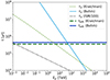 |
Fig. 6. Comparison between diffusion (thin lines) and advection (thick lines) timescales for the Kraichnan (green dashed lines) and Bohm (blue solid lines) cases. The black dotted line shows the diffusion time in the case of a diffusion coefficient with the same slope as that in the standard interstellar medium normalised a factor of 100. All timescales are calculated considering only the region used for the morphological analysis, i.e. substituting Rb with 54 pc in Eqs. (20) and (21). |
Indeed, our constant CR distribution, after convolution with the gas distribution, is consistent with HAWC observations, while it disagrees with the radial morphology inferred from Fermi-LAT data (Aharonian et al. 2019). The centrally peaked profile shown by the latter cannot be reconciled with the HAWC morphology within our model: if advecion is dominant in the HAWC band, it must dominate also in the Fermi-LAT band, independently of the model parameters.
In fact, based on Fermi-LAT data, Aharonian et al. (2019) deduced a CR distribution decreasing with radius as 1/r, as one would expect in the case of continuous injection of CRs from a central source and diffusion dominated transport. These authors used the γ-ray luminosity at Eγ ≥ 1 TeV to infer the diffusion coefficient at ∼10 TeV, obtaining a value ∼100 times smaller than the average value in the ISM. If we extrapolate this finding down to 100 GeV (the proton energy corresponding to the γ-ray emission at Eγ ≈ 10 GeV), assuming the Kolmogorov scaling ∝E1/3, we obtain D(100 GeV)∼1027 cm2 s−1. Recalling that diffusion dominates if τdiff ≪ τadv, we can put an upper limit on the average advection speed that reads vadv ≪ D(p)/L. Quantitatively:
![$$ \begin{aligned} { v}_{\rm adv} \ll 60 \left[\frac{D(100\,\mathrm{GeV})}{10^{27}\, \mathrm {cm}^2 \mathrm {s}^{-1}}\right] \left( \frac{\theta }{2.2^{\circ }}\right)^{-1} \left( \frac{d}{1.4\, \mathrm{kpc}}\right)^{-1}\, \mathrm{km\,s}^{-1}\,, \end{aligned} $$](/articles/aa/full_html/2024/06/aa48817-23/aa48817-23-eq47.gif)
where θ is the angular distance from Cyg OB2. Such a value is much smaller than the average flow speed in the bubble in standard models of bubbles around YMSCs, implying that a pure diffusion regime is in tension with the existence of a bubble.
On the other hand, the model we propose naturally explains the HAWC morphology, which is not easy to reconcile with a pure diffusive profile. If a wind bubble exists, indeed, additional processes not included in our model must be responsible for the Fermi-LAT morphology. A possibility is that, in the Fermi-LAT band, the contribution of leptonic Inverse Compton emission might be relevant: leptons accelerated at the TS would suffer energy losses while advected outward and a centrally peaked profile is naturally expected. Another possible scenario that can accommodate both HAWC and Fermi-LAT data is one in which, upstream of the TS, particle acceleration up to tens of GeV is contributed by single star winds. If there is sufficient target for γ-ray emission before the TS, these CRs would provide an additional, centrally peaked low energy contribution. A quantitative assessment of these scenarios is left for future work.
6.3. Possible leptonic contribution
Above, we neglect a possible leptonic contribution to the γ-ray emission. The main reason for this is that recent studies, based on different pieces of observational evidence, tend to disfavour the dominance of leptonic emission beyond 1 TeV. First of all, Guevel et al. (2023) considered the lack of non-thermal X-ray emission: upper limits on the X-ray flux suggest that the IC scattering does not contribute more than approximately one-quarter of the observed γ-ray emission at 1 TeV, assuming an equipartition magnetic field of ∼20 μG. In addition, analysing the last 10 yr of IceCube data, Neronov et al. (2023) find a 3σ excess of neutrino events from an extended Cygnus Cocoon, at a flux level compatible with the assumption that the observed γ-ray emission above ∼1 TeV is due to hadronic interactions.
Moreover, there is also a theoretical motivation that strongly disfavours the possibility that leptonic emission dominates the γ-ray spectrum at the highest energies if acceleration is limited to the TS, as we assume in this work: the maximum energy that electrons can achieve at the wind TS is too low due to energy losses. This can be easily shown equating the acceleration time,  with the energy loss time,
  where the IC losses account for the CMB (UCMB) and star light (U*) photon fields at the location of the termination shock, RTS. For starlight, we use
  , where ℒ is the total luminosity of the star cluster estimated by integrating the stellar luminosity from Eq. (B.4) over the stellar IMF: this leads to U⋆ ≃ 30 eV cm−3. We estimate tIC using the full Klein-Nishina cross section in the approximate expression obtained by Khangulyan et al. (2014). In order to obtain a conservative upper limit to the electron maximum energy, we minimise the ratio between the timescales for acceleration and losse. By using the Bohm diffusion coefficient and the upper limit for the wind speed, which is ∼2800 km s−1, we find that Ee, max ≃ 180 TeV is found for a magnetic field of ∼1.6 μG. If, instead, we chose the Kraichnan diffusion with Lc = 2 pc as adopted in Sect. 3.3, we get Ee, max ≃ 40 TeV for a magnetic field of 1.9 μG. We notice that these values of the magnetic field are one order of magnitude below equipartition. Values closer to equipartition, B ∼ 20 μG, would limit the electron energy to < 70 TeV even in the most favourable scenario of Bohm diffusion. Hence, in the most optimistic scenario of Bohm diffusion, IC emission can reach ∼100 TeV, but with a sharp cutoff due to the Klein-Nishina suppression. Hence, it would be very difficult to account for the LHAASO data up to ∼1 PeV.
Moving to lower energies, we first notice that the spectral shape below ∼1 GeV in the Fermi-LAT data suggests the presence of the pion bump, a spectral signature difficult to explain with leptonic emission only, without invoking some fine-tuning either in the particle spectrum (suitably broken power-law) or in the combination of the contributing radiation backgrounds. In addition, if the IC scattering is not negligible at the highest energies, the typical shape of IC emission would imply that the same process only marginally contributes at energies below ∼10 GeV (Abeysekara et al. 2021). An additional contribution at lower energies could come from the non-thermal bremsstrahlung. We can estimate which would be the electron acceleration efficiency, ηel, needed to have a significant bremsstrahlung emission in the GeV energy band. The luminosity due to bremsstrahlung for photons above energy E0 can be written as

where τloss is the timescale for electron energy losses, τbrem is the timescale for bremsstrahlung radiation, and  is the fraction of wind luminosity converted into electrons with energy > E0 and is connected to the full efficiency through
  . Using τbrem = 5 × 10⁶(n/8 cm−3)−1 yr (Aharonian 2004), s = 4.3, and assuming that bremsstrahlung is responsible for the whole γ-ray emission in the Fermi-LAT band, L1−100 GeV = 9 × 1034 erg s−1 (Ackermann et al. 2011), we estimate ηel ≃ 3% for the reference value of the wind luminosity of 2 × 1038 erg s−1. This efficiency is about two orders of magnitude larger than what usually estimated for SNR shocks. Hence, it seems rather unlikely that bremsstrahlung can dominate the γ-ray emission, although it cannot be completely ruled out. In any case, a detailed analysis of leptonic emission is ongoing and will be presented in a forthcoming article.
6.4. Possible future tests
Considering the results obtained so far, our model can account for the γ-ray emission from Cygnus OB2 both with the Kraichnan’s and Bohm’s turbulence description and associated transport, albeit with the caveats mentioned in the previous sections. From the point of view of the spectral analysis, the difference in the χ2 value is not statistically significant to make a case preferred with respect to the other. In terms of radial morphology, both models lead to a flat profile.
In principle, other pieces of information can be used to break the degeneracy between the cases. First, good knowledge of the structure and size of the bubble generated by the cluster would provide additional constraints on the wind power and mass-loss rate, potentially breaking the degeneracy between the two cases. This kind of information could be provided by a deep study of the thermal diffuse X-ray emission produced by the hot plasma in the bubble: X-ray data from eRosita would be ideal for such an analysis.
Once the bubble is properly identified, one could analyse the γ-ray emission in regions close to its border. Figure 7 shows the γ-ray spectrum extracted at different projected distances from the center of the bubble. The spectral shape from a region close to the bubble border could be used to discriminate between different diffusion coefficients. In this regard, data gathered by wide-field telescopes like CTA and LHAASO would play a pivotal role.
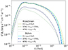 |
Fig. 7. Expected hadronic γ-ray spectra extracted from rings at projected distances of |


Another possible way to discriminate between the two cases is to consider the γ-ray emission originating from dense molecular clouds that are possibly found inside the bubble. As mentioned in Sect. 2, Cyg OB2 is surrounded by a significant number of molecular clouds, some of which are observed to be in direct interaction with the stellar winds and radiation of the cluster. Among the clouds close to Cyg OB2, DR21, thanks to its mass of 3.4 × 10⁴ M⊙ (Schneider et al. 2010), represents probably the most promising target to observe. Unfortunately, the exact distance between DR21 and Cyg OB2 is not well constrained due to the uncertainty in the position of the latter. Figure 8 shows the expected γ-ray spectrum from this cloud, considering different possible distances from Cyg OB2, and assuming that Cyg OB2 is located at 1.4 kpc. Below ∼100 GeV the spectra are similar. However, for E ≳ 1 TeV, the spectral shape in the two cases is significantly different (especially for large distances), so that it should be possible to discriminate between the two. More precisely, Bohm’s turbulence is expected to produce a softer spectrum than Kraichnan’s. Future observations with CTA will play a crucial role for this type of investigation thanks to the excellent angular resolution.
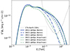 |
Fig. 8. Expected hadronic γ-ray spectra from the molecular cloud DR21 considering the two possible CR distributions given by the Kraichnan (thin lines) and Bohm (thick lines) cases. The spectra are calculated considering different relative distances from Cyg OB2: 40 pc (solid line), 60 pc (dashed line), and 80 pc (dot-dashed line). The dotted line shows the CTA North point source sensitivity for 50 h of exposure considering the Alpha Configuration. |
7. Conclusions
Young massive star clusters probably represent a population of galactic CR sources that can accelerate particles up to very high energies, generating sizeable extended γ-ray emission. In order to assess their properties as accelerators, an accurate study of this emission is needed, with robust modelling of the CR propagation in their neighbourhood. In the present paper, we consider the specific case of Cygnus OB2, which is associated with extended γ-ray emission, as observed by several experiments, from a few GeVs up to hundreds of TeVs. We studied this emission under the assumption that it is purely hadronic and produced by CRs accelerated at the TS of the cluster wind (Morlino et al. 2021). In our model, the spectral and morphological properties of the emission depend on several properties of the system: the wind luminosity, Lw, the target density ngas, the diffusion coefficient, D, and the particle acceleration efficiency, ϵcr. For the latter, the only diagnostic is to compare the computed and observed emission, and ϵcr can only be estimated at the end of our calculation, once meaningful estimates of the other parameters have been input.
To constrain the wind luminosity, we studied the stellar population of Cyg OB2 and, based on empirical relations for the properties of stellar wind, we infer a range of Lw ∈ [1.5 − 2.9]×1038 erg s−1. To estimate the gas density we used the column density of neutral atomic and molecular gas, being the ionized component negligible. We have obtained ngas ≃ 8.5 cm−3.
Finally, the type of diffusion is a crucial ingredient, as it regulates the maximum energy, the shape of the cut-off, and the CR spatial profile. The diffusion properties depend on the level of magnetic turbulence in the wind-blown bubble. We assume that turbulence is produced by MHD instabilities that convert a fraction of ηB ∼ 0.1 of the wind luminosity into magnetic fields. The turbulence power spectrum is unknown, and therefore we decided to explore three different models commonly adopted in the astrophysics literature: Kolmogorov, Kraichnan, and Bohm.
From the spectral analysis of the observed γ-ray emission, we rule out the Kolmogorov case, as the wind luminosity needed to reproduce the spectrum is Lw ≳ 5 × 1039 erg s−1, which is more than one order of magnitude higher than that inferred from the stellar population study. Likewise, also the Kraichnan model requires a high wind luminosity to reproduce the observed flux. However, if the value of ηB is increased up to ∼0.3 (a rather extreme but not impossible value), the γ-ray emission can still be reproduced. Differently from the Kolmogorov and Kraichnan cases, Bohm-like turbulence, being more efficient at scattering particles, guarantees better confinement and requires a much smaller CR luminosity of the wind. Hence, the γ-ray spectrum can be explained assuming a standard value of Lw = 2 × 1038 erg s−1 and a lower efficiency in generating magnetic field (i.e. ϵcr = 2.2% and ηB = 2.4 × 10⁻³ instead of ϵcr = 13% and ηB = 0.1). The spectral analysis alone is insufficient to discriminate between the Kraichnan and Bohm cases, as both models can provide a reasonable fit of the observed data. There is also the possibility that the actual diffusion is something in between the Bohm and the Kraichnan type. Numerical MHD simulation could in principle shed light on this point.
From our study of the γ-ray emission morphology, we find that the projected profile in all cases is almost constant in radius, which is consistent with HAWC observations. A flat profile is also expected in the Fermi-LAT domain. Nevertheless, in this case, the results are in contrast with the analysis of Fermi-LAT data by Aharonian et al. (2019), which shows a centrally peaked morphology. Such a morphology is indeed expected in a diffusion-dominated regime, but we show that it is unlikely to be realised in the region close to YMSC where strong winds are present, resulting in an advection-dominated regime, especially for low-energy particles. A possible explanation of the observed centrally peaked morphology in the Fermi-LAT energy range could be related to particle acceleration taking place in the cluster core; perhaps in the wind–wind collision regions.
At present, the γ-ray morphology and spectrum do not allow us to discriminate between Kraichnan and Bohm transport; however, this may become possible with upcoming new data and experiments, as discussed in Sect. 6.2. While X-ray data by e-Rosita could provide useful constraints by shedding light on the bubble structure, the most promising direct diagnostic for CR acceleration comes from high-spatial-resolution γ-ray observations, which could show emission from the molecular clouds in the cluster vicinity or spectral variation of the emission with distance from the cluster core. These will be possible with CTA and ASTRI-MiniArray.
In this work, we neglect a possible contribution from leptonic emission. The main reason behind this choice is that a dominant leptonic contribution to VHE γ-ray emission is disfavoured by several pieces of evidence analysed in recent works (Guevel et al. 2023; Neronov et al. 2023). In addition to this, we show in Sect. 6.3 that electrons accelerated at the wind TS cannot reach energies much larger than ∼100 TeV, implying that they cannot produce the highest energy photons detected by LHAASO. A possible leptonic contribution at lower energy remains possible, but requires an unusually high electron acceleration efficiency (see Sect. 6.3). Better quantification of the extent to which – and where in the spectrum – leptons can contribute to the γ-ray emission of Cyg-OB2 will be the subject of a forthcoming article.
The results obtained in this work rely on the assumption that the age of Cyg OB2 is 3 Myr. As reported in Sect. 2, Wright et al. (2015) estimate an age range of 3 − 5 Myr. If the age of Cyg OB2 is 5 Myr, the energy injected by supernova explosions should be of the same order as that of stellar winds (see Appendix B). In such a scenario, our model for particle acceleration should be revised to account for the CR acceleration at SNR shocks (Vieu et al. 2022a), which will likely dominate the CR production. However, this requires a detailed description of the SNR–wind bubble interaction able to account for all the relevant physical ingredients, which is not a straightforward task. Further work in this direction is necessary. In any case, we note that there are presently no clear signatures of SN explosions in Cyg OB2.
The assumed density is typical of giant molecular clouds, as shown in the analysis by Menchiari (2023).
In the numerical approach by Blasi & Morlino (2023) the 1D transport Eq. (8) is discretised and solved numerically on a grid. The main advantage of that approach is that it allows one to deal with any radial dependence of the fluid velocity downstream of the TS, while the analytical solution presented by Morlino et al. (2021) is only valid for u ∝ r−2.
We recall that pmax, as defined here, is not the actual maximum momentum of the system, which is determined by the combination of both the diffusion length upstream and downstream (see Morlino et al. 2021).
The collaboration recently posted a new preprint (Lhaaso 2024) but spectral data points and corresponding errors are not provided, and therefore we cannot properly include them in our analysis.
Acknowledgments
This work has been partially funded by the European Union – Next Generation EU, through PRIN-MUR 2022TJW4EJ. We also acknowledge the support by INAF through grant PRIN INAF 2019 “From massive stars to supernovae and supernova remnants: driving mass, energy and cosmic rays in our Galaxy”. S.M. and G.M. are partially supported by INAF through Theory Grant 2022 “Star Clusters As Cosmic Ray Factories” and Mini Grant 2023 “Probing Young Massive Stellar Cluster as Cosmic Ray Factories”.
References
- Abdollahi, S., Acero, F., Ackermann, M., et al. 2020, ApJS, 247, 33 [Google Scholar]
- Abeysekara, A. U., Albert, A., Alfaro, R., et al. 2021, Nat. Astron., 5, 465 [NASA ADS] [CrossRef] [Google Scholar]
- Abramowski, A., Acero, F., Aharonian, F., et al. 2012, A&A, 537, A114 [NASA ADS] [CrossRef] [EDP Sciences] [Google Scholar]
- Ackermann, M., Ajello, M., Allafort, A., et al. 2011, Science, 334, 1103 [NASA ADS] [CrossRef] [Google Scholar]
- Aguilar, M., Aisa, D., Alpat, B., et al. 2015, PRL, 114, 171103 [NASA ADS] [CrossRef] [Google Scholar]
- Aharonian, F. A. 2004, Very High Energy Cosmic Gamma Radiation : a Crucial Window on the Extreme Universe (World Scientific Publishing Co. Pte. Ltd.) [CrossRef] [Google Scholar]
- Aharonian, F., Yang, R., & de Oña Wilhelmi, E. 2019, Nat. Astron., 3, 561 [Google Scholar]
- Aharonian, F., Ashkar, H., Backes, M., et al. 2022, A&A, 666, A124 [NASA ADS] [CrossRef] [EDP Sciences] [Google Scholar]
- Albacete-Colombo, J. F., Drake, J. J., Flaccomio, E., et al. 2023, ApJS, 269, 14 [NASA ADS] [CrossRef] [Google Scholar]
- Astiasarain, X., Tibaldo, L., Martin, P., Knödlseder, J., & Remy, Q. 2023, A&A, 671, A47 [NASA ADS] [CrossRef] [EDP Sciences] [Google Scholar]
- Baade, W., & Zwicky, F. 1934, Phys. Rev., 46, 76 [NASA ADS] [CrossRef] [Google Scholar]
- Bartoli, B., Bernardini, P., Bi, X. J., et al. 2014, ApJ, 790, 152 [NASA ADS] [CrossRef] [Google Scholar]
- Bell, A. R., Schure, K. M., Reville, B., & Giacinti, G. 2013, MNRAS, 431, 415 [Google Scholar]
- Berlanas, S. R., Wright, N. J., Herrero, A., Drew, J. E., & Lennon, D. J. 2019, MNRAS, 484, 1838 [NASA ADS] [Google Scholar]
- Binns, W., Wiedenbeck, M., Arnould, M., et al. 2008, New Astron. Rev., 52, 427 [CrossRef] [Google Scholar]
- Blasi, P., & Morlino, G. 2023, MNRAS, 523, 4015 [CrossRef] [Google Scholar]
- Bolton, J. G. 1948, Nature, 162, 141 [NASA ADS] [CrossRef] [Google Scholar]
- Buzzoni, A. 2002, AJ, 123, 1188 [Google Scholar]
- Bykov, A. M., Marcowith, A., Amato, E., et al. 2020, Space. Sci. Rev., 216, 42 [NASA ADS] [CrossRef] [Google Scholar]
- Cao, Z., Aharonian, F. A., An, Q., et al. 2021, Nature, 594, 33 [NASA ADS] [CrossRef] [Google Scholar]
- Cardillo, M., Amato, E., & Blasi, P. 2015, Astropart. Phys., 69, 1 [Google Scholar]
- Carroll, B. W., & Ostlie, D. A. 1996, An Introduction to Modern Astrophysics (Cambridge University Press) [Google Scholar]
- Casse, M., & Paul, J. A. 1980, ApJ, 237, 236 [CrossRef] [Google Scholar]
- Castor, J., McCray, R., & Weaver, R. 1975, ApJ, 200, L107 [NASA ADS] [CrossRef] [Google Scholar]
- Cesarsky, C. J., & Montmerle, T. 1983, Space Sci. Rev., 36, 173 [NASA ADS] [CrossRef] [Google Scholar]
- Comerón, F., & Pasquali, A. 2012, A&A, 543, A101 [NASA ADS] [CrossRef] [EDP Sciences] [Google Scholar]
- Cristofari, P., Blasi, P., & Caprioli, D. 2022, ApJ, 930, 28 [NASA ADS] [CrossRef] [Google Scholar]
- Dame, T. M., Hartmann, D., & Thaddeus, P. 2001, ApJ, 547, 792 [Google Scholar]
- Demircan, O., & Kahraman, G. 1991, Ap&SS, 181, 313 [Google Scholar]
- Dickel, H. R., Wendker, H., & Bieritz, J. H. 1969, A&A, 1, 270 [NASA ADS] [Google Scholar]
- Downes, D., & Rinehart, R. 1966, ApJ, 144, 937 [Google Scholar]
- Draine, B. T. 2011, Physics of the Interstellar and Intergalactic Medium (Princeton University Press) [Google Scholar]
- Drew, J. E., Greimel, R., Irwin, M. J., & Sale, S. E. 2008, MNRAS, 386, 1761 [Google Scholar]
- Drury, L. O. 1983, Rep. Prog. Phys., 46, 973 [Google Scholar]
- Dwarkadas, V. V. 2023, Galaxies, 11, 78 [NASA ADS] [CrossRef] [Google Scholar]
- Eker, Z., Bakış, V., Bilir, S., et al. 2018, MNRAS, 479, 5491 [NASA ADS] [CrossRef] [Google Scholar]
- El-Badry, K., Ostriker, E. C., Kim, C.-G., Quataert, E., & Weisz, D. R. 2019, MNRAS, 490, 1961 [CrossRef] [Google Scholar]
- Emig, K. L., White, G. J., Salas, P., et al. 2022, A&A, 664, A88 [NASA ADS] [CrossRef] [EDP Sciences] [Google Scholar]
- Funk, S. 2017, in Handbook of Supernovae, eds. A. W. Alsabti, & P. Murdin, 1737 [CrossRef] [Google Scholar]
- Green, G. M., Schlafly, E., Zucker, C., Speagle, J. S., & Finkbeiner, D. 2019, ApJ, 887, 93 [NASA ADS] [CrossRef] [Google Scholar]
- Guevel, D., Beardmore, A., Page, K. L., et al. 2023, ApJ, 950, 116 [CrossRef] [Google Scholar]
- Gupta, S., Nath, B. B., Sharma, P., & Eichler, D. 2020, MNRAS, 493, 3159 [CrossRef] [Google Scholar]
- Haggerty, C. C., & Caprioli, D. 2020, ApJ, 905, 1 [Google Scholar]
- Hanson, M. M. 2003, ApJ, 597, 957 [NASA ADS] [CrossRef] [Google Scholar]
- Helder, E. A., Vink, J., Bykov, A. M., et al. 2012, Space. Sci. Rev., 173, 369 [NASA ADS] [CrossRef] [Google Scholar]
- Hey, J. S., Parsons, S. J., & Phillips, J. W. 1946, Nature, 158, 234 [NASA ADS] [CrossRef] [Google Scholar]
- Johnson, H. L., & Morgan, W. W. 1954, ApJ, 119, 344 [NASA ADS] [CrossRef] [Google Scholar]
- Kafexhiu, E., Aharonian, F., Taylor, A. M., & Vila, G. S. 2014, Phys. Rev. D, 90, 123014 [Google Scholar]
- Kaur, H., Sharma, S., Dewangan, L. K., et al. 2020, ApJ, 896, 29 [NASA ADS] [CrossRef] [Google Scholar]
- Kelner, S. R., Aharonian, F. A., & Bugayov, V. V. 2006, Phys. Rev. D, 74, 034018 [Google Scholar]
- Khangulyan, D., Aharonian, F. A., & Kelner, S. R. 2014, ApJ, 783, 100 [Google Scholar]
- Kiminki, D. C., Kobulnicky, H. A., Vargas Álvarez, C. A., Alexander, M. J., & Lundquist, M. J. 2015, ApJ, 811, 85 [NASA ADS] [CrossRef] [Google Scholar]
- Knödlseder, J. 2000, A&A, 360, 539 [NASA ADS] [Google Scholar]
- Koyama, K., Petre, R., Gotthelf, E. V., et al. 1995, Nature, 378, 255 [Google Scholar]
- Kroupa, P. 2001, MNRAS, 322, 231 [NASA ADS] [CrossRef] [Google Scholar]
- Kudritzki, R.-P., & Puls, J. 2000, ARA&A, 38, 613 [Google Scholar]
- Lancaster, L., Ostriker, E. C., Kim, J.-G., & Kim, C.-G. 2021, ApJ, 914, 89 [NASA ADS] [CrossRef] [Google Scholar]
- Leitherer, C., Robert, C., & Drissen, L. 1992, ApJ, 401, 596 [Google Scholar]
- Lhaaso, C. 2024, Sci. Bull., 69, 449 [NASA ADS] [CrossRef] [Google Scholar]
- Li, C., Qiu, K., Li, D., et al. 2023, ApJ, 948, L17 [CrossRef] [Google Scholar]
- Lozinskaya, T. A., Pravdikova, V. V., & Finoguenov, A. V. 2002, Astron. Lett., 28, 223 [NASA ADS] [CrossRef] [Google Scholar]
- Massey, P., & Thompson, A. B. 1991, AJ, 101, 1408 [NASA ADS] [CrossRef] [Google Scholar]
- Menchiari, S. 2023, Ph.D. Thesis, [arXiv:2307.03477] [Google Scholar]
- Morlino, G., Blasi, P., Peretti, E., & Cristofari, P. 2021, MNRAS, 504, 6096 [NASA ADS] [CrossRef] [Google Scholar]
- Neronov, A., Semikoz, D., & Savchenko, D. 2023, arXiv e-prints [arXiv:2311.13711] [Google Scholar]
- Nieuwenhuijzen, H., & de Jager, C. 1990, A&A, 231, 134 [NASA ADS] [Google Scholar]
- Nugis, T., & Lamers, H. J. G. L. M. 2000, A&A, 360, 227 [NASA ADS] [Google Scholar]
- Orlando, S., Bocchino, F., Reale, F., Peres, G., & Pagano, P. 2008, ApJ, 678, 274 [NASA ADS] [CrossRef] [Google Scholar]
- Piddington, J. H., & Minnett, H. C. 1952, Aust. J. Sci. Res. A Phys. Sci., 5, 17 [NASA ADS] [Google Scholar]
- Prantzos, N. 2012, A&A, 538, A80 [CrossRef] [EDP Sciences] [Google Scholar]
- Reddish, V. C., Lawrence, L. C., & Pratt, N. M. 1966, Publ. R. Obs. Edinburgh, 5, 111 [NASA ADS] [Google Scholar]
- Reimer, A., Pohl, M., & Reimer, O. 2006, ApJ, 644, 1118 [NASA ADS] [CrossRef] [Google Scholar]
- Reipurth, B., & Schneider, N. 2008, in Handbook of Star Forming Regions, 4, 36 [NASA ADS] [Google Scholar]
- Renzo, M., Ott, C. D., Shore, S. N., & de Mink, S. E. 2017, A&A, 603, A118 [NASA ADS] [CrossRef] [EDP Sciences] [Google Scholar]
- Reynolds, S. P. 2008, ARA&A, 46, 89 [Google Scholar]
- Rygl, K. L. J., Brunthaler, A., Sanna, A., et al. 2012, A&A, 539, A79 [NASA ADS] [CrossRef] [EDP Sciences] [Google Scholar]
- Saha, L., Domínguez, A., Tibaldo, L., et al. 2020, ApJ, 897, 131 [NASA ADS] [CrossRef] [Google Scholar]
- Schneider, N., Bontemps, S., Simon, R., et al. 2006, A&A, 458, 855 [NASA ADS] [CrossRef] [EDP Sciences] [Google Scholar]
- Schneider, N., Csengeri, T., Bontemps, S., et al. 2010, A&A, 520, A49 [CrossRef] [EDP Sciences] [Google Scholar]
- Subedi, P., Sonsrettee, W., Blasi, P., et al. 2017, ApJ, 837, 140 [Google Scholar]
- Takekoshi, T., Fujita, S., Nishimura, A., et al. 2019, ApJ, 883, 156 [NASA ADS] [CrossRef] [Google Scholar]
- Tatischeff, V., Raymond, J. C., Duprat, J., Gabici, S., & Recchia, S. 2021, MNRAS, 508, 1321 [NASA ADS] [CrossRef] [Google Scholar]
- Taylor, A. R., Gibson, S. J., Peracaula, M., et al. 2003, AJ, 125, 20 [NASA ADS] [Google Scholar]
- Torres-Dodgen, A. V., Tapia, M., & Carroll, M. 1991, MNRAS, 249, 1 [NASA ADS] [CrossRef] [Google Scholar]
- Uyanıker, B., Fürst, E., Reich, W., Aschenbach, B., & Wielebinski, R. 2001, A&A, 371, 675 [NASA ADS] [CrossRef] [EDP Sciences] [Google Scholar]
- Vieu, T., Gabici, S., Tatischeff, V., & Ravikularaman, S. 2022a, MNRAS, 512, 1275 [NASA ADS] [CrossRef] [Google Scholar]
- Vieu, T., Reville, B., & Aharonian, F. 2022b, MNRAS, 515, 2256 [NASA ADS] [CrossRef] [Google Scholar]
- Vink, J. S., de Koter, A., & Lamers, H. J. G. L. M. 2001, A&A, 369, 574 [NASA ADS] [CrossRef] [EDP Sciences] [Google Scholar]
- Weaver, R., McCray, R., Castor, J., Shapiro, P., & Moore, R. 1977, ApJ, 218, 377 [Google Scholar]
- Weidner, C., & Kroupa, P. 2004, MNRAS, 348, 187 [NASA ADS] [CrossRef] [Google Scholar]
- Wiedenbeck, M. E., & Greiner, D. E. 1981, Phys. Rev. Lett., 46, 682 [NASA ADS] [CrossRef] [Google Scholar]
- Wilson, T. L., Rohlfs, K., & Hüttemeister, S. 2009, Tools of Radio Astronomy (Springer Berlin, Heidelberg) [Google Scholar]
- Wright, N. J., Drake, J. J., Drew, J. E., & Vink, J. S. 2010, ApJ, 713, 871 [Google Scholar]
- Wright, N. J., Drew, J. E., & Mohr-Smith, M. 2015, MNRAS, 449, 741 [NASA ADS] [CrossRef] [Google Scholar]
- Yang, R.-Z., de Oña Wilhelmi, E., & Aharonian, F. 2018, A&A, 611, A77 [NASA ADS] [CrossRef] [EDP Sciences] [Google Scholar]
- Yungelson, L. R., van den Heuvel, E. P. J., Vink, J. S., Portegies Zwart, S. F., & de Koter, A. 2008, A&A, 477, 223 [NASA ADS] [CrossRef] [EDP Sciences] [Google Scholar]
Appendix A: Estimating the cluster wind parameters from the observed stellar population
In order to calculate the total mass-loss rate and wind luminosity of Cyg OB2, one needs to compute the mass-loss rate Ṁi and the terminal wind speed v∞, i for every i-th member of the association. Both the mass-loss rate and the terminal wind speed are functions of global stellar properties: mass Mi, bolometric luminosity Li, radius R⋆, i, and Temperature Teff, i. Mass, luminosity and effective temperature (together with the associated uncertainties) are taken from the sample of stars at the core of the association by Wright et al. (2015), while to calculate the stellar radius we use the empirical relation provided by Demircan & Kahraman (1991):

The wind terminal velocity, following (Kudritzki & Puls 2000), is given by:

where 𝒞 = 2.65 for Teff, i ≥ 2.1 × 10⁴ K (Kudritzki & Puls 2000), which is adequate for the considered stellar sample,  is the escape velocity, G is the gravitational constant, and Γedd is the luminosity in units of the Eddington luminosity.
We use two different recipes to calculate Ṁi. The first one is based on a theoretical formula given by Yungelson et al. (2008)
while the second approach relies on an empirical relation for the mass-loss rate provided by Vink et al. (2001) and valid for stars with temperature 27500 K< Teff, i < 50000 K (corresponding to stars with masses larger than 20 M⊙) given by:
where Zi is the stellar metallicity (that we assume to be Solar).
In order to evaluate the reliability of our estimate of the mass-loss rate, we checked how the results depend on the approach adopted to evaluate the quantities that appear in Equation (A.4). The different approaches are the following:
-
We calculate the total mass-loss rate using Li, Teff, i, and Mi provided by Wright et al. (2015).
-
We use Li and Teff, i from Wright et al. (2015) while Mi is recomputed as Yungelson et al. (2008):
-
We use Mi and Teff, i from Wright et al. (2015) while Li is recomputed inverting Equation (A.5).
-
We take only Li from Wright et al. (2015) while Teff, i is calculated using the Boltzmann law:
and Mi is recomputed from Equation (A.5)
![$$ \begin{aligned} \frac{M_i}{{M}_\odot }=\left[ 10^{-3.48} \left( \frac{L_i}{{L}_\odot } \right) \right]^{0.75} \, . \end{aligned} $$](/articles/aa/full_html/2024/06/aa48817-23/aa48817-23-eq62.gif)
To take into account the uncertainties we use a Montecarlo approach, generating 104 different star samples where the parameters of every star have a Gaussian distribution around the mean with variance provided by Wright et al. (2015). Figure A.1 shows the result for the Ṁ calculation after considering only single stars (binary systems are not included) with Mi > 20 M⊙ and without the contribution of Wolf-Rayet (WR) stars. The value of Ṁ is found to lie in the range [0.25 × 10⁻⁴, 0.65 × 10⁻⁴] M⊙ yr−1.
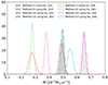 |
Fig. A.1. Mass-loss rate distribution for Cygnus OB2 considering the sample of stars investigated by Wright et al. (2015). The stellar parameters are estimated using four different recipes, from (i) to (iv), and for each one the mass-loss rate is estimated using both Equation (A.3) and (A.4). All estimates neglect the contribution due to WR stars. |
To further account for the contribution of the three Wolf-Rayet stars associated with Cyg OB2 we adopt the empirical relation by Nugis & Lamers (2000):

where both the Helium fraction (YWR, i) and metallicity (ZWR, i) are set to the Solar value. We find a contribution to the mass-loss rate from WR stars of ∼0.3 × 10⁻⁴ M⊙yr−1
The star sample of Wright et al. (2015) includes also 9 known binary systems, whose contribution to Ṁ is not straightforward to quantify. However, we can provide a rough estimate assuming that the total luminosity of the system results from two companions of equal luminosity. Then, for each of the stars, we adopt method iv described above for the calculation of Ṁi (using only Li), we find ṀBinary ∈ [0.18 ×10⁻⁴, 0.6 × 10⁻⁴]M⊙ yr−1. By summing up all the contributions, Cyg OB2 mass-loss rate should lie in a conservative range of Ṁ ∈ [0.7 × 10⁻⁴, 1.5 × 10⁻⁴]M⊙ yr−1.
Once the mass-loss rate of every star in the cluster is known, the associated wind speed is calculated from momentum conservation:
The cluster wind luminosity is then:
The contribution of single, non WR stars, accounting for both the values of Ṁi inferred using the theoretical and empirical recipes of Yungelson et al. (2008) and Vink et al. (2001), is in the range ![$ L_{\mathrm{w}}^{\mathrm{nbs}} \in [0.4\times 10^{38}, 1.6 \times 10^{38}] $](/articles/aa/full_html/2024/06/aa48817-23/aa48817-23-eq67.gif) erg s−1 (see Figure A.2). The wind luminosity contribution from the three Wolf-Rayet stars included in the sample of Wright et al. (2015) (assuming an average wind speed of 2000 km s−1 is
erg s−1 (see Figure A.2). The wind luminosity contribution from the three Wolf-Rayet stars included in the sample of Wright et al. (2015) (assuming an average wind speed of 2000 km s−1 is  erg s−1. Finally, the contribution of the 9 binary systems is
 ![$ L_{\mathrm{w}}^{\mathrm{bs}} \in [0.55\times 10^{38}, \, 0.7 \times 10^{38}] $](/articles/aa/full_html/2024/06/aa48817-23/aa48817-23-eq69.gif) erg s−1. Accounting for all contributions, Cyg OB2 wind luminosity should lie in the range Lw ∈ [1.55 × 1038, 2.9 × 1038] erg s−1.
erg s−1. Accounting for all contributions, Cyg OB2 wind luminosity should lie in the range Lw ∈ [1.55 × 1038, 2.9 × 1038] erg s−1.
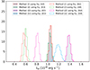 |
Fig. A.2. Wind luminosity of Cygnus OB2 inferred using the estimated mass-loss rates (see text). |
It is worth noticing that our estimate is compatible with the results of other works where different approaches have been used. For example, Lozinskaya et al. (2002) used the total mass of the association and the average wind luminosity per solar mass provided by Leitherer et al. (1992), obtaining Lw ≃ 1 × 1039 erg s−1. However this value is likely overestimated as it is based on the stellar population study done by Knödlseder (2000), which likely overestimated the number of stars. Following the same approach and rescaling the mass to that measured by Wright et al. (2015), the expected wind luminosity is ∼3.3 × 1038 erg s−1. Similarly, Ackermann et al. (2011) evaluate a wind luminosity of Lw ∈ [2 × 1038, 3 × 1038] erg s−1 considering a different sample of stars that includes the presence of 17 stars with M⋆ > 35 M⊙ and 5 Wolf-Rayet. Finally, in a recent analysis of the diffuse X-ray emission, Albacete-Colombo et al. (2023) provide an estimate of the total wind luminosity of ≈1.5 × 1038 erg s−1.
Appendix B: Estimating the cluster wind parameters from the stellar IMF
An alternative approach to estimate the cluster wind parameters based only on the cluster stellar mass and age was presented by Menchiari (2023). This approach is especially useful if the stellar population is not known. The method can be summarised as follows: knowing the cluster mass, a mock stellar population is simulated by random sampling an assumed initial mass function. Afterward, given the age of the cluster, all stars massive enough to have exploded as supernova are removed from the population. The cluster wind properties are then calculated after estimating the wind parameters for all the mock stars. This method can be used to cross check the results obtained in Appendix A for the main sequence stars, with the additional advantage that we can estimate the number of supernovae exploded within the cluster. The latter is useful to understand whether the energetics of the bubble is dominated by winds or rather by supernovae explosions. Finally, we apply this alternative method to NGC 6910.
We here assume the initial mass function by Kroupa (2001), which is suitable for Cyg OB2 (Wright et al. 2015). Stars are sampled in the mass range between M⋆, min = 0.08 M⊙ and M⋆, max = 150 M⊙. The lower limit on the mass range is associated with the minimum mass required to start hydrogen nuclear burning (Carroll & Ostlie 1996), while the maximum mass is an empirical upper limit fixed by observations (Weidner & Kroupa 2004). Being ξ⋆(M⋆) the initial mass function, the total number of stars in the cluster and the cluster mass are:
Once the initial stellar population has been generated, all stars that have left the main sequence are removed from the sample (i.e. we neglect any evolutionary phase out of the main sequence), assuming the turnover time (tTO) for a star of mass M⋆, given by (Buzzoni 2002):

For a given stellar mass we set the luminosity through the mass-luminosity relation presented in Menchiari (2023). This consists of a smoothed broken power law joining two different empirical mass-luminosity relations: the first one provided by Eker et al. (2018) and valid between 0.179–31 M⊙, and the second one provided by Yungelson et al. (2008) and valid for very massive stars (M⋆ ≳ 35 M⊙):
![$$ \begin{aligned} L_\star = {\left\{ \begin{array}{ll} L_{\rm b1} \left(\frac{M_\star }{M_{\rm b1}} \right)^{\alpha _1} \left[ \frac{1}{2}+ \frac{1}{2} \left( \frac{M_\star }{M_{\rm b1}} \right)^{1/\Delta _1}\right]^{(-\alpha _1+\alpha _2)\Delta _1} \\ \text{ for} 2.4 \le \frac{M_\star }{{M}_\odot } < 12 \\ L_{\rm b2} \left(\frac{M_\star }{M_{\rm b2}} \right)^{\alpha _2} \left[ \frac{1}{2}+ \frac{1}{2} \left( \frac{M_\star }{M_{\rm b2}} \right)^{1/\Delta _2}\right]^{(-\alpha _2+\alpha _3)\Delta _2} \\ \text{ for} M_\star \ge 12 \textit{M}_\odot \end{array}\right.} \end{aligned} $$](/articles/aa/full_html/2024/06/aa48817-23/aa48817-23-eq73.gif)
where Lb1 = 3191 L⊙, Lb2 = 301370 L⊙, Mb1 = 7 M⊙ and Mb2 = 36.089 M⊙. The value of Mb2 is the intersection point between the two mass luminosity relations of Yungelson et al. (2008) and Eker et al. (2018). The power law indexes are α1 = 3.97, α2 = 2.86, and α3 = 1.34. The parameters Δ1 and Δ2 are used to smooth the transition between the different power law components. We fix the two parameters to 0.01 and 0.15, respectively. We note that in the interval 2.4–12 M⊙ the mass luminosity relation is taken from Eker et al. (2018) and adapted so as to ensure continuity at Mb1 = 7 M⊙.
To calculate the stellar radius, we use the same relation (A.1) adopted in Appendix A. Given that the mock stellar population includes also stars with masses below 20 M⊙, to calculate the mass-loss rate, we use the empirical relation by Nieuwenhuijzen & de Jager (1990):
which is valid for stars with temperatures above 5000 K, (Ṁ⋆ ≳ 3 M⊙). To this purpose, when calculating the wind properties we only account for stars with M⋆ > 3 M⊙, corresponding to O and B type stars. The contribution to the wind power and mass-loss rate for stars with lower masses is totally negligible (Menchiari 2023).
Once the parameters of each single star are known, the stellar wind power and velocity are calculated using Equations (A.2) and (A.8). The collective cluster wind power and mass-loss rate are then calculated by summing up all the contributions of the mock stars.
Cyg OB2 has a total stellar mass of  M⊙ and an age between 3-5 Myr (Wright et al. 2015). Assuming an age of 3 Myr, after simulating 103 different mock stellar populations, we found an average wind luminosity and mass-loss rate of Lw = 0.8 × 1038 erg s−1 and Ṁ = 0.3 × 10⁻⁴ M⊙ yr−1 (see Figure B.1), which are consistent with the estimates obtained in Appendix A, neglecting WR stars. Moreover, as emphasised by Berlanas et al. (2019), 10% of the stellar mass of Cyg OB2 is likely associated with a foreground OB association. By rescaling the mass accordingly, the wind luminosity and mass-loss rate values change by only ∼10%, and are therefore consistent with the estimates provided in Appendix A.
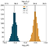 |
Fig. B.1. Distribution of wind luminosity (left side histogram) and mass-loss rate (right side histogram) of Cygnus OB2 inferred using a montecarlo method based on a mock stellar population. The values are obtained after generating 1000 different stellar populations. The dashed and solid lines represent the average wind luminosity and mass-loss rate, respectively. |
One can wonder how the power injected by possible SNe compares to that of the wind. The above procedure can also be used to estimate the number of SNe exploded in the cluster by counting how many massive stars have a main sequence phase lasting less than the cluster age. For ∼3 Myr the expected number of supernova is 7 ± 2.5. Assuming that each SN releases an energy of 1051 erg, the total is ∼7 × 1051 erg, a factor ∼2.5 smaller than the total energy injected by the stellar winds. The latter can be found by integrating in time the cluster wind luminosity, and is ∼1.8 × 1052 erg. We, hence, expect that the bubble dynamics and particle acceleration process is still dominated by the power of stellar winds. However, this is not true anymore if the age of Cyg OB2 is ∼5 Myr. In such a case, the expected number of SNe rises to 26 ± 5, resulting into total power slightly larger than the wind power. For the sake of completeness, we also mention that from an observational point of view there are no clear indications of the presence of recent SN explosions.
Finally, as mentioned in the Introduction, close to Cyg OB2 there is a second cluster, NGC 6910. By using the same method described above we can calculate its wind luminosity. The cluster has an estimated age of ∼4.5 Myr and a lower limit to the mass of ∼775 M⊙ (Kaur et al. 2020). NGC 6910 is also characterised by an initial mass function scaling as to  (Kaur et al. 2020), harder than the one by Kroupa (2001). Using these values we get an average wind luminosity and mass-loss rate of Lw = 1.8 × 1036 erg s−1 and Ṁ = 7.6 × 10⁻⁷ M⊙ yr−1. The expected number of supernovae is, instead, ∼4 ± 2. Even doubling the value of the estimated cluster mass, the final luminosity of NGC 6910 will remain negligible compared to Cyg OB2.
All Tables
Best-fit parameters values and main system properties for three different models.
All Figures
|
Fig. 1. Multi wavelength view of the Cygnus-X star forming region. Upper panel: combination of observations at 500 μm and 8 μm from the Herschel SPIRE and MSX telescopes of the Cygnus X star-forming complex. Radiation at 500 μm (light blue scale) indicates emission from cold dust, while the 8 μm (orange scale) traces photon-dominated regions. Lower panel: continuum observations at 1.42 GHz from the Canadian Galactic Plane Survey (Taylor et al. 2003). A large fraction of this emission is likely thermal free-free radiation by material possibly ionised by Cyg OB2 (Emig et al. 2022). Colour scales are given in arbitrary units. |
| In the text | |
|
Fig. 2. Radial CR distribution normalised to its value at the termination shock in the case of Kolmogorov (top panel), Kraichnan (central panel), and Bohm (bottom panel) turbulence. In these plots, the contribution of the Galactic CR sea to fcr has not been included. |
| In the text | |
|
Fig. 3. Gas column and number density in the vicinity of Cyg OB2. Top panel: total target column density considering the ISM in the neutral and molecular phases. The column density of HI has been evaluated using the 21 cm line observation from the CGPS, while for the molecular gas, we used a combination of 12CO observations from the Nobeyama radio telescope and the data from the 12CO galactic plane survey by Dame et al. (2001). All the observations are kinematically cut selecting only the gas between −20 and 20 km s−1. White rings represent the regions used by Aharonian et al. (2019) and Abeysekara et al. (2021) to probe the γ-ray radial profile. The radii of the different circles correspond to angular sizes of 0.61°, 1.19°, 1.8° and 2.21°. Bottom panel: average gas density profile in the Cygnus region for each annulus. |
| In the text | |
|
Fig. 4. Spectral energy distribution of the expected hadronic γ-ray emission extracted from a region of 2.2° centred on Cyg OB2. Lines in different panels refer to Kolmogorov (top panel), Kraichnan (middle panel), and Bohm cases (bottom panel). Solid lines always represent the best-fit curves, whose underlying parameters are summarised in Table 2. Other line-types correspond to the values of the parameters listed in the legend inside each panel. |
| In the text | |
|
Fig. 5. Comparison with observations of the expected γ-ray surface brightness radial profile for the Kraichnan (upper panel) and Bohm (bottom panel) cases. Black squares correspond to the measurements by Fermi-LAT (Aharonian et al. 2019), while purple circles indicate the surface brightness observed by HAWC (Abeysekara et al. 2021). Grey squares represent Fermi-LAT measurements rescaled by a factor of 2. Diamonds and crosses indicate the surface brightness values based on our model, at energies of 10 < Eγ < 316 GeV and 1 < Eγ < 251 TeV respectively. |
| In the text | |
|
Fig. 6. Comparison between diffusion (thin lines) and advection (thick lines) timescales for the Kraichnan (green dashed lines) and Bohm (blue solid lines) cases. The black dotted line shows the diffusion time in the case of a diffusion coefficient with the same slope as that in the standard interstellar medium normalised a factor of 100. All timescales are calculated considering only the region used for the morphological analysis, i.e. substituting Rb with 54 pc in Eqs. (20) and (21). |
| In the text | |
|
Fig. 7. Expected hadronic γ-ray spectra extracted from rings at projected distances of |
| In the text | |
|
Fig. 8. Expected hadronic γ-ray spectra from the molecular cloud DR21 considering the two possible CR distributions given by the Kraichnan (thin lines) and Bohm (thick lines) cases. The spectra are calculated considering different relative distances from Cyg OB2: 40 pc (solid line), 60 pc (dashed line), and 80 pc (dot-dashed line). The dotted line shows the CTA North point source sensitivity for 50 h of exposure considering the Alpha Configuration. |
| In the text | |
|
Fig. A.1. Mass-loss rate distribution for Cygnus OB2 considering the sample of stars investigated by Wright et al. (2015). The stellar parameters are estimated using four different recipes, from (i) to (iv), and for each one the mass-loss rate is estimated using both Equation (A.3) and (A.4). All estimates neglect the contribution due to WR stars. |
| In the text | |
|
Fig. A.2. Wind luminosity of Cygnus OB2 inferred using the estimated mass-loss rates (see text). |
| In the text | |
|
Fig. B.1. Distribution of wind luminosity (left side histogram) and mass-loss rate (right side histogram) of Cygnus OB2 inferred using a montecarlo method based on a mock stellar population. The values are obtained after generating 1000 different stellar populations. The dashed and solid lines represent the average wind luminosity and mass-loss rate, respectively. |
| In the text | |
Current usage metrics show cumulative count of Article Views (full-text article views including HTML views, PDF and ePub downloads, according to the available data) and Abstracts Views on Vision4Press platform.
Data correspond to usage on the plateform after 2015. The current usage metrics is available 48-96 hours after online publication and is updated daily on week days.
Initial download of the metrics may take a while.