© The Authors 2024

1 Introduction

GRAVITY+ (GRAVITY+ Collaboration 2022) is a combined upgrade of the GRAVITY instrument and of its host observatory the Very Large Telescope Interferometer (VLTI, GRAVITY Collaboration 2017) of the European Southern Observatory (ESO). Among other work packages, it features a major update of its adaptive optics (AO) systems, with a renewal of all the instances installed on each of the four unit telescopes (UTs) of the VLTI.

The role of an AO system is to compensate in real time for the wavefront aberrations induced by atmospheric turbulence (Roddier 1999). These phase aberrations are measured by a wavefront sensor (WFS) whose signals are analysed by a real time computer (RTC) and turned into a set of commands sent to a deformable mirror (DM) that compensates the optical aberrations. To be effective, this feedback loop must run faster than the turbulence temporal evolution, with typical frequencies ranging from several hundred Hertz to a kilo-Hertz.

In the case of the GRAVITY+ adaptive optics (GPAO, Le Bouquin 2023), the RTC is based on the upgrade of the Standard Platform for Adaptive optics Real Time Applications (SPARTA-upgrade, Suárez Valles et al. 2012; Shchekaturov 2023; Dembet 2023) which inherits the high level functionalities developed for the Spectro Polarimetric High-contrast Exoplanet REsearcher (SPHERE, Beuzit et al. 2019) and the Adaptive Optics Facility (AOF, Oberti et al. 2018). Overall, GPAO features a 43×43 DM with about 1200 actuators within the 100 mm pupil and Shack-Hartmann wavefront sensors (SH-WFSs, Shack & Platt 1971): a 30×30 laser guide star (LGS) WFS, and a variety of natural guide stars (NGS) WFSs (visible 40×40, visible 4×4, infrared 9×9). The pupil of the system is given by the secondary mirror (M2) of the telescope, defining the beam size and position. The DM is located in the Coudé train of the telescope, rotating with the azimuth, while the WFSs are at the Coudé focus, fixed to the ground. Moreover, a number of sub-system within the AO WFS have to also track the azimuth and/or the elevation angles (a K-mirror, an atmospheric dispersion compensator, and the table used to patrol the field). The elevation and the azimuth rotations of the telescope itself have wobble amplitude of 2% of the pupil diameter. The tracking sub-systems within the WFS have typical wobble amplitude of 5% of the pupil diameter. As a consequence of this configuration, for the most resolving SH-WFS (40×40), the combined wobble amplitude corresponds to several subapertures.

This significant wobbling of the system leads to two important requirements for GPAO: (I) GPAO needs a means to quickly estimate large lateral-registration during the acquisition of the target to within an accuracy to achieve stable closed loop operation, controlling most of the observable modes (typically 20% of the subaperture size, see for instance Oberti et al. 2016); (II) during the subsequent observation, the azimuth and elevation angle continues to evolve, and so do their intrinsic wobbles, and GPAO needs a mean to track this small and continuously changing lateral-registration, while the AO loop is closed. However, because the DM is not the instrument pupil, the imprint of the photometric pupil in the WFS cannot be used to track this lateral-registration, as is typically done in most AO systems. This is even more applicable when the system operates on the internal light source of the VLTI, which does not properly define a photometric pupil because of its location at the Nasmyth focus (i.e. after M2). Therefore, there is a need for a proper, direct measurement of the DM/WFS lateral-registration at a level of 20% of the sub-aperture diameter at instrument preset and through operation.

One complete instance of GPAO out of the four is currently being integrated and tested at the Lagrange laboratory in Nice (Millour et al. 2022). The test bench features multiple sources, a turbulent phase screen, a pupil mask mimicking the VLT, and a beam expander to properly illuminate the DM and the SH-WFSs with the correct beam size and f-number. The bench permits operation of GPAO in both NGS and LGS modes, with the caveat that the LGS source does not incorporate spot elongation and cone effect. The results presented in this paper focus on the NGS VIS WFS (40×40, point source) mode but all tests have also been performed with the LGS WFS as well (30×30, extended source).

Regarding the mis-registration errors, the registration of a couple DM/WFS is defined by how the actuator geometry of the former is seen by the optics geometry of the latter¹. This global geometry is defined in the design phase of the instrument. A mis-registration error occurs when there is a mismatch between the designed values and the real system. Among others (Heritier 2019, Sect. 2.1), the classical (and most impacting) misregistrations are the x and y-shifts (lateral translation of the DM with respect to the WFS), the clocking (rotation of the DM with respect to the WFS), and the magnification and anamorphosis (stretches of the DM with respect to the WFS).

Different techniques exist to assess the mis-registration state of an AO system. For instance, in the case where the DM is also the pupil of the instrument, the WFS photometry can be used to track the lateral error (Kolb 2016). However, most of the tools to track mis-registrations use the interaction matrix (IM) of the AO system (Roddier 1999). Close to its functioning point, an AO system is assumed to be linear and the IM links the commands sent to the DM to the measures provided by the WFS². If the AO system is sensitive to the considered mis-registration, an alignment error should then leave a signature in its IM.

In early AO systems, with a limited number of actuators and with an internal calibration source providing high signal-to-noise ratios (S/Ns), IMs were experimentally measured and the AO systems were run with ‘as-built’, rather than ‘as-designed’ IMs (Oberti et al. 2006). Doing so, any mis-registration error is calibrated and taken into account by the AO loop. The arrival of telescopes with adaptive secondary mirrors, such as the Multiple Mirror Telescope (Brusa et al. 2003), the Large Binocular Telescope (Riccardi et al. 2003), or the AOF (Ströbele et al. 2006), complicated the identification of registration errors. Indeed, without any focal plane available upstream of the DM, and thus no reference source, the AO system must be calibrated directly on-sky at night. Different techniques to measure the full IM were implemented, such as fast ‘push-pull’ commands to freeze the turbulence or command modulation and signal demodulation to increase the S/N (Oberti et al. 2006; Pinna et al. 2012; Lai et al. 2021). But such IMs are generally noisy and depend on the experimental conditions (Kolb 2016). In addition, night time is precious and the increase of AO system complexity is synonymous to longer and more sensitive calibrations.

To tackle these issues, new methods emerged, based on the fact that a physical modelling of the interaction matrix is generally available, so-called synthetic IM (Oberti et al. 2006; Heritier et al. 2018a). By definition, these matrices are noiseless but sensitive to model errors, that is to say a mismatch between the numerical model and the real system (Kolb et al. 2012). If the first order of WFS physics is correctly implemented, the misregistrations become this main source of error (Heritier 2019) and the synthetic model thus only depends on a limited number of parameters. These parameters can be fitted through calibrations to obtain pseudo-synthetic interaction matrices (PSIMs), where the ‘pseudo’ emphasises that inputs from the real system are used in the synthetic model (Oberti et al. 2006).

In general, the parameter fitting is performed on IMs acquired for this purpose during dedicated calibration procedures, on internal sources or on-sky (Oberti et al. 2004; Neichel et al. 2012; Kolb 2016; Heritier et al. 2018a). Nonetheless, misregistrations are susceptible to evolve during observation due to mechanical flexion or thermal evolution. And future Extremely Large Telescopes (ELTs, Johns 2006; Gilmozzi & Spyromilio 2007; Boyer 2018) will bring this challenge to another level, with unprecedented distances between DMs and WFSs, with potentially different moving/rotating parts in-between, prone to misalignment. It then becomes impossible to perform regular calibrations and it is thus necessary to track the evolution of the mis-registrations directly during the scientific acquisitions with online tools for AO system auto-calibration. A strategy that has proven to be effective is recovering the IM directly from AO telemetry data (Béchet et al. 2012; Kolb et al. 2012). These methods introduced the fact that the measurement noise propagates through the AO loop, producing meaningful signal from which the IM can be estimated. Nonetheless, a large amount of telemetry data must be gathered so that the IM structure emerges from the loop noise, strongly increasing the recording and computation times. In addition, Heritier (2019, Sect. 4.3) showed that such an approach can be corrupted by the temporal error of the AO loop, with a bias induced by a frozen flow turbulence.

To further save time while increasing the S/N and debiasing the error estimation, recent works have started to focus on partial IM acquisition, focussing on dedicated and well chosen modes injected in the AO loop (Heritier et al. 2021). Contrary to online IM estimation, this method is invasive and may corrupt the science depending on the chosen modes and the amplitude to apply to get meaningful S/N. A trade-off must be balanced, for example, by applying the disturbance during the shutter closing time of the science instrument if possible. Such an invasive method is the current baseline of the AO systems of the first generation of instruments of the ESO ELT.

Finally, all these methods are based on the minimisation of the difference between the measured IM and the PSIM. Such PSIM models are generally complex and not directly invertible. Under the assumption that the mis-registration errors are small, the PSIMs are linearised close to their functioning point to get sensitivity matrices, leading to an iterative fit of the parameters, potentially laborious and slow and with a limited capture range (Kolb et al. 2012; Neichel et al. 2012; Heritier et al. 2018a). There have been several variants or improvements of this technique in recent years. Heritier (2019, Sect. 2.5.4) recomputes iteratively the sensitivity matrix in order to increase the capture range and achieve a larger linearity. Heritier et al. (2021) performed a numerical demonstration that such modal IMs, and thus the misregistrations, can be estimated in a closed loop with a dedicated perturbation in the command, while controlling the linearity sensitivity of the estimator; however the applicability of this method in the lab or on-sky is yet to be confirmed.

To meet the two requirements of GPAO introduced above: (1) there is still a lack of a fast and robust method with a large capture range and that works in open loop to quickly align the system at preset and during science target acquisition; and (2) during operation, we still miss a fast³ and non-invasive tool to monitor the lateral error, with the additional constraints that the solutions must be adaptable to the SPARTA architecture. To answer these two requirements, we present (in Sects. 2 and 3 of this paper) two new methods to fit the lateral errors in the system. The first one is based on a perturbative approach, whereby two-dimensional (2D) modes are applied on the system in open loop in order to be spatially correlated to a reference. The second one is a non-perturbative approach working in closed loop by analysing correlation signals in the telemetry of the commands.

We present the methods in Sects. 2.1 and 3.1. For each method, (i) its general idea is given; (ii) then its theoretical steps are developed; and (iii) finally, we summarise its main advantages. Then, in Sects. 2.2 and 3.2, we assess the precision and the limits of the methods via end-to-end simulations. Finally, in Sects. 2.3 and 3.3, we validate our approaches on a real system in the GPAO development bench.

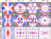Fig. 1 General idea of the spatial 2D correlation method for different KL modes mKL ∈ {6, 20, 35, 46}. When different modes are applied on the DM (first line), the patterns seen by the WFS show different spatial scales (second line). The grey pixels correspond to the missing slopes wWFS (x) = 0 in the PSIM model that are hidden by the pupil. A lateral mis-registration would shift the peak in the correlation between the PSIM and the measured IM (third line).

2 Perturbative 2D modal estimator

2.1 Proposed method

2.1.1 General concept

A SH-WFS produces spatial measurements of the input wave-front’s gradient. Thus, when a spatial pattern is applied on the DM, a specific spatial pattern will be seen in the SH-WFS data. The pattern applied on the DM can be its individual influence functions (zonal IM) or dedicated modes such as Zernike polynomials or Karhunen–Loève (KL) functions (Dai 1995) obtained by combining DM commands (modal IM). Figure 1 presents some KL modes applied in the DM space (first line) and their counter-part on the x-slopes of the SH-WFS (second line) when reshaped in 2D. As expected, the patterns in the 2D representation of SH-WFS slopes are highly structured with a pattern specific to each mode.

The idea of the proposed method is to use IMs that are Nyquist-sampled, in the sense that the highest spatial frequency in the generated gradients is sampled by at least two subapertures. In this case, a lateral mis-registration in the system can be approximated by a, possibly sub-subaperture, geometric shift of the measurements. Thus, the 2D spatial correlation of a measured modal IM with a reference modal IM should be usable as a lateral error estimator. Contrary to other solutions based on modal perturbations, such as the one proposed by Heritier et al. (2021), this method does not use a synthetic IM model fitting that implies the tuning of its parameters, but it uses the 2D representation of the measured IMs to directly estimate the parameters of interest.

Nonetheless, as seen in the auto-correlation of the KL modes in Fig. 1 (third line), the sensitivity of the correlation to a misalignment will depend on the considered mode, as already mentioned by Heritier et al. (2021). Low spatial frequency modes, such as m^KL = 6, produce a single but extended correlation peak while high spatial frequency modes, such as m^KL = 35, produce localised but multiple correlation peaks. By working with different modes, our method aims at combining the large capture range of the low spatial frequencies with the sensitivity of the high spatial frequencies. The only constrain is to use KL modes whose gradients are properly sampled by the WFS.

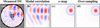Fig. 2 Simulated example of the spatial 2D correlation method. Panel a: simulation of a measured and shifted modal IM (x-slopes) for mKL = 35. The grey and dark pixels correspond to the non-valid slopes wvalid(x) = 0 in the measured IM. Panel b: cross-correlation of the shifted mode of Panel a with the reference modal IM for mKL = 35 (see Fig. 1). Panel c: map of the fitted coefficients α. Panel d: over-sampling of panel c with an interpolation via sinc functions.

2.1.2 Estimation of the registration error from a modal IM

As explained in the previous section, the method implies to reshape the slopes of the modal IM on 2D spatial positions x = (x, y) lying on a 2D Cartesian grid of pitch Δ, the subaperture size. Nonetheless, on such a square grid, some slopes are missing in the model (pupil external edge and central obscuration by the secondary mirror) and are set to zero. They are highlighted in grey in Fig. 1. In the following, we note this mask of modelled slopes: $$w^{\mathrm{W}\mathrm{F}\mathrm{S}}(x)=\{\begin{array}{l}1\text{ if the slope at }x\text{ is in the IM, }\\ 0\text{ otherwise. }\end{array}$$(1)

On top of the slopes outside the pupil, partially illuminated subapertures of the SH-WFS, noisier than the others, are invalidated and considered as missing data. In the following, we note this mask of valid slopes: $$w^{\text{valid }}(x)=\{\begin{array}{l}1\text{ if the slope at }x\text{ is valid, }\\ 0\text{ otherwise. }\end{array}$$(2)

As emphasised in black in Fig. 2a and compared to the modelled slopes in Fig. 1, this corresponds to an additional missing ring of one subaperture width on the outer ring and the corners of the inner ring of the pupil.

In the following, we note ${\mathit{M}}_m^{\mathrm{i}\mathrm{n}\mathrm{t}}(\mathit{x})(\text{ resp. }{\tilde{\mathit{M}}}_m^{\mathrm{i}\mathrm{n}\mathrm{t}}(\mathit{x}))$ the reference modal IM of the system without any mis-registration (resp. the measured modal IM). Here, x is the 2D position in terms of subaperture of the SH-WFS and m is the index of the considered mode. The reference IM can be an IM measured during calibration on a well-aligned system, relaxing the need of a synthetic IM. For GPAO, we chose to use a synthetic IM which is computed once for all.

For a given mode m, the cross-correlation of the 2D IMs is given by: $$[{\tilde{\mathit{M}}}_m^{\mathrm{i}\mathrm{n}\mathrm{t}}⊛{\mathit{M}}_m^{\mathrm{i}\mathrm{n}\mathrm{t}}](\mathit{\delta })\triangleq {\displaystyle \sum _{\mathit{x}}}{\tilde{\mathit{M}}}_m^{\mathrm{i}\mathrm{n}\mathrm{t}}(\mathit{x}){\mathit{M}}_m^{\mathrm{i}\mathrm{n}\mathrm{t}}(\mathit{x}-\mathit{\delta })=\alpha (\mathit{\delta }).$$(3)

In terms of δ, Eq. (3) would give maps similar to the third line of Fig. 1 or Fig. 2b. These maps can quickly be obtained by performing the cross-correlation in the Fourier space. Then, finding the value of δ maximising this correlation α(δ) could give a hint on the lateral error. Nonetheless, as discussed above, the sensitivity of this solution will depend on the chosen mode m and this modal estimator does not provide a natural way to combine the different modes into a single general estimator. In addition, such a cross-correlation assumes that all the summed 2D positions x are relevant. It does not account for the valid subapertures in the model nor in the measures via Eqs. (1) and (2). As a consequence, this will strongly bias the estimated error in case of large mis-registrations due to pupil truncation effects.

In our method, we rather define α(δ) in terms of how similar the two IMs are in terms of mean squares, jointly accounting for all the modes, $$\alpha (\mathit{\delta })=\underset{\beta }{\mathrm{argmin}}{\displaystyle \sum _{\mathit{x}\mathbf{,}\mathit{m}}}w(\mathit{x},\mathit{\delta }){({\tilde{\mathit{M}}}_m^{\mathrm{i}\mathrm{n}\mathrm{t}}(\mathit{x})-\beta {\mathit{M}}_m^{\mathrm{i}\mathrm{n}\mathrm{t}}(\mathit{x}-\mathit{\delta }))}^2,$$(4)

with: $$w(\mathit{x},\mathit{\delta })=w^{\text{valid }}(\mathit{x})w^{\mathrm{W}\mathrm{F}\mathrm{S}}(\mathit{x}-\mathit{\delta }).$$(5)

The weight factor w(x, δ) discards from the cost function the invalid pairs $[{\tilde{\mathit{M}}}_m^{\mathrm{i}\mathrm{n}\mathrm{t}}(\mathit{x}),{\mathit{M}}_m^{\mathrm{i}\mathrm{n}\mathrm{t}}(\mathit{x}-\mathit{\delta })]$ if one of the elements is estimated on an invalid position. Equation (4) has an analytical solution given by $$\alpha (\mathit{\delta })=\frac{\sum _{\mathit{x}\mathbf{,}\mathit{m}}w(\mathit{x},\mathit{\delta }){\tilde{\mathit{M}}}_m^{\mathrm{i}\mathrm{n}\mathrm{t}}(\mathit{x}){\mathit{M}}_m^{\mathrm{i}\mathrm{n}\mathrm{t}}(\mathit{x}-\mathit{\delta })}{\sum _{\mathit{x}\mathbf{,}\mathit{m}}w(\mathit{x},\mathit{\delta }){[{\mathit{M}}_m^{\mathrm{i}\mathrm{n}\mathrm{t}}(\mathit{x}-\mathit{\delta })]}^2},$$(6) $$=\frac{\sum _m[w^{\mathrm{v}\mathrm{a}\mathrm{l}\mathrm{i}\mathrm{d}}{\tilde{\mathit{M}}}_m^{\mathrm{i}\mathrm{n}\mathrm{t}}⊛w^{\mathrm{W}\mathrm{F}\mathrm{S}}{\mathit{M}}_m^{\mathrm{i}\mathrm{n}\mathrm{t}}](\mathit{\delta })}{\sum _m[w^{\mathrm{v}\mathrm{a}\mathrm{l}\mathrm{i}\mathrm{d}}⊛w^{\mathrm{W}\mathrm{F}\mathrm{S}}{\left[{\mathit{M}}_m^{\mathrm{i}\mathrm{n}\mathrm{t}}\right]}^2](\mathit{\delta })}.$$(7)

Thus, the coefficient map α(δ) is expressed by the ratio of the modal sum of 2D cross-correlations.

To achieve super-resolution without the need of a complex model fitting method, this low resolution map α(δ) is further up-sampled by zero-padding its Fourier transform by a factor m^up = 8. This factor ensures a resolution of 12.5% of a subaperture, finer than the target error of 20% mentioned in Sect. 1. This step does not add any information, but it is equivalent to an interpolation with a sinc function, oversampling the maximum region with a continuous function. Other methods involving polynomial fit or an iterative weighted center of gravity could be used but slower and prone to converge to local maxima. On the contrary, using a zero-padding operation is numerical very efficient, and handle all maxima at once. In the end, the position of the global maximum of the obtained map gives the estimated lateral mis-registration $\tilde{\mathit{\delta }}$ at the resolution given by the up-sampling parameter m^up in a single pass: $$\tilde{\mathit{\delta }}=\underset{\mathit{\delta }}{\mathrm{argmax}}\alpha (\mathit{\delta }).$$(8)

Looking closer at the definition of α in Eq. (4), it appears that $\alpha (\tilde{\mathit{\delta }})$ gives the optimal coefficient to maximise the similarity between ${\mathit{M}}_m^{\mathrm{i}\mathrm{n}\mathrm{t}}$ and ${\tilde{\mathit{M}}}_m^{\text{int }}$ in the sense of the mean squares. In other words, $\alpha (\tilde{\mathit{\delta }})$ gives the correction to apply on the amplitude of the guessed PSIM to obtain the real global amplitude of the measured IM.

In the following, we pragmatically chose to use the set of the 50 first KL modes. As discussed in Sec. 4.1 and Appendix A, it was beyond the scope of this paper to further optimise the considered modes. The chosen option produces a modal base that can be shared with all the GPAO modes (9×9, 30×30 and 40×40 SH-WFS). In the following, we work within the framework of the 40×40 SH-WFS GPAO mode.

2.1.3 Advantages of the spatial correlation estimator

Here, we list the main advantages of the proposed method. First, by accounting for the valid subapertures with an appropriate map Eq. (1), this method is robust to large errors and strongly misaligned systems. It has a large capture range because of the exhaustive exploration of the parameter space permitted by Eq. (8). The estimator is absolute. It provides unbiased and super-resolved measures, up to the resolution of the up-sampling parameter m^up.

Afterwards, the application of the method is fast: by focussing only on a limited numbers of modes, the acquisition of the modal IM is quick to obtain. And it is fast to compute: the convolutions in Eq. (7), with proper zero-padding, can be computed using fast 2D discrete Fourier transforms and the fit of the lateral error is obtained in a single pass via Eq. (8). Thus, there is no need to recompute several PSIM to iterate the parameter fit.

Furthermore, the need of a PSIM model is reduced to the minimal need: a single computation to get the reference IM from which the command matrix of the AO loop is derived. For complex systems where a PSIM model is not available, this need could be removed by using a measured IM obtained during calibration on an aligned system.

Because it is based on lots of redundant measures to retrieve only the two parameters of the lateral error, the proposed estimator has a high S/N. This makes it particularly suitable for open-loop calibration where the turbulence strongly corrupts the slopes of the measured modal IM, as far as the measurement strategy freezes, in average, the turbulence (Kolb 2016). In addition, Heritier et al. (2021) has shown that these kinds of approaches are not biaised by the turbulence wind.

Finally, an interesting by-product of the method is the global amplitude of the IM, which is given by the amplitude of the correlation peak. Although this does not provide the individual amplitude on each actuator of the DM, this is an interesting parameter for the monitoring and re-calibration of the system and its AO loop. Even if this beyond the scope of this paper which focuses on SH-WFS, we also notice here that estimating the amplitude of the IM could be trickier with a pyramid WFS as the optical gains will vary with the considered modes. This would change their relative weighting in Eq. (7), but should not modify the definition of the best position.

2.2 Simulations: large capture range

The modal correlation estimator was tested with the AOF tool embedded in SPARTA in charge of generating PSIMs. As described by Kolb et al. (2012), it uses a geometrical model of the SH-WFS. The slopes are obtained by computing the wavefront phase difference on the opposite edges of each subaperture. For the DM, we used a pseudo-synthetic model. For each actuator a of the ALPAO DM, its influence function ψ_a is described with a symmetrically radial profile: $${\psi }_a(x)=A_a.{\mathrm{e}}^{-{\alpha }_a{\left(|x|/{\mathrm{\Delta }}^{\mathrm{D}\mathrm{M}}\right)}^{\beta a}},$$(9)

where Δ^DM is the actuator pitch, where A_a is the amplitude of the actuator, and where α_a and β_a = are the parameters of the super-Gaussian profile. The values of these parameters are fitted on the real influence functions measured and kindly provided by ALPAO. The actuator positions and influence functions are stretched according the GPAO design⁴ and consequently do not lie on a Fried geometry (Fried 1977). The KL modes are defined on the actuator command space, following the covariance method described by Bertrou-Cantou et al. (2022).

To test the method, a zonal PSIM was generated with extreme lateral registration error of δ = (δ_x, δ_y) = (13.35, 8.65)δ and an amplitude of 4 μm for the DM actuators in the visible NGS mode of GPAO (40×40 SH-WFS). Noisy measurements were simulated by adding a centered Gaussian noise on the slopes with a standard deviation of σ^slope = 0.25 pixel, corresponding to a noise of 200 mas in the GPAO design. Results are shown in Fig. 2, using KL modes from m^KL = 4 to m^{KL, max} = 50.

Figure 2a shows the m^KL = 35^th mode of the modal IM obtained after projecting the zonal IM on the KL modes. Compared with its centered representation in Fig. 1, the introduced shift is visible with a slope pattern clearly off-centered from the WFS pupil. In addition, it appears that the noise on the zonal IM propagates towards the modal IM. For information, the correlation of this shifted noisy pattern with its reference is given in Fig. 2b. The results is smooth, but finding the position of the maximal correlation is ambiguous with several potential locations (red regions).

This ambiguity is lifted when looking at the map of the fitted coefficients α in Fig. 2c. Only one clear location emerges for the maximal correlation. The noise on this map is negligible and its oversampled version of Fig. 2d leads to an estimated shift of $\tilde{\mathit{\delta }}$ = (13.375, 8.625)Δ and an amplitude of 3.99 μm. The results is in the resolution of 1/m^up = 0.125 of a subaperture. The amplitude is also correctly estimated, within a percent.

For information, the impact of the number of modes on the estimator performances is briefly discussed in Appendix A. As studied in Appendix B.1, the cross-talk with other misregistration parameters (rotation and magnification) is negligible for realistic cases.

2.3 Experimental results: System alignment at preset

The 2D modal estimator was tested in the GPAO development bench. To show that the method does not rely on a Fried geometry, an angle of 35° was applied between the DM pupil and the WFS pupil. The wind was emulated by spinning the phase plate at its maximal speed. This produces a wind of υ₀ ≃ 8.4 m s⁻¹ with a Fried parameter of r₀ ≃ 14 cm. The WFS stage was translated by several subapertures, as illustrated in Fig. 3a. A few iterations of the lateral error corrective loop were performed with a gain of 0.8 as shown in Fig. 4. To freeze the turbulence, the modal IMs were measured with the fast ‘push-pull’ method (Kasper et al. 2004; Oberti et al. 2006; Kolb 2016), playing sequentially the different modes. The AO loop was open.

Qualitatively speaking, the shift of the pupil in Fig. 3a is clearly visible in the modal IM of Fig. 3c despite the high level of noise. The under-illumination threshold of SPARTA automatically sets the slopes of poorly illuminated subapertures to zero. The over-sampled map of Fig. 3d has a clear optimal area.

The corrective loop converges in only three iterations, as seen in Fig. 4. The period of the iteration is dominated by the overhead times of SPARTA when measuring the IM and the time to move the actuator of the translating stage. The time to actually poke the DM is 10 ms per mode, so half a second, and the time to correlated the measured IM with the model is negligible. After the alignment, the noisy pattern of the modal IM of Fig. 3e, convingly matches the reference pattern of Fig. 3f. Furthermore, it can be seen from Fig. 3b that the photometric pupil of the system is off-centred⁵. Some subapertures do not get flux despite being in the SH-WFS pupil (top-left) while some others outside the pupil are illuminated (bottom-right). This supports the fact that except for a rough alignment of the system, the photometric pupil cannot be used to align the DM actuator geometry and the SH-WFS.

To quantitatively assess the alignment efficiency, interaction matrices were measured prior and after the system auto-alignment. For these measurements, the phase plate was stopped to prevent any bias. SPARTA embeds an AOF tool to estimate the mis-registration parameters of the system by PSIM iterative model fitting, as described by Kolb et al. (2012). The results are presented in Table 1.

The initial lateral error is δ = (−908.5, −377.4)%Δ. From Fig. 4, with the phase plate spinning, the error initially found by the 2D modal estimator is $\tilde{\mathit{\delta }}$ = (−937.5, −400.0)%Δ. Remembering that m^up = 8, this estimation lies within three resolution elements of 12.5%Δ of the up-sampled map α. This is thus better than half a subaperture and despite the fact that the system presents a magnification of ~ 1%, not considered in the estimator. After convergence $(\tilde{\mathit{\delta }}=\mathbf{0})$, Table 1 shows that the actual lateral misalignment is well below the up-sampled map α resolution, with a residual of a few percent of a subaperture.

At convergence, the amplitude fitted by the 2D modal estimator is 3.4 μm. If this is the correct order of magnitude, it is ~13% below the amplitude given by the SPARTA fit given in Table 1. Several factors can explain this discrepancy. First, the IM is measured by playing a Hadamard set of zonal commands (Kasper et al. 2004; Oberti et al. 2004), producing potentially strong local slopes on the DM and thus not the same linearity point of the system than the one of the modal IM measurement. In addition, the |δ_ρ| ≃ 1.5% stretch in the system measured by SPARTA is not included in the reference IM of the estimator. This can further bias the model fitting of Eq. (8). Better understanding this amplitude was not considered critical in this study. This is indeed an interesting by-product of the method, but we mainly wanted to focus on the system auto-alignment.

Finally and importantly, we remark here that the precision of the alignment obtained with the 2D modal estimator is sufficient to close the AO loop with an IM and a control matrix synthesised for a perfectly aligned system (δ = 0) and controlling 500 modes, which corresponds to the baseline of GPAO for standard operation. This shows that the 2D modal estimator is a robust tool to put the system in state where the closed loop estimator presented hereafter can take over the lateral misalignment monitoring and correction.

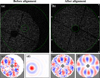Fig. 3 Example in the GPAO bench of the 2D modal estimator. Panels a, b: SH-WFS pixels before and after the alignment. Green circles: WFS pupil edges. Panels c, e, f: x-slopes of the modal IM for mKL = 40 before (panel c) and after (panel e) alignment and reference (panel f). panel d: over-sampled map of the coefficient α before alignment.

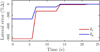Fig. 4 Convergence of the lateral error corrective loop with the 2D modal estimator at GPAO preset.

3 Non-perturbative closed loop estimator

3.1 Proposed method

3.1.1 Block diagram of an AO loop

A standard AO loop works as follows. First, the WFS S converts the 2D wavefront w into measurements m corrupted by noise, n: $$\mathit{m}=S(\mathit{w})+\mathit{n}.$$(10)

Next, these measurements are processed by the controller C to compute a new command to send to the DM: $$\mathit{c}=C(\mathit{m}).$$(11)

Then, this command is applied and held by the DM until the next command arrives. For example, in the case of GRAVITY+, m are slopes delivered by the SH-WFS and the controller is a leaky integrator⁶ of leak gain g^ε and integral gain g^∫: $${\mathit{c}}^{i+1}=(1-g^{ϵ}){\mathit{c}}^i+g^{\int }{\mathit{c}}^{\delta },$$(12)

and where the command correction: $${\mathit{c}}^{\delta }={\mathit{M}}^{\mathrm{c}\mathrm{m}\mathrm{d}}\mathit{m},$$(13)

is obtained with a command matrix M^cmd computed by inverting the PSIM of the system filtered on a given n^mod number of KL modes.

In the following, we work under different assumptions. Firstly, when an AO system is in closed loop, it can be linearised around its operating point, and all the previously described steps become linear operations. It is then equivalent to describe the AO loop in the Fourier space of the commands m and of the wavefront w that is to say in terms of 2D spatial frequencies k = (k_x, k_y) (m⁻¹) propagating through the system. Secondly, in such a system, without any misalignment (no lateral shift, no clocking and no stretch between the sensor and the actuators), there is no cross-coupling between different 2D spatial frequencies k ≠ k′. For a spatial frequency k, the above steps (i), (ii), and (iii) can then be represented by the block diagram of Fig. 5 where each block is a linear operation. The symmetric (equivalently the real part of the Fourier coefficient) and the anti-symmetric part (equivalently the imaginary part of the Fourier coefficient) of this spatial frequency are presented with the subscripts one (blue) and two (green).

The effect of the different blocks of Fig. 5 can be described by their transfer function defined in the temporal frequency space f (Hz) (Åström & Murray 2021). It is a reasonable assumption to consider that the transfer functions are identical for the two spatial modes: $$\{\begin{array}{l}{S}_1=S_2=S,\\ C_1=C_2=C,\\ A_1=A_2=A.\end{array}$$(14)

As detailed by Madec (1999), the WFS integrates the signal during its exposure time τ^WFS giving the transfer function: $$S(f)=\frac{1-{\mathrm{e}}^{-2i\pi {\tau }^{\mathrm{W}\mathrm{F}\mathrm{S}}f}}{2i\pi {\tau }^{\mathrm{W}\mathrm{F}\mathrm{S}}f}.$$(15)

Then, C is a leaky controller of transfer function: $$C(f)=\frac{g^{\int }{\mathrm{e}}^{-2i\pi {\tau }^{\mathrm{l}\mathrm{a}\mathrm{t}}f}}{1-(1-g^{ϵ}){\mathrm{e}}^{-2i\pi {\tau }^{\mathrm{R}\mathrm{T}\mathrm{C}}f}},$$(16)

where τ^lat is the latency of the system (communication and computation times) and τ^RTC is the period of the RTC cycle⁷. Finally, the DM acts as a zero-controller holder, maintaining the command during τ^DM with a transfer function similar to the WFS: $$A(f)=\frac{1-{\mathrm{e}}^{-2i\pi {\tau }^{\mathrm{D}\mathrm{M}}f}}{2i\pi {\tau }^{\mathrm{D}\mathrm{M}}f}.$$(17)

In general, all the characteristic times are equal: $${\tau }^{\text{lat }}\simeq {\tau }^{\mathrm{D}\mathrm{M}}\simeq {\tau }^{\mathrm{W}\mathrm{F}\mathrm{S}}\simeq {\tau }^{\mathrm{R}\mathrm{T}\mathrm{C}}.$$(18)

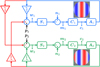Fig. 5 Block diagram of the temporal coupling (in red) of the symmetric (cosine, in blue) and anti-symmetric (sine, in green) parts of a given spatial frequency k = (2/3D, 0) through the AO loop.

3.1.2 Temporal coupling of a 2D spatial frequency

In the following, x = (x, y) denotes for the 2D spatial position. Using the notations of Fig. 5, a lateral 2D shift δ = (δ_x, δ_y) between the DM and the WFS implies a spatial phase shift between the spatial frequency k of the wavefront w seen by the WFS and its correction c by the DM as follows: $$\{\begin{array}{ll}(1)& {\mathit{c}}_1\propto \cos (2\pi {\mathit{k}}^T\cdot \mathit{x})\Rightarrow \mathit{w}\propto -\cos (2\pi {\mathit{k}}^T\cdot (\mathit{x}-\mathit{\delta })),\\ (2)& {\mathit{c}}_2\propto \sin (2\pi {\mathit{k}}^T\cdot \mathit{x})\Rightarrow \mathit{w}\propto -\sin (2\pi {\mathit{k}}^T\cdot (\mathit{x}-\mathit{\delta })).\end{array}$$(19) $$\{\begin{array}{ll}(1)& \mathit{w}\propto -\cos (\theta )\cos (2\pi {\mathit{k}}^T\cdot \mathit{x})-\sin (\theta )\sin (2\pi {\mathit{k}}^T\cdot \mathit{x}),\\ & \mathit{w}\propto -\cos (\theta ){\mathit{w}}_1-\sin (\theta ){\mathit{w}}_2,\\ (2)& \mathit{w}\propto +\sin (\theta )\cos (2\pi {\mathit{k}}^T\cdot \mathit{x})-\cos (\theta )\sin (2\pi {\mathit{k}}^T\cdot \mathit{x}),\\ & \mathit{w}\propto +\sin (\theta ){\mathit{w}}_1-\cos (\theta ){\mathit{w}}_2,\end{array}$$(20)

with the coupling coefficient of: $$\theta =2\pi {\mathit{k}}^T\cdot \mathit{\delta }.$$(21)

As emphasised by the red arrows in Fig. 5, there is now consequently a cross-coupling between the symmetric (1) and anti-symmetric (2) parts of the spatial frequency k.

The commands c₁ and c₂ are thus no longer independent. Discussing on the noise propagation through an AO loop, Heritier (2019, Sect. 4.1.3) already mentioned the fact that measurement noise can produce signals and intuited that the larger the mis-registration, the higher the S/N on the measures would be. The present method is based on the fact that such a coupling between c₁ and c₂ leaves a trace in their temporal correlation. In the (spatial and temporal) Fourier space, the variance of the command c_i(k, f) of a given spatial frequency k at a temporal frequency f is defined by: $${\mathcal{V}}_{c_i}(\mathit{k},f)\triangleq ⟨c_i(\mathit{k},f){\overline{c}}_i(\mathit{k},f)⟩,$$(22)

and the correlation between c₁ and c₂ for this given spatial frequency k at the temporal frequency f is defined by: $${\mathcal{C}}_{{\mathit{c}}_1,{\mathit{c}}_2}(\mathit{k},f)\triangleq \frac{⟨c_1(\mathit{k},f){\overline{c}}_2(\mathit{k},f)⟩}{\sqrt{{\mathcal{V}}_{c_1}(\mathit{k},f){\mathcal{V}}_{c_2}(\mathit{k},f)}}.$$(23)

Under the assumption that the different noise terms n_i and p_i are independent, we show in Appendix C that the coupling of c₁ and c₂ through the system produces a signature in their correlation that only depends on the coefficient θ and the frequency f. This signature is expressed by: $${\mathcal{C}}_{{\mathit{c}}_1,{\mathit{c}}_2}(\theta (\mathit{k}),f)/\theta (\mathit{k})\underset{\theta \to 0}{\sim }2i\mathcal{I}\left[\frac{\overline{\mu }(f)}{1+\overline{\mu }(f)}\right]\triangleq i{\mathcal{C}}_0(f),$$(24)

with: $$\mu \triangleq ACS.$$(25)

The correlation of a given spatial frequency k is thus a pure imaginary number. Figure 6 shows the imaginary parts of the correlation ${\mathcal{C}}_{c_1,c_2}$ (θ, f) for different values of the coupling coefficient θ.

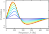Fig. 6 Imaginary part of the correlation curves ${\mathcal{C}}_{c_1,c_2}$ (θ, f) in a noise limited regime for various values of θ from 0° (blue) to 45° (red), every 5°. AO parameters: τWFS = 1 ms, g∫ = 0.5, gε = 0.

3.1.3 Estimation of the registration error from telemetry

First, to apply the results of Sect. 3.1.2, the spatio-temporal cube of commands c(x, t) recorded in the closed loop telemetry must be reshaped in terms of spatial and temporal frequencies and split on its symmetric and anti-symmetric compounds. With the notation of Fig. 5, this 3D cube can be written as: $$c(\mathit{x},t)={\displaystyle \sum _{\mathit{k}}}{c}_1(\mathit{k},t)\cos (2\pi {\mathit{k}}^T\cdot \mathit{x})+c_2(\mathit{k},t)\sin (2\pi {\mathit{k}}^T\cdot \mathit{x}).$$(26)

with: $$c_1(-\mathit{k},t)=c_1(\mathit{k},t)\text{ and }{c}_2(-\mathit{k},t)=-c_2(\mathit{k},t)\text{, }$$(27)

to ensure the parity of the symmetric and anti-symmetric parts c₁ and c₂. As a consequence, the discrete 3D Fourier transform of c, ℱ(k, f), is equal to: $${\mathcal{F}}_c(\mathit{k},f)=c_1(\mathit{k},f)-i{c}_2(\mathit{k},f),$$(28)

and thus: $$\{\begin{array}{l}{c}_1(\mathit{k},f)=\frac{1}{2}[{\mathcal{F}}_c(\mathit{k},f)+{\mathcal{F}}_c(-\mathit{k},f)],\\ c_2(\mathit{k},f)=\frac{i}{2}[{\mathcal{F}}_c(\mathit{k},f)-{\mathcal{F}}_c(-\mathit{k},f)].\end{array}$$(29)

Then, the imaginary part of the empirical correlation of the closed loop telemetry is computed as follows: $${\tilde{\mathcal{C}}}^{\mathrm{c}\mathrm{l}}(\mathit{k},f)=\mathcal{I}\left[\frac{c_1(\mathit{k},f){\overline{c}}_2(\mathit{k},f)}{|c_1(\mathit{k},f)||c_2(\mathit{k},f)|}\right].$$(30)

The control space k ∈ $\mathcal{K}$^ctrl of the AO loop is delimited by a disk of radius k^max, in terms of cycle per diameter, so that: $$\pi {\left[k^{\mathrm{m}\mathrm{a}\mathrm{x}}\right]}^2=\frac{n^{\mathrm{m}\mathrm{o}\mathrm{d}}}{n^{\text{act }}}{\left[d^{\mathrm{a}\mathrm{c}\mathrm{t}}\right]}^2,$$(31)

where d^act is the number of actuators across the diameter of the telescope and n^act is the total number of actuators of the DM. Equation (31) states that among the [d^act]² modes in the Cartesian Fourier space, only the ratio of the number of controlled modes n^mod over the maximal number of degree of freedom are controlled. We thus get from Eqs. (21) and (24) that: $$\mathbf{\forall }\mathit{k}\in {\mathit{K}}^{\mathrm{c}\mathrm{t}\mathrm{r}\mathrm{l}},{\tilde{\mathcal{C}}}^{\mathrm{c}\mathrm{l}}(\mathit{k},f)\simeq 2\pi {\mathcal{C}}_0(f){\mathit{k}}^T\cdot \mathit{\delta }.$$(32)

Finally, the lateral error is given by: $$\tilde{\mathit{\delta }}=\underset{\delta }{\mathrm{argmin}}{\displaystyle \sum _{\mathit{k}\in {\mathcal{K}}^{\mathrm{c}\mathrm{t}\mathrm{r}\text{l}},f>0}}{({\tilde{\mathcal{C}}}^{\mathrm{c}\mathrm{l}}(\mathit{k},f)-2\pi {\mathcal{C}}_0(f){\mathit{k}}^T\cdot \mathit{\delta })}^2.$$(33)

This problem is solved by expanding the dimensions along k and f in order to reshape the equation into a matrix-vector shape, $${\tilde{\mathcal{C}}}^{\mathrm{c}\mathrm{l}}(\mathit{k},f)\simeq H(\mathit{k},f)\times \mathit{\delta },$$(34)

and using the pseudo-inverse H^† of the obtained matrix (Moore 1920; Penrose 1955), $$\tilde{\mathit{\delta }}=[H(\mathit{k},f){]}^{†}\times {\tilde{\mathcal{C}}}^{\mathrm{c}\mathrm{l}}(\mathit{k},f).$$(35)

3.1.4 Advantages of the closed loop estimator

As discussed below, the proposed method has numerous advantages. Firstly, it is purely based on the geometry of the chosen observable which can be the WFS measurements m_i or the DM commands c_i. It only uses the history of this observable and its correlation. Knowing explicitly the link between WFS measurements and the DM commands is not needed. Thus, the method does not rely on any PSIM model from which mis-registration parameters must be retrieved and the method is consequently not prone to model errors. In addition, such PSIM models are generally complex (and potentially non-invertible) and extremely slow to compute, strongly slowing the iterative fit of the alignment errors. Secondly, the model only depends on only a small number of parameters driving the AO loop. These parameters are generally well constrained by design or proper calibration.

Furthermore, the estimator, expressed in the Fourier domain, is sparse. This makes it extremely fast to compute, a critical aspect when considering the ever increasing number of actuators and system complexity of the future ELTs.

Even if it based on noise propagation, assumptions on the noise model remain minimal. The method only supposes that the noise is spatially uncorrelated, but for a given spatial frequency, it does not assume a specific noise model. If white noises n_i would excite all the spatial and temporal frequencies and thus produce a strong signal in the command correlation, knowing the power spectrum density of the noise sources is not needed as it cancels out via Eq. (23), as shown in Appendix C.

Finally, a common issue with lateral error estimators based on the AO telemetry is their sensitivity to the wind in the case of a frozen flow turbulence (Heritier et al. 2019; Heritier 2019). As discussed in Appendix C.2, such a situation breaks the assumption that p₁ and p₂ are independent, used to get Eq. (24). Nonetheless, as far as there is noise injected in the loop to produce a correlation signal in the commands, this effect is sparse in the temporal frequency space. Thus, compared to other methods based on AO loop telemetry (Béchet et al. 2012; Kolb et al. 2012), the wind should have a limited impact on the proposed estimator of Eq. (33).

3.2 Simulations: Sensitivity and wind bias

3.2.1 End-to-end simulations

We used an ideal model for the DM. The influence functions ψ_a = ψ were set to be identical for all actuators a by replacing the parameters in Eq. (9) by their median value fitted on the ALPAO DM: A_a = 9 μm, α_a = 0.87 and β_a = 1.31. For a null lateral error, the actuators were placed on a 41×41 grid (d^act = 41) in a Fried geometry (Fried 1977) leading to n^act = 1353 active actuators. Thus the DM pitch Δ^DM is also equal to the size of a subaperture Δ. To introduce a minimal control on loop divergence, the commands are clipped between minus one and one.

A purely geometrical model was used to simulate the SH-WFS. The slopes were estimated by averaging the gradient obtained by finite difference in each subaperture of the SH-WFS at the wavelength λ^wfs = 750 nm. There is no diffractive propagation of the wavefront to produce spot and consequently no spot centroiding. Only the photon shot noise was considered and added directly to the geometrical slopes, using Eq. (D.4) as detailed in Appendix D.

Table 2 sums up the different notations used in Sects. 3.2 and 3.3. The sensitivity of the estimator to some of these parameters, especially the wind speed υ₀ and the noise level n^ph, is studied in the following, only focussing on the lateral error δ introduced in the system. Cross-talk with other mis-registration is discussed in Appendix B.2.

3.2.2 Sensitivity of the closed loop estimator

The sensitivity of the closed loop estimator was assessed by injecting known lateral errors δ^th in the system, with amplitudes ranging from |δ^th| = 0% to 70% of a subaperture pitch Λ every 5% and angles ranging from $\mathcal{A}$[δ^th] = 0° to 355° every 5°. For each case, batches of 500 consecutive closed loop iterations in a pure noise regime wihtout any turbulence were gathered for different numbers of controlled modes. The estimated lateral errors $\tilde{\mathit{\delta }}$ were de-rotated with the known angles $\mathcal{A}$[δ^th] to compute its mean value and its standard deviation for each amplitude |δ^th|. The results are shown in Figs. 7 and 8.

From Fig. 7, it appears that the estimator follows a linear law for errors lower than 25% of Δ for n^mod ≤ 800. As expected, the more modes are used and the less noisy is the estimator. Nonetheless, the linearity range decreases with the number of modes, suggesting limitation in the approximation of Eq. (24). Indeed, estimating the lateral error via Eq. (33) does not solve the inverse problem of Eq. (C.13) but its Taylor expansion of Eq. (C.14) for negligible coefficients θ ~ 0. As the correlation curves depend on this coefficient, see Fig. 6, this can bias the estimator. The saturation of the estimator and the associated increase of its standard deviation for n^mod ≥ 500 and for |δ^th| > 50% are linked with the limit of stability of the loop at large mis-registrations. This leads to DM command clipping and thus non-linearities in the system. This limit is reached at a smaller lateral error of |δ^th| = 20% when controlling an extreme number of modes of n^mod = 1200.

Surprisingly, the sensitivity of the estimator, fitted for n^mod = 250, converges for small lateral errors towards: $$g^{\mathrm{c}\mathrm{l}}\simeq 0.70<1.$$(36)

This small value of g^cl cannot only be explained by the approximation of Eq. (24). It could come from other approximations made in Sec. 3.1. First, all the theory was derived for pure (and thus infinite) spatial frequencies. But the system is size-limited and with a circular pupil. There is not a strict definition of symmetric and anti-symmetric spatial frequency modes. This could lead to some coupling across spatial frequencies not accounted for by the model. Such coupling could also be induced in the command matrix, obtained by filtering the PSIM with n^mod KL modes. In addition, estimating the correlation via Eq. (30) assumes that the expectancy of the ratio is equivalent to the ratio of the expectancies of Eq. (23): $${\tilde{\mathcal{C}}}^{\mathrm{c}\mathrm{l}}\sim ⟨\frac{{\mathit{c}}_1{\overline{\mathit{c}}}_2}{\sqrt{{\mathit{c}}_1{\overline{\mathit{c}}}_1}\sqrt{{\mathit{c}}_2{\overline{\mathit{c}}}_2}}⟩\ne \frac{⟨{\mathit{c}}_1{\overline{\mathit{c}}}_2⟩}{\sqrt{⟨{\mathit{c}}_1{\overline{\mathit{c}}}_1⟩⟨{\mathit{c}}_2{\overline{\mathit{c}}}_2⟩}}.$$(37)

Further understanding the value of this sensitivity was not considered critical as any additional uncorrelated noise in the empirical estimator of Eq. (30) would lead to an underestimation of the correlation, via the normalisation by the variances.

Thus, the closed loop estimator is not absolute but relative, sensitive to the presence of a lateral error. It is thus relevant in the context of a corrective loop to act on the lateral error, whether mechanically (via a physical actuator as in GPAO) or numerically (via an update of the synthetic model of the instrument and its command matrix until convergence is achieved). The sensitivity is known to be smaller than one, insuring a stable convergence.

Figure 8 shows the best fit correlation curves: $${\tilde{\mathcal{C}}}^{\mathrm{t}}(f)\triangleq \underset{\mathcal{C}}{\mathrm{argmin}}{\displaystyle \sum _{\mathit{k}\in {\mathcal{K}}^{\mathrm{c}\mathrm{t}\mathrm{r}\text{l}}}}{({\tilde{\mathcal{C}}}^{\mathrm{c}\mathrm{l}}(\mathit{k},f)-2\pi \mathcal{C}{\mathit{k}}^T\cdot \tilde{\mathit{\delta }})}^2$$(38) $$=\frac{\sum _{\mathit{k}\in {\mathcal{K}}^{\mathrm{c}\mathrm{t}\mathrm{r}\text{l}}}{\tilde{\mathcal{C}}}^{\mathrm{c}\mathrm{l}}(\mathit{k},f){\mathit{k}}^T\cdot \tilde{\mathit{\delta }}}{\sum _{\mathit{k}\in {\mathcal{K}}^{\mathrm{c}\mathrm{t}\mathrm{r}\text{l}}}2\pi {({\mathit{k}}^T\cdot \tilde{\mathit{\delta }})}^2},$$(39)

in Figs. 8a,c,e,g as well as the maps of the best fit correlation coefficients: $${\tilde{\mathcal{C}}}^{2\mathrm{D}}(\mathit{k})\triangleq \underset{\mathcal{C}}{\mathrm{argmin}}{\displaystyle \sum _{f>0}}{({\tilde{\mathcal{C}}}^{\mathrm{c}\mathrm{l}}(\mathit{k},f)-{\mathcal{C}}_0(f)\mathcal{C})}^2$$(40) $$=\frac{\sum _{f>0}{\tilde{\mathcal{C}}}^{\mathrm{c}\mathrm{l}}(\mathit{k},f){\mathcal{C}}_0(f)}{\sum _{f>0}{\mathcal{C}}_0^2(f)},$$(41)

in Figs. 8b,d,f,h for some specific δ^th. These curves and maps are not used to compute the estimated misalignments $\tilde{\mathit{\delta }}$ which are obtained using Eq. (33). Nonetheless, they are good indicators to validate our AO loop modelling and its assumptions.

From the curves of Figs. 8a,c,e,g, it first appears that the temporal correlation of the commands exhibits the expected signal and with the correct shape (black curve), validating the formalism of Sec. 3.1. As expected, this signal is noisier for small lateral errors, see Figs. 8a,g versus Fig. 8b. For increased misregistration parameters, divergences from the approximation of Eq. (24) start to appear, see Figs. 8b,c. The correlation peak slightly shifts towards lower temporal frequencies, as predicted by the curves of Fig. 6 for large coefficients θ. In addition, beyond the limit of loop stability, as in Fig. 8c, the correlation curve presents artefacts related to the non-linearities induced by the command clipping. This nonetheless does not prevent the estimator from correctly obtaining the order of magnitude of the injected lateral error and its global orientation.

Then, the 2D maps of Figs. 8b,d,f,h markedly show the ‘tip-tilt’ feature expected along the mis-registration direction from Eq. (21). This feature is restricted to a disk, the radius of which depends on the number modes, validating Eq. (31). As for the temporal correlation, the noise level on the 2D maps is higher for small lateral errors, see Figs. 8b,h versus Figs. 8d,f. Once again, artefacts are visible beyond the limit of loop stability, as in Fig. 8c: on the highest controlled frequencies, the ‘tip-tilt’ feature is broken.

As a final remark, all these results were obtained using batches of only 500 telemetry frames. This is significantly lower than previous methods based on telemetry (Béchet et al. 2012; Kolb et al. 2012) for which tens of thousand frames must be acquired to first estimate the interaction matrix from the measurements. The proposed method does not need this demanding intermediate step and efficiently uses the available signal in the Fourier domain where the mis-registration signature is sparse, optimising the signal over noise ratio. We notice here that the impact of the number of frames in the telemetry batches is discussed in Appendix E.

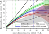Fig. 7 Sensitivity of the closed loop estimator for different numbers of controlled modes in the noise limited regime (coloured curves). The coloured areas emphasise the ±3 σ regions. The black dashed (resp. plain) line is the fitted (resp. theoretical) sensitivity of gcl ≃ 0.7 (resp. 1). The coloured dashed lines emphasise the lateral error at which the panels of Fig. 8 are displayed.

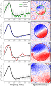Fig. 8 Sanity check of the fits introduced in Fig. 7 (arbitrary unit) for different numbers of controlled modes nmod and shift amplitudes |δth| ($\mathcal{A}$[δth] = 60°). Panels a, c, e, g: curves of the best temporal correlation fit ${\tilde{\mathcal{C}}}^{\mathrm{t}}$ (grey). Black curves: theoretical correlation curve ${\mathcal{C}}_0$ for δ → 0. Coloured curves: mean filter of ${\tilde{\mathcal{C}}}^{\mathrm{t}}$ with a sliding window of ±5 data points. Panels b, d, f, h: maps of the best fit correlation coefficients ${\tilde{\mathcal{C}}}^{2\mathrm{D}}$.

3.2.3 Bias induced by a frozen flow turbulence

In this section, turbulence is added to the system. Indeed, as mentioned by Heritier (2019, in Sect. 4.3) and discussed in Appendix C.2, the wind could bias the closed loop estimator when the temporal error is the dominant source of perturbation. To emulate the turbulence, a phase screen was generated for each simulation using the power spectrum density method proposed by McGlamery (1976) on a domain twelve times larger than the telescope pupil. To keep the phase screen 2D-periodic, no subharmonic was added (Lane et al. 1992). The screen was looped when translating the frozen flow according to the wind speed υ₀ and direction υ₀. All simulations were done for a typical Fried parameter of r₀ = 12 cm at λ₀ = 500 nm.

To assess the impact of a frozen flow turbulence on the closed loop estimator, both in terms of strength and orientation, simulations were run for wind speeds ranging from υ₀ = 1 m s⁻¹ to 80 m s⁻¹. The simulations being time-consuming, we used the symmetry of the problem to test wind directions only ranging from θ₀ = 0° to 90° every 7.5°. For each simulation, the system was initialised without any error δ = 0. n^mod = 500 modes are controlled. Batches of 500 consecutive closed loop iterations (0.5 s) are gathered to feed the closed loop estimator. In between each batch, the lateral error in the system was updated as follows: $${\mathit{\delta }}^{i+1}={\mathit{\delta }}^i+ธ\tilde{\mathit{\delta }}$$(42)

with the gain ธ = 0.5. Combined with the closed loop estimator sensitivity g^cl, Eq. (36), this leads to an approximated gain of 0.35 that insures a stable and slow convergence. The convergence values were obtained as described in Appendix F. Results are gathered in Fig. 9 for different photon noise regimes and for both the bias parallel (plain curves) and perpendicular (dashed curves) to the wind direction.

It first appears that as expected, the induced bias is along the wind direction (plain vs dashed curves). As seen by Heritier (2019, Sect. 4.3) with another mis-registration estimator, the bias amplitude depends on the ratio between the noise and the temporal error as well as the wind speed. For standard photon noise levels of n^ph between 10 and 100, it stays below 10% of a subaperture for wind speed below 37.5 m s⁻¹, that is to say below 20 mm. This should be compared to the total VLT pupil size of D = 8 m.

Close to the noiseless regime, with n^ph = 1000, the bias peaks a bit under 30% of a subaperture for low wind speeds. Some simulations, not shown here, indicate that this peak depends on the simulation resolution, suggesting an aliasing problem in the interpolation when translating the frozen screen. Better characterising this peak was not considered critical as such a situation would not be met in a real AO system. Indeed, errors which are not considered here would add up. Among others: the sensor readout noise and saturation, and some AO system non linearities such as the spot centroiding method or DM command clipping or saturation. And as discussed in Appendix C.2, the mis-registration estimator works better in a noise-limited regime. Considering only the photon noise is thus a conservative hypothesis.

Things worsen for wind speeds higher than υ₀ ≥ 37.5 m s⁻¹. For all the noise regimes, the estimator bias increases with the wind speed, until reaching a plateau around |δ| = 45%Δ. This saturation corresponds to the limit at which the AO loop becomes unstable when controlling 500 modes. This instability overcomes the wind perturbation in the loop global disturbance, stabilising the estimator. This result must be interpreted carefully. Indeed, for such high wind speeds, our end-to-end simulations reach their limits: during the exposure time, the wind evolution is not negligible and it should be averaged by simulating subframe steps.

As a consequence, the closed loop estimator was further tested on a more realistic turbulence, defined as the reference in the GPAO requirements (Le Bouquin 2023, Sect. 6). Table 3 gathers the parameters of its 5 layers. Its Fried parameter is r₀ = 10 cm. This corresponds to a seeing of 1″. This system is initialised with a lateral misalignment of |δ| = 70%Δ and $\mathcal{A}$[δ] = 35°, corrected every batches of 500 telemetry commands via Eq. (42) and still controlling n^mod = 500 modes.

The evolution of the lateral errors with the update iteration for different noise regimes is given in Fig. 10. For the first four iterations, the system is unstable and the convergence curves overlap for all noise regimes. They quickly drop around |δ| = 30%Δ. Despite a layer with a wind speed beyond 50 m s⁻¹, the divergence of the estimator remains under control. For the lowest noise level (red), it stays in the stability regime under |δ| = 35%Δ. For a realistic case of a noise dominated system (green), the corrective loop successfully tackles the initial lateral error and converges with a bias of |δ| ≃ 10% Δ.

We also emphasise here that real turbulence would be more complex than additive frozen flow layers. Any boiling or uncorrelated evolution would inject extra noise in the system producing the expected correlation curves, as explained in the first part of Appendix C.2. This would further participate to make the estimator robust to the frozen flow parts of the wind.

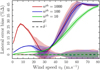Fig. 9 Influence of the wind speed υ0 and number of photons nph on the estimation of the lateral error δ = (δ‖, δ⊥) in the wind frame, parallel (plain curves) and perpendicular (dashed curves) to the wind direction θ0. The coloured areas emphasise the ±1 σ regions.

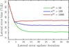Fig. 10 Convergence of the lateral error |δ| in function of the update iteration for the turbulence case of the GPAO requirements, see Table 3, and for different photon noise levels nph.

3.3 Experimental results: Auto-alignment in operation

In this section, the AO loop was closed using the parameters listed in Table 2. To test the closed loop estimator, we introduced a random lateral error to place the system at the limit of stability with the phase plate spinning at its maximal speed (υ₀ ≃ 8.4 m s⁻¹, r₀ ≃ 14 cm). This configuration leads to an unstable wave pattern on the DM commands (see Fig. 11c), which is seen by the WFS (see Figs. 11a,b) and that is typical to a lateral mis-registration (Heritier et al. 2018b). In addition, we kept the angle of 35° between the SH-WFS pupil and the DM grid. This angle can clearly be seen in the pattern orientation in between Figs. 11a,b and Fig. 11c.

We recall here that, depending on the context, the estimator can be used in two different ways: (1) to iteratively update the parameters of the command matrix of the system with a fixed lateral error until convergence or (2) to dynamically correct the system alignment until nominal registration is reached. The needs of GPAO introduced in Sect. 1 correspond to this latter option. As for the simulations of Sect. 3.2.3, the gain of the corrective secondary loop in charge of realigning the system is set to 0.5. Combined with the closed loop estimator sensitivity g^cl, Eq. (36), this leads to an approximated gain of 0.35.

As highlighted on Fig. 12, the corrective loop is run in two different situations. First, the phase plate is spinning. Then the corrective loop is opened and the phase plate is stopped to assess the bias induced by the wind on the closed loop estimator. Finally, a new set of corrective loop iterations is performed. In between all these steps, an IM is measured (with the phase plate stopped) to quantitatively retrieve the system misalignment with the AOF tool in SPARTA. The results are gathered in Table 4.

Despite starting in an unstable state, the corrective secondary loop efficiently converges in a few tens of iterations. At the start and stop of the phase plate, a small change in $\tilde{\mathit{\delta }}$ can be seen Fig. 12, suggesting that the frozen wind indeed induces a bias in the estimator. We further insist here that the values given in the figure are the lateral error computed by the closed loop estimator for each acquired telemetry batch of 500 frames. They consequently suffer from the underestimated sensitivity discussed in Sect. 3.2.2. For example, at the initial state, $\tilde{\mathit{\delta }}\simeq$ (8, 21)%Δ but SPARTA indicates that the real error is closer to $\tilde{\mathit{\delta }}\simeq$ (11, 45)%Δ, see Table 4.

With or without the phase plate, the convergence is stable but noisy with oscillations of a few percent. The IM measured after the corrective loop convergence with the phase plate spinning gives that |δ| ≃ 2.7%Δ. This bias is lower than the predictions of the simulations introduced in Sect. 3.2.3 suggesting that they were indeed conservative. Without the phase plate spinning, the lateral errors slightly drops to |δ| ≃ 2.5%Δ which is in the noise level of the estimator as shown in Fig. 12.

For information and sanity check, Figs. 11d,e give the correlation curve ${\tilde{\mathcal{C}}}^{\mathrm{t}}$ and map ${\tilde{\mathcal{C}}}^{2\mathrm{D}}$ for the point indicated with a star in Fig. 12. Looking at Fig. 11d, the main feature is a mismatch between the empirical correlation (grey/green) and the theoretical curve (black) at small frequencies. This discrepancy can be attributed to the wind, as discussed in Appendix C.2 and seen in frozen flow simulations.

Finally, the map of Fig. 11e shows that the command correlation leaves a strong trace in the 2D spatial frequency space with the typical ‘tip-tilt’ pattern. This pattern matches the theoretical area of the n^mod = 500 delimited by the coloured circle.

As a conclusion, these results prove that the closed loop estimator is able to correctly monitor and feed the corrective secondary loop. They also show that the theoretical model can successfully fit real data. In addition, in these tests, the wind induced by the phase plate had a negligible impact.

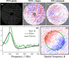Fig. 11 Example in the GPAO bench of the closed loop estimator. Panels a, b, c: SH-WFS pixel frame, WFS y-slopes and DM commands at the limit of stability before the alignment. Green circles: WFS pupil edges. Panel d: curves of the best temporal correlation fit ${\tilde{\mathcal{C}}}^{\mathrm{t}}$ (grey), of the mean filter of ${\tilde{\mathcal{C}}}^{\mathrm{t}}$ with a sliding window of ±5 data points (green), and of the theoretical correlation ${\mathcal{C}}_0$ (black). Panel e: map of the best fit correlation coefficients ${\tilde{\mathcal{C}}}^{2\mathrm{D}}$. The green circle encompasses the frequency space theoretically controlled by the command matrix.

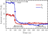Fig. 12 Convergence of the lateral error corrective loop with the closed loop estimator. Double arrows indicate when the phase plate and the corrective loop are active. The stars indicate the iteration at which Figs. 11d,e are displayed.

4 Conclusions and perspectives

In this work, we introduce two novel methods to estimate the lateral misalignment of an AO system. First, their underlying theory is presented. Then, we describe how their performance was tested in simulations. Finally, they were experimentally validated in the GPAO development bench with a system still largely under development and not yet fully characterised. These methods will be at the core of the GPAO system auto-alignment strategy while in operation to keep the AO performances at their optimal level throughout the observations. These methods were presented in the context of the GPAO system for its 40×40 SH-WFS mode. They were also successfully tested in the bench for the other GPAO configurations (30×30 and 9×9) and, as discussed below, they can be adapted to other AO systems, in particular for the future ELTs.

4.1 Perturbative modal estimator

This estimator uses the spatial 2D representation of the interaction matrix to look for spatial correlations of the measures with a reference. Not based on a complex model fitting, this method has the advantages to be fast and reliable, with a large capture range and a high S/N and is robust to loosely constrained higher-order mis-registrations such as clocking (to a few degrees) or stretch (to a few percent). An interesting by-product of the method is an estimation of the IM amplitude.

In this work, the reference is a synthetic IM, but an experimental reference measured during calibration could also be used, avoiding the need to rely on a possibly complex PSIM model of the system. A possible evolution of this method could be to totally get rid of the need of a reference IM. For example, by focussing on purely symmetric or anti-symmetric modes, looking at the symmetries of the modes in the measured IM and their auto-correlation should suffice to estimate the system decentering.

In this paper, we focus on a pertubative approach in open loop where the modal IM is actively measured by injecting modes in the system. We also tested that the method works in closed loop. The results are not presented in this paper but the lateral error is successfully retrieved. Naturally, the amplitude estimate is not reliable as the perturbations are fought by the AO loop.

In this work, we assume that the modal IMs are obtained with an invasive approach such as fast ‘push-pull’ of the modes (Kasper et al. 2004; Oberti et al. 2006; Kolb 2016) or via command modulation (Esposito et al. 2006; Pinna et al. 2012; Kolb 2016). The next step will be to test the estimator on the IM fully estimated from loop telemetry, for example as described by Béchet et al. (2012), based on the correlation between the slopes and the commands. Such IMs are generally noisy, but we have shown in this study that the estimator is robust to a high level of noise. Doing so would make the method non-pertubative, but potentially biased by the wind in case of a strong frozen flow, as discussed by Heritier (2019, in Sect. 4.3).

The method could also be extended to measure higher orders of mis-registration such as clocking or stretches. Nonetheless, these problems do not have a simple analytical solution as for the lateral errors, Eq. (7) and would surely imply iterative fitting of the parameters or extensive traversal of the parameter space.

In this work, we studied the influence of the number of KL modes in Appendix A, but we did not dig into optimising the subset of modes in order to maximise the estimator performances. We chose the pragmatic approach to select modes that will be seen and controlled by all the GPAO modes. Nonetheless, it is known that different modes do not provide the same sensitivity to the mis-registration parameters (Heritier et al. 2018b). We could optimise the modal shapes to improve the lateral resolution or the capture range and to avoid angular redundancy to prevent multiple secondary maxima in individual modal correlations or if looking for the clocking for example. Nevertheless, Heritier et al. (2021) have shown that fine tuning the modes is not critical.

Finally, this method was presented in the context of a SH-WFS, but it could be extended to other spatial WFS. For example, it could be used for the sub-pixel alignment of the pupil images of a pyramid WFS which also contain spatial information.

4.2 Non-perturbative closed loop estimator

This estimator uses the temporal correlation of the noise in the 2D representation of the DM commands in the closed loop telemetry to identify cross-talks between symmetric and anti-symmetric spatial frequencies. The main advantage of this method, and at the origin of its development, is its sparsity in the Fourier domain. Thus, this method is fast and particularly suited for systems with ever increasing numbers of actuators such as future ELTs, both in terms of execution time and memory requirements. GPAO will serve as an on-sky demonstrator of this technique, which is the current baseline to monitor and drive the quaternary DM for the ESO ELT in its engineering single conjugated AO mode, based on a pyramid WFS operating in the near infrared (Bonnet et al. 2023).

In addition, in the frequency domain, the impact of a frozen flow is also sparse, theoretically reducing the bias induced by the wind on the estimator. We nonetheless showed via simulations that for frozen flows with high wind speeds, the induced bias could diverge towards the loop stability limit. Nonetheless, the bias induced by the wind was not considered of high concern since the efficiency of the method interestingly increases with the noise in the system, as already intuited by Heritier (2019, Sect. 4.1.3). This makes it suitable to AO loops pushed at their limits (low magnitude or limit of stability or linearity) and for real systems always noisier than simulations. Nevertheless, a possible evolution of the method would be to further work on its de-biasing, for example by setting the weights of the correlation curve fitting to zero for low temporal frequency corresponding to the maximal awaited wind-induced signal. As seen in Fig. C.1b, this would depend on the spatial frequency insuring a correct number of data points through all the controlled space. Another solution would be to find a merit criterion on the correlation curves when solving Eq. (33). Indeed, the correlation signal induced by the wind strongly changes the shape of the theoretical correlation curves of the noise and should be quantifiable. Another direction to investigate is the exploitation of the real part of the correlation curves. It is discarded by the estimator of the proposed method, but the mixture of the noise propagation and the turbulence propagation should create a non-zero signal in the real part of the command correlation.

Another interesting features of the method is that it does not rely on a model of the AO system. Having access to the telemetry of a 2D spatial observable of the closed loop is sufficient. This could be the DM commands, as in this work, or directly the WFS measurements. This makes it particularly suitable to the pyramid WFS which directly gives the Hilbert transform of the incident wavefront perturbations in the telescope pupil for the non-modulated spatial frequencies. Nonetheless, these WFSs have a lower noise propagation than SH-WFSs, which could make them more sensitive to the wind bias, as noticed by Heritier (2019, Sect. 4.4). Therefore, further quantitative analyses should be performed before translating the results to such WFSs.

In addition, this method depends on only a limited number of parameters. We have seen that the shape of correlation signals are very sensitive to these parameters. They were fixed in this study, but a possible evolution would be to fit these parameters along with the lateral errors in a global inverse problem approach. On top of potentially reducing the estimator bias, this could also provide a supplementary way to monitor the loop gain or RTC performances.

A main drawback of this closed loop estimator is that it does not provide absolute measurements. It is relative to the registration state used to generate the command matrix. We showed that the measurement sensitivity is a priori unknown but nonetheless less than one. This guarantees a stable convergence in closed loop. The method is therefore suitable both for optical compensation by means of a pupil steering actuator (as for GPAO) or numerical compensation by command matrix updates derived from the accumulated error measurements, as for example described by Heritier et al. (2021).

Currently, this estimator was developed for lateral error monitoring which are ‘zero-order’ mis-registrations. This means that they only couple symmetric and anti-symmetric parts of the same spatial frequencies. A work is undergoing to extend this method to ‘first-order’ mis-registrations (clocking, magnification, and anamorphoses) with promising results. The difficult part is that such errors couple neighbouring spatial frequencies k and k + δk, increasing the complexity of the block diagram of Fig. 5 and the resulting correlation curves. Nonetheless, the estimators remain sparse in the Fourier domain and thus fast and scalable to complex systems.

In conclusion, a long-term perspective for both estimators would be their adaptation beyond single conjugated AO to multi-conjugated AO systems composed of multiple DMs and multiple WFSs. If the adaptation of the pertubative 2D modal estimator were to be straightforward, this would be less so the case for the non-perturbative closed loop estimator. Indeed, mis-registrations between the different subsystems will produce numerous cross-talks potentially difficult to disentangle in the observable temporal correlations.

Acknowledgements

This project has received funding from the European Union’s Horizon 2020 research and innovation programme under grant agreements No 101004719 and European Research Council (ERC)/CoG – 866070.

Appendix A Impact of the number modes on the 2D modal estimator

Even if optimising the shape and the number of modes used in the modal fit was beyond the scope of the paper, the impact of the number of selected KL modes is presented in Fig. A.1 for different noise configurations σ^slope on the IM slopes. For each case, 1000 random simulations were performed. To assess the noise propagation of the estimator, m^up was set to 100, leading to a theoretical resolution of one percent via the super-resolved map α. The lateral shift was fixed to δ_x = δ_y = δ₀ = 4.18Δ. Thus the problem is symmetric and the figure presents the global statistics of $\{{\tilde{\delta }}_x-{\delta }_0,{\tilde{\delta }}_y-{\delta }_0\}.$.

The figure shows that the IM noise level has a limited impact. Indeed, for m^KL,max ≥ 50, the bias and the standard deviation of the estimator lie within the chosen target of 1/8 = 12.5% of a subaperture for all the tested noise levels. The number of fitted modes appears as the key parameter of the method in order to limit the noise propagation and increase the achievable accuracy. This is expected since (1) increasing the number of modes allow us to average a larger number of noisy measurements, thus improving the S/N; (2) higher order modes show more high resolution features and thus gives access to a higher sensitivity. As a side remark, this figure also also supports the fact that any bias induced by the zero-padding strategy for the oversampling of the α-map is marginal (a few percent) in regard to the initial resolution (the subaperture pitch Δ).

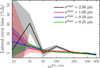Fig. A.1 Lateral error bias of the 2D correlation method in function of the noise σslope on the slopes of the IM and the number of fitted modes. The coloured areas emphasise the ±σ regions.

Appendix B Cross-talk with other mis-registrations

In this appendix, we introduce the impact of rotation and stretch misalignments on the performances of the proposed estimators. These two types of first order mis-registration are the most common ones with anamorphosis. This latter behaves as a stretch in our context and is consequently not presented.

Appendix B.1 Perturbative 2D modal estimator

The robustness of the 2D modal estimator in presence of other mis-registrations was assessed by simulating the convergence of a corrective loop on the lateral error. The initial lateral error was fixed to δ = (δ_y, δ_y) = (4.18, 3.73)Δ. We kept the parameters of Sect. 2.2: σ^slope = 0.25 pixel, m^{KL, max} = 50, m^up = 8. The corrective loop Eq. (42) is closed with a gain of ธ = 1.

Figures B.1 and B.2 present the evolution of |δ| with the iterations of the corrective loop for different mis-registration magnifications and angles respectively. The estimator is robust to extreme stretches, with a convergence within the resolution of the estimator 1/m^up achieved in two iterations. Similar results are obtained on the angle up to a mis-registration of 10°. Performances then quickly degrade above this threshold.

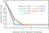Fig. B.1 Convergence of the lateral error after a few iterations of the corrective loop with the 2D modal estimator in function of the misregistration magnification ρ (square root scale).

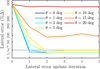Fig. B.2 Convergence of the lateral error after a few iterations of the corrective loop with the 2D modal estimator in function of the misregistration angle θ (square root scale).

Appendix B.2 Non-perturbative closed loop estimator

For the closed loop estimator, the context is different than with the 2D modal estimator: any mis-registration must be small enough to permit the AO loop closure. Otherwise, the loop diverges and this estimator does not apply since such a situation generally triggers the loop opening by the system. In this context, any small mis-registration on the angle, δ_θ, or the stretch, δ_ρ, is associated with the following transformation matrices: $$\left[\begin{array}{cc}1& +{\delta }_{\theta }\\ -{\delta }_{\theta }& 1\end{array}\right]\text{ and }\left[\begin{array}{cc}1+{\delta }_{\rho }& 0\\ 0& 1+{\delta }_{\rho }\end{array}\right]\text{. }$$(B.1)

Equation (B.1) shows that a lateral error in a given direction will slightly leak (1) towards its perpendicular counterpart in presence of a rotation error and (2) towards its neighbouring spatial frequency in the same direction in presence of a magnification error. This leakage should be negligible, most of the correlation signal staying within its own spatial frequency.

Similar as for the 2D modal estimator, the robustness of the closed loop estimator was assessed by simulating the convergence of a corrective loop on the lateral error. The initial lateral error was fixed to δ = (δ_x, δ_y) = (25,0)%Δ. As in Sect. 3.2.3, batches of 500 closed loop iterations controlling 500 modes are gathered to feed the estimator and the corrective loop Eq. (42) is closed with a gain of ธ = 0.5.

Figures B.3 and B.4 present the evolution of δ_x with the iterations of the corrective loop for different mis-registration magnifications and angles respectively. In all cases, the corrective loop successfully converges towards a null lateral error. When the loop is stable, for |θ| ≤ 1.5° and |ρ| ≤ 2%, the accuracy is below ±1%Δ. Above these thresholds, the closed loop is unstable. Its divergence is prevented by the clipping of the DM commands. In this situation, the accuracy nevertheless stays under control, within ±5%Δ.

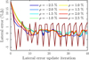Fig. B.3 Convergence of the lateral error after a few iterations of the corrective loop with the closed loop estimator in function of the misregistration magnification ρ (square root scale).

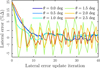Fig. B.4 Convergence of the lateral error after a few iterations of the corrective loop with the closed loop estimator in function of the misregistration angle θ (square root scale).

Appendix C Closed loop transfer functions

In this appendix, we derive the transfer functions introduced in Sect. 3.1.2. To ease the reading, we use the notation ‘$h(f)=\underset{\_}{h}$’⁸ to highlight the dependency in terms of f. As already discussed, we work under the assumptions of Eq. (14) that the transfer functions are identical for the two spatial modes. It is also implied that all this appendix is written for a given spatial frequency, k.

In doing so, the diagram of Fig. 5 is expressed as: $$\{\begin{array}{rl}{\underset{\_}{w}}_1=& -\cos \theta \left(\underset{\_}{A}\underset{\_}{C}(\underset{\_}{S}{\underset{\_}{w}}_1+{\underset{\_}{n}}_1)\right)+{\underset{\_}{p}}_1\\ & -\sin \theta \left(\underset{\_}{A}\underset{\_}{C}(\underset{\_}{S}{\underset{\_}{w}}_2+{\underset{\_}{n}}_2)\right),\\ {\underset{\_}{w}}_2=& -\cos \theta \left(\underset{\_}{A}\underset{\_}{C}({\underset{\_}{w}}_2+{\underset{\_}{n}}_2)\right)+{\underset{\_}{p}}_2\\ & +\sin \theta \left(\underset{\_}{A}\underset{\_}{C}(\underset{\_}{S}{\underset{\_}{w}}_1+{\underset{\_}{n}}_1)\right).\end{array}$$(C.1)

Introducing: $$\{\begin{array}{l}\underset{\_}{\mu }\triangleq \underset{\_}{A}\underset{\_}{C}\underset{\_}{S},\\ \underset{\_}{\mathrm{\Delta }}(\theta )\triangleq 1+2\underset{\_}{\mu }\cos \theta +{\underset{\_}{\mu }}^2,\end{array}$$(C.2)

Eq. (C.1) can be rewritten in a matrix shape: $$\mathit{M}(\theta )\left[\begin{array}{l}{\underset{\_}{w}}_1\\ {\underset{\_}{w}}_2\end{array}\right]=-\underset{\_}{A}\underset{\_}{C}\mathit{R}(\theta )\left[\begin{array}{l}{\underset{\_}{n}}_1\\ {\underset{\_}{n}}_2\end{array}\right]+\left[\begin{array}{l}{\underset{\_}{p}}_1\\ {\underset{\_}{p}}_2\end{array}\right],$$(C.3)

with: $$\{\begin{array}{l}\underset{\_}{\mathit{M}}(\theta )\triangleq \left[\begin{array}{cc}1+\underset{\_}{\mu }\cos \theta & +\underset{\_}{\mu }\sin \theta \\ -\underset{\_}{\mu }\sin \theta & 1+\underset{\_}{\mu }\cos \theta \end{array}\right],\\ \mathit{R}(\theta )\triangleq \left[\begin{array}{ll}+\cos \theta & +\sin \theta \\ -\sin \theta & +\cos \theta \end{array}\right].\end{array}$$(C.4)

Noticing that: $$\{\begin{array}{l}{\underset{\_}{\mathit{M}}}^{-1}(\theta )=\underset{\_}{\mathrm{\Delta }}(\theta {)}^{-1}\underset{\_}{\mathit{M}}(-\theta ),\\ \underset{\_}{\mathit{M}}(-\theta )\mathit{R}(\theta )=\left[\begin{array}{lc}\underset{\_}{\mu }+\cos \theta & +\sin \theta \\ -\sin \theta & \underset{\_}{\mu }+\cos \theta \end{array}\right],\end{array}$$(C.5)

it comes: $$\begin{array}{rl}\left[\begin{array}{l}{\underset{\_}{w}}_1\\ {\underset{\_}{w}}_2\end{array}\right]=& -\frac{\underset{\_}{A}\underset{\_}{C}}{\underset{\_}{\mathrm{\Delta }}(\theta )}\left[\begin{array}{cc}\underset{\_}{\mu }+\cos \theta & +\sin \theta \\ -\sin \theta & \underset{\_}{\mu }+\cos \theta \end{array}\right]\left[\begin{array}{l}{\underset{\_}{n}}_1\\ {\underset{\_}{n}}_2\end{array}\right]\\ & +\underset{\_}{\mathrm{\Delta }}(\theta {)}^{-1}\underset{\_}{\mathit{M}}(-\theta )\left[\begin{array}{l}{\underset{\_}{p}}_1\\ {\underset{\_}{p}}_2\end{array}\right],\end{array}$$(C.6)

and from ${\underset{\_}{m}}_i=\underset{\_}{S}{\underset{\_}{w}}_i+{\underset{\_}{n}}_i$ for i ∈ {1,2}, we finally get: $$\begin{array}{rl}\left[\begin{array}{l}{\underset{\_}{m}}_1\\ {\underset{\_}{m}}_2\end{array}\right]=& \left[\begin{array}{l}{\underset{\_}{n}}_1\\ {\underset{\_}{n}}_2\end{array}\right]-\frac{\underset{\_}{\mu }}{\underset{\_}{\mathrm{\Delta }}(\theta )}\left[\begin{array}{cc}\underset{\_}{\mu }+\cos \theta & +\sin \theta \\ -\sin \theta & \underset{\_}{\mu }+\cos \theta \end{array}\right]\left[\begin{array}{l}{\underset{\_}{n}}_1\\ {\underset{\_}{n}}_2\end{array}\right]\\ & +\frac{\underset{\_}{S}}{\underset{\_}{\mathrm{\Delta }}(\theta )}\left[\begin{array}{cc}1+\underset{\_}{\mu }\cos \theta & -\underset{\_}{\mu }\sin \theta \\ +\underset{\_}{\mu }\sin \theta & 1+\underset{\_}{\mu }\cos \theta \end{array}\right]\left[\begin{array}{l}{\underset{\_}{p}}_1\\ {\underset{\_}{p}}_2\end{array}\right].\end{array}$$(C.7)

As the perturbations ${\underset{\_}{p}}_i$ and noises ${\underset{\_}{n}}_j$ are independent, the crossproduct of two different terms is null: $$⟨{\underset{\_}{p}}_i{\overline{\underset{\_}{n}}}_j⟩=⟨{\underset{\_}{p}}_i⟩⟨{\overline{\underset{\_}{n}}}_j⟩=0.$$(C.8)

Similarly, the noise in the two parts of the diagram of Fig. 5 are independent and: $$⟨{\underset{\_}{n}}_1{\underset{\_}{\overline{n}}}_2⟩=0.$$(C.9)

As discussed below, only $⟨{\underset{\_}{p}}_1{\overline{\underset{\_}{p}}}_2⟩$ may be different from zero. Finally, one can assume that the pairs of noise terms $({\underset{\_}{n}}_1,{\underset{\_}{n}}_2)$ and $({\underset{\_}{p}}_1,{\underset{\_}{p}}_2)$ have identical properties, leading to: $$\{\begin{array}{l}⟨{\underset{\_}{n}}_1{\underset{\_}{\overline{n}}}_1⟩=⟨{\underset{\_}{n}}_2{\underset{\_}{\overline{n}}}_2⟩={\mathcal{V}}_{\underset{\_}{n}},\\ ⟨{\underset{\_}{p}}_1{\underset{\_}{\overline{p}}}_1⟩=⟨{\underset{\_}{p}}_2{\underset{\_}{\overline{p}}}_2⟩={\mathcal{V}}_{\underset{\_}{p}}.\end{array}$$(C.10)

It is now possible to compute the expected covariances $⟨{\underset{\_}{m}}_i{\overline{\underset{\_}{m}}}_j⟩$ for different regimes.

Appendix C.1 Noise propagation

In the noise-limited regime, the turbulence perturbation terms ${\underset{\_}{P}}_i$ are assumed to be negligible. It comes from Eqs. (C.7) and (C.10) that: $$\{\begin{array}{l}⟨{\underset{\_}{m}}_i{\overline{\underset{\_}{m}}}_i⟩=({\left|\frac{1+\underset{\_}{\mu }\cos \theta }{\underset{\_}{\mathrm{\Delta }}(\theta )}\right|}^2+{|\frac{\underset{\_}{\mu }}{\underset{\_}{\mathrm{\Delta }}(\theta )}\sin \theta |}^2){\mathcal{V}}_{\underset{\_}{n}},\\ ⟨{\underset{\_}{m}}_1{\overline{\underset{\_}{m}}}_2⟩=2i\mathcal{I}[\frac{1+\underset{\_}{\mu }\cos \theta }{|\underset{\_}{\mathrm{\Delta }}(\theta ){|}^2}\overline{\underset{\_}{\mu }}\sin \theta ]{\mathcal{V}}_{\underset{\_}{n}}.\end{array}$$(C.11)

Then, using Eqs. (14) and (23), the correlation between ${\underset{\_}{c}}_1$ and ${\underset{\_}{c}}_2$ is written as: $${\mathcal{C}}_{{\underset{\_}{c}}_1,{\underset{\_}{c}}_2}(\theta )={\mathcal{C}}_{{\underset{\_}{m}}_1,{\underset{\_}{m}}_2}(\theta )$$(C.12) $$=2i\sin \theta \frac{\mathcal{I}[(1+\underset{\_}{\mu }\cos \theta )\overline{\underset{\_}{\mu }}]}{|1+\underset{\_}{\mu }\cos \theta {|}^2+|\underset{\_}{\mu }\sin \theta {|}^2}.$$(C.13)

And finally, for a mis-registration parameter tending towards zero: $${\mathcal{C}}_{{\underset{\_}{c}}_1,{\underset{\_}{c}}_2}(\theta )/\theta \underset{\theta \to 0}{\sim }2i\mathcal{I}\left[\frac{\overline{\underset{\_}{\mu }}}{1+\overline{\underset{\_}{\mu }}}\right]=i{\mathcal{C}}_0(f).$$(C.14)

Appendix C.2 Turbulence propagation

In the situation where the system noise is dominated by the turbulence disturbance, ${\underset{\_}{n}}_i$ are assumed to be negligible. It comes from Eqs. (C.7) and (C.10): $$\{\begin{array}{ll}⟨{\underset{\_}{m}}_1{\overline{\underset{\_}{m}}}_1⟩=& {\left|\frac{\underset{\_}{S}}{\underset{\_}{\mathrm{\Delta }}\theta )}\right|}^2[(|1+\underset{\_}{\mu }\cos \theta {|}^2+|\underset{\_}{\mu }\sin \theta {|}^2)\mathcal{V}\underset{\_}{p}\\ & -2\mathcal{R}[(1+\underset{\_}{\mu }\cos \theta )\overline{\underset{\_}{\mu }}\sin \theta ⟨{\underset{\_}{p}}_1{\overline{\underset{\_}{p}}}_2⟩],\\ ⟨{\underset{\_}{m}}_2{\overline{\underset{\_}{m}}}_2⟩=& {\left|\frac{\underset{\_}{S}}{\underset{\_}{\mathrm{\Delta }}(\theta )}\right|}^2[(|1+\underset{\_}{\mu }\cos \theta {|}^2+|\underset{\_}{\mu }\sin \theta {|}^2){\mathcal{V}}_{\underset{\_}{p}}\\ & +2\mathcal{R}[(1+\underset{\_}{\overline{\mu }}\cos \theta )\underset{\_}{\mu }\sin \theta ⟨{\underset{\_}{p}}_1{\overline{\underset{\_}{p}}}_2⟩]]\\ ⟨{\underset{\_}{m}}_1{\underset{\_}{\overline{m}}}_2⟩=& {\left|\frac{\underset{\_}{S}}{\underset{\_}{\mathrm{\Delta }}(\theta )}\right|}^2[2i\mathcal{I}[(1+\underset{\_}{\mu }\cos \theta )\underset{\_}{\overline{\mu }}\sin \theta ]{\mathcal{Y}}_{\underset{\_}{p}}\\ & +{|1+\underset{\_}{\mu }\cos \theta |}^2⟨{\underset{\_}{p}}_1{\underset{\_}{\overline{p}}}_2⟩\\ & -|\underset{\_}{\mu }\sin \theta {|}^2⟨{\underset{\_}{p}}_2{\underset{\_}{\overline{p}}}_1⟩].\end{array}$$(C.15)

In the situation where the turbulence perturbations are independent, $⟨{\underset{\_}{p}}_1{\overline{\underset{\_}{p}}}_2⟩$ = 0, Eq. (C.15) leads to the same results than for the noise limited regime of the previous section: $$\{\begin{array}{l}{\mathcal{C}}_{{\underset{\_}{c}}_1,{\underset{\_}{c}}_2}(\theta )={\mathcal{C}}_{{\underset{\_}{m}}_1,{\underset{\_}{m}}_2}(\theta )=2i\sin \theta \frac{\mathcal{I}|(1+\underset{\_}{\mu }\cos \theta )\underset{\_}{\overline{\mu }}|}{|1+\underset{\_}{\mu }\cos \theta {|}^2+|\underset{\_}{\mu }\sin \theta {|}^2},\\ {\mathcal{C}}_{{\underset{\_}{c}}_1,{\underset{\_}{c}}_2}(\theta )/\theta \underset{\theta \to 0}{\sim }2i\mathcal{I}\left[\frac{\overline{\mu }}{1+\overline{\underset{\_}{\mu }}}\right]=i{\mathcal{C}}_0(f).\end{array}$$(C.16)

This result was expected since in these two situations, ${\underset{\_}{n}}_i$ and ${\underset{\_}{p}}_i$ play a similar role of pure independent noises injected in the system with just a normalisation by $\underset{\_}{S}$. This normalisation factor is cancelled out when estimating the correlation via Eq. (23).

Nonetheless, ${\underset{\_}{p}}_1$ and ${\underset{\_}{p}}_2$ are not always independent. This is the case for a pure frozen flow, the typical worst case offender of mis-registration estimators (Heritier et al. 2019; Heritier 2019, Sect. 4.3). Indeed, in such a situation, the wavefront is expressed as: $$\mathit{w}=w_0\cos (2\pi k^T\cdot (x-\mathit{v}t)-{\phi }_0)$$(C.17) $$=w_0\cos (2\pi f^{\parallel }t+{\phi }_0){\mathit{w}}_1+w_0\sin (2\pi f^{\parallel }t+{\phi }_0){\mathit{w}}_2,$$(C.18)

with φ₀ a constant phase delay and with f^‖ the temporal frequency of the wind projected parallel to the spatial frequency, k: $$f^{\parallel }={\mathit{k}}^T\cdot \mathit{v}\text{. }$$(C.19)

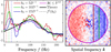Fig. C.1 Impact on the temporal correlation curves ${\tilde{\mathcal{C}}}^{\mathrm{t}}$ (left panel) and the map of the best fit correlation coefficients ${\tilde{\mathcal{C}}}^{2\mathrm{D}}$ (right panel) of a frozen flow perturbation of wind speed υ0 = 15 m s−1 aligned with a lateral error of δx = −20 %A in a noise limited regime nph = 10 and controlling nmod = 800. Coloured curves: best temporal correlation fit ${\tilde{\mathcal{C}}}^{\mathrm{t}}$ for different sets of controlled modes (mean filter with a sliding window of ±3 data points). Black curves: theoretical correlation curve ${\mathcal{C}}_0$. The coloured dashed lines emphasise the temporal frequencies f‖ = k0υ0 associated with the spatial frequencies k0 highlighted on the right panel.

Thus, $$\{\begin{array}{l}{p}_1(t)=w_0\cos (2\pi f^{\parallel }t+{\phi }_0),\\ p_2(t)=w_0\sin (2\pi f^{\parallel }t+{\phi }_0),\end{array}$$(C.20)

which, after a Fourier transform, gives in the frequency space: $$\{\begin{array}{l}{p}_1(f)=\frac{w_0}{2}({\mathrm{e}}^{i{\phi }_0}{\perp }_{f^{\parallel }}(f)+{\mathrm{e}}^{-i{\phi }_0}{\perp }_{-f^{\parallel }}(f)),\\ p_2(f)=\frac{w_0}{2i}({\mathrm{e}}^{i{\phi }_0}{\perp }_{f^{\parallel }}(f)-{\mathrm{e}}^{-i{\phi }_0}{\perp }_{-f^{\parallel }}(f)),\end{array}$$(C.21)

where ⊥_x is the Dirac function centered in x. Thus, we finally have: $$\{\begin{array}{ll}\mathbf{\forall }|f|\ne f^{\parallel },& ⟨p_1{\overline{p}}_2⟩(f)=0,\\ f=f^{\parallel },& {\mathcal{C}}_{c_1,c_2}\left(f^{\parallel }\right)\underset{\theta \to 0}{\sim }i,\\ f=-f^{\parallel },& {\mathcal{C}}_{c_1,c_2}(-f^{\parallel })\underset{\theta \to 0}{\sim }-i.\end{array}$$(C.22)

This means that a frozen flow turbulence has a minimal impact on the empirical correlation of Eq. (30). Only frequencies close to f ≃ k^T · υ should be impacted. In addition, these frequencies depend on the considered spatial mode k and consequently the impact on the estimator of Eq. (33) should be diluted among the controlled frequencies k ∈ $\mathcal{K}$^ctrl.

These different features are illustrated in Fig. C.1 for a noise limited regime n^ph = 10 and controlling n^mod = 800. The frozen turbulence flows at a speed of υ₀ = 15 m s⁻¹ in the same direction than a lateral error of δ_x = −20 %Δ. It seems that the wind has no qualitative impact on the best fit correlation map ${\tilde{\mathcal{C}}}^{2\mathrm{D}}$ (right panel of the figure). The purple temporal correlation curve ${\tilde{\mathcal{C}}}^{\mathrm{t}}$ is given by Eq. (39), while the other temporal correlation curves are obtained by replacing k ∈ $\mathcal{K}$^ctrl in the equation by: $$\{\mathit{k}\text{ s.t. }\mathit{k}\in {\mathcal{K}}^{\mathrm{c}\mathrm{t}\mathrm{r}\mathrm{l}}\text{ and }{k}_x=k_0\}\text{. }$$(C.23)

Different values of k₀ are displayed: 5D⁻¹ (red), 10D⁻¹ (green), 15D⁻¹ (blue). As expected, the frozen turbulence has only a limited impact on the empirical correlation which is centered around f^‖ = k₀υ₀. The rest of the curve still matches the theoretical asymptote of ${\mathcal{C}}_0$ well. The same conclusion applies to the global fit, in purple. Overall, only the low temporal frequencies are impacted.

Finally, the estimated lateral error is $\tilde{\mathit{\delta }}$ = (−11.5, 0) %Δ. This is in the same order of magnitude than the results of Fig. 7. This confirms that a wind blowing parallel to the lateral error should have a limited impact on the proposed closed loop estimator.

Appendix D Applying photon noise onto the SH-WFS slopes

In this appendix, we describe our method to add the photon noise directly onto the slopes of the geometrical model of the SH-WFS. For a given number of photon n^ph, the expected standard deviation of the wavefront phase on a subaperture is (Rousset 1999): $${\sigma }^{\mathrm{w}\mathrm{f}}=\frac{\pi }{\sqrt{2n^{\mathrm{p}\mathrm{h}}}}\frac{{\mathrm{\Theta }}^{\mathrm{s}\mathrm{p}\mathrm{o}\mathrm{t}}}{{\mathrm{\Theta }}^{\mathrm{d}\mathrm{i}\mathrm{f}}}\text{ (phase radian) },$$(D.1)

where Θ^spot and Θ^dif are the full widths at half maximum of the spot and the diffraction limited patterns of a subaperture. Noting d^sub the diameter of a subaperture, it becomes: $$\{\begin{array}{l}{\mathrm{\Theta }}^{\mathrm{s}\mathrm{p}\mathrm{o}\mathrm{t}}\simeq \frac{{\lambda }^{\mathrm{w}\mathrm{f}\mathrm{s}}}{r_0\left({\lambda }^{\mathrm{w}\mathrm{f}\mathrm{s}}\right)},\\ {\mathrm{\Theta }}^{\mathrm{d}\mathrm{i}\mathrm{f}}\simeq \frac{{\lambda }^{\mathrm{w}\mathrm{f}\mathrm{s}}}{d^{\text{sub }}},\end{array}$$(D.2)

where r₀(λ^wfs) is the Fried parameter scaled to the WFS wavelength. This leads to an optical path difference of: $${\sigma }^{\mathrm{O}\mathrm{P}\mathrm{D}}=\frac{{\lambda }^{\mathrm{w}\mathrm{f}\mathrm{s}}}{2}\frac{d^{\text{sub }}}{r_0({\lambda }^{\mathrm{w}\mathrm{f}\mathrm{s}}}\frac{1}{\sqrt{2n^{\mathrm{p}\mathrm{h}}}},$$(D.3)

and thus an angle across the subaperture diameter of: $${\sigma }^{\mathrm{p}\mathrm{h}}=\frac{{\lambda }^{\mathrm{w}\mathrm{f}\mathrm{s}}}{2r_0\left({\lambda }^{\mathrm{w}\mathrm{f}\mathrm{s}}\right)}\frac{1}{\sqrt{2n^{\mathrm{p}\mathrm{h}}}}\text{ (angle radian). }$$(D.4)

The different equivalent photon noises induced on the slopes by the number of photons are given in Table D.1.

Appendix E Impact of the telemetry batch size on the closed loop estimator

The influence of the telemetry batch size on the closed loop estimator was assessed in simulation by introducing a fixed lateral error of δ = (δ_x, δ_y) = (10,0) %Δ. For each tested batch size, 100 batches in a pure noise regime were gathered, controlling 500 modes.

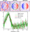Fig. E.1 Impact of the telemetry batch size on the map of the best fit correlation coefficients ${\tilde{\mathcal{C}}}^{2\mathrm{D}}$ (top panels) and the temporal correlation curves ${\tilde{\mathcal{C}}}^{\mathrm{t}}$ (bottom panel). The coloured circles emphasise the controlled frequency space.

Their statistics are shown in Table E.1. First, the sensitivity of g^cl ≃ 0.7 of the estimator can be seen with $({\tilde{\delta }}_x,{\tilde{\delta }}_y)$ ≃ (6.9,0.0) %Δ, in agreement with Fig. 7. Then, as expected, the noise on the estimated value decrease with the number of frames in the batch and is consistent on the x and y-axes. The size of 500 frames, used in this work, gives a standard deviation of ±0.25 %Δ. This was considered to be a good compromise between speed and accuracy, allowing for the corrective loop on the lateral error to be estimated and updated once every second.

For information, Fig. E.1 presents an example of the correlation patterns obtained when varying the size of the telemetry batch. The increase of the signal over noise ratio and the frequency resolution with the number of frames can clearly be seen in the correlation maps ${\tilde{\mathcal{C}}}^{2\mathrm{D}}$ (top panels) and temporal correlation curves ${\tilde{\mathcal{C}}}^{\mathrm{t}}$ (bottom panel).

Appendix F Estimating the lateral bias induced by the wind

In this appendix, we detail how the convergence values of the bias induced by the frozen flow wind are obtained from the iterative updates of the lateral errors with time. For n^ph = 10 and 100, n^it = 40 updates (spanning over 20 s) of δ were performed. For n^ph = 1000, the convergence is slower and n^it = 60 updates (spanning over 30 s) of δ were performed.

Figure F.1 shows the evolution of δ with the update iterations for different level of photon noise. Convergence is achieved despite being noisy. To robustly estimate the convergence value, an exponential law (dotted curves in the figure) is fitted in the data points of each direction parallel ‖ and perpendicular ⊥ to the wind’s direction: $${\delta }_{\parallel ,\perp }^i\simeq {\mathit{\vartheta }}_{\parallel ,\perp }(1-{\mathrm{e}}^{-{\mathit{ร}}_{\parallel ,\perp }(i-i_{\parallel ,\perp }^0)}).$$(F.1)

The fit of (ง, ร, i⁰) is performed by minimising the root mean square difference between the model and the simulation with the simplex search method of Lagarias et al. (1998), enforcing that 1/ร < 25. ง gives the convergence value and the bias induced by the wind on the closed loop estimator.

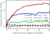Fig. F.1 Convergence of the lateral error δ in percent of subaperture pitch Δ in function of the update iteration for υ0 = 20 m s−1, θ0 = 30°, and for different photon noise levels nph (colours). Plain (resp. dashed) curves: lateral error δ‖ parallel (resp. δ⊥ perpendicular) to the wind direction. Dotted curves: fitted exponential law.

References

All Tables

All Figures

Fig. 1 General idea of the spatial 2D correlation method for different KL modes mKL ∈ {6, 20, 35, 46}. When different modes are applied on the DM (first line), the patterns seen by the WFS show different spatial scales (second line). The grey pixels correspond to the missing slopes wWFS (x) = 0 in the PSIM model that are hidden by the pupil. A lateral mis-registration would shift the peak in the correlation between the PSIM and the measured IM (third line).

In the text

Fig. 2 Simulated example of the spatial 2D correlation method. Panel a: simulation of a measured and shifted modal IM (x-slopes) for mKL = 35. The grey and dark pixels correspond to the non-valid slopes wvalid(x) = 0 in the measured IM. Panel b: cross-correlation of the shifted mode of Panel a with the reference modal IM for mKL = 35 (see Fig. 1). Panel c: map of the fitted coefficients α. Panel d: over-sampling of panel c with an interpolation via sinc functions.

In the text

	Fig. 3 Example in the GPAO bench of the 2D modal estimator. Panels a, b: SH-WFS pixels before and after the alignment. Green circles: WFS pupil edges. Panels c, e, f: x-slopes of the modal IM for mKL = 40 before (panel c) and after (panel e) alignment and reference (panel f). panel d: over-sampled map of the coefficient α before alignment.
In the text

	Fig. 4 Convergence of the lateral error corrective loop with the 2D modal estimator at GPAO preset.
In the text

	Fig. 5 Block diagram of the temporal coupling (in red) of the symmetric (cosine, in blue) and anti-symmetric (sine, in green) parts of a given spatial frequency k = (2/3D, 0) through the AO loop.
In the text

	Fig. 6 Imaginary part of the correlation curves ${\mathcal{C}}_{c_1,c_2}$ (θ, f) in a noise limited regime for various values of θ from 0° (blue) to 45° (red), every 5°. AO parameters: τWFS = 1 ms, g∫ = 0.5, gε = 0.
In the text

	Fig. 7 Sensitivity of the closed loop estimator for different numbers of controlled modes in the noise limited regime (coloured curves). The coloured areas emphasise the ±3 σ regions. The black dashed (resp. plain) line is the fitted (resp. theoretical) sensitivity of gcl ≃ 0.7 (resp. 1). The coloured dashed lines emphasise the lateral error at which the panels of Fig. 8 are displayed.
In the text

Fig. 8 Sanity check of the fits introduced in Fig. 7 (arbitrary unit) for different numbers of controlled modes nmod and shift amplitudes |δth| ($\mathcal{A}$[δth] = 60°). Panels a, c, e, g: curves of the best temporal correlation fit ${\tilde{\mathcal{C}}}^{\mathrm{t}}$ (grey). Black curves: theoretical correlation curve ${\mathcal{C}}_0$ for δ → 0. Coloured curves: mean filter of ${\tilde{\mathcal{C}}}^{\mathrm{t}}$ with a sliding window of ±5 data points. Panels b, d, f, h: maps of the best fit correlation coefficients ${\tilde{\mathcal{C}}}^{2\mathrm{D}}$.

In the text

References

- Åström, K., & Murray, R. 2021, Feedback Systems: An Introduction for Scientists and Engineers, 2nd edn. (Princeton University Press) [Google Scholar]
- Béchet, C., Tallon, M., & Thiébaut, É. 2012, in Adaptive Optics Systems III, 8447, eds. B. L. Ellerbroek, E. Marchetti, & J.-P. Véran, International Society for Optics and Photonics (SPIE), 84472C [Google Scholar]
- Bertrou-Cantou, A., Gendron, E., Rousset, G., et al. 2022, A&A, 658, A49 [NASA ADS] [CrossRef] [EDP Sciences] [Google Scholar]
- Beuzit, J.-L., Vigan, A., Mouillet, D., et al. 2019, A&A, 631, A155 [NASA ADS] [CrossRef] [EDP Sciences] [Google Scholar]
- Bonnet, H., Spyromilio, J., Rubin, A., & Esselborn, M. 2023, in Current designs of ELT AO system, AO4ELT7 [Google Scholar]
- Boyer, C. 2018, in Adaptive Optics Systems VI, eds. D. Schmidt, L. Schreiber, & L. M. Close (SPIE) [Google Scholar]
- Brusa, G., Riccardi, A., Wildi, F. P., et al. 2003, SPIE Conf. Ser., 5169, 26 [Google Scholar]
- Dai, G.-m. 1995, J. Opt. Soc. Am. A, 12, 2182 [NASA ADS] [CrossRef] [Google Scholar]
- Dembet, R. 2023, ESO, in RTC4AO Workshop [Google Scholar]
- Esposito, S., Tubbs, R., Puglisi, A., et al. 2006, SPIE Conf. Ser., 6272, 62721C [NASA ADS] [Google Scholar]
- Fried, D. L. 1977, J. Opt. Soc. Am., 67, 370 [NASA ADS] [CrossRef] [Google Scholar]
- Gendron, E., & Lena, P. 1994, A&A, 291, 337 [Google Scholar]
- Gilmozzi, R., & Spyromilio, J. 2007, The Messenger, 127, 11 [Google Scholar]
- GRAVITY Collaboration (Abuter, R., et al.) 2017, A&A, 602, A94 [NASA ADS] [CrossRef] [EDP Sciences] [Google Scholar]
- GRAVITY+ Collaboration (Abuter, R., et al.) 2022, The Messenger, 189, 17 [NASA ADS] [Google Scholar]
- Heritier, C. T. 2019, Ph. D. Thesis, Aix Marseille Université, France [Google Scholar]
- Heritier, C. T., Esposito, S., Fusco, T., et al. 2018a, MNRAS, 481, 2829 [Google Scholar]
- Heritier, C. T., Esposito, S., Fusco, T., et al. 2018b, SPIE Conf. Ser., 10703, 107034P [NASA ADS] [Google Scholar]
- Heritier, C. T., Neichel, B., Correia, C., et al. 2019, Video Mem. Soc. Astron. Ital., 1, 12 [Google Scholar]
- Heritier, C. T., Fusco, T., Oberti, S., et al. 2021, MNRAS, 504, 4274 [NASA ADS] [CrossRef] [Google Scholar]
- Johns, M. 2006, SPIE Conf. Ser., 6267, 626729 [NASA ADS] [Google Scholar]
- Kasper, M., Fedrigo, E., Looze, D. P., et al. 2004, J. Opt. Soc. Am. A, 21, 1004 [NASA ADS] [CrossRef] [Google Scholar]
- Kolb, J. 2016, SPIE Conf. Ser., 9909, 99090K [NASA ADS] [Google Scholar]
- Kolb, J., Madec, P. Y., Le Louarn, M., Muller, N., & Béchet, C. 2012, SPIE Conf. Ser., 8447, 84472D [NASA ADS] [Google Scholar]
- Lagarias, J. C., Reeds, J. A., Wright, M. H., & Wright, P. E. 1998, SIAM J. Optim., 9, 112 [CrossRef] [Google Scholar]
- Lai, O., Chun, M., Dungee, R., Lu, J., & Carbillet, M. 2021, MNRAS, 501, 3443 [NASA ADS] [CrossRef] [Google Scholar]
- Lane, R., Glindemann, A., & Dainty, J. 1992, Waves Random Media, 2, 209 [NASA ADS] [CrossRef] [Google Scholar]
- Le Bouquin, J.-B. 2023, ESO Technical Report, VLT-TRE-GRP-0031 [Google Scholar]
- Madec, P.-Y. 1999, Control Techniques (Cambridge University Press), 131 [Google Scholar]
- McGlamery, B. L. 1976, in Image Processing, ed. J. C. Urbach, 0074, International Society for Optics and Photonics (SPIE), 225 [NASA ADS] [CrossRef] [Google Scholar]
- Millour, F., Bério, P., Lagarde, S., et al. 2022, SPIE Conf. Ser., 12183, 121831X [NASA ADS] [Google Scholar]
- Moore, E. H. 1920, Bull. Am. Math. Soc., 26, 394 [Google Scholar]
- Neichel, B., Parisot, A., Petit, C., Fusco, T., & Rigaut, F. 2012, SPIE Conf. Ser., 8447, 84475N [NASA ADS] [Google Scholar]
- Oberti, S., Bonnet, H., Fedrigo, E., et al. 2004, SPIE Conf. Ser., 5490, 139 [Google Scholar]
- Oberti, S., Quirós-Pacheco, F., Esposito, S., et al. 2006, SPIE Conf. Ser., 6272, 627220 [Google Scholar]
- Oberti, S., Kolb, J., Le Louarn, M., et al. 2016, SPIE Conf. Ser., 9909, 99091U [Google Scholar]
- Oberti, S., Kolb, J., Madec, P.-Y., et al. 2018, SPIE Conf. Ser., 10703, 107031G [NASA ADS] [Google Scholar]
- Penrose, R. 1955, Math. Proc. Camb. Philos. Soc., 51, 406 [NASA ADS] [CrossRef] [Google Scholar]
- Pinna, E., Quirós-Pacheco, F., Riccardi, A., et al. 2012, SPIE Conf. Ser., 8447, 84472B [NASA ADS] [Google Scholar]
- Riccardi, A., Brusa, G., Salinari, P., et al. 2003, SPIE Conf. Ser., 4839, 721 [NASA ADS] [Google Scholar]
- Roddier, F. 1999, Adaptive Optics in Astronomy (Cambridge University Press) [CrossRef] [Google Scholar]
- Rousset, G. 1999, Wave-front Sensors (Cambridge University Press), 91 [Google Scholar]
- Shack, R. V., & Platt, B. C. 1971, in Spring Meeting of the Optical Society of America, 61, ed. F. D. Smith, 656 [Google Scholar]
- Shchekaturov, P. 2023, in RTC4AO Workshop [Google Scholar]
- Ströbele, S., Arsenault, R., Bacon, R., et al. 2006, SPIE Conf. Ser., 6272, 62720B [Google Scholar]
- Suárez Valles, M., Fedrigo, E., Donaldson, R. H., et al. 2012, SPIE Conf. Ser., 8447, 84472Q [Google Scholar]
For example the Fried geometry (Fried 1977), where the DM actuators are optically placed at the corner of the SH-WFS subapertures.
We notice that this constraint on the speed could be relaxed for the VLTI where the physics of the mis-registrations is bound to be slow after the preset. Nonetheless, we aim to test on-sky the method efficiency in preparation of the future ELTs where the timescale of the misalignment evolution will be much shorter.
In each instance of GPAO, the DM, placed in the Coudé train of its UT, is tilted with respect to the incident beam by an angle of ~ 13.3°, leading to a stretch of ~ 2.7% (Le Bouquin 2023) and ΔDM ≠ Δ.
As a side remark, the eight white squares in Fig. 3b come from the activation during the instrument calibration of the dark follower of the eight octants of the camera.
We notice here the possibility that g∫ and gε could be functions applied on ci and cδ and not pure scalars, especially if modal filtering is applied for control and leakage (Gendron & Lena 1994).
![$\[\underline{h}\]$](/articles/aa/full_html/2024/07/aa49311-24/aa49311-24-eq149.png)
All Tables
Statistics of the estimated lateral error in function of the telemetry batch size.