| Issue |
A&A
Volume 644, December 2020
|
|
|---|---|---|
| Article Number | A6 | |
| Number of page(s) | 8 | |
| Section | Astronomical instrumentation | |
| DOI | https://doi.org/10.1051/0004-6361/202037836 | |
| Published online | 24 November 2020 | |
Pyramid wavefront sensor optical gains compensation using a convolutional model
1
Aix Marseille Univ, CNRS, CNES, LAM, Marseille, France
e-mail: This email address is being protected from spambots. You need JavaScript enabled to view it.
2
ONERA The French Aerospace Laboratory, 92322 Châtillon, France
3
IFREMER, Laboratoire Detection, Capteurs et Mesures (LDCM), Centre Bretagne, ZI de la Pointe du Diable, CS 10070, 29280 Plouzane, France
4
W. M. Keck Observatory, 65 – 1120 Mamalahoa Hwy., Kamuela, HI 96743, USA
5
UK Astronomy Technology Centre, Blackford Hill, Edinburgh EH9 3HJ, UK
Received:
27
February
2020
Accepted:
26
May
2020
Abstract
Context. Extremely large telescopes are overwhelmingly equipped with pyramid wavefront sensors (PyWFS) over the more widely used Shack–Hartmann wavefront sensor to perform their single-conjugate adaptive optics (SCAO) mode. The PyWFS, a sensor based on Fourier filtering, has proven to be highly successful in many astronomy applications. However, this sensor exhibits non-linear behaviours that lead to a reduction of the sensitivity of the instrument when working with non-zero residual wavefronts. This so-called optical gains (OG) effect, degrades the closed-loop performance of SCAO systems and prevents accurate correction of non-common path aberrations (NCPA).
Aims. In this paper, we aim to compute the OG using a fast and agile strategy to control PyWFS measurements in adaptive optics closed-loop systems.
Methods. Using a novel theoretical description of PyWFS, which is based on a convolutional model, we are able to analytically predict the behaviour of the PyWFS in closed-loop operation. This model enables us to explore the impact of residual wavefront errors on particular aspects such as sensitivity and associated OG. The proposed method relies on the knowledge of the residual wavefront statistics and enables automatic estimation of the current OG. End-to-end numerical simulations are used to validate our predictions and test the relevance of our approach.
Results. We demonstrate, using on non-invasive strategy, that our method provides an accurate estimation of the OG. The model itself only requires adaptive optics telemetry data to derive statistical information on atmospheric turbulence. Furthermore, we show that by only using an estimation of the current Fried parameter r0 and the basic system-level characteristics, OGs can be estimated with an accuracy of less than 10%. Finally, we highlight the importance of OG estimation in the case of NCPA compensation. The proposed method is applied to the PyWFS. However, it remains valid for any wavefront sensor based on Fourier filtering subject from OG variations.
Key words: instrumentation: adaptive optics / atmospheric effects
© V. Chambouleyron et al. 2020
 Open Access article, published by EDP Sciences, under the terms of the Creative Commons Attribution License (https://creativecommons.org/licenses/by/4.0), which permits unrestricted use, distribution, and reproduction in any medium, provided the original work is properly cited.
1. Introduction
The pyramid wavefront sensor (PyWFS) is an optical device used to perform wavefront sensing, which was first proposed in 1996 (Ragazzoni 1996). Inspired by the Foucault knife test, the PyWFS is a pupil plane wavefront sensor (WFS) performing optical Fourier filtering thanks to a glass pyramid located in the focal plane (see Fig. 1). This pyramid splits the electromagnetic (EM) field into four beams, each producing four different filtered images of the entrance pupil. This filtering operation converts phase information at the entrance pupil into amplitude information at a pupil plane where a quadratic sensor is used to record the signal. The PyWFS usually includes an additional optical device called a modulation mirror. This mirror moves the point spread function (PSF) around the apex of the pyramid, which allows for an increase in the linearity range of the device at the expense of sensitivity.
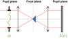 |
Fig. 1. Diagram of PyWFS, Fourier filtering WFS. A pyramidal mask is placed at a focal plane to achieve optical filtering. The output signal I(ϕ) shows a relationship to the entrance phase ϕ. |
The PyWFS displays higher sensitivity than the Shack–Hartmann wavefront sensor (SHWFS) and is therefore a key element for present and future adaptive optics (AO) systems. As an example, this device will be used to perform the single-conjugate adaptive optics (SCAO) mode of all European extremely large telescope (ELT) first light instruments (Neichel et al. 2016; Davies et al. 2018; Hippler et al. 2019). Unfortunately, the PyWFS exhibits non-linear behaviours and the relationship between the produced signal and the incoming wavefront is not as straightforward as with the SHWFS. The complexity and the limited knowledge on the nature of the PyWFS measurements has led to extensive studies of this device (Vérinaud 2004; Guyon 2005; Korkiakoski et al. 2007; Hutterer et al. 2019) in order to analytically describe its linear response. However, it is possible to describe the PyWFS as a convolutional system that can be fully characterised by the knowledge of its impulse response, as is widely done for many physical systems. The advantages of such a convolutional description are numerous: it allows for a fast numerical computation of the response of a sensor to a given input phase and gives the frequency-dependent sensitivity through the transfer function of the system. A first step in that direction was proposed by Hutterer et al. (2019), but the model suffers from strong approximations; for example, the PyWFS is described as two rooftop masks and some terms are neglected to simplify calculations. To the best of our knowledge, the most complete study to date of the PyWFS as a convolutional system has been proposed by Fauvarque et al. (2019). In this model, the PyWFS is simply described by its three main properties: the shape of the pyramid mask m, the modulation function w, and the entrance pupil geometry 𝕀p (see Fig. 2). According to this description, the impulse response of the system is given by the following equation:
 (1)
(1)
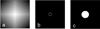 |
Fig. 2. Panel a: shape of the pyramid mask – arg(m). Panel b: modulation function – w. Panel c: pupil shape – 𝕀p. |
where Im is the imaginary part,  the Fourier transform operator, and ⋆ the convolution symbol.
Now that the PyWFS has captured the interest of AO scientists, one of its major limitations needs to be handled, namely its strong non-linear behaviour which leads to a spatial frequency-dependent loss of sensitivity during on-sky operations. This loss of sensitivity can be captured in a quantity called optical gains (OG) (Korkiakoski et al. 2008; Deo et al. 2019a). Tracking the OG during on-sky operations has therefore become one of the key priorities to fully control PyWFS measurements.
Optical gains originating from non-linear behaviours have already been recognised in other WFSs, such as the quad-cells SHWFS (Véran & Herriot 2000) or the Zernike WFS (Vigan et al. 2019). The main impact of OG in closed-loop operation is to introduce an error in the wavefront reconstruction. This error becomes predominant in the case of bad seeing conditions or when pointing at extended objects. There are new robust strategies available for on-the-fly optimisation of the loop gains to mitigate the reconstruction error impacted by OGs (Deo et al. 2019b). However, these techniques do not give direct access to the actual OG values (see Sect. 4). In fact, knowledge of OG is essential for non-common path aberrations (NCPA) correction, which is emerging as a critical step in wavefront control for systems based on PyWFS (Esposito et al. 2015). Knowledge of OG is also a key issue in PSF reconstruction, where accurate analysis of loop telemetry data is paramount. The objective of this paper is to present a new strategy based on a physical description of the PyWFS to quickly and accurately compute the OGs independently from temporal loop gains.
In Sect. 2, we present the definition of the OG and ways to better understand the physical nature of OG, which are generated by residual phases on the PyWFS. In Sect. 3, we show that it is possible to use the convolutional model to accurately compute OG, provided there is some statistical information on the shape of the residual phases. Finally, in the last section of this paper, we demonstrate the superiority of our method for NCPA compensation.
2. Definition of optical gains and application to PyWFS in presence of residual phases
2.1. Interaction matrix as a linear model of the PyWFS
The WFS can be described by a matrix that fully encodes the linear behaviour of the system. This so-called interaction matrix (IM) is computed through a calibration process by recording the slopes of the linear responses of the WFS to a set of incoming phases ϕi. Combined, these wavefronts represent the basis of the phase space we want to control. For each mode, the slopes of the linear response δIcalib(ϕi) (Fig. 3) can be computed through the following operation, often referred to as “push-pull”:
 (2)
(2)
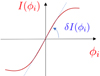 |
Fig. 3. Sketch of the PyWFS response curve for a given mode ϕi. The push-pull method around a null-phase consists in computing the slope of this curve for a = 0. |
where Icalib is the recorded intensity on the WFS detector. A reference signal, corresponding to a flat wavefront in the pupil plane, is also subtracted from this value. In this paper, we use the full-frame definition for the PyWFS signal, however this work can easily and straightforwardly be applied to the slope-like definition of the PyWFS measurements. In the previous equation, a represents the amplitude of the mode used for calibration. The quantity a should be as small as possible in order to stay within the linear regime of the sensor. But in reality, we want it to be large enough to ensure a satisfactory signal-to-noise ratio, while at the same time staying within the linearity regime. This maximisation of signal-to-noise ratio during calibration can be helped by using optimal calibration strategies, such as the Hadamard approach (Meimon et al. 2015). The IM computed during the calibration process IMcalib is then the concatenation the slopes recorded for all modes, that is
 (3)
(3)
In the well-known inverse problems framework, this calibration step is actually a way to compute the linear forward operator of our system, associating the incoming wavefront with pyramid measurements.
2.2. Optical gains: An offset between calibration regime and on-sky regime
The IMcalib is computed in a specific regime that we call the calibration regime. The calibration is usually done using a point-like source around a flat wavefront (no reference phase) and for a given modulation radius.
During operation, which we call the on-sky regime, the WFS differs inevitably from the calibration regime, if nothing else because we cannot reach the perfect diffraction limit of the telescope. Because of the non-linear nature of the PyWFS, this leads to a change in the behaviour of the sensor. It is possible to account for these non-linearities by considering the PyWFS as a sensor with a varying linear behaviour that depends on the current sensing regime. We therefore hypothesise that the behaviour of the sensor in the on-sky regime can be described by an IM that we call IMonSky. In that case, the linear behaviour has to be measured again for an accurate description of the direct problem, that is
 (4)
(4)
When the PyWFS is working around a non-null reference phase, we have the following relationship:
 (5)
(5)
because of the non-linear behaviour of the PyWFS, we have Icalib(aϕi + ϕres) ≠ Icalib(aϕi)+Icalib(ϕres) and therefore
 (6)
(6)
which naturally leads to offsets between IMcalib and IMonSky.
We define the optical transfer matrix Topt as the transfer matrix describing the offsets between the on-sky regime and the calibration regime. This matrix is a square matrix of size Nmodes × Nmodes, where
 (7)
(7)
To obtain the correct linear description of the sensor in a given sensing regime, we therefore need to adjust the IM computed during calibration by the optical transfer matrix.
From the equation above, we can write the exact definition of the optical transfer matrix as follows:
 (8)
(8)
2.3. Diagonal approximation and OG definition in the PyWFS measurement space
The diagonal approximation can strongly simplify the computation of Topt. This approximation consists in assuming that Topt is a diagonal matrix (Deo et al. 2019a), meaning there is no cross-talk between modes when we are switching from the calibration regime to the on-sky (or sensing) regime. In other words, the slope of the linear behaviour for each mode ϕi is increased or reduced by a scalar factor G(ϕi) called the modal OG.
In the case of the diagonal approximation, we can define the modal OG G(ϕi) without having to use the pseudo-inverse  (which depends on the condition number): we propose the use of the scalar product ⟨⋅|⋅⟩ defined in the measurement space to compare δIonSky(ϕi) and δIcalib(ϕi) for each mode ϕi as follows:
 (9)
(9)
The expression ⟨δIonSky(ϕi)|δIcalib(ϕi)⟩ represents the projection of the measurement in the sensing regime onto the measurement in the calibration regime and ⟨δIcalib(ϕi)|δIcalib(ϕi)⟩ is a normalisation term. The definition of OG given in this work differs slightly from those previously given in the literature (Korkiakoski et al. 2008; Deo et al. 2019a), and has the advantage of being independent of the reconstructor. This is a description in measurement space only. An equivalent formulation of Eq. (9) in terms of matrices is the following:
 (10)
(10)
where Gopt is a vector containing all the G(ϕi) for i ∈ [1, Nmodes].
2.4. Impact of residual phases on the PyWFS impulse response
The offset experienced by IMcalib changes at each measurement because ϕres is a time-varying quantity. That is to say that IMonSky is changing at every iteration, depending on the content of ϕres. Although it seems hard to determine the state of IMonSky at each instant, we can find a way to compute the averaged state of the sensing regime ⟨IMonSky⟩t, which gathers ⟨δIonSky(ϕi)⟩t for each mode. This averaged state is written as
 (11)
(11)
In this regard, we rely on the convolutional formalism of the PyWFS proposed by Fauvarque et al. (2019). Within the framework of this model, it is possible to compute an analytic function to take into account the impact of residual phases on PyWFS measurements. The sensing regime is then described by a PyWFS for which the modulation function (see Eq. (1)) is changed according to this formula:
 (12)
(12)
where Dϕres is the residual phase structure function. This equation provides a fundamental insight into PyWFS measurements in the presence of residual phases. It was well-known that residual phases act as an extra modulation that lowers the sensitivity of the pyramid. We are now able to quantify this loss: the impact depends on residual phases statistics through the structure function, and therefore through the power spectral density (PSD). It is then possible to define its new impulse response in the averaged sensing regime assuming isotropy and stationarity of the residual phases as follows:
 (13)
(13)
We note that the modulation function is the only quantity affected here. This means that the impact of residual phases can be described as a collection of incoherent tip-tilt offsets during one measurement cycle. Changing from an apparently coherent offset to an incoherent offset comes from the time averaging operation. This is very well understood in the image formation field through the derivation of the atmospheric transfer function Roddier (1981). By averaging over time, we can derive an analytic formulation for the long-exposure seeing limited PSF, which cannot be fully described using a coherent phase aberration in the pupil plane.
In this section, we presented a new measurement space based definition for the OG. We also explained how they naturally emerge from PyWFS non-linearities when working with offsets between calibration and sensing regimes. In the following part, we propose a new method based on the convolutional model to perform a fast and accurate computation of the OG.
3. New strategy to compute PyWFS modal optical gains through the convolutive model
3.1. Convolutional formalism: A path to optical gains computation
In case of OG introduced by residual phase, the diagonal approximation ensures that the knowledge of the diagonal elements of Gopt is sufficient to compute IMonSky. The expression of G(ϕi) given Eq. (9) can be rewritten within the convolutional model using the impulse responses of the calibration regime and the sensing regime as follows:
 (14)
(14)
We now have the means to compute the modal OG by knowing the following system parameters: the shape of the mask m, the modulation function w, the shape of the pupil 𝕀p, and the residual phase structure function Dϕres. In order to identify whether the convolutional model used here is sufficiently accurate to provide a good estimation of the modal OG (i.e. whether Gconv(ϕi) is a good estimate of G(ϕi) or not), we compared the predictions of the model with end-to-end simulations. The results of this study are presented in the next section.
3.2. Convolutional model versus end-to-end simulations
The end-to-end simulations were performed via the OOMAO MATLAB toolbox (Conan & Correia 2014), considering a 8 m class telescope. The resolution in the pupil diameter is 90 pixels across. We used a Karhunen-Loève basis composed of 400 modes to compute all our interaction matrices and OG. The wavefront sensing was carried out in the visible (λ = 550 nm).
Sensitivity curves
We used the convolutional model to compute the well-known sensitivity curves of the PyWFS where the sensor behaves as a slope sensor for the frequencies lower than the modulation radius and as a phase sensor for the frequency above. For the chosen system configuration, we present results for two different modulation radii in Fig. 4. For each mode, the sensitivity is given by
 (15)
(15)
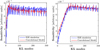 |
Fig. 4. Well-known pyramid sensitivity curves. Left: modulation radius rmod = 2λ/D. Right: modulation radius rmod = 5λ/D. |
We note a small offset between the model and the end-to-end simulations for the low-order modes. This can be explained by the hypothesis of the sliding pupil used in the derivation of the convolutional model. This issue was presented in Fauvarque et al. (2019).
Modal optical gains
We carried out the study by computing modal OG through end-to-end simulations in multiple system configurations. We then compared those OG results to those predicted through the convolutional model. We suppose that we know the turbulence statistics. In other words, we have access to the PSD or the structure function of the residual phases. We focus on how to get this data in a practical way later in this paper.
End-to-end simulations. We proceeded in the following way: Given a PSD, we generated 20 decorrelated phases. We then computed the interaction matrices IMonSky around each of these phases (using a push-pull method) and we used Eq. (7) to compute the OG. The averaged values for each different PSD chosen are presented Figs. 5 and 6; the shaded areas represent the maximum and minimum values found for the OG for 20 phase realisations.
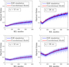 |
Fig. 5. Computed OG on full turbulence screens for multiple r0. The convolutional model fits well with the OG computed by E2E simulations. The shaded area represents the maximum and minimum values found for the OG for 20 phase realisations. Top: rmod = 3λ/D. Bottom: rmod = 5λ/D. |
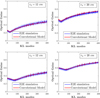 |
Fig. 6. Closed-loop residual phases OG. Number of actuators in the pupil: 20. Top: rmod = 3λ/D. Bottom: rmod = 5λ/D. |
Convolutional model. We used the same PSD used for the end-to-end simulations to compute the IRonSky Eq. (13) and we retrieved the OG thanks to Eq. (14).
We can define two main PSD configurations around which we can compute the OG
-
Full turbulence OG: in this case, the PyWFS works in open loop and wavefront sensing is done on a seeing-limited EM field at the apex of the pyramid. In the vast majority of systems, this is the case for the first loop iteration and before the loop is closed. After a few closed-loop iterations, the EM field seen by the pyramid is no longer seeing-limited because we are in closed-loop operation. We then reach the second configuration described below. Tracking and compensating the OG in the full turbulence can be interesting when the system has convergence issues under strong turbulence or when we want to close the loop using low modulation radii. The results of the comparison for this configuration are given Fig. 5: we note the strong agreement between the convolutional model and the end-to-end simulations.
-
Residual phases OG: the AO loop is closed and the OG are introduced by the imperfect wavefront correction. This case is the most interesting because it can allow us to enhance the closed-loop performance. For this setting, the results are given Fig. 6: we still have a good match between our model and the end-to-end simulations.
By testing our model for various system configurations (multiple modulation radii, multiple r0, and open- or closed-loop residual phases) we demonstrated that the convolutional model can be used to predict the OG with sufficient accuracy to remain in their statistical variability range. It therefore provides a fast and agile way to track OG, provided we have knowledge of the residual PSD. In the next section, we hence focus on how to get this information in a practical way.
3.3. Obtaining the residual PSD
We propose to obtain the residual PSD from the telemetry data. It is a non-invasive method that is already deeply investigated in the PSF reconstruction field (Beltramo-Martin et al. 2019). We note that the residual phase PSD can be split into two parts (Rigaut et al. 1998): the corrected frequencies (area A Fig. 7) and the uncorrected frequencies (area B Fig. 7). These two areas are separated by a deformable mirror (DM) cut-off frequency, which depends on the position and number of actuators. The PSD estimation process works in the following two steps.
-
(1)
By recording the integrated commands sent to the DM, we can assess the shape of the turbulence. In other words, we are able to estimate the Fried parameter r0 and therefore have an estimation of the shape of the PSD outside the correction zone. The estimation of r0 thanks to telemetry data is usually not perfectly accurate and the Fried parameter is often overestimated. However, it has been shown that an AO system can be characterised well to correct for this offset (Fétick et al. 2019).
-
(2)
Recording the residual commands provide information on the residual PSD inside the correction area. This method is not ideal, because all the commands sent to the DM are already tainted by the OG problem. It is possible to overcome this issue using models describing the analytical PSD inside the correction area, provided a simple set of parameters describing the system (Rigaut et al. 1998; Correia et al. 2020).
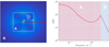 |
Fig. 7. Left: example of a residual PSD for a 40 × 40 actuators system with a Cartesian geometry. In the frequency space, the correction zone is the area labelled A: it is a square with each side of nact = 40/D in m−1. The B area represents the space of uncorrected frequencies. Right: radial cut of the PSD in log scale. |
The next step is to understand what level of accuracy is required when computing the residual phase PSD using telemetry data combined with an analytical model of our system. Using the convolutional model, we propose a brief study to analyse the contribution of the different parts of residual PSD on the OG morphology. As we mentioned earlier, we can split the contribution of the residual phases into two parts: the fitting PSD and the PSD inside the correction zone. It is therefore interesting to study the OG for each of these contributors.
For that purpose we chose two system configurations: an 8 m telescope given a r0 = 15 cm with either 20 actuators (NAOS-like configuration on the VLT) or 40 actuators within the same pupil diameter (SPHERE-like configuration on the VLT: Beuzit et al. 2019). We used the typical residual PSD of these systems to compute the OG thanks to the convolutional model. In Fig. 8, we show the results for which the OG are computed for the full PSD, for the fitting part of the PSD and for the PSD inside the correction area only. For these chosen configurations, it is clear that OG gains are dominated by the energy which lies in the fitting PSD, even for the high-contrast configuration (40 × 40 actuators in the pupil) where the residual energy is equally distributed between the corrected and the uncorrected zone (Fig. 8). Therefore the previous statement often tends to be verified (all the more because we are considering residual phases at the wavefront sensing wavelengths). Yet, it is clear that for a very noisy AO system, the fitting error could be overcome by the error inside the correction zone. In that case, the error on the OG computation is constrained by the estimation of the residual PSD inside the correction zone. Nevertheless, we can conclude that in the vast majority of the observations and for present and future AO systems (the E-ELT will also be in a fitting-error-limited AO configuration), the OG morphology is mainly constrained by the Fried parameter r0, and that the knowledge of this parameter only would suffice to derive a sufficiently accurate model of the OG. Thus, estimating r0 during closed-loop operation is a crucial step for PyWFS OG tracking. To assess the accuracy on r0 that needs to reached, we probe what impact an error in the estimation of r0 has on the computation of OG in Fig. 9. In this plot, and for both configurations studied, we present the maximal acceptable error on the estimation of r0 to maintain an error on computed OG below ±10%. To retrieve OG with an error below ±10%, we see that we need to be more accurate for bad seeing conditions and for AO systems with less DM actuators in the pupil. Overall, the values presented in this figure show that we do not need an incredibly high precision on the Fried parameter to accurately compute the OG using the presented method.
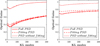 |
Fig. 8. Contribution of the corrected and uncorrected part of a closed-loop PSD (r0 = 15 cm) to the OG. Left: for 20 actuators in the pupil – NAOS configuration. Right: for 40 actuators in the pupil – SPHERE configuration. |
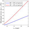 |
Fig. 9. Maximum acceptable error (in percent) on the estimation of r0 to ensure an error on the computed OG under ±10% for two system configurations. |
4. Applying the convolutional model to NCPA correction
The aim of this section is to demonstrate the importance of estimating OGs for the correct control of the AO system by focussing on the specific issue of NCPA correction. The NCPA appear in AO systems when the aberrations between the WFS path and science path are different. In that case, if nothing is done, the AO loop converges towards a flat wavefront on the WFS and the NCPA remain uncorrected on the science camera. This effect can be mitigated by using a non-null wavefront reference target on the WFS, corresponding to the NCPA (Fig. 10). To do so, we propose to proceed with the following three calibration steps:
-
Determination of the NCPA wavefront (using techniques such as phase diversity, for instance Blanc et al. 2003).
-
Computation of the IMcalib around the NCPA wavefront. Because NCPA are not a zero-mean stationary wavefront, they cannot be described by the convolutional model through a structure function as is stated Eq. (13). Furthermore, the diagonal approximation (Sect. 2.3) is not necessarily verified in the case of NCPA. Hence, it is better to calibrate the WFS as close as possible to its working point: the NCPA wavefront.
-
Computation of the WFS response to the NCPA wavefront Icalib(ϕNCPA).
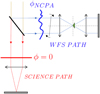 |
Fig. 10. Schematic view of NCPA correction in an AO system. |
Subsequently, the reference WFS intensities correspond to the NCPA. Given a residual phase ϕres, the signal to be reconstructed is then Icalib(ϕres)−Icalib(ϕNCPA). However, using this strategy for PyWFS in presence of residual phase OG is unfortunately problematic and can lead to critical loop instabilities.
4.1. NCPA catastrophe
For a WFS working around its reference position, the signal to be reconstructed is Icalib(ϕres)−Icalib(ϕNCPA). In the case of a classical integral controller, the commands sent to the DM at each frame t is written as
![Mathematical equation: $$ \begin{aligned} c(t) = c(t-1) - G_{\rm temp}\cdot \mathrm{IM}_{\rm calib}^{\dag }\cdot [I_{\rm calib}(\phi _{\rm res}(t)) - I_{\rm calib}(\phi _{\mathrm{NCPA}})] ,\end{aligned} $$](/articles/aa/full_html/2020/12/aa37836-20/aa37836-20-eq18.gif) (16)
(16)
where Gtemp is a diagonal matrix, ideally constituted of the optimised temporal modal gains of the loop. This equation works for a perfectly linear WFS. As previously presented in this paper, the PyWFS exhibits OG. Therefore, the on-sky PyWFS measurements are written as
 (17)
(17)
thus, the Eq. (16) becomes
![Mathematical equation: $$ \begin{aligned} c(t) = c(t-1) - G_{\rm temp} \cdot \mathrm{IM}_{\rm onSky}^{\dag }\cdot [I_{\rm onSky}(\phi _{\rm res}(t)) - I_{\rm onSky}(\phi _{\mathrm{NCPA}})] ,\end{aligned} $$](/articles/aa/full_html/2020/12/aa37836-20/aa37836-20-eq20.gif) (18)
(18)
which gives in the OG diagonal approximation
![Mathematical equation: $$ \begin{aligned} c(t) = c(t-1) - G_{\rm temp}\cdot \frac{\mathrm{IM}_{\rm calib}^{\dag }}{G_{\rm opt}}\cdot [I_{\rm onSky}(\phi _{\rm res}(t)) - I_{\rm onSky}(\phi _{\mathrm{NCPA}})] ,\end{aligned} $$](/articles/aa/full_html/2020/12/aa37836-20/aa37836-20-eq21.gif) (19)
(19)
where Gloop = Gtemp/Gopt is therefore a diagonal matrix used to apply different gains on each of the controlled modes. As we mentioned in the introduction, very efficient methods are available that can optimise this matrix (Deo et al. 2019b), but without differentiating between Gtemp and Gopt. However, it is important to note in this equation that the intensity to be removed is IonSky(ϕNCPA) and not Icalib(ϕNCPA) (see Fig. 11). These two quantities are linked through the following equation:
 (20)
(20)
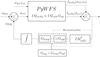 |
Fig. 11. Schematic view of the AO closed loop in presence of compensated NCPA. The feedback loop can be otpimized by computing the quantity Gloop without disentangling Gtemp from Gopt. However, to properly compensate for the NCPA in the forward loop, the value Gopt is needed. |
We see from this equation that we need to get Gopt to be able to properly compensate for the NCPA.
We wondered what would happens if we were just to use Icalib(ϕNCPA) in Eq. (20). To answer this question, we performed end-to-end simulations with the same parameters as before, that is to say for an 8 m telescope with 400 controlled KL modes and a Fried parameter r0 = 15 cm. We chose the H band to be the wavelength of the science path. Because NCPA are usually composed low-order modes, we chose the following arbitrary distribution for the NCPA: a combination of the modes KL5 to KL25, following a f−2 law (see Fig. 12).
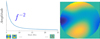 |
Fig. 12. NCPA distribution over a modal basis. NCPA phase chosen for our simulations is a linear combination of 20 low-order KL modes following a f−2 law in rms amplitude. |
We ran several closed-loop simulations while increasing the NCPA amplitudes, and we recorded the Strehl ratio over 16 s of closed-loop integration. The results are given Fig. 15. The dashed line shows the impact of increasing NCPA in the case in which we did not try to compensate for them. When we tried to compensate the NCPA by applying reference intensities on the PyWFS without compensating for the OG, we observed a degradation of performance (Fig. 13). This is not surprising: when subtracting the NCPA reference intensities to the PyWFS measurements, the mode ϕNCPA, i is reconstructed as
 (21)
(21)
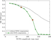 |
Fig. 13. Strehl ratio for increasing NCPA amplitude, in the case of no NCPA compensation and of no OG compensation on the NCPA reference intensities. For NCPA amplitudes that are too while when the reference intensities are not updated with OG, the loop diverges, which we call the NCPA catastrophe. The static aberrations of the two configurations denoted by a red circle are plotted Fig. 14. |
where gopt(ϕNCPA, i) < 1 is the OG associated with the mode ϕNCPA, i, and so we have
 (22)
(22)
This emphasises the fact that if we do not compensate for OG, the reference intensities produce an excess of NCPA proportional to the OG in the loop. This effect is shown Fig. 14 for two cases highlighted by red circles Fig. 15.
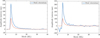 |
Fig. 14. Static aberrations in the AO loop in the case of no OG compensation on the NCPA reference intensities. Left: for NCPA of 70 nm rms. Right: for NCPA of 120 nm rms. |
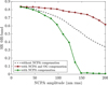 |
Fig. 15. Strehl ratio for increasing NCPA amplitude in the case of OG compensation on the NCPA reference intensities, compared to the previous cases presented before. The performance is increased and the NCPA catastrophe avoided. Nonetheless, a noticeable impact on performance is visible as the NCPA amplitude is increased. |
When the amplitude of the NCPA is sufficiently high, producing too much NCPA creates additional OG that adds to those already generated by the residual phases. By lowering the OG, this leads to an increase of NCPA correction according to Eq. (21). The increase in NCPA correction significantly changes the OG and leads to ever higher NCPA correction levels. This makes the loop diverge, which we label the NCPA catastrophe. We can clearly see this effect in our simulations starting from 130 nm rms and above of NCPA (Fig. 15).
4.2. NCPA compensation using the convolutional model
If we assume the residual phase PSD a known quantity, we can use the convolutional model to compute the OG and to update the reference intensities according to Eq. (20). By doing so, we obtain the upper curve in Fig. 15. Performance is significantly improved, but there is still a built up of static aberrations during the closed-loop operation, preventing the system from maintaining its maximum Strehl ratio irrespective of NCPA amplitude (which would correspond to a flat curve Fig. 15). This can be explained by two phenomena:
-
The way the OG has been defined corresponds to an average state of the system (Eq. (11)). At each frame, the current OG can be higher or lower than the averaged value, introducing an error on the NCPA reference intensities. The ideal strategy would be to have the means to estimate the OG at each frame.
-
The convolutional model characterises the offset between PyWFS measurements when the calibrating around a null-phase and when in the presence of residual phases. But it does not take in account the presence of NCPA in the shape of the computed OG. Therefore, with higher NCPA amplitudes the error on the OG computed with the convolutional model is increased. This explains why performance is decreased with increasing NCPA amplitudes in Fig. 15. Further analysis of this problem is beyond the scope of this paper, but we are currently working on a solution that requires further analytical developments on the convolutional model.
This section highlights the importance of estimating the PyWFS OG for NCPA compensation in closed-loop operation. The OG estimation based on the convolutional model has proven to be efficient for typical NCPA amplitudes (below 100 nm rms) encountered in AO systems. However, handling stronger NCPA amplitudes will require further analytical developments to take into account the modification of OG by the NCPA themselves.
5. Conclusions
The work presented in this paper offers a new method for computing the PyWFS OG. Our approach relies on a physical description of the WFS through a convolutional model, which allows us to analytically compute the impact of residual phases on PyWFS measurements. We have demonstrated the accuracy of this method by comparing results to end-to-end simulations for multiple system configurations.
The presented method requires knowledge of the residual phase statistical characteristics to compute the OG. We presented a practical implementation to estimate residual phase statistics using AO telemetry data in a similar to what is done for PSF reconstruction. We showed that the most important aspect is the knowledge of the turbulence strength through the Fried parameter r0. We also demonstrated that from this r0 parameter alone, a good approximation of the OG could be achieved. In other words, any AO system using a pyramid WFS and capable of providing an on-line estimate of r0 could benefit from estimating the OG using the method we presented in this paper.
Finally, we demonstrated that OG play a crucial part when trying to compensate NCPA with a PyWFS. To avoid what we have labelled the NCPA catastrophe, proper handling of the OG is mandatory. We proposed a way to mitigate the impact of OG on NCPA by computing them using the method we presented in this paper. This work can also be applied to any type of WFS based on Fourier filtering and provides a new insight into the understanding of OG in Fourier-filtering WFS and how to manage these gains.
Acknowledgments
This document has been prepared as part of the activities of OPTICON H2020 (2017–2020) Work Package 1 (Calibration and test tools for AO assisted E-ELT instruments). OPTICON is supported by the Horizon 2020 Framework Programme of the European Commission’s (Grant number 730890). This work was supported by the Action Spécifique Haute Résolution Angulaire (ASHRA) of CNRS/INSU co-funded by CNES. This work also benefited from the support of the WOLF project ANR-18-CE31-0018 of the French National Research Agency (ANR).
References
- Beltramo-Martin, O., Correia, C. M., Ragland, S., et al. 2019, MNRAS, 487, 5450 [NASA ADS] [CrossRef] [Google Scholar]
- Beuzit, J. L., Vigan, A., Mouillet, D., et al. 2019, A&A, 631, A155 [NASA ADS] [CrossRef] [EDP Sciences] [Google Scholar]
- Blanc, A., Fusco, T., Hartung, M., Mugnier, L., & Rousset, G. 2003, A&A, 399, 373 [NASA ADS] [CrossRef] [EDP Sciences] [Google Scholar]
- Conan, R., & Correia, C. 2014, Proc. SPIE – Int. Soc. Opt. Eng., 9148, 91486C [Google Scholar]
- Correia, C. M., Fauvarque, O., Bond, C. Z., et al. 2020, MNRAS, 495, 4380 [CrossRef] [Google Scholar]
- Davies, R., Alves, J., Clénet, Y., et al. 2018, Proc. SPIE, 10702, 107021S [Google Scholar]
- Deo, V., Gendron, É., Rousset, G., et al. 2019a, A&A, 629, A107 [CrossRef] [EDP Sciences] [Google Scholar]
- Deo, V., Rozel, M., Bertrou-Cantou, A., et al. 2019b, Proc. AO4ELT6 [Google Scholar]
- Esposito, S., Pinna, E., Puglisi, A., et al. 2015, in Non Common Path Aberration Correction with Non Linear WFSs, Adaptive Optics for Extremely Large Telescopes 4 – Conference Proceedings [Google Scholar]
- Fauvarque, O., Janin-Potiron, P., Correia, C., et al. 2019, J. Opt. Soc. Am. A, 36, 1241 [NASA ADS] [CrossRef] [Google Scholar]
- Fétick, R. J. L., Fusco, T., Neichel, B., et al. 2019, A&A, 628, A99 [NASA ADS] [CrossRef] [EDP Sciences] [Google Scholar]
- Guyon, O. 2005, ApJ, 629, 592 [NASA ADS] [CrossRef] [Google Scholar]
- Hippler, S., Feldt, M., Bertram, T., et al. 2019, Exp. Astron., 47, 65 [CrossRef] [Google Scholar]
- Hutterer, V., Ramlau, R., & Shatokhina, I. 2019, Inv. Prob., 35, 045007 [CrossRef] [Google Scholar]
- Korkiakoski, V., Verinaud, C., Louarn, M., & Conan, R. 2007, Appl. Opt., 46, 6176 [CrossRef] [Google Scholar]
- Korkiakoski, V., Vérinaud, C., & Louarn, M. L. 2008, in Adaptive Optics Systems, eds. N. Hubin, C. E. Max, & P. L. Wizinowich, International Society for Optics and Photonics (SPIE), 7015, 1422 [Google Scholar]
- Meimon, S., Petit, C., & Fusco, T. 2015, Opt. Express, 23, 27134 [CrossRef] [Google Scholar]
- Neichel, B., Fusco, T., Sauvage, J.-F., et al. 2016, Adapt. Opt. Syst. V, 9909, 990909 [CrossRef] [Google Scholar]
- Ragazzoni, R. 1996, J. Mod. Opt., 43, 289 [NASA ADS] [CrossRef] [Google Scholar]
- Rigaut, F. J., Veran, J.-P., & Lai, O. 1998, in Adaptive Optical System Technologies, eds. D. Bonaccini, & R. K. Tyson, International Society for Optics and Photonics (SPIE), 3353, 1038 [NASA ADS] [CrossRef] [Google Scholar]
- Roddier, F. 1981, Prog. Opt., 19, 281 [CrossRef] [Google Scholar]
- Véran, J.-P., & Herriot, G. 2000, J. Opt. Soc. Am. A, 17, 1430 [NASA ADS] [CrossRef] [Google Scholar]
- Vérinaud, C. 2004, Opt. Commun., 233, 27 [NASA ADS] [CrossRef] [Google Scholar]
- Vigan, A., N’Diaye, M., Dohlen, K., et al. 2019, A&A, 629, A11 [NASA ADS] [CrossRef] [EDP Sciences] [Google Scholar]
All Figures
|
Fig. 1. Diagram of PyWFS, Fourier filtering WFS. A pyramidal mask is placed at a focal plane to achieve optical filtering. The output signal I(ϕ) shows a relationship to the entrance phase ϕ. |
| In the text | |
|
Fig. 2. Panel a: shape of the pyramid mask – arg(m). Panel b: modulation function – w. Panel c: pupil shape – 𝕀p. |
| In the text | |
|
Fig. 3. Sketch of the PyWFS response curve for a given mode ϕi. The push-pull method around a null-phase consists in computing the slope of this curve for a = 0. |
| In the text | |
|
Fig. 4. Well-known pyramid sensitivity curves. Left: modulation radius rmod = 2λ/D. Right: modulation radius rmod = 5λ/D. |
| In the text | |
|
Fig. 5. Computed OG on full turbulence screens for multiple r0. The convolutional model fits well with the OG computed by E2E simulations. The shaded area represents the maximum and minimum values found for the OG for 20 phase realisations. Top: rmod = 3λ/D. Bottom: rmod = 5λ/D. |
| In the text | |
|
Fig. 6. Closed-loop residual phases OG. Number of actuators in the pupil: 20. Top: rmod = 3λ/D. Bottom: rmod = 5λ/D. |
| In the text | |
|
Fig. 7. Left: example of a residual PSD for a 40 × 40 actuators system with a Cartesian geometry. In the frequency space, the correction zone is the area labelled A: it is a square with each side of nact = 40/D in m−1. The B area represents the space of uncorrected frequencies. Right: radial cut of the PSD in log scale. |
| In the text | |
|
Fig. 8. Contribution of the corrected and uncorrected part of a closed-loop PSD (r0 = 15 cm) to the OG. Left: for 20 actuators in the pupil – NAOS configuration. Right: for 40 actuators in the pupil – SPHERE configuration. |
| In the text | |
|
Fig. 9. Maximum acceptable error (in percent) on the estimation of r0 to ensure an error on the computed OG under ±10% for two system configurations. |
| In the text | |
|
Fig. 10. Schematic view of NCPA correction in an AO system. |
| In the text | |
|
Fig. 11. Schematic view of the AO closed loop in presence of compensated NCPA. The feedback loop can be otpimized by computing the quantity Gloop without disentangling Gtemp from Gopt. However, to properly compensate for the NCPA in the forward loop, the value Gopt is needed. |
| In the text | |
|
Fig. 12. NCPA distribution over a modal basis. NCPA phase chosen for our simulations is a linear combination of 20 low-order KL modes following a f−2 law in rms amplitude. |
| In the text | |
|
Fig. 13. Strehl ratio for increasing NCPA amplitude, in the case of no NCPA compensation and of no OG compensation on the NCPA reference intensities. For NCPA amplitudes that are too while when the reference intensities are not updated with OG, the loop diverges, which we call the NCPA catastrophe. The static aberrations of the two configurations denoted by a red circle are plotted Fig. 14. |
| In the text | |
|
Fig. 14. Static aberrations in the AO loop in the case of no OG compensation on the NCPA reference intensities. Left: for NCPA of 70 nm rms. Right: for NCPA of 120 nm rms. |
| In the text | |
|
Fig. 15. Strehl ratio for increasing NCPA amplitude in the case of OG compensation on the NCPA reference intensities, compared to the previous cases presented before. The performance is increased and the NCPA catastrophe avoided. Nonetheless, a noticeable impact on performance is visible as the NCPA amplitude is increased. |
| In the text | |
Current usage metrics show cumulative count of Article Views (full-text article views including HTML views, PDF and ePub downloads, according to the available data) and Abstracts Views on Vision4Press platform.
Data correspond to usage on the plateform after 2015. The current usage metrics is available 48-96 hours after online publication and is updated daily on week days.
Initial download of the metrics may take a while.