| Issue |
A&A
Volume 629, September 2019
|
|
|---|---|---|
| Article Number | A107 | |
| Number of page(s) | 18 | |
| Section | Astronomical instrumentation | |
| DOI | https://doi.org/10.1051/0004-6361/201935847 | |
| Published online | 12 September 2019 | |
A telescope-ready approach for modal compensation of pyramid wavefront sensor optical gain
LESIA, Observatoire de Paris, Université PSL, CNRS, Sorbonne Université, Univ. Paris Diderot, Sorbonne Paris Cité, 5 Place Jules Janssen, 92195 Meudon, France
e-mail: vincent.deo@obspm.fr
Received:
6
May
2019
Accepted:
27
July
2019
The pyramid wavefront sensor (PWFS) is the currently preferred design for high-sensitivity adaptive optics (AO) systems for extremely large telescopes (ELTs). Yet, nonlinearities of the signal retrieved from the PWFS pose a significant problem for achieving the full correction potential using this sensor, a problem that will only worsen with the increasing dimension of telescopes. This paper investigates the so-called optical gain (OG) phenomenon, a sensitivity reduction and an overall modification of the sensor response induced by the residual wavefront itself, with considerable effects in standard observation conditions for ELT-sized AO systems. Through extensive numerical analysis, this work proposes a formalism to measure and minimize the first-order nonlinearity error caused by optical gain variation, which uses a modal compensation technique of the calibrated reconstructor; this enables a notable increase in performance in faint guide stars or important seeing scenarios, for example from 16 to 30% H-band Strehl ratio for a sixteenth magnitude star in r0 = 13 cm turbulence. Beyond the performance demonstrated by this compensation, a complete algorithm for realistic operation conditions is designed, which from dithering a few deformable mirror modes retrieves the optimal gains and updates the command matrix accordingly. The performance of this self-updating technique – which successfully allows automatic OG compensation regardless of the turbulent conditions, and its minimal interference with the scientific instrument are demonstrated through extensive end-to-end numerical simulations, all at the scale of an ELT instrument single-conjugate AO system.
Key words: instrumentation: adaptive optics / techniques: high angular resolution / telescopes
© V. Deo et al. 2019
 Open Access article, published by EDP Sciences, under the terms of the Creative Commons Attribution License (http://creativecommons.org/licenses/by/4.0), which permits unrestricted use, distribution, and reproduction in any medium, provided the original work is properly cited.
1. Introduction
A continuous effort is being provided by the adaptive optics (AO) community to drive forward the usability of the pyramid wavefront sensor (PWFS). Since its introduction (Ragazzoni 1996) as a high-sensitivity alternative to the Shack–Hartmann (Ragazzoni & Farinato 1999; Esposito & Riccardi 2001; Vérinaud 2004), the PWFS has been thoroughly assessed to be the better alternative for high-Strehl AO systems currently in development, including first-light instruments for all three extremely large telescopes (ELTs; Véran et al. 2016; Pinna et al. 2014; Neichel et al. 2018; Clénet et al. 2018).
However, mastering the PWFS for such high-order AO systems comes with a number of theoretical and technological challenges. In particular, the PWFS exhibits a strongly nonlinear behavior, as in-loop residual wavefronts dramatically alter the response of the sensor. This response modification between the calibration and on-sky operations is mainly expressed through a spatial-frequency-dependent sensitivity reduction, a phenomenon named optical gain (OG). Numerical values in median seeing conditions – for example r0 of 14 cm at sensor visible wavelength – for an ELT typically range within 50–80 % of perceived attenuation of closed-loop residuals when compared to small-signal calibrations. Furthermore, the fluctuation of sensitivity with on-sky external parameters prevents a well adjusted subtraction of the calibrated noncommon path aberrations (NCPAs) through the application of the reference slopes, with OG affecting the system as an unforeseen transformation between the acquired setpoint and the runtime measurements. Both the sensitivity reduction and the NCPA alteration are critical and must be addressed to obtain efficient AO with a PWFS.
The PWFS nonlinearities also make the sensor formally incompatible with the usual process of matrix-vector multiplication (MVM)-based phase reconstruction, which is the core of most AO real-time computers (RTCs) today as such linear methods are well proven and computationally efficient. Although analytically extensive models of the PWFS response have been proposed (Shatokhina 2014), and inverse methods to these models are being extensively investigated throughout the AO community (Frazin 2018; Hutterer & Ramlau 2018), our research scopes only within the frame of classical linear reconstruction and sets aside iterative nonlinear methods, so as to avoid the added computational burden. This work was initiated in Deo et al. (2018a).
To handle OG, Esposito et al. (2015) proposed to adjust the overall integrator gain of the AO to compensate for tip-tilt sensitivity in real time. Viotto et al. (2016) suggested to introduce dithering in different modes to assess the dependence of the phenomenon across spatial frequencies. We propose to adapt the RTC control law through a modal gain approach, which depends – among others – on the current seeing, through obtaining a linearization of the PWFS response for variations around AO residuals for a given r0. This approach was initiated by Korkiakoski et al. (2008a), and generalizations based on a generic framework for Fourier-based wavefront sensors are being actively researched (Fauvarque et al. 2016, 2019).
We build upon the OG analysis within the modal command matrix update framework, and derive a compensation method and the necessary technical declinations ensuring its appropriateness for on-sky operations. We numerically investigate the statistical validity of the modal approach and propose a measure-and-update workflow based on a precomputed database of appropriate modal gains. The objective of this research is twofold: to mathematically minimize the nonlinear reconstruction errors within a well-assessed approximation hypothesis; and operationally, to provide procedures that enforce this minimization automatically and continuously, without requiring operator intervention.
We first introduce in Sect. 2 our formalism and hypotheses for optimal and realistic OG modal compensation. Section 3 presents the AO system we use for all simulations in this paper, namely the current design parameters for dimensioning the MICADO single-conjugate AO (Clénet et al. 2018); Sect. 4 validates the statistical hypotheses required, providing a quantitative analysis of sensitivity reduction, optimal gains, and nonlinearity errors and the reduction thereof when applying optimal OG compensation. Section 5 covers the automatic method for optical gain modal coefficients to be updated regularly, using a precomputed database and performing in-situ measurements through an optical dithering of the deformable mirror. Sections 6 and 7 present end-to-end numerical simulations, demonstrating the performance increase using our automatic method and its robustness to turbulence condition variations across a short timescale. Finally, Sect. 8 offers some discussions and results on key points raised with our sky-ready method: optical interaction between dithering and scientific imaging; and appropriate NCPA compensation provided by the improved knowledge of real-time sensitivity.
2. Optical gain: definitions and formalism
2.1. Differential response and interaction matrices
For all analyses and results presented in this paper, our conceptual approach to the PWFS is a generic one of some nonlinear operator between the input wavefront and the normalized pixel space (referred to as slope space hereafter). The Pyr operator covers the transformation between a wavefront ϕ in the entrance pupil and the slope vector S:
where z1, ..., zk are the CCD pixel values for the K valid pixels located within the four pupils re-imaged after the pyramidal prism. The exact expression of the Pyr operator would depend on several parameters, such as PWFS prism defects, misalignments (Deo et al. 2018b), and notably the modulation radius used. This generic formalism could also be extended to WFSs other than a classical four-sided PWFS.
We adopt the global pixel normalization (Vérinaud 2004), and consider all valid pixels (Clergeon 2014) rather than computing the “normalized differences between opposite pairs of pupils” as initially suggested by Ragazzoni (1996). The factor  ensures that the mean value of the slope is 0.25, corresponding to the original definition with a unit flux per subaperture. In Deo et al. (2018b), we demonstrated that this global normalization was more effective in terms of end-to-end system performance than the original local alternative (Ragazzoni 1996); and that using all pixels was altogether equivalent to using the slopes maps, while being the more generic approach, paving the way for the application of the methods presented in this paper to sensors other than an ideal four-faced PWFS as we use herein. The global normalization is also well tailored to locally linearized interpretations of PWFS behavior, such as the studies providing theoretical frameworks consistent with the approach detailed here (Fauvarque et al. 2016; Frazin 2018).
One main step for the calibration of the AO system is to obtain the interaction matrix as a linearization around the operating point. Here, we consider the behavior of the PWFS with some residual phase error due to the AO loop ϕRes. This can be done with sufficiently small deformable mirror (DM) modal pokes ϵ.ϕ and disregarding noise; one then obtains the derivative of the PWFS response along a wavefront ϕ locally around ϕRes:

The interaction matrix at ϕRes: dPyrϕRes is then a collection of differentiations dPyr (ϕi; ϕRes)1 ≤ i ≤ N for the modal basis (ϕ1, ..., ϕN) of the DM wavefront space. The modal basis to be used is usually determined beforehand based on criteria other than OG compensation, and is beyond the scope of this paper. We simply assume here the use of a nonredundant basis reduced to a convenient subset of the DM space, free from any PWFS blind modes.
Among these generically defined interaction matrices, the one around the unaberrated wavefront ϕRes = 0 holds a specific function as the one that is effectively computed and used to calibrate the AO. When analyzing OG quantitatively, it is observed that ϕRes = 0 yields the maximum PWFS sensitivity. Therefore, we have taken the reference interaction matrix dPyrϕRes = 0 as a uniquely defined comparison point for relative assessments of OG impact.
From dPyrϕRes = 0, the wavefront reconstructor of the PWFS is obtained:
where •† is appropriately conditioned matrix generalized inversion. The above defined Rec is effectively the modal command matrix of the system in the usual acceptance for the selected DM basis, and the reconstruction is exact for a sufficiently small wavefront ϕ generated by the DM:
2.2. Optical gain: a turbulence-induced nonlinearity
The reconstruction identity of Eq. (4) generally does not hold in realistic AO operation conditions when a non-negligible wavefront aberration reaches the PWFS. This induces a variation in the PWFS response, this variation being important even when the residual is dominated by the fitting term. Such a situation is illustrated through a preliminary example in Fig. 1, displaying the slopes S (ϕ) when the PWFS is shown a tilt aberration, with and without an added 120 nm RMS fitting ϕRes (top); and the response curves for a few modes (bottom). This class of effects is what we name the OG phenomenon: an invalidation of the calibrated response of the PWFS due to residual wavefronts, a characteristic not covered by the calibration.
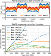 |
Fig. 1. Top: PWFS slopes vector for a flat wavefront, a 300 nm RMS tilt, and the same tilt added to a 120 nm RMS fitting error wavefront ϕRes, showing the attenuation of the signal. Data are smoothed by a window of 50 samples in width for clarity. Bottom: recorded PWFS response curve to three modes – tilt and Karhunen–Loève 20 and 3000 – with and without the same ϕRes. The tilt curve without residuals saturates around 750 nm RMS. The AO setup simulated is described in Sect. 3. |
Mathematically, Eq. (4) failing even for small ϕ signifies that the Jacobian dPyrϕRes near the residual wavefront differs from the calibrated dPyrϕRes = 0, and therefore that the linear reconstructor Rec is inappropriate for the AO operating regime. In order to overcome this issue which impedes the linear wavefront reconstruction framework, one would ideally always use the appropriate command matrix, provided the instantaneous disturbing wavefront ϕRes is known. Such continuous measurements and updates of  are unfortunately conceptually and computationally unreasonable.
Modal OG compensation – initiated by Korkiakoski et al. (2008a) – is a first-order approximation and substitutes the estimation of the instantaneous Jacobian by a modal scaling of the reference interaction matrix, assuming modal optical gain coefficients (OGCs) may be obtained. For this operation to be possible, the required property is that for each DM basis mode ϕi (1 ≤ i ≤ N), a scalar λi exists such that:

or, spanning the whole basis, for a diagonal matrix ΛϕRes = Diag (λ1, ..., λN) to exist such that

With Eq. (6) verified, the modal command matrix of the system can be updated with  , that is, with a line-wise rescaling with the candidate OGCs – ignoring for now cases with ill-conditioned ΛϕRes. Assuming that Λ matrices can be found that are suitable for most AO operating conditions, this analysis paves the way for an appropriate OG compensation through regular command matrix updates.
2.3. Defining the optimal optical gain coefficients
Equation (6) nonetheless represents a strong hypothesis in the general case, and therefore we propose a phenomenological approach to quantify the discrepancy between dPyrϕRes and dPyrϕRes = 0 ⋅ ΛϕRes for optimally adjusted λi. Our strategy to calibrate optimal OGCs is hence to evaluate the impact of residual wavefronts on DM basis modes, and thereupon to derive the optimal OGC for this mode.
For a DM wavefront ϕ, represented as vector  on the DM basis ϕ1, ... , ϕN, we consider the OG-uncompensated small-signal reconstruction near a residual wavefront ϕRes:

The vector dϕRes is the DM space wavefront reconstructed from PWFS measurements, erroneously instead of c. We choose to decompose it into components colinear and orthogonal to c:
as illustrated in Fig. 2. From this decomposition, we bring out the colinear sensitivity reduction coefficient, which traces the core effect at the origin of the denomination “optical gain”. This is expressed as:
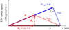 |
Fig. 2. Schematic OG-impeded reconstruction of a mirror mode |
with ||•|| being wavefront euclidean norm. Similarly, we define the orthogonal nonlinear coefficient:
as an indicator of the confusion between DM modes arising from the PWFS nonlinear response.
From α∥ and α⊥, we derive the putative optimal OGC for wavefront ϕ:
as the minimizing solution for the first-order nonlinearity error ||c − Gopt (ϕ; ϕRes)×d||. The original error using the reconstructor Rec is denoted eRec = d − c, and the minimized one eOpt = Gopt × d − c; their normalized lengths are simply expressed from α∥ and α⊥:

The quantitative values of eOpt and eRec – and the statistical distributions thereof – are investigated numerically in Sect. 4.2, and prove to be very useful indicators to quantify first-order nonlinearity errors when using appropriate OGCs.
To obtain optimal OGCs for all controlled modes ϕi of the DM basis, Eqs. (7)–(11) are applied for each ϕi. Equation (2) describes the way dPyrϕRes is computed in our simulations, by freezing the AO loop on a given ϕRes and introducing small perturbations ϵ.ϕ around it. Using this evaluation of dPyrϕRes, we may then derive the quantities of Eqs. (7)–(11). The reconstructor update diagonal matrix  is defined by its diagonal coefficients Gopt (ϕi; ϕRes)1 ≤ i ≤ N.
2.4. Statistics with disturbing wavefronts
In Sect. 2.3, we obtained a candidate set of optimal OGCs given a residual wavefront ϕRes. At the current state of this research, it is unrealistic to measure Gopt (ϕi; ϕRes) for every single turbulent wavefront realization; therefore, it is useful to define classes of realistic closed-loop wavefronts yielding similar Gopt (ϕi; ϕRes). This objective is the direct consequence of a key requirement for modal OG compensation with regular command matrix updates to perform: OGCs are to be valid for a sufficient duration between updates. Originally, Korkiakoski et al. (2008b) proposed that OGCs were only dependent on the current r0 of the turbulence. It turns out that during the writing of this article, Fauvarque et al. (2019) came up with the analytical demonstration that within a convolutional model of the PWFS, Eq. (6) is exact with Λ depending only on the phase structure function of the wavefront residual.
Upon this prior, we perform a classification of wavefronts of interest with a single quantitative parameter: we define a wavefront class to be the set of wavefronts that share an identical spatial power spectrum density (PSD). Among these infinite classes, only the ones that are realistic to an AO system are of relevance, which we parameterize by a single scalar p0.
The wavefronts of class p0 shall be the ones with the PSD corresponding to a fitting error of Fried parameter r0 – null power up to the DM cutoff frequency and von Kármán spectrum beyond – added to some typical residuals over the DM modes covering aliasing temporal and nonlinearity error budgets. We therefore reduce the class parameter p0 to the Fried radius r0. The notation p0 is meant to negate any potential ambiguity between the Fried parameter of the turbulence and the coefficient used for computing OGCs when presenting results further in this paper, although underlining the conceptual connection in between. While r0 is a physical parameter, p0 is merely a descriptive label for statistical classification purposes. The relative composition of the residuals is computed in this paper through preliminary end-to-end simulations of the AO system, which did not simulate noise.
For analyzing the statistical properties of the indicators defined in Sect. 2.3, we now consider α∥, α⊥, Gopt (ϕi; p0) for each ϕi as scalar random variables depending on the turbulent realization ϕRes with p0-parameterized PSD, and eRec and eOpt as vector random variables. For a unified notation, we refer to their averages and standard deviations over the p0 wavefront class as μ[•(ϕi;p0)] and σ[•(ϕi;p0)], respectively. Numerical analyses regarding the significance of these indicators and their behaviors across p0 classes are presented in Sect. 4.
3. Adaptive optics simulation setup
Advancing in our developments requires numerical simulations, and this section presents the AO simulation setup used for all numerical simulations presented in Sects. 4–8. Parameters of the simulation are synthesized in Table 1; the PWFS samples the wavefront over 92 pixels across the pupil diameter, at an R-band median wavelength of 658 nm. To devise significant methods and provide results meaningful to the ELT instrumental projects, we considered parameters close to those of the MICADO SCAO design (Vidal et al. 2017), in which it was in particular demonstrated that a single modulation radius within the 3–5 range provided maximum performance at all guide star magnitudes. Given this prior, the modulation radius is henceforth considered as a design parameter and not as an optimization degree of freedom.
AO numerical simulation parameters.
The telescope pupil is the ESO-defined ELT model, although with spiders omitted; the DM is the latest known model of the adaptive mirror M4 of the ELT (Biasi et al. 2016), with a hexagonal pattern of pitch 54 cm in M1 space, simplified with a spatially localized influence function model with a coupling of 0.24. All numerical simulations were performed using the COMPASS (Ferreira et al. 2018a) simulation package, running on a Nvidia DGX-1 server equipped with two 20-core Intel Xeon E5-2698 processors and eight Nvidia Tesla P100 graphics boards. Generating a 4 modulated PWFS image on this server typically requires 60–70 ms.
4. Modal analysis of compensation coefficients
4.1. Sensitivity reduction and optimal gain
This section presents results from numerical simulations regarding the dependence of α∥ and Gopt with turbulence residual amplitude as characterized by p0. Results shown are extracted from the abacus precomputed for our simulated ELT AO – a process covered in detail in Sect. 5.2, which is obtained averaging interaction matrices dPyrϕRes (Eq. (2)) for 15 different ϕRes, at each of 15 p0 values log-spaced from 4.0 to 35.0 cm. These results provide the required consistency check of the key hypotheses allowing optical gain modal compensation: for a well chosen set of modes, p0 is a parameter that effectively induces values that are stable with the phase realization ϕRes; results in this section demonstrate that the Karhunen–Loève (KL) basis fits such a criterion. Stability here is meant in the sense that the standard deviation measured across the wavefronts of a p0-labeled class is negligible compared to the variations of the gains with p0, both for the sensitivity loss α∥ (ϕi; p0) – as shown in Fig. 3 – and the optimal gain Gopt (ϕi; p0) – shown in Fig. 4. This is shown respectively in Figs. 3 and 4, with the shaded areas showing ±2 standard deviations around the solid line showing the average μ[α∥] or μ[Gopt]. The constant thickness of the σ bar in logarithmic scale suggests a rough proportionality between σ and μ.
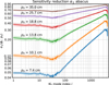 |
Fig. 3. Subset of the α∥ abacus data. Solid lines: μ[α∥ (ϕi;p0)]; shaded areas: ±2σ[α∥ (ϕi;p0)], as computed numerically on 15 independent wavefronts of class p0 in conditions of Table 1, except that no noise is introduced. Curves are smoothed for improved clarity using an adaptive recursive filter with window width log (i). |
All measured values demonstrate the stability of the measurement α∥ for a given p0, with relative standard deviations ![$ \dfrac{\boldsymbol{\sigma}\left[\alpha_{\parallel}\,(\phi_i;\ p_0)\right]}{\boldsymbol{\mu}\left[\alpha_{\parallel}\,(\phi_i;\ p_0)\right]} $](/articles/aa/full_html/2019/09/aa35847-19/aa35847-19-eq23.gif) below 3% for all p0 > 7.4 cm, and the possibility of high-confidence estimations of p0 using only α∥ (see Fig. 3) – a feature that we look for in Sect. 5. Numerical values are also insightful on the important impact of OG on sensitivity: even in extremely good seeing conditions, losses in sensitivity relative to the calibration of 30 − 45% are to be expected (p0 = 25.7 cm in Fig. 3). At the near-median value p0 = 13.8 cm, low-order modes are attenuated by a factor of 5, and at the extreme p0 = 7.4 cm by a factor of more than 20.
below 3% for all p0 > 7.4 cm, and the possibility of high-confidence estimations of p0 using only α∥ (see Fig. 3) – a feature that we look for in Sect. 5. Numerical values are also insightful on the important impact of OG on sensitivity: even in extremely good seeing conditions, losses in sensitivity relative to the calibration of 30 − 45% are to be expected (p0 = 25.7 cm in Fig. 3). At the near-median value p0 = 13.8 cm, low-order modes are attenuated by a factor of 5, and at the extreme p0 = 7.4 cm by a factor of more than 20.
The sensitivity reduction is well described by two trends, below and above the modulation radius spatial frequency, corresponding for 4 to KL mode 30. The sensitivity loss below this index is homogeneous, then increasing beyond this index up to maximal values for the highest orders. For modes ϕi (30 ≤ i ≤ 3000), for which spatial frequencies are entirely within the DM resolution, the sensitivity reduction coefficient follows a p0-dependent power-law trend. For ϕi (i > 3000) modes tend to resemble waffle modes rather than atmospheric KL modes – due to the DM resolution limit– and this induces more chaotic variation between modes, nevertheless without compromising the stability at a given p0.
The optimal gain Gopt to apply in p0-PSD wavefront conditions is shown in Fig. 4. It generally behaves as the inverse of α∥, yet with a more discrete cutoff at the modulation radius, the knee being smoothed out by the relative weight of α⊥ (Eq. (11)) and the desired minimization of ||eOpt|| (Eq. (12)).
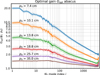 |
Fig. 4. Subset of the Gopt abacus data. Solid lines: μ[Gopt (ϕi;p0)]; shaded areas: ±2σ[Gopt (ϕi;p0)]. Data computed and smoothed as in Fig. 3. |
Extensive numerical analyses and comparisons for various DM bases and PWFS modulation radii are not covered in this paper, but were documented in previous work (Deo et al. 2018a). We showed in this latter publication that the overall sensitivity, with α∥ factored in, is independent of the modulation radius for modes bearing frequencies past the modulation-induced cutoff, while smaller modulations provide greater sensitivity for low-order modes below this cutoff. This sensitivity analysis has to be considered alongside dynamic range effects, and an optimal trade-off has been highlighted near the chosen 4 (Vidal et al. 2017).
Regarding modal basis choices, it was shown that both the Fourier and KL DM bases provide extremely stable α∥ (ϕi; ϕRes) values at a given p0, unlike the natural actuator basis which proved to be unsuitable for an OGC approach. When comparing α∥ numerical values between Deo et al. (2018a) and this paper, data shown here are smaller for an identical p0 parameter. This difference is well explained by first: the upscaling of the AO system considered (18–39 m diameters); and second, the redefinition of the p0-class PSD, which now includes DM space loop residuals instead of being restricted to a fitting error wavefront.
4.2. Nonlinear reconstruction errors
Along with computing α∥ and Gopt in a variety of conditions, we extract the reconstruction error incurred by DM modes with and without OGCs (resp. eOpt and eRec), as defined in Sect. 2.3 and depicted in Fig. 2. We reiterate that ||eOpt|| and ||eRec|| are the RMS errors for each mode of the command matrix Rec compared to the OG-disturbed effective reconstruction, with and without an OGC applied. Numerical values for ||eOpt|| and ||eRec|| are shown in Fig. 5, restricted to three p0 values of 7.4, 13.8, and 25.7 cm for clarity.
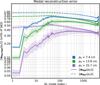 |
Fig. 5. Error terms with and without applying static Gopt (ϕi; p0) OGCs. Solid lines: μ[||eOpt (p0)||] (with OGCs); dashed lines: μ[||eRec (p0)||] (without modal compensation); shaded areas: ±2 standard deviations. Data computed and smoothed as in Fig. 3. |
The error term without OGCs eRec allows for a quantitative analysis of the potential impact of OG on AO performance. Below the modulation radius cutoff, μ[||eRec||] is shown to have an approximately flat magnitude of resp. 0.5, 0.8, and 0.95 – in units of the input magnitude ||ϕi|| – for p0 values of 25.7, 13.8, and 7.4 cm. Beyond the cutoff, μ[||eRec||] slowly decreases – altogether by 25–30% for the highest order modes. These surprisingly high values underline that using the calibrated command matrix Rec along with an analytically derived integrator gain would not permit an appropriate control of the PWFS, even in very favorable seeing conditions.
The ||eRec|| metric alone is insufficient to distinguish the colinear, OGC-compensable error c − d∥ and the confusion portion d⊥; the optimally reduced reconstruction error ||eOpt|| sheds light on this repartition. For high frequency modes, ||eOpt|| shows only a moderate reduction over ||eRec||, from which is understood that a significant OG confusion between modes occurs. A value of  for ||eOpt|| corresponds to α⊥ = α∥, i.e., an equal weight of the sensibility and the nonlinear confusion. This value is seldom reached, that is, only for mid-order modes when p0 = 7.4 cm.
The reconstruction error is significantly reduced for modes below the modulation cutoff, with data showing that the orthogonal component increases with spatial frequency, yet that most of the error is borne by the colinear term; this significant reduction is observed regardless of atmospheric conditions. Noticeably, the optimally reduced error is minimal for the tip-tilt modes, with an error norm reduced by a factor 5–8, for example from 0.80 down to 0.10 for median conditions p0 = 13.8 cm.
The error reduction for modes which bear the most power in the turbulence demonstrates that OG can be well corrected using modal OGCs, with a significant reduction of the nonlinearity error budget to be expected. It should be noted however that while μ[||eOpt||] is indicative of the nonlinear behavior of each mode, it should not be directly interpreted as a nonlinearity error budget, but merely as an initial step towards its derivation.
5. Leveraging the OG analysis for AO operations
So far, we have derived an analysis in Sect. 2 to obtain error-minimizing rescaling coefficients for each mode – by applying Eqs. (2) through (11) – in order to update the PWFS command matrix with
![$$ \begin{aligned} \mathbf Rec \,(p_0) = \mathrm{Diag} \left(\boldsymbol{\mu }\left[G_{\mathrm{opt}}\,(\phi _i; p_0)\right],\ i \in [1,\ N]\right) \cdot \mathbf Rec . \end{aligned} $$](/articles/aa/full_html/2019/09/aa35847-19/aa35847-19-eq27.gif)
However, this methodology, which is hereafter referred to as static OGCs, promptly reaches limitations when its applicability is considered beyond a laboratory setup – as the on-sky turbulence cannot be halted to compute an interaction matrix as per Eq. (2). It is only properly adequate if the residual PSD matches the partially corrected turbulence chosen for the p0 = r0 wavefront class – which may not be the case due to the varying relative weights of nonlinearity, latency, and noise error budgets. Furthermore, it requires an adequate estimate of the current atmospheric Fried radius r0, obtained via a yet-to-be-defined method of AO telemetry – which will have to face the challenge posed by the fact that pseudo-openloop wavefronts cannot be estimated through the PWFS due to OG itself.
5.1. Automatic method for determination of optical gain coefficients
For AO operations, we set the objective to propose a sky-ready, fully automated method that proposes an answer to the two shortcomings mentioned immediately above. This algorithm proceeds to obtain sensitivity reduction statistics through dithering some DM modes. From there, it deduces the operating conditions through the parameter p0, and then extrapolates corresponding Gopt values for all DM modes from a precomputed database. Our objective in designing this method is twofold: First, implement a near real-time, efficient compensation of PWFS nonlinearity. Second, propose an algorithm that enforces OG compensation automatically, in all expected conditions at the telescope, and that exonerates the operator from any kind of fine-tuning of one or many AO control parameters so as to obtain the maximum performance.
Using a sinusoidal dithering followed by a synchronous demodulation stands as a natural approach to this problem. Deformable mirror dithering has often been used to retrieve in-situ values of a variety of turbulence-dependent measurements (Rigaut et al. 2010), or on-sky interaction matrices (Esposito et al. 2006; Kolb et al. 2012). Dithering, coupled with synchronous demodulation (Sect. 5.3), allows for an optimized retrieval of the desired information α∥ using fine-tuned parameters for this purpose; in particular the frequency range and the desired S/N – as is detailed in Sect. 5.4.
Using DM dithering however adds an intrusiveness issue between the science and the AO channels, as dithered signals are forwarded to the scientific instrument. We seek to introduce the minimal disturbance to the science channel while satisfactorily tracking OG fluctuations. Design strategies include using minimal dithering amplitudes, a well-selected minimal number of modes, and reduced active duration, possibly synchronized by the instrument control system with short periods of offline science time. Dithering signal parameters and design trade-offs are presented in Sects. 5.3 and 5.4, and numerical simulation results on the intrusiveness of the automatic OG compensation into the scientific imaging are presented in Sect. 8.1.
5.2. Database computation
Database computation is a step that comes offline, well before any on-sky operations and ideally during the commissioning of the instrument. This is entirely done by end-to-end numerical simulations configured to match the optical setup, and consists in populating a database with OGCs.
For each sampled p0 parameter within the range of interest – in our case 15 values sampled from r0 = 4.0 to 35.0 cm at 500 nm, a number of wavefronts are generated with the selected p0-class closed-loop wavefront PSD, defined using the method described in Sect. 2.4. An interaction matrix is computed around each of these wavefronts as per Eq. (2), allowing statistically converged target values μ[α∥ (ϕi;p0)] and μ[Gopt (ϕi;p0)] to be to computed for all p0 and all DM modes ϕi, as already presented in Figs. 3 and 4. These two compiled p0-labeled abacuses will allow the interpolation and gain retrieval process described in Sect. 5.5. Such abacuses must be computed for all determined operating modes of the system, with noticeably different values and structure for different modulation radii; otherwise, they remain unchanged for the lifetime of the system, as they are mostly dependent on the sampling of the DM and WFS, their relative positioning, and the modulation radius. We compute abacuses with a simulated star bright enough to disregard noise, and we use the same abacus during operations regardless of the guide star being observed.
5.3. Dithering sequence
The dithering sequence now happens on-sky during observations. Our strategy is to use a cosine-wave pseudo-openloop dithering of the DM to retrieve the amplitude seen by the PWFS. For a subset of K modes ψ1, ..., ψK of the DM, a cosine-shape excitation is introduced for a total added amplitude to the AO loop integrator output at time step t of:
where Ai and fi are the a priori determined dithering amplitudes and frequencies for each of the ψi modes. From the recorded PWFS slopes S (t) during the same time frame – re-synchronized from latency effects, we demodulate the seen amplitude of the ψi modes at frequencies fi in terms of the reference reconstructor Rec. For the current α∥ (ψi), this quantity estimates
![$$ \begin{aligned} \alpha _{\parallel }^\star \,(\psi _i) = \dfrac{1}{A_i}\dfrac{1}{T}\dfrac{1}{||\psi _i||^2}\left|\sum _t \cos \,(2\pi f_i t)\times \left[\psi _i \otimes \left(\mathbf Rec \cdot {\boldsymbol{S}}\,(t)\right)\right]\right|, \end{aligned} $$](/articles/aa/full_html/2019/09/aa35847-19/aa35847-19-eq29.gif)
with starred values denoting measured or estimated values, ⊗ the inner product in wavefront space, and T the duration of the sequence in samples. A typical example of dithering sequence and signal retrieval is shown in Fig. 6, with the input amplitude dithered Ai × ||ψi|| × cos (2πfit), the true signal on the PWFS, and the reconstructed modal signal as used in Eq. (15): ||ψi||−1 × ψi ⊗ (Rec⋅S (t)). More generally, signals other than a cosine can be used, and demodulated using cross-correlation in place of Eq. (15).
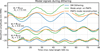 |
Fig. 6. Typical example of a dithering sequence, as we use for all numerical simulations using the dithering method in this paper. “DM dithering”: ψi amplitude injected Ai × ||ψi|| × cos (2πfit); “Mode ampl. on PWFS”: true instantaneous component in ψi of the wavefront; “PWFS reconstruction”: ψi component measured from the slopes, i.e., ||ψi||−2 × ψi ⊗ (Rec⋅S (t)). For this case, the turbulence r0 is 14.5 cm, with conditions of Table 1 but no noise. Wavefront maps of the ψi are shown in Fig. 7. Data for ψ1 and ψ3 are offset by +20 and −20 nm, respectively. |
5.4. Dithering sequence design and parameters
For an efficient performance of the automatic update method, suitable amplitudes, frequencies, mode choices, and so on have to be determined for the AO system. Possible choices are numerous and there are no unique acceptable solutions. We reached a satisfactory solution through trial and error on simulated systems of different sizes and now describe the retained decisions and the various trade-offs considered. The choices of parameters for the dithering sequence used throughout this project, according to the constraints detailed hereafter, are synthesized in Table 2.
Parameters used for the dithering signals.
Obtaining open-loop slopes. The computation of Eq. (15) is an appropriate estimator if closed-loop rejection of the dithering signal can be ignored. To access a relevant value for  , the AO system consequently behaves in an open-loop mode, albeit in the small-phases approximation such that rejection of the dithering signals can be ignored. However, completely filtering out ψi modes from Rec during the dithering allows the atmospheric component to build up to nonsmall quantities. Therefore, we choose to reduce the modal gains of the K modes ψi by a factor of 8.0 during the dithering sequence, while all nondithered modes are maintained in nominal closed-loop regime.
Frequencies. Sufficiently low frequencies fi are to be chosen so as to be well within the bandwidth of the DM, and below the overshoot band of the feedback loop – as a small amount of the dithered signal will be injected into all modes through nonlinear cross-coupling, and will possibly be amplified by the overshoot as all other modes than the ψi are still operated in close-loop. Operating well beneath the Nyquist frequency is also meant as a conservative strategy for real AO systems, considering the possibility of fluctuating, fractional delays, and possible difficulties for characterization of DM and telescope control transfer functions close to the Nyquist limit.
Beneath these upper bounds, fi should be as high as possible in order to escape the massive low-frequency spectrum of the turbulence and mitigate the impact of lengthy drifts from the closed loop value on the scientific imaging path. Given that we operate our AO loop at 500 Hz, with an overshoot band centered on 50 Hz for a two-frame delay integrator RTC, we select fi frequencies in the range 20–40 Hz. To avoid fratricide effects between the ψi due to the unknown d⊥ OG cross-coupling, we select different, evenly spaced frequencies for all ψi within this range. We ought to have avoided choosing harmonic frequencies, but frequency-mode analyses showed that this issue was insignificant given the chosen ψi. The fi values are conservatively within the ELT M4 flat (±1 dB) response band of 200 Hz (Sedghi et al. 2010).
Amplitudes. Dithering amplitudes Ai must on the one hand remain small enough as to not perturb the science imaging quality during the dither sequence, yet be large enough to obtain a high-confidence measurement of  . In order to always use appropriate Ai, we perform an automatic S/N assessment immediately before the dithering sequence. The gains for ψi are also divided by 8.0 during the same duration, and the noise level is assessed in frequencies within Δf of fi through:
![$$ \begin{aligned} n_i = \dfrac{1}{2\Delta f}\dfrac{1}{T}\dfrac{1}{||\psi _i||^2} {\int }_{f_i-\Delta f}^{f_i + \Delta f} \!\left|\sum _t \cos \left(2\pi f t\right)\left[\psi _i \otimes \left(\mathbf Rec \cdot {\boldsymbol{S}}\,(t)\right)\right]\right|\mathrm{d} f, \end{aligned} $$](/articles/aa/full_html/2019/09/aa35847-19/aa35847-19-eq32.gif)
typically using Δf such that it covers a few Fourier transform bins. From this measured ni noise floor at frequency fi in mode ψi, the amplitude Ai is obtained relative to a set target S/N of 5 for a lower range α∥ of 0.1, hence:

Finally, to avoid exceptional situations in very high or low S/N, Ai is clipped to extremal values such that Ai × ψi amounts to between 1.5 and 25.0 nm of spatial RMS.
Choice and number of modes. In order to obtain estimates of  while properly sampling the spatial frequency range, it is appropriate to choose a large enough number of modes to span the entire DM basis, with minimal d⊥-induced cross-coupling. Conversely, a minimal number of modes guarantees a reduced total wavefront disturbance during the dithering period – both from the uncorrected atmospheric drift and the dithering signal itself. In order to evaluate this compromise, we started with a choice of K = 20 modes, evenly sampling the frequency plane, and gradually monitored the performance while reducing K. A consistent performance of the procedure was validated down to K = 3 dithered modes.
The three retained KL modes ψ1, 2, 3 for the ELT-M4 setup we use for numerical simulations are shown in Fig. 7, along with their spatial PSD. An important criterion for the choice of a mode is to ensure that its PSD energy is well distributed azimutally in the frequency plane, which ensures that science path speckles induced by the dithering signal are diluted over a larger area in the focal plane, rather than building very localized artifacts. Also, the pseudo-openloop drift should not impede imaging, hence the choice of ψ1 with frequency contents of the order of  . This is low enough to extrapolate the gains of the first optical modes with confidence, yet high enough to leave the Airy core and the first few rings unaltered.
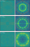 |
Fig. 7. Wavefront maps (left column) and log-scaled spatial PSD (right) for the dithered modes ψ1, 2, 3. The displayed area is 39.5 m across for wavefront maps and |

Duration of dithering. The last design parameter to discuss is the duration of the dithering sequence; it must be long enough to achieve the target S/N given by Eqs. (16) and (17), yet not impede the general workflow of the AO operation. We opted for 500 msec, i.e., 250 frames at 500 Hz. As discussed in Sect. 8, this duration is well suited to induce very low dithering amplitudes in most situations, and can be well integrated into scientific operating procedures.
5.5. Interpolation and retrieval of optical gain coefficients
With  values obtained from demodulating the recorded dithering sequence for three modes, the algorithm proceeds to define appropriate
  values for all DM modes. This process is done in three steps, which are depicted with simulation data in Fig. 8.
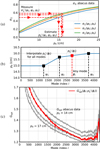 |
Fig. 8. Successive steps of the abacus-based interpolation process. (a) For each of the K dithered modes ψi, the measurement |


For dithered modes ψi, the sensitivity reduction coefficient  is mapped to a
  value using the α∥ abacus. This measured
  is representative of the turbulence power in spatial frequencies borne by mode ψi. As the residual spectrum does not necessarily match the PSD chosen for a given p0 wavefront class, it is expected that
  would differ across dithered modes. From the measured values
  , a value is interpolated for all modes using a linear interpolation across the spatial-frequency-sorted natural ordering of the KL modes, and extrapolating with
  (resp.
  ) for modes with indexes below ψ1 (resp. beyond ψ3).
Finally, the Gopt abacus is used to obtain putative  for all modes, interpolating from the precomputed p0 values. The command matrix of the system can now be updated using these OGCs, to be maintained until the next OGC update sequence occurs.
5.6. Additional weighting of optical gain coefficients
When using either static OGCs – that is, Gopt (ϕi; p0 = r0) assuming r0 is known – or automatic OGCs, that is those obtained through regular dithering and updating sequences, a nefarious effect arises; this is observed when the scalar integrator gain is overset beyond some reasonable value ensuring stability, particularly in above-median seeing conditions with bright guide stars. Updating the RTC with Gopt coefficients sets all modes to a comparable level of optimum rejection; if the scalar integrator gain is then overset, the lowest-order modes – bearing the most residual and being the most boosted by OGCs (Fig. 4) – enter first in an oscillatory regime characteristic of a lack of stability. In particular, the tip-tilt are the most affected modes and the science image suffers from jittering and is rendered unexploitable. The same effect occurs if r0 increases by a significant fraction between two dithering sequences, with the experienced OG sensitivity reduction becoming less dramatic, hence a response from the loop equivalent to that caused by a gain increase. This effect was observed in our simulations, and is discussed in more depth in Appendix A; it was deemed to be a critical shortcoming for system robustness, and therefore we devise a workaround to prevent low-order instability.
We circumvented the issue by adding an additional weighting to the Gopt coefficients, allowing us to control which modes enter oscillatory regime first when an unexpected gain increase occurs. For all results when referring to weighted OGCs, we add an additional modal gain multiplier of:
where i is the mode index and N the total number of modes. Numerical parameters were fine-tuned with the experimental ELT setup described in Sect. 3, yet were tested and should be appropriate on other designs as long as a DM-reprojected KL basis ordered with increasing spatial frequencies (Ferreira et al. 2018b) is used. The weighting function is plotted in Fig. 9, along with a map of this weighting distribution in the Fourier plane.
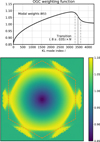 |
Fig. 9. Top: corrective OGC weighting W(i), as defined per Eq. (18), for the ELT simulation with N = 4309 modes. Bottom: distribution of the weighting W(i) in the Fourier plane of the pupil. At each frequency in the Fourier plane, the weight shown is the W(i) of the KL mode which bears the most energy at that specific frequency. This representation is obtained by computing the Fourier transform of all modes and finding the mode that is most representative of any given spatial frequency. The dashed hexagon shows the correction zone of the M4 DM. The displayed area is 100 |

Equation (18) corresponds to a square-root shape from 0.85 at lowest orders to 1.15 at highest orders, with the arctan term bringing W(i) back to 1 across a transition of width 0.035 N centered on mode number 0.8 N. A square root function corresponds to a linear increase with the norm of the spatial frequencies borne by the mode. The arctan term is introduced to cut-off the gain boost before the highest-order waffle-like modes at the end of the KL DM basis. These highest-index modes have spatial PSDs well localized on the corners of the DM rejection domain, and therefore they quickly induce undesirable artifacts in the point spread function (PSF) when reaching oscillatory regimes.
Boosting the gain of mid-order modes ensures that if for any reason some instability is approached, mid-order modes would be affected first. Low orders, and tip-tilt in particular, would be shielded, as well as waffle-like modes: the additional mid-frequency wavefront perturbation will in turn induce a reduction of the PWFS sensitivity, providing a self-stabilizing regime.
6. End-to-end simulation results – stationary r0 turbulence
We now propose to analyze and verify the end-to-end performance when switching from the conventional command matrix Rec to the OGC-updated Λ−1 ⋅ Rec. This section covers stationary turbulence conditions, where wind speed, r0, and L0 remain constant over time for each numerical simulation. The simulated RTC is however not aware of any parameter of the turbulence and operates autonomously.
A key point to assess is the improvement in end-to-end metrics regardless of any other multiplicative factor, typically the loop scalar gain, which may often be the first parameter manually or automatically tuned to maximize AO performance. Here, the AO performance is measured in terms of the science channel long-exposure Strehl ratio (SR), in the H infrared band (1650 nm). Section 6.1 presents the simulation protocol used and Sect. 6.2 covers the results and discussions of these stationary turbulence cases. Dynamic evolution is treated in Sect. 7.
As discussed in Sect. 4.1, we do not consider the modulation parameter as an optimization in this paper, and rather base our choice of 4 on previous design analyses. We believe this choice to be of relevance, as most ongoing AO designs with PWFSs are sensitivity-driven, and aim for small modulation radii. Furthermore, a demonstration of the benefits of modal OG compensation – whether through the proposed dithering method or another – at lower modulation radii at which the pyramid is more prone to nonlinearity provides us with confidence of the applicability for potential improvements at larger modulations.
6.1. Simulation protocol
To describe the numerical simulation protocol used for our OGC-versus-scalar gain optimization experiments, it is useful to first describe two sequences that are recurringly used hereafter. The OGC update sequence is the process of noise assessment, dithering, and reconstructor update. The bootstrap sequence is the method by which we obtain condition-appropriate OGCs when cold-starting the AO system.
OGC update sequence. An OGC update sequence is the practical implementation of the dithering process described in Sect. 5. While the AO is operating in closed-loop: (1) The command matrix is updated so as to reduce the gain of dithered modes ψi by a factor 8.0. (2) Noise assessment is computed from a 500 ms (a 500 Hz frame rate is assumed) set of closed-loop slopes, from which dithering amplitudes are derived, as per Eqs. (16) and (17). (3) The command matrix is reset to its original value; the loop is run for 100 ms, catching up any drift in the ψi modes. (4) The command matrix is updated again to relieve control of the ψi; the dithering sequence is performed, lasting 500 ms. (5) New OGCs are computed with the interpolation method described in Sect. 5.5. The new command matrix is computed using these new modal gain coefficients, possibly weighted as per Eq. (18).
Bootstrap sequence. When initially closing the loop, we generally assume we have no prior information on atmospheric conditions, and therefore we always start with OGCs set to 1. From there, convergence on situation-appropriate automatic OGCs is achieved through repeating the following sequence three times: with the integrator gain set to 0.5, we (1) close the loop with no other action for 0.2 s and (2) perform an OGC update sequence. We find that 0.2 s is a sufficient time to reach a steady-state regime from a flat DM, or after any update of the command matrix. With the three repetitions of the OGC update sequence, the total length of the bootstrap sequence is 3.9 s; the repetitions are merely a safeguard to ensure convergence of the automatic OGCs, yet in most cases the AO is almost optimally operational after one or two passes, depending on the current seeing.
Overall, for the end-to-end simulations, we first set the atmospheric r0; then for the automatic, weighted OGCs, a complete bootstrap sequence is performed. Once OGCs are set, the integrator gain g is set to the test value and the loop is closed from a flat DM for 200 ms, after which a long-exposure PSF is recorded lasting one second. Strehl ratios are computed from this PSF, and error bars are estimated from the standard deviation of wavefront errors across all frames using the Maréchal approximation.
6.2. Results
We compare the overall performance of the PWFS without modal OG compensation – that is, flat, unit OGCs – and with automatic, weighted OGCs. Numerical simulations are performed with atmospheric r0 ranging from 7.0 cm to 14.5 cm. Results are shown in Figs. 10 and 11, respectively, using guide stars with magnitudes MR = 0 and MR = 16 – yielding CCD fluxes of respectively 7.0 × 10⁵ and 0.28 photo-electrons pixel−1 frame−1 in the PWFS pupil images.
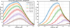 |
Fig. 10. Comparison of end-to-end performance with automatic, weighted OGCs (left), and no modal compensation (right), depending on the integrator scalar gain g, for various atmospheric r0. An MR = 0 guide star is used. Error bars show ±1 standard deviation of the frame-by-frame SR. |
The maximum SR achievable while sweeping the scalar integrator gain g is increased by the introduction of OGCs in all the situations simulated. While the improvements are modest for median seeing in the MR = 0 simulation (Fig. 10), namely 74% to 78% for r0 = 14.5 cm, the increase in SR is valuable when r0 is below 10 cm: maximal performances of 7 and 17% for r0 of 7.0 and 8.5 cm are improved to respectively 21 and 38% of H-band SR.
Significant improvements are also obtained for the high noise MR = 16 case, as seen in Fig. 11, for all seeing conditions. Overall, the use of automatic OGCs is expected to greatly increase the range of possible sky conditions for a given astronomical observation with a minimum acceptable SR, thus improving telescope availability.
Another result is conveyed that has been implicitly leveraged when describing the bootstrap sequence in Sect. 6.1. When using automatic, weighted OGCs, for each Fried parameter r0 the integrator gains gmax (r0) which yield the maximum SR are within a much narrower range than when not using OGCs. Due to the loss in sensitivity as seeing degrades, gmax (r0) continuously increases if no modal gain compensation is applied:to over 1 for r0 ≤ 8.5 cm and to over 1.5 for r0 = 7 cm. This drift is induced by the strong sensitivity loss for the low-order modes being compensated overall by increasing gmax (r0), and in itself requires manual or automatic optimization procedures if no OGCs are to be used. With the automatic, weighted OGCs on the other hand, gmax (r0) is bound between 0.45 and 0.6 for both guide stars and at all r0.
This allows us to choose a nominal integrator gain of 0.5 when using OGCs. With this constant g value set, we can budget that while the OGCs automatically update, the performance obtained is within 2% SR of the maximum achievable value when tuning g.
Finally, some selected PSF profiles corresponding to the best SRs in Fig. 10 are compared in Fig. 12. Additional speckles when comparing PSFs made without OGCs – but optimizing the global integrator gain – to those with OGCs are located mainly in two particular areas of the focal plane: the low-mid-frequencies (from 4 to 20 ), and the DM frequency limit (centered on 42–44
 ); this difference is most clearly seen on the r0 = 10.0 cm and 7.0 cm profiles. These localized degradation zones are a consequence of the impossibility to reach an optimum for all modes by only tuning the scalar integrator gain, with merely a compromise achieved. The trade-off induced at gmax when not using OGCs leads to an overshooting regime of the high-frequency modes, while mid-range modes suffer from under-compensation. At the crossing of these two regimes – for spatial frequencies of 25
 – there are modes for which the optimum rejection regime is reached, both with and without OGCs; at this location the PSFs show an identical speckle floor level.
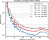 |
Fig. 12. PSF profiles corresponding to the maximum SR attained in Fig. 10, with and without using OGCs (automatic, weighted), for a turbulence r0 of 14.5, 10.0, and 7.0 cm. |
7. End-to-end simulation results – automatic gain tracking
As we look towards our design for a fully automatic OG compensation process, we have demonstrated that automatic, weighted OGCs obtained through a bootstrap sequence yield an improved AO performance in all compared seeing and guide star magnitude conditions. We now assess the long-run capacity of regular command matrix updates to maintain the AO in a near optimum state when seeing conditions need not remain stationary throughout an observation.
7.1. Variable r0 – Methods
To demonstrate the robustness of the self-updating OGC method in telescope-like conditions – in particular regardless of the seeing and without intervention of the operator during the acquisition run – we designed an end-to-end simulation protocol which covers large variations in seeing. Two simulation runs were performed: (1) where r0 gradually decreases with time from 21 to 7.0 cm over the course of 20 min and (2) the mirrored variation where r0 increases from 7.0 back to 21 cm. The performance of several AO optimization strategies is compared across these two runs.
These strategies, described hereafter, cover what is to be done with the loop gain g and the OGCs at the beginning of the experiment, and how to automatically track seeing variations. During each experiment, the AO loop is run continuously for 20 min; each minute, r0 is increased or decreased by 5.6%, and – depending on the method – the integrator gain or the OGCs are updated to track this change. A SR measurement is obtained each minute from the average of two PSFs exposed for one second each, taken immediately before and after the control law update, if any. Four methods for the initial RTC state and the update sequence are compared:
Method A: complete automatic OGC pipeline. Method A is the complete development of the automatic OG compensation process that is proposed in this research. Automatic, weighted OGCs are set through an initial bootstrap sequence at the starting r0. The integrator gain is set to 0.5 and remains unchanged. At each minute of the simulation, a single OGC update sequence is performed that lasts 1.1 s and progressively updates the modal coefficients while the r0 changes. This method, which is the product of all the analyses presented in this paper, is expected to be one of the best possible automatic strategies to go through the designed experiment with maximum performance.
Method B: initial OGCs, no update. The integrator gain is set to 0.5 and automatic, weighted OGCs at the starting r0 are set. No control updates are performed. This method simulates the impact of a one-shot modal gain optimization upon loop closing, after which the system is left unattended and unmodified across long acquisition runs. By construction, the initial state with methods A and B is identical, with an increasing difference between their performances as r0 drifts from its initial value.
Method C: initial gMax, no OGCs. The integrator gain is set to gmax (r0) for the starting r0, as obtained from the results of Sect. 6.2. No OGCs are used, and no control updates are performed. Altogether, method C is the best effort performance if restricted to manually tuning the loop gain at the beginning of an observation and not using modal OG compensation.
Method D: median OGCs, gMax updates. Reference automatic, weighted OGCs are set using the near-median r0 = 14.5 cm. These OGCs are never updated, but the integrator gain is updated every minute to the appropriate gMax (r0), as tabulated from stationary end-to-end simulations with a MR = 0 guide star. This method simulates using some fixed, median optimal gains deemed almost always adequate, and leaving the final in-situ optimization to the integrator gain. Method D was suggested and introduced as a possible technical simplification of method A.
The end-to-end performance results for the r0-varying experiments with all four methods, using MR = 0 and MR = 16 guide stars, are shown in Fig. 13.
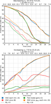 |
Fig. 13. Comparative analysis of end-to-end AO performance through an observation where (top) r0 decreases and (bottom) r0 increases between 7.0 cm and 21.0 cm – in steps of ± 5.6% every minute – depending on the method chosen for integrator gain and OGCs. Results are compiled for guide stars of magnitude 0 (solid) and 16 (dashed). Error bars of ±3% of SR are to be assumed for all data. The general simulation procedure and methods (A–D) are detailed in the main text. |
7.2. Variable r0 – Results
As expected, the automatic pipeline we propose – method A – satisfactorily maintains AO performance throughout both 20 min cycles, with identical behavior for improving or deteriorating turbulence conditions. This demonstrates that recurring OGC update sequences can satisfactorily maintain the AO in a stable and efficient state during long closed-loop runs. When comparing to the maxima for stationary r0 shown in Figs. 10 and 11, the performance is consistently inferior by 2–5% of the SR when crossing the given r0 value. When considering this loss however, the following must be taken into account: (1) the value of 0.5 not being the exact gMax (r0); and (2) the measurement by averaging the SR immediately before and after the OGC update. The choices of the variation speed of r0 and the frequency of updates are individually somewhat arbitrary, but it is demonstrated that a single update sequence can efficiently overcome r0 variations of 5.6%. We acknowledge we are missing statistics on the temporal variations of r0, but such data are beyond the scope of the present paper. Anyhow, such statistics are expected to be extremely variable depending on the moment in the year, the site, the telescope, and its dome. Altogether, we estimate that 5.6% ought to be a conservative bound for a one-minute change, and if this were found not to be the case, the frequency of OGC update sequences could easily be increased.
On the other hand, the nonupdating methods B and C show comparable performance for decreasing r0, which is as expected substantially below that of method A. When r0 deteriorates below 9.5 and 11.5 cm for magnitude 0 and 16 guide stars, respectively, the SR drops below 5%, while method A reaches this level at r0 = 9 cm for MR = 16, and maintains a SR of above 19% for MR = 0. For these methods, the decreasing and increasing r0 experiments are not equivalent. When seeing degrades, the sensitivity decreases from the initial state at r0 = 21 cm, and the system suffers an under-compensation. On the other hand, for increasing r0, the sensitivity of the PWFS continuously increases as compared to the initial state. Hence, the AO loop quickly reaches instability regimes, which in turn degrades the wavefront quality, which in turn stabilizes the loop thanks to the added residual and its inherent sensitivity reduction. This general overshoot trend accounts for the asymmetry of the two experiments for methods B and C, and is the origin of the dip in method B data for 10 ≤ r0 ≤ 14 cm. Data for methods B and C for increasing r0 past 10 cm can altogether be disregarded, as the buildup in focal plane artifacts make it undesirable to do science in such regimes. This effect is connected to the overshoot regimes which are described in Appendix A.
Besides method A, method D is the most fitting candidate for an automatic tracking of optical gain. End-to-end performances for MR = 0 are similar within SR measurement uncertainty, and for MR = 16, method D yields better performance by at most 8% SR when r0 is beyond 17 cm in the decreasing r0 sequence. This performance improvement is explained by the shape of the OGC curves used, and their relationship to S/N optimization: when taking the ratio between automatic OGCs at r0 > 14.5 cm as used by method A, and automatic OGCs at r0 = 14.5 cm, one observes that method D benefits – thanks to the trends of sensitivity measurements with seeing – from a reduction of the gain of high-order modes relative to that of low-order modes, which tends to follow the trend for optimum noise rejection (Gendron & Léna 1994) for high-noise regimes. Experimental data confirm this r0 > 14.5 or < 14.5 cm dichotomy, with the gap between methods A and D – in the decreasing r0 case – closing just as r0 reaches 14.5 cm. Noise-dependent control law optimization has not yet been implemented in method A.
These results tend to indicate that the simplification of the update process proposed by method D is attractive in terms of design, computational burden, and correction performance. As much as the authors would like to support this strategy, it is to be noted that method D, not being the core of this paper, has not been engineered in appropriate detail for this experiment, and still incurs some shortcomings. First, the update rule used assumes an immediate and precise knowledge of the current r0; this may be provided by another channel of telemetry, but this is yet to be determined. Second, the dithering-based method A has been designed, using the abacus interpolation method, to accommodate residual wavefront PSDs which may differ from the abacus computation regime, in particular when changing the importance of the various error budget components. On the other hand, maintaining a permanent OGC curve assumes conditions compliant with the ones in which it was computed; typically for method D an r0 close enough to the selected 14.5 cm. Robustness to highly varying noise conditions was demonstrated, yet the authors express reservations regarding variations of other parameters, in particular wind speed and direction; or the spatial extension of the guide object (multiple stars, planetoids, AGNs, etc). Finally, using method D also places the AO in a catastrophic failure regime if g or r0 are overestimated in low-noise cases, as occurred for unweighted OGCs and was discussed in Sect. 5.6. An analysis and discussion of this issue with method D are also included in Appendix A.
8. Discussion
8.1. Compatibility with imaging requirements
The automatic OG compensation pipeline was demonstrated to be satisfactory with an OGC update sequence of 1.1 s performed every minute. The question remains as to the impact of DM dithering on the scientific instrument, which might represent a potential restriction to the practical implementation of this technique.
Using dithering amplitudes based on in-situ noise assessment is the key feature: this ensures the dithering is always proportionate to the current image quality. We showed that clipping the amplitudes between 1.5 and 25.0 nm RMS per mode provided satisfactory performance, with 1.5 nm occasionally being reached from the S/N minimum requirement of Eq. (17) for MR = 0.
Nevertheless, we seek to quantify potential focal plane artifacts observed at the spatial frequency locations of the dithered modes – shown in Fig. 7 – and SR performance losses, if any. We measured the SR for cases with r0 of 14.5 and 8.5 cm and guide star magnitudes MR = 0 and 16. During an AO run lasting 20 min, the PSF was acquired during all of the 20 dithering sequences, each 0.5 s long. From these, a ten-second exposure equivalent PSF was obtained, and identically a nondithered PSF was compiled after acquiring 20 exposures of 0.5 s each immediately after dithering sequences. Measured short exposure and overall ten-second SRs are compiled in Table 3, along with the mean dithering amplitudes for the three ψi modes across the 20 ditherings performed to reach the total ten-second exposure.
H-band SR measurements during and in-between dithering sequences for various r0 and guide stars, along with mean dithering amplitudes.
Data in Table 3 show that any science channel disturbance is beyond SR measurement sensitivity. Long- and short-exposure SRs are identical within and outside of ditherings, with nearly identical temporal error bars of the short-exposure SR. Moreover, quantitative values amount to approximate maximal dithered wavefronts of 6 and 26 nm RMS adding the three modes, for MR = 0 and MR = 16, respectively.
Of the cases measured, only for r0 = 14.5 cm at MR = 16 were we capable of clearly observing dithering-induced structures in the PSF. The relative difference between dithering and nondithering PSFs is shown in Fig. 14, computed as:  .
.
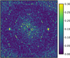 |
Fig. 14. Relative PSF difference between dithering-only and nondithering acquisitions, for r0 = 14.5 cm and MR = 16. The image is 100 |

The most prominent structure in Fig. 14 are the two side lobes on the horizontal axis, induced by mode ψ2; they may be observed on the dithered PSF, with peak magnitude of 0.06% of the PSF core. These two lobes are complemented by a near-complete ring of speckles from ψ1 and a partial hexagon of the spatial frequencies of ψ3. Speckles with higher values within the ψ1 ring are due to speckle noise between the subtracted PSFs.
Overall, our experiments indicate that the worst case disturbances induced by dithering on the science channel would only matter if contrasts better than 104 could be obtained. While this is generally not the case with the system studied, it may be for an AO followed by a coronagraphic second-stage extreme AO system. The authors suggest two possible operating modes to ensure profitable cooperation between an automatically dithering RTC and the science channel depending on the scientific acquisition mode. If long-exposure science images are being run, for example above 10 s of exposure time, a half-second dithering would be diluted across the exposure, and the AO would proceed without interrupting the science instrument; if short-exposure shots are being taken, we suggest that the instrument-control software would periodically suspend the scientific acquisitions while the dithering is performed. In such a case, dithering amplitudes can even be increased and the dithering duration shortened, together preventing a fratricide effect, with the shortest possible interruptions.
8.2. Compensating noncommon path aberrations
Early in this paper, we mentioned the critical issue of the effect of OG regarding NCPA subtraction in the AO loop. We unfortunately could not tackle this topic extensively at the time of writing this paper, and no end-to-end simulations with NCPAs had yet been performed using the dithering method. NCPA compensation was actually one of the starting points of OG analysis and gain tracking methods for high-order AO systems with nonlinear WFSs (Esposito et al. 2015). Modal OG compensation works towards the solution: considering the NCPA measurement not as reference slopes, a practice inherited from Shack–Hartmann formalism and yet unsuitable for nonlinear systems, but rather in terms of reference wavefront maps. In practice, this means performing the setpoint subtraction not as

but after the MVM computation, as

With this new point of view, an appropriate NCPA compensation can be performed adequately, leveraging the rectification of the reconstructor, and avoiding the issue of NCPA over-compensation (Bond et al. 2017) which occurs when an increase in gain is applied over Eq. (19) to compensate for sensitivity reduction.
The NCPA subtraction following Eq. (20) is appropriate regardless of whether ϕNCPA is calibrated directly as a wavefront (e.g., with phase diversity), or using the traditional method – setting the cleanest possible PSF on the imaging channel and acquiring the WFS slopes for such a wavefront, in which case it is estimated by

The latter case allows for a finer all-in-one estimation of second-order effects such as aliasing or nonlinearity of the measurement of the NCPA wavefront.
The nonlinearity induced by the NCPA offset is also to be considered for OG compensation in its own regard. Regarding the MICADO SCAO system, a total of 120–150 nm RMS residual NCPA is expected after optical precompensation during instrument commissioning. This residual NCPA alone modifies the PWFS response. For the dithering method to be applicable, we therefore expect that abacuses should be recomputed once NCPAs are fully characterized, with p0-class wavefronts offset by the ϕNCPA.
8.3. Alternative calibration and sensitivity-compensation methods
To conclude this section, we would like to discuss how the dithering and OG compensation approach presented in this paper should compare to current alternatives used to operate PWFSs on-sky. In particular, on-sky measurements of interaction matrices can be performed (Esposito et al. 2010; Guyon et al. 2011), or alternatively, adequate synthetic matrices to match on-sky sensitivity (Héritier et al. 2018).
First, we assume an on-sky interaction matrix can be measured that is appropriate to the ongoing average turbulent conditions, that is, the mean dPyr for some residual wavefront PSD. Using the associated reconstructor would then account for both the sensitivity reduction, as characterized by α∥, and the mean nonlinear modal crosstalk, quantified by d⊥ as per the definitions in Sect. 2.3. It is however possible to derive – from data obtained during the computation of the abacuses shown in Figs. 3 and 4 – that d⊥ is mainly borne by stochastic fluctuations with the wavefront realization ϕRes. Due to this property, the compensation of the mean d⊥ component for a given p0-PSD class, as could be expected with obtaining an on-sky interaction matrix, makes little to no difference as compared to the sole compensation of the colinear nonlinearity α∥ as proposed in this paper.
Furthermore, the main criterion to be considered is the actual capacity to obtain a nearly noiseless and well-conditioned on-sky interaction matrix, in particular at the ELT scale where matrices reach sizes beyond 4000 × 20 000, with the acquisition being all the more difficult on faint guide stars and in sub-median seeing conditions. For such reasons, a modal rescaling to be applied on synthetic interaction matrices is at this stage expected to be the most robust approach.
Lastly, it is sometimes suggested that a modal gain function can be directly extrapolated from sensitivity-reduction measurements, such as the ones obtained from demodulating dithered signal. In such a case, a piecewise-constant or linear curve is extrapolated, which provides gain values across the modal basis. We believe this method is numerically efficient and very comparable to our approach, and our analysis of the sensitivity as shown in Fig. 3 should provide input on how to group modes for interpolation. However, it is still the case that coefficients comparable to α∥ have to be measured for a few modes, in which case the use of a true, realistic abacus, as demonstrated here, is merely a small extra effort that enables all the features of the used DM basis to be encompassed.
9. Conclusion
In this work, the authors propose a thorough analysis of the optical gain phenomenon with the PWFS, OG being defined as a modification of the first-order response of the sensors between the calibration regime – with a flat wavefront, and operational regimes when the PWFS is shown a closed-loop residual wavefront.
We proposed a numerical approach for obtaining the gain for each mode that minimizes the first-order nonlinearity error component for a given wavefront. Through extensive numerical simulations we confirmed the hypothesis that OGCs only weakly depend (< 3%) on the wavefront, but only on its PSD, a key point to ensure the time-persistent validity of a set of OGCs. Moreover, our analysis of the residual error after modal compensation showed that low-order modes see their nonlinearity error budget greatly reduced.
There are strong variations of the OGCs when r0 varies, and a sufficiently precise telemetry would be require the appropriate modal gains to be obtained. We implemented a telescope-ready method to obtain the optimal modal gains without prior knowledge of the atmospheric conditions. Using an offline-computed database comprising sensitivity reduction and optimal gains for a variety of r0, we interpolate the optimal gain for all modes, using information acquired from the feedback of the dithering of only three DM modes over 0.5 s. The dithering-sequence mode choices, signal frequencies, and duration were engineered to provide meaningful, robust, and consistent results using the ELT AO setup on which we performed all the validating numerical simulations.
Using automatic OGCs, besides providing a method valid for a broad range of observation conditions without any operator intervention or system fine-tuning, was shown to provide valuable increases in end-to-end performances in all the configurations tested, mainly for sub-median seeings and near the limiting magnitude of the instrument. These performances are expected to provide a valuable increase both in imaging quality and in useful telescope time, by pushing the lower limit of acceptable sky conditions for scientific observations.
Furthermore, we demonstrated, through end-to-end simulations with a fast, broad-range dynamically varying r0, that the repetition of the OGC update sequence lasting 1.1 s every minute was sufficient to maintain the control law in near optimum state, without ever opening and re-closing the AO loop, even after minutes spent at r0 < 8 cm. We also investigated an alternative simplification of the method, which would optimize only the integrator scalar gain while maintaining a predefined modal gain curve. While this simplified process provided results comparable to our complete OGC automatic method, interrogations remain at this step on how to engineer a complete automatic pipeline following this altogether promising philosophy and avoiding the instability issue associated with low-order modes.
We propose a robust automatic control law protocol, tailored for telescope operation conditions, which relieves the burden of monitoring and adjusting the AO manually, with little to no effect on the operation of the scientific instrument. We strongly support the implementation of such a method or its future derivatives in ELT AO controllers, which will hopefully be a valuable asset in monitoring and optimizing AO loop internals without increased operator supervision.
Acknowledgments
This research is performed in the frame of the development of MICADO, the first light instrument of the ELT (ESO), with the support of ESO, INSU/CNRS and Observatoire de Paris. The authors also thank the members of the AO community who manifested their interest in an optical gain compensation method adjusting the integrator gain only over a nonchanging modal coefficient curve.
References
- Biasi, R., Manetti, M., Andrighettoni, M., et al. 2016, Proc. SPIE, 9909, 99097Y [NASA ADS] [CrossRef] [Google Scholar]
- Bond, C. Z., Correia, C. M., Sauvage, J. -F., et al. 2017, in 5th AO4ELT Conference-Adaptive Optics for Extremely Large Telescopes [Google Scholar]
- Clénet, Y., Buey, T., Gendron, E., et al. 2018, Proc. SPIE, 10703, 1070313 [Google Scholar]
- Clergeon, C. 2014, Ph. D. Thesis, Observatoire de Paris – Subaru National Astronomical Observatory of Japan [Google Scholar]
- Deo, V., Gendron, E., Rousset, G., et al. 2018a, Proc. SPIE, 10703, 1070320 [Google Scholar]
- Deo, V., Gendron, E., Rousset, G., et al. 2018b, A&A, 619, A56 [NASA ADS] [CrossRef] [EDP Sciences] [Google Scholar]
- Esposito, S., & Riccardi, A. 2001, A&A, 369, L9 [NASA ADS] [CrossRef] [EDP Sciences] [Google Scholar]
- Esposito, S., Tubbs, R., Puglisi, A., et al. 2006, Proc. SPIE, 6272, 62721C [NASA ADS] [CrossRef] [Google Scholar]
- Esposito, S., Riccardi, A., Fini, L., et al. 2010, Proc. SPIE, 7736, 773609 [CrossRef] [Google Scholar]
- Esposito, S., Pinna, E., Puglisi, A., et al. 2015, in 4th AO4ELT Conference-Adaptive Optics for Extremely Large Telescopes [Google Scholar]
- Fauvarque, O., Neichel, B., Fusco, T., Sauvage, J.-F., & Girault, O. 2016, Optica, 3, 1440 [NASA ADS] [CrossRef] [Google Scholar]
- Fauvarque, O., Janin-Potiron, P., Correia, C., et al. 2019, JOSA A, 36, 1241 [Google Scholar]
- Ferreira, F., Gratadour, D., Sevin, A., et al. 2018a, Proc. SPIE, 10703, 1070347 [Google Scholar]
- Ferreira, F., Gendron, E., Rousset, G., & Gratadour, D. 2018b, A&A, 616, A102 [NASA ADS] [CrossRef] [EDP Sciences] [Google Scholar]
- Frazin, R. A. 2018, JOSA A, 35, 594 [NASA ADS] [CrossRef] [Google Scholar]
- Gendron, E., & Léna, P. 1994, A&A, 291, 337 [NASA ADS] [Google Scholar]
- Guyon, O., Martinache, F., Clergeon, C., et al. 2011, Proc. SPIE, 8149, 814908 [NASA ADS] [CrossRef] [Google Scholar]
- Héritier, C. T., Esposito, S., Fusco, T., et al. 2018, Proc. SPIE, 10703, 107034P [Google Scholar]
- Hutterer, V., & Ramlau, R. 2018, Appl. Opt., 57, 8790 [NASA ADS] [CrossRef] [Google Scholar]
- Kolb, J., Madec, P. Y., Le Louarn, M., Muller, N., & Béchet, C. 2012, Proc. SPIE, 8447, 84472D [NASA ADS] [CrossRef] [Google Scholar]
- Korkiakoski, V., Vérinaud, C., & Le Louarn, M. 2008a, Proc. SPIE, 7015, 701554 [CrossRef] [Google Scholar]
- Korkiakoski, V., Vérinaud, C., & Le Louarn, M. 2008b, Appl. Opt., 47, 79 [NASA ADS] [CrossRef] [Google Scholar]
- Neichel, B., Fusco, T., & Sauvage, J. F., et al. 2018, Proc. SPIE, 10703, 1070322 [Google Scholar]
- Pinna, E., Agapito, G., Quirós-Pacheco, F., et al. 2014, Proc. SPIE, 9148, 914804 [CrossRef] [Google Scholar]
- Ragazzoni, R. 1996, J. Mod. Opt., 43, 289 [NASA ADS] [CrossRef] [Google Scholar]
- Ragazzoni, R., & Farinato, J. 1999, A&A, 350, L23 [Google Scholar]
- Rigaut, F., Neichel, B., Bec, M., et al. 2010, in 1st AO4ELT Conference-Adaptive Optics for Extremely Large Telescopes, EDP Sciences [Google Scholar]
- Sedghi, B., Muller, M., Bonnet, H., Dimmler, M., & Bauvir, B. 2010, Proc. SPIE, 7733, 773340 [NASA ADS] [CrossRef] [Google Scholar]
- Shatokhina, I. 2014, Ph. D. Thesis, Johannes Kepler Universität Linz, Austria [Google Scholar]
- Véran, J. P., Esposito, S., Spanò, P., Herriot, G., & Andersen, D. 2016, in 4th AO4ELT Conference-Adaptive Optics for Extremely Large Telescopes [Google Scholar]
- Vérinaud, C. 2004, Opt. Commun., 233, 27 [NASA ADS] [CrossRef] [Google Scholar]
- Vidal, F., Ferreira, F., Deo, V., et al. 2017, in 5th AO4ELT Conference-Adaptive Optics for Extremely Large Telescopes [Google Scholar]
- Viotto, V., Bergomi, M., Dima, M., et al. 2016, Proc. SPIE, 9909, 99096H [Google Scholar]
Appendix A: Stability issues and OGC weighting
For some modal gain coefficient curves, a catastrophic failure of the AO loop may happen for small increases of the loop gain or the PWFS sensitivity. This effect is discussed in the main text in Sect. 5.6, and was the motivation for our introduction of a weighting of the OGCs defined by Eq. (18).
This appendix documents and discusses how this instability phenomenon is manifested with some OGC computation techniques, when a sensitivity increase – due to the integrator gain, or an increase in r0 – sets the lowest-order modes of the DM into oscillatory regimes. We recall that very low-order modes – mainly tip-tilt – bear the most turbulence residuals, are most affected by OG, and therefore most compensated, and suffer the least reconstruction error when appropriately compensated, as was discussed in Sect. 4.2. Frame-to-frame oscillations of these modes are destructive for the imaging quality, with a PSF core either bearing strong artifacts or tracing patterns in long-exposure images due to a wandering tip-tilt.
We performed identical experiments to those used to demonstrate the performance of automatic, weighted OGCs for a given r0 (Figs. 10 and 11), comparing the long exposure SR with the varying integrator gain g. Here, we study three OGC methods: (1) unweighted, automatic OGCs; (2) the sensitivity compensation coefficients (SCC) proposed in Korkiakoski et al. (2008b), defined as
with the norms taken in the PWFS slope space; and (3) automatic, weighted OGCs measured at r0 = 14.5 cm and then unchanged, as used in method D of Sect. 7. Results for these three possible OGC computations are shown in Fig. A.1, using a MR = 0 guide star, and exhibit the infamous gap effect in the SR(g) data at the higher r0 values. With the global variation of sensitivity with r0, dynamic variations in r0 – or misestimations thereof – not accounted for by automatic OGC updates are equivalent to a left-shift or a right-shift of the SR(g) curves as r0 increases or decreases, respectively. With g set to gMax (r0), a sudden r0 increase therefore results in the SR collapsing as tip-tilt becomes unstable.
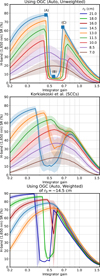 |
Fig. A.1. End-to-end performance measurements for various OG modal-compensation techniques, probing for maximum SR depending on integrator gain g at various stationary r0 from 7.0 to 21 cm, using a MR = 0 guide star. Top: unweighted automatic OGCs; middle: SCCs as per Korkiakoski et al. (2008b); bottom: using automatic, weighted OGCs computed at r0 = 14.5 cm and reused identically at all r0, as per method D of Sect. 7.1. Labeled markers on top graph: PSFs are shown in Figs. A.2a–A.2c. |
For unweighted, automatic OGCs, the gap effect means an immediate degradation of the SR to below 10% with sensitivity increases, observed for all r0 ≥ 8.5 cm. Similarly, the OGCs taken for r0 = 14.5 cm and unchanged exhibit a gap for r0 > 14.5 cm. This effect was not observed in the dynamically increasing r0 experiments shown in Sect. 7.2, yet only because the tabulated gmax were taken, conservatively, to be smaller than the gap edge, hence ensuring the r0 increases of 5.6% each minute were tolerated by method D.
For the SCCs, it is interesting to note they also exhibit the gap behavior for r0 ≥ 11.5 cm, although less markedly. We suggest that this is linked to the computation method, performed in the higher-dimensionality slope space rather than modal space; this yields OGC curves spanning a larger range across the modal basis. Hence, for an identical gain of the low-order modes, highest-frequency modes bear a higher gain than for automatic OGCs, and in turn provide the self-stabilizing increase in wavefront residual slightly sooner than our Gopt coefficients.
We wish to mention that similar effects could not be reproduced for these SCCs on an 18 m simulated telescope (Deo et al. 2018a), and therefore that the gap effect is thought to be strongly correlated with the ever-increasing dimensionality – and complexity – of the AO system with telescope size.
How the gap effect impacts the tip-tilt and its successful compensation with OGC weighting is best seen using PSFs corresponding to various g values during the experiments. Figures A.2a–A.2c show PSFs taken across the gap for automatic, unweighted OGCs at r0 = 14.5 cm, corresponding to points labeled (A)–(C) in Fig. A.1 (top). At a gain of 0.60 – in combination with gmax = 0.46 – the PSF is completely blurred by tip-tilt oscillations, which smear the core into an elliptic pattern a few  across. Reaching past this regime at g = 0.68, waffle modes enter oscillatory regimes, with corresponding artifacts at the corners of the DM rejection domain, and in turn tip-tilt sensing is sufficiently dampened to induce a stabilized PSF core and restore a decent SR over 60%.
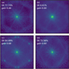 |
Fig. A.2. Analysis of the PSF structure during the SR gap effect when continuously increasing the integrator gain. (a)–(c): PSFs from unweighted OGC runs, corresponding to points labeled (A)–(C) in Fig. A.1 (top). (d): PSF taken with parameters equivalent to those in (b) but with weighted OGC, corresponding to Fig. 10. All PSFs are shown in log scale, with colormaps spanning from 3.10−6 to 1, where 1 is a 100% SR PSF. |
The PSF in Fig. A.2d is taken with all identical parameters to those in Fig. A.2b except for the added weighting. This PSF demonstrates how the image is satisfactorily stabilized, and the mid-frequency range speckle halos engineered by Eq. (18) and synthetically imaged in Fig. 9 are clearly noticeable. While this regime is not meant to be reached and provides a PSF with some artifacts, it is only transitory with sudden improvements of the seeing until the following OGC update sequence; weighting satisfactorily prevents the catastrophic failures of the other OGC computation techniques presented.
All Tables
H-band SR measurements during and in-between dithering sequences for various r0 and guide stars, along with mean dithering amplitudes.
All Figures
|
Fig. 1. Top: PWFS slopes vector for a flat wavefront, a 300 nm RMS tilt, and the same tilt added to a 120 nm RMS fitting error wavefront ϕRes, showing the attenuation of the signal. Data are smoothed by a window of 50 samples in width for clarity. Bottom: recorded PWFS response curve to three modes – tilt and Karhunen–Loève 20 and 3000 – with and without the same ϕRes. The tilt curve without residuals saturates around 750 nm RMS. The AO setup simulated is described in Sect. 3. |
| In the text | |
|
Fig. 2. Schematic OG-impeded reconstruction of a mirror mode |
| In the text | |
|
Fig. 3. Subset of the α∥ abacus data. Solid lines: μ[α∥ (ϕi;p0)]; shaded areas: ±2σ[α∥ (ϕi;p0)], as computed numerically on 15 independent wavefronts of class p0 in conditions of Table 1, except that no noise is introduced. Curves are smoothed for improved clarity using an adaptive recursive filter with window width log (i). |
| In the text | |
|
Fig. 4. Subset of the Gopt abacus data. Solid lines: μ[Gopt (ϕi;p0)]; shaded areas: ±2σ[Gopt (ϕi;p0)]. Data computed and smoothed as in Fig. 3. |
| In the text | |
|
Fig. 5. Error terms with and without applying static Gopt (ϕi; p0) OGCs. Solid lines: μ[||eOpt (p0)||] (with OGCs); dashed lines: μ[||eRec (p0)||] (without modal compensation); shaded areas: ±2 standard deviations. Data computed and smoothed as in Fig. 3. |
| In the text | |
|
Fig. 6. Typical example of a dithering sequence, as we use for all numerical simulations using the dithering method in this paper. “DM dithering”: ψi amplitude injected Ai × ||ψi|| × cos (2πfit); “Mode ampl. on PWFS”: true instantaneous component in ψi of the wavefront; “PWFS reconstruction”: ψi component measured from the slopes, i.e., ||ψi||−2 × ψi ⊗ (Rec⋅S (t)). For this case, the turbulence r0 is 14.5 cm, with conditions of Table 1 but no noise. Wavefront maps of the ψi are shown in Fig. 7. Data for ψ1 and ψ3 are offset by +20 and −20 nm, respectively. |
| In the text | |
|
Fig. 7. Wavefront maps (left column) and log-scaled spatial PSD (right) for the dithered modes ψ1, 2, 3. The displayed area is 39.5 m across for wavefront maps and |
| In the text | |
|
Fig. 8. Successive steps of the abacus-based interpolation process. (a) For each of the K dithered modes ψi, the measurement |
| In the text | |
|
Fig. 9. Top: corrective OGC weighting W(i), as defined per Eq. (18), for the ELT simulation with N = 4309 modes. Bottom: distribution of the weighting W(i) in the Fourier plane of the pupil. At each frequency in the Fourier plane, the weight shown is the W(i) of the KL mode which bears the most energy at that specific frequency. This representation is obtained by computing the Fourier transform of all modes and finding the mode that is most representative of any given spatial frequency. The dashed hexagon shows the correction zone of the M4 DM. The displayed area is 100 |
| In the text | |
|
Fig. 10. Comparison of end-to-end performance with automatic, weighted OGCs (left), and no modal compensation (right), depending on the integrator scalar gain g, for various atmospheric r0. An MR = 0 guide star is used. Error bars show ±1 standard deviation of the frame-by-frame SR. |
| In the text | |
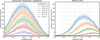 |
Fig. 11. Identical to Fig. 10, using a MR = 16 guide star. |
| In the text | |
|
Fig. 12. PSF profiles corresponding to the maximum SR attained in Fig. 10, with and without using OGCs (automatic, weighted), for a turbulence r0 of 14.5, 10.0, and 7.0 cm. |
| In the text | |
|
Fig. 13. Comparative analysis of end-to-end AO performance through an observation where (top) r0 decreases and (bottom) r0 increases between 7.0 cm and 21.0 cm – in steps of ± 5.6% every minute – depending on the method chosen for integrator gain and OGCs. Results are compiled for guide stars of magnitude 0 (solid) and 16 (dashed). Error bars of ±3% of SR are to be assumed for all data. The general simulation procedure and methods (A–D) are detailed in the main text. |
| In the text | |
|
Fig. 14. Relative PSF difference between dithering-only and nondithering acquisitions, for r0 = 14.5 cm and MR = 16. The image is 100 |
| In the text | |
|
Fig. A.1. End-to-end performance measurements for various OG modal-compensation techniques, probing for maximum SR depending on integrator gain g at various stationary r0 from 7.0 to 21 cm, using a MR = 0 guide star. Top: unweighted automatic OGCs; middle: SCCs as per Korkiakoski et al. (2008b); bottom: using automatic, weighted OGCs computed at r0 = 14.5 cm and reused identically at all r0, as per method D of Sect. 7.1. Labeled markers on top graph: PSFs are shown in Figs. A.2a–A.2c. |
| In the text | |
|
Fig. A.2. Analysis of the PSF structure during the SR gap effect when continuously increasing the integrator gain. (a)–(c): PSFs from unweighted OGC runs, corresponding to points labeled (A)–(C) in Fig. A.1 (top). (d): PSF taken with parameters equivalent to those in (b) but with weighted OGC, corresponding to Fig. 10. All PSFs are shown in log scale, with colormaps spanning from 3.10−6 to 1, where 1 is a 100% SR PSF. |
| In the text | |
Current usage metrics show cumulative count of Article Views (full-text article views including HTML views, PDF and ePub downloads, according to the available data) and Abstracts Views on Vision4Press platform.
Data correspond to usage on the plateform after 2015. The current usage metrics is available 48-96 hours after online publication and is updated daily on week days.
Initial download of the metrics may take a while.