| Issue |
A&A
Volume 687, July 2024
|
|
|---|---|---|
| Article Number | A198 | |
| Number of page(s) | 17 | |
| Section | Astronomical instrumentation | |
| DOI | https://doi.org/10.1051/0004-6361/202449254 | |
| Published online | 12 July 2024 | |
Multi-purpose InSTRument for Astronomy at Low-resolution: MISTRAL at the Observatoire de Haute-Provence
1
OHP, OSU – Institut Pythéas, UAR 3470, CNRS, Aix-Marseille Université,
1912 Route de l’Observatoire,
04870
St.Michel l’Observatoire, France
e-mail: This email address is being protected from spambots. You need JavaScript enabled to view it.
2
Aix Marseille Univ, CNRS, CNES, LAM,
Marseille, France
3
Sorbonne Université, CNRS, UMR 7095, Institut d’Astrophysique de Paris,
98bis Bd Arago,
75014
Paris, France
4
OSU – Institut Pythéas, UAR 3470, CNRS, Aix-Marseille Université, Pôle de l’Étoile Site de Château-Gombert,
38 rue Frédéric Joliot-Curie
13388
Marseille, France
5
Physical Research Laboratory,
Navarangpura,
Ahmedabad,
380058
Gujarat, India
6
Space sciences, Technologies & Astrophysics Research (STAR) Institute,
Allée du Six Août, 19C, University of Liège,
4000
Liège, Belgium
7
CEA, IRFU, DAp, AIM, Université Paris-Saclay, Université Paris Cité, Sorbonne Paris Cité, CNRS,
91191
Gif-sur-Yvette, France
8
GEPI, Observatoire de Paris, Université PSL, CNRS,
5 Place Jules Janssen,
92190
Meudon, France
9
Kavli Institute for Astrophysics and Space Research, Massachusetts Institute of Technology,
Cambridge, MA, USA
10
IRFU, CEA, Université Paris-Saclay,
Gif-sur-Yvette, France
Received:
17
January
2024
Accepted:
3
April
2024
Abstract
Context. Multi-purpose InSTRument for Astronomy at Low-resolution (MISTRAL) is the new Faint Object Spectroscopic Camera mounted at the folded Cassegrain focus of the 1.93 m telescope of the Haute-Provence Observatory (OHP).
Aims. We describe the design and components of the instrument and give some details about its operation.
Methods. We emphasize in particular the various observing modes and the performance of the detector. A short description of the working environment is also provided. Various types of objects, including stars, nebulae, comets, novae, and galaxies, have been observed during various test phases to evaluate the performance of the instrument.
Results. The instrument covers the range of 4000-8000 Å with the blue setting, or from 6000 to 10 000 Å with the red setting, at an average spectral resolution of 700. Its peak efficiency is about 22% at 6000 Å. In spectroscopy, a limiting magnitude of r ~ 19.5 can be achieved for a point source in one hour with a signal-to-noise ratio of 3 in the continuum (and better when emission lines are present). In imaging mode, limiting magnitudes of 20–21 can be obtained in 10–20 mn (with average seeing conditions of 2.5 arcsec at the OHP). The instrument is very user-friendly and can be put into operations in less than 15 mn (rapid change-over from the other instrument in use) if required by the science (e.g. for gamma-ray bursts). Some first scientific results are described for various types of objects, and in particular, for the follow-up of gamma-ray bursts.
Conclusions. While some further improvements are still under way, in particular, to facilitate the switch from blue to red setting and add more grisms or filters, MISTRAL is ready for the follow-up of transients and other variable objects, in the soon-to-come era of the Space-based multi-band astronomical Variable Objects Monitor satellite and of the Rubin telescope, for instance.
Key words: instrumentation: photometers / instrumentation: spectrographs
Based on observations obtained with Observatoire de Haute-Provence (OHP) instruments (see acknowledgements for more details).
© The Authors 2024
 Open Access article, published by EDP Sciences, under the terms of the Creative Commons Attribution License (https://creativecommons.org/licenses/by/4.0), which permits unrestricted use, distribution, and reproduction in any medium, provided the original work is properly cited.
This article is published in open access under the Subscribe to Open model. This email address is being protected from spambots. You need JavaScript enabled to view it. to support open access publication.
1 Introduction
With the advent of many new sky surveys starting in 2010 from the ground and from space, the exploration of the variable sky has become a highly competitive new domain of Astrophysics (e.g. Graham et al. 2019, and references therein). The high cadence of these surveys in the framework of multi-messenger astrophysics and the large area they cover led to the discovery of a wealth of new phenomena and classes of objects, enlarging the observed physical diversity and improving the statistics on previously known types of objects. This will still increase in the near future, with the advent of the Vera C. Rubin Telescope and the launch of SVOM, and it will require a major effort of ground-based follow-up. At high energy, gamma-ray bursts (GRBs; e.g., Gehrels et al. 2009) are observed in large numbers and are classi fied into two categories, the short- and long-duration GRBs. The early classification of supernovae (SNe; e.g., Gal-Yam 2017) into types I or II apparently needs to be refined, however, to take the variety of observed phenomena into account: we know not just core-collapse or thermonuclear explosions of CO white dwarfs, but also ultraluminous SNe or faint and fast-decaying type I SNe, He detonation Ia objects, or objects that interact with the circum-stellar medium (CSM), and there is also the variety of novae. The range of underlying physical mechanisms is therefore much more diverse than previously thought, but it is still not understood. Luminous blue variables, or the numerous peculiar binaries, also await a better understanding.
Nontransient but variable objects also require some follow-up. For instance, it was found that some quasars show dramatic changes in luminosity and spectral characteristics. These are the so-called changing-look quasars (e.g., MacLeod et al. 2016 and references therein), whose changes are not compatible with the standard model of active galactic nuclei (AGN). Increas ingly more objects are found of this type, and they require more long-term monitoring to measure timescales and possible delays between the changes in the optical and other wavelengths.
On the other hand, large spectroscopic catalogs (e.g., the Sloan Digital Sky Survey: SDSS1) are rarely 100% complete or do not always cover the high-latitude regions (see, e.g., the XMM Cluster Archive Super Survey: XCLASS; Koulouridis et al. 2021). Moreover, the spectra available in the literature are sometimes of poor quality because they were taken to obtain a redshift or a general classification of the objects, and the signal-to-noise ratio is insufficient to detect faint characteristic lines, or the spectral coverage is too short to explore the red part of the spectrum, for instance. Enough ground-based observing time is most needed for progress in all these fields to follow the evo lution of representative examples of all those categories over time. Photometry, and even more, spectroscopy is required that includes the near-infrared, if possible: only with long time-series of data is it possible to understand the underlying physical mech anisms. Small to medium telescopes are now more available for long time-series than the 8 m telescopes, and they are well suited for this task if they are equipped with efficient versatile spectro-imagers. The Observatoire de Haute Provence has pioneered in the early exploration of the far-red range (6000–11000 Å), first with the Roucass spectrograph (Andrillat et al. 1975), and later with the Carelec spectrograph (Lemaitre et al. 1990). Since the decommissioning of the latter in 2012, no low-dispersion spec-troscopic facility was available any longer, at a moment where it is much needed again.
It is with this in mind that the MISTRAL2 instrument had been planned for the OHP 1.93 m telescope, with a possibility of rapid reaction (targets of opportunity: ToO) and changeover from the other OHP T193 instrument, SOPHIE. While the con cept of the focal reducer was invented long ago by G. Courtes in Marseille (Courtes 1960), no such instrument was permanently installed at the OHP. With the development of transient astron omy, a flexible instrument like this became mandatory and was envisaged already for the launch of Gaia alerts. Various issues delayed the project (see below), but the gap is now filled, and the MISTRAL instrument entered into service in 2021.
MISTRAL can be operated in two modes: regular observing runs in visitor mode, and target of opportunity mode with ser vice observing for fast transients. MISTRAL can be accessed by any astronomer working in a French astronomical institution via the national call for observing proposals, which uses the North-Star3 system. Non-French nationals can also access it through the Transnational Access Program of the Opticon RadioNet Pilot program4, which includes a wide range of worldwide institutions5.
In the next section, we describe the main components of MISTRAL and give some details on the operation mode and tools available for the observer. As on-sky instrument per formance validations, we present in Sect. 3 real observations demonstrating the ability of MISTRAL to access faint objects of various types, including access to near-infrared lines (e.g., the Paschen lines), and to spectroscopically classify them. To assess the ability of MISTRAL to obtain spectra with a higher spectral resolution, we also investigate the spectral resolution of MIS TRAL around Hα. This section finally shows that we can follow moving targets with a report of a comet follow-up. Section 4 describes the core of the MISTRAL activities: GRB follow-ups. We detail several observations with an intrinsic scientific interest (e.g., the Brightest Of All Time GRB: BOAT hereafter). Finally, more details about the instrument operations are given in the appendices.
2 General description of the instrument
2.1 General setup
A versatile spectro-imager should cover a wavelength range that is as large as possible to cover the various science goals described above. This ideal is limited by the size of the detector, which is here a single detector with 2048 pixels. While the ini tial idea was then to follow the path of SPRAT (SPectrograph for the Rapid Acquisition of Transients) at the Liverpool telescope (Piascik 2017) to speed up the development, it rapidly became clear that several factors prevented this simple approach. First of all, the 1.93 m telescope being a relatively old telescope, its f/ratio at Cassegrain focus is f/15, in contrast to more modern telescopes, which are at f/10 or faster: to avoid an instrument that was too long, a focal reducer had thus to be introduced. Second, since the decommissioning of the Carelec, the main instrument at the 1.93 m was a high-resolution spectrograph for exoplanet research with the velocimetry technique (SOPHIE), requiring a good long-term stability. Rapid change-overs needed for ToO observations were therefore not compatible with this require ment. The ideal solution would have been a common adapter for both instruments (SOPHIE is fed by fibers), but this could not be implemented in time. It was therefore decided to mount MIS TRAL at the folded Cassegrain focus, and the change-over from one instrument to the next was simply effected by placing and removing a flat 45° mirror in the main beam: the change-over is done this way in less than 15 min (including adjustment of the telescope focus). Because the mechanical design with respect to SPRAT had to be changed regardless, we took advantage of these changes to implement more flexibility in the instrument, such as introducing a filter holder and a grism holder, where different components can be introduced in the parallel beam by simply moving (sliding) these holders: the exchange is done in a few seconds. The large OHP telescopes are operated with a telescope operator on site, and this therefore slightly relaxed the constraints on mechanical and pointing accuracy because the acquisition and centering into the slit is always checked visually.
The mechanical design includes a motorized 45° flat mirror within the T193 Cassegrain adapter, which needs to be moved in the beam to redirect the light onto MISTRAL (at the folded Cassegrain focus) or has to be moved out of the beam for the other instrument, SOPHIE, which is fed at the direct Cassegrain focus. MISTRAL is mounted on one of the side slots of the T193 adapter. The other adapter opposite this adapter is still empty. Figure 1 shows the instrument. The focusing on the slit is made by moving the secondary mirror of the telescope, and the focusing on the detector is made by moving the detector holder. A guiding camera is directly associated with the instrument to minimize mechanical flexures6.
These modifications nevertheless led to a relatively simple instrument with a long-term stability (see Appendix F) as it is permanently mounted to the telescope and very easy to operate for first-time users.
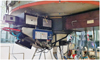 |
Fig. 1 MISTRAL (to the left of the image) installed at the folded Cassegrain focus of the 1.93 m telescope at OHP. |
2.2 Optical path and detector
MISTRAL is mounted at the folded-Cassegrain focus of the 1.93 m telescope via a focal reducer. This focal reducer reduces the beam from F/15 to F/6 at the entrance slit. At the exit on the detector, the opening is F/3. The entrance slit is currently fixed at a width of 112 microns, translating into 1.9″ on the sky, but a variable slit is under construction (the average seeing at OHP is around 2″). At the end, the beam falls on an ANDOR deep-depletion 2K×2K CCD camera (iKon-L DZ936N BEX2DD CCD-22031) with 13.5 µ pixels, giving therefore slightly more than 4 pixels per slit width on the detector. This allows for some smoothing in the spectra to increase the signal-to-noise ratio, if needed. The cooling is made by a five-layer Peltier device. The operating temperature is −90C to −95C. The dark current is lower than 3 electrons/hour/pixel. The sliding plate holding the gratings currently has two grisms, for the blue (roughly 4000 8000 Å) or the red (6000–10 000 Å) range, but two more slots are available. The spectral resolution is about 700 at 6000 Å (see Appendix C for more details). The FLI filter wheel has 12 posi tions for 50 mm filters (currently available are SDSS ɡ′, r′, i′, z′ + Y, OIII, Hα, and SII; see also Appendix B). Four Thorlab motors are used to move or remove elements in or out of the optical path: the slit, the grisms, the filters, and the calibration mirror.
Calibration lights (Hg Ar Xe spectral lamps and a Tungsten flat-field lamp) are inserted within the optical path by four optical fibers via the calibration mirror, which has to be moved in.
In the initial design, the MISTRAL instrument was sup posed to be equipped with a wide-band camera lens OB V-SWIR F100/2.0 from Optec SPA7. This camera lens had a coverage from 4000 to 17 000 Å with a good MTF (> 40% at 50 lp/mm). Unfortunately, the company was finally unwilling to produce a single lens for us, and we did not find an alternative at reason able cost on the market. Lacking the time and budget to develop a custom lens, we opted to use two different commercial lenses to achieve full coverage of the 4000–10 000 Å spectral band pro vided by the CCD camera, at the cost of a manual exchange needed to select the blue or red setting. It is planned in a sec ond step to replace these two lenses by a single lens, however, that covers the full range with good efficiency (see Sect. 2.6). The main characteristics are given in Fig. 2 and Table 1.
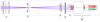 |
Fig. 2 MISTRAL optical scheme: (1) Focal reducer, (2) field lens −128 mm (with the slit a few mm before), (3) achromat collima-tor f = 200 mm, (4) filter wheel, (5) VPH 600 tr/mm with two prisms 19,8° (blue)/25,6º (red), and (6) 100 mm lens. |
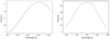 |
Fig. 3 Relative spectral response over the CCD 4000–10000 Å range. Left: blue dispersor and blue lens (from Feige 15 observations). Right: red dispersor and red lens (from BD+26, 2606 observations). |
2.3 Observing modes and available spectral dispersors
Several observing modes (Table 2) are possible with MISTRAL. They are accessible from a dedicated graphical user interface (GUI hereafter), which shows the position of the different ele ments in the optical path. These are the filters (with 12 positions), the spectral dispersors (blue and red volume phase holographic (VPH) gratings, to be used with the blue or red camera lens, respectively), and the slit (1.9 arcsec). These elements are sum marized in Table 1 and selected according to the different operating modes (imaging, spectroscopy, or setup).
The dispersor (blue or red) has to be chosen before the begin ning of the run so that the correct camera lens is mounted during day time. This will change in the future when a custom-made unique lens with a wide spectral coverage will be available, thus avoiding any dismounting of the instrument. In order to measure the CCD spectral response, several standard spectrophotomet-ric stars were observed. Figure 3 shows the computed spectral response for the blue dispersor and blue lens from Feige 15 observations (Stone 1974), and for the red dispersor and red lens from BD+26, 2606 observations (Oke & Gunn 1983). The total efficiency of the system (telescope + instrument + detector) is ~22% at peak (6000 Å).
Main characteristics of the MISTRAL instrument.
Main MISTRAL modes.
2.4 Exposure-time calculators
Exposure-time calculators are available remotely. One for spec-troscopy, ETC18, and one for imaging, ETC29. The details of the parameters that need to be entered into the calculators are described in the Appendix A, and some results are displayed there as well. We briefly describe what can be achieved.
For spectroscopy, we summarize in Table 3 the V-band mag nitudes detected with a total exposure time of one hour with an S/N of 3 for point-like objects under a median seeing (for OHP) of 2.5 arcsec, and with Moon conditions of 135° from the Moon and an illumination of 25%.
For imaging, ETC2 gives the exposure time needed to detect objects at a given magnitude with the requested S/N. While the details of the procedure are fully described in the appendix, we summarize the important results in Table 4.
See also MISTRAL CookBook10 (page 23) for the minimum possible exposure times.
2.5 Data archive
In addition to their local storage in the MISTRAL computers at the telescope, raw MISTRAL data are automatically archived within a database11 hosted by the CeSAM12. Raw data are visi ble but not accessible during a proprietary period of 12 months to anyone other than the principal investigators. All calibration data are immediately public. A possibility is also offered to the observers to store or make available their final reduced data and added values through the GASPIC national service13.
2.6 Expected optical improvement
In order to increase the instrument efficiency and avoid change-overs of optics when changing from blue to red settings (or vice versa), we are preparing a single camera lens covering the full MISTRAL spectral range. This is expected to be installed on the instrument in 2024 or 2025.
The new custom-made camera design consists of five lenses with two aspheric surfaces and uses low-dispersion OHARA S-FPL53 glass for the strong positive lenses. It is optimized to operate in the full working spectral range with a dispersed beam, which implies a forward-shifted entrance pupil.
The expected performance of the lens in development is compared to the performance of the commercial lenses that are currently used in the instrument. In the actual blue-visible set ting, an FX AF-S NIKKOR 105 mm f/1.4 lens is used, and its module transfer function (MTF hereafter) is available from the manufacturer at two reference spatial frequencies. In order to make a correct comparison, the calculations in the visible were made for the F, d, and C wavelengths (4860–6560 Å), and the field edge corresponds to 11° in each case. As the throughput curve for this Nikon lens is not available, it was estimated from the known number of surfaces and groups in the design, presum ing that the anti-reflective (AR) coating has a residual reflectance of 1% (similar to that in the custom design; see also MIS TRAL CookBook14 (page 20)) and the glass type composition is close to that used in [U.S.Patent 5572277]. The commercial lens data are taken from photographylife15. The throughput increases from about 75% to about 95% at 5000, 6000, or 7000 Å and markedly from 19 to 77% at 4000 Å, while the MTF decreases only marginally.
In the same way, the comparison was made for the Schneider Emerald 2.9/100 F-LD lens, which is actually used in the red range. This time, both the MTF and throughput are known from the product datasheet16. The foreseen transmission is similar to the current transmission at 7000 Å (93%), and slightly lower at 8000 Å (90% instead of 95%), with a decrease of a few percent of the MTF at 40l/mm. However, it should also be noted that the aperture of the current Schneider lens is insufficient and results in significant vignetting toward the edges of the spectrum, with a maximum loss of 40% at 6000 Å and 10000 Å. Thus, this vignetting loss will disappear with the new camera lens.
The nominal f-number, design wavebands, and the pupil positions are different for all these lenses, so that the compar ison is not straightforward. However, it indicates that the custom design is notable for an increased throughput in the shortwave visible range, and the contrast at medium spatial frequencies remains high even for a faster beam.
Typical spectroscopic limiting magnitudes corresponding to a total exposure time of one hour with an S/N of 3 for point-like objects under a median seeing of 2.5 arcsec, and with Moon conditions of 135° from the Moon and an illumination of 25%.
90% completeness for point sources under average imaging observing conditions at the OHP.
3 On-sky validations
To provide an impression of what is possible with MISTRAL, we report below salient (so far unpublished) examples of science made with MISTRAL observations during its first two years of exploitation. Following the main science goals of the instrument as described in the introduction, various types of objects were observed during several test periods, starting in April 2021 and lasting until around end of 2022, with progressively more science taking over the tests themselves. We describe some of the results obtained so far below.
We list in Table 5 the observing conditions of the spectra shown in Figs. 4–6, and 10.
3.1 Emission line stars: NovaCas 2021
V1405 Cas was discovered on 18 March 2021 and could be observed during the first commissioning nights of the instrument in April and July 2021. For instance, the spectra obtained on 5 July 2021 (i.e., about 100 days after maximum), still showed PCygni profiles in the H and He Balmer lines, which is a sign of the expanding envelope, but also some NII and FeII lines, indicating that the object was transiting from the He/N phase to the FeII phase. In Fig. 4 we show two spectra of this slow nova, which was later observed with both the blue and red MISTRAL grisms on 30 June and 28 June 2022, respectively, that is, about 415 days after maximum. The PCygni profiles no longer appear in these spectra, and the line profiles do not yet show a rectangu lar shape either. This confirms the FeII type. The line widths of the strong lines are measured at 1800 km/s FWHM. In addition to the H and He lines, the strong lines of [FeVII] are most con spicuous, in particular, those at 6086 and 5721 Å. On the other hand, the absence of the usually strong OI lines 8446 Å (and the weaker 7773 Å) is surprising: we have to wait for the nova to reach the full nebular phase for a proper abundance analysis.
3.2 General stellar classification: Bow shock stars
Bow shocks are arc-shaped structures located ahead of a star and are generally observed at mid- to far-IR wavelengths. They are expected to result from the interaction of the stellar wind with the ambient interstellar medium (ISM) when the star has a relative supersonic motion with respect to the ambient medium. Because the bow-shock driving star is expected to be an O- or B-type star, we led a spectroscopic follow-up of a sample of 47 bow-shock star candidates selected from the Jayasinghe et al. (2019) catalog that were selected to be observable with the MISTRAL instrument. Figure 5 shows a typical spectrum for a V = 9.7 star.
The spectral classification of stars is commonly made based on lines in the 4000–5000 Å domain, but due to the lower sensi tivity of the instrument in this spectral range, we performed the spectral classification from lines in the red part (4500–7000 Å) of the spectrum (Mk standards in the red were provided by, e.g., Danks & Dennefeld 1994). Of the 47 candidates, 2 are unclassi-fiable stars, 3 are cool stars, one is an A-type star, 10 are O stars, and 31 are В (mainly giants and supergiants) stars. This allows us to confirm that bow shocks are mainly driven by hot stars. The details of these results, complemented with a transverse velocity study (based on Gaia-DR3 astrometric data) of the stars, can be found in Russeil et al. (in prep.).
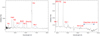 |
Fig. 4 Spectra of V1405Cas = NovaCas202l obtained in June 2022 with the blue (left) and red setting (right, enhanced y-scale). |
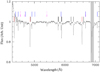 |
Fig. 5 Continuum-normalized spectrum of the candidate BS star 2G1045666+0128085 observed with MISTRAL. The position of the main lines used for the classification (the dashed magenta, blue, and red correspond to the HeII, HeI, and Balmer lines, respectively) and the diffuse interstellar bands (black dashes) is indicated. The vertical gray band underlines the night-sky feature. |
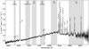 |
Fig. 6 MISTRAL spectrum of LkHα 324SE with telluric corrections, obtained with the red configuration and a single exposure of 900 s (of the two that were observed) on the night of 8 December 2021. The flux error bars are plotted in gray. The vertical light gray stripes indicate the atmospheric absorption bands of water and molecular oxygen. |
3.3 Red domain towards 1µ: The variable pre-main-sequence star LkHα 324SE in Lynds 988
Gaia2lfji17 (also known as AT2021aftk18 in the interna tional astronomical union: IAU designation) was reported on 6 November 2021 as the “brightening of a variable red Gaia source, candidate YSO (young stellar object)” (Hodgkin et al. 2021). We obtained a classification spectrum on 8 Decem ber 2021 with MISTRAL in the red configuration (Adami et al. 2021). Gaia2lfji corresponds to the emission-line star LkHα 324SE (Herbig & Rao 1972; Chavarria et al. 1983; also known as HB С 727 in Herbig & Bell 1988), which is a member of the pre-main-sequence population of the dark cloud Lynds 988, located at ~600 pc (Herbig & Dahm 2006). It is therefore not a new candidate YSO identified by Gaia. The spectrophotometric standard Feige 15 was observed after LkHα 324SE (Appendix D).
The spectrum displays many strong emission lines above a red continuum (Fig. 6): Hα, Paschen (Pa) lines, the Ca II infrared triplet (IRT), and the O I λ8446. Fainter emission lines of Mg I, Fe I, and Fe и are also detected, in addition to the for bidden O I lines. The O I λ7772 absorption triplet is detected. The Ca II IRT in emission is an indicator of chromospheric activ ity and potentially of accretion (Mohanty et al. 2005; Yamashita et al. 2020).
The emission lines Pa 8–12, 14, and 17 are detected. The Pa 8–10 lines are located in the MISTRAL spectrum region that is strongly affected by fringing (see also MISTRAL CookBook19 page 16 and test report20 page 15) and the water absorption band. The measured equivalent widths (EW hereafter) might therefore be sensitive to the determination of the pseudo-continuum and the correction of the telluric absorption. Pa 16 λ8502.27, Pa 15 λ8545.17, and Pa 13 λ8664.80 cannot be resolved with MIS TRAL from the emission lines λλ8498.02,8542.09, and 8662.14, respectively, of the Ca II IRT (see bottom panel of Fig. C.1). However, Pa 18 λ8437.75 and O I λ8446.76 are 9.01 Å apart, which is just large enough for them to be barely resolved as the MISTRAL FWHM is 8.5 Å at this wavelength (see the bot tom panel of Fig. C.1). Figure 7 shows the MISTRAL spectrum centered on the O I λ8446.76 with a hint of Pa 18 on its red wing.
Herbig & Dahm (2006) also identified the [S II], [O I], and [N II] lines from LkHα 324SE; the [O I] λλ63OO, 6363 lines have the same shape as the [S II] λλ6717, 6730 lines, which display a narrow component at −18 km s−1 superposed on a very broad asymmetric line that peaks near −200 km s−1 (their Fig. 12, bottom panel). The [O I] high- and low-velocity components of Τ Tauri stars are associated with microjets and disk winds, respectively (Hartigan et al. 1995). The [N II] λλ6548, 6583 lines cannot be resolved with MISTRAL from the broad wings of the Hα line. The [S II] λλ6717, 6730 lines are not detected with MISTRAL, but our 1.9″-slit was oriented NS, not at a position angle of 309° along the NW flow, as in Herbig & Dahm (2006), which may dilute the observed flux from the base of the NW flow. Figure 8 shows the regions of the [O I] λλ6300.23, 6363.88 lines with two faint emission lines with an equivalent width (EW) of −1.6 and −0.3 Å, respectively. These faint lines are blueshifted, with velocity shifts that are consistent with the high-velocity broader component of these lines. Therefore, MISTRAL can also detect faint forbidden [O I] lines from this pre-main-sequence star.
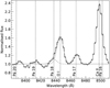 |
Fig. 7 Pa 18 λ8437.75 and ΟI λ8446.76 from LkHα 324SE. The solid gray line is the combined Gaussian best fit of these two lines. The dashed gray lines are the individual Gaussian best fits of these two lines. They confirm the detection of the Pa 18 line (see text for details). |
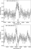 |
Fig. 8 Faint blueshiſted [O I] emission lines from LkHα 324SE. The dotted step line in the top panel shows the normalized spectrum without correction of the atmospheric O2 γ band. The gray line is the Gaussian fit. The quoted error of the velocity shift includes the wavelength cali bration error in quadrature. |
3.4 Test of the spectral resolution of MISTRAL around the Нα line in LkHα 324SE
In MISTRAL observations of LkHα 324SE, the Hα line is strong, with an EW of −107 Å, which is well above the maximum Нα EW of −20 Å that can be produced by an active stellar chromosphere in later-M spectral-type stars. The origin of this emission therefore is an accretion shock at the stellar surface (Muzerolle et al. 2001). Moreover, the Нα line is broad with an FWHM(Hα) = 13.98 + 0.05 Å (Fig. 9), which is far larger than the MISTRAL spectral resolution of 7.9 Å for the red con figuration (Eq. (C.2)). The (deconvolved) full width at 10% of the Нα peak is 961 + 5 km s−1 (Eq. (C.3)), which is larger than the minimum value of 270 km s−1 that is used as accre tion criterion in low-mass stars (White & Basri 2003). We note small residuals between the MISTRAL Нα line and the Gaussian fit that suggest an asymmetric profile for this line. The high-resolution (R ~ 45 000) spectra of LkHα 324SE, obtained on 6 July 2003 and 13 December with the HIgh-REsolution Spec trograph (HIRES) at the Keck I telescope on Mauna Kea, shows the Hα line (Fig. 10, top panel of Herbig & Dahm 2006) with an EW of −170 Å, wings extending to +550 km s−1 at least, and an absorption component at −114 km s−1, which is usually associated with a stellar wind, between the secondary and main line peaks at −200 and 2 km s−1, respectively. We note that the secondary peak is less than half the strength of the primary peak. This classies this Hα line as a type IIIB profile, which is the most common profile (33%) in Τ Tauri stars, whereas it is three times less common (11%) in Herbig Ae/Be stars (Reipurth et al. 1996).
A medium-resolution (R = 5000) spectrum in the blue of LkHα 324SE was obtained by C.A. 12 days after the MIS TRAL observation on the night of 20 December 2021 with the AURELIE spectrograph at the OHP 1.52 m telescope (Gillet et al. 1994). This AURELIE spectrum will be reported else where. Here, we focus on the Hα line observed with AURELIE (Fig. 9). This type IIIB profile line displays an EW of −119 Å, that is, 43% fainter and 10% stronger than during the HIRES and MISTRAL observations, respectively; and an absorption component at −52 km s−1, that is, twice less blueshifted than observed 18 yr before; secondary and main-line peaks at −174 and 112 km s−1, respectively, that is, less blueshifted and much more redshifted than observed 18 yr before. The Imax/40 veloc ities (Reipurth et al. 1996) for the blue and red wings are −507 and 601 km s−1, respectively. We used the shape of the AURE LIE Hα line as template for a comparison with the MISTRAL Hα line. After convoluting (Gaussian with σ = 3.3 Å from the quadratic combination of the resolution) and resampling (2 Å spectral bins) this template, the best-fit match with the MISTRAL Hα line was obtained for a velocity shift of about −227 km s−1. However, this high value of the required velocity shift suggests a strong variation in the shape of the Hα line on a timescale of 12 days, including, for instance, a more blueshifted absorption component during the MISTRAL observation.
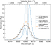 |
Fig. 9 Broad and variable Нα emission line from LkHα 324SE. The black data with error bars are the normalized MISTRAL spectrum. The gray line is the Gaussian fit of the emission line. The solid blue line is the medium-resolution (R ~ 5000) spectrum obtained 12 days after the MISTRAL observations, with the OHP 1.52 m telescope with the AURELIE spectrograph. The dotted blue line shows the same spec trum shifted by −227 km s−1 to match the position of the emission line observed with MISTRAL. The orange line is the convolved (Gaussian with σ = 3.3 Å) and resampled (2 Å spectral bins) AURELIE spectrum to match the spectral resolution and sampling of MISTRAL. |
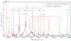 |
Fig. 10 Observations of comet C/2022 E3 (ZTF). Black line: optical spectrum observed with MISTRAL spectrograph camera on the OHP telescope. The spectra, obtained from the 240s frame, were extracted using a 29.2arcsec × 1.93 arcsec aperture with the comet at the center. The dashed red line shows the spectrum obtained from the HCT tele scope (priv. comm.). The typical bright cometary bands such as C2 and NH2 are well visible in the spectrum after proper subtraction of the solar continuum and sky lines. |
3.5 Solar System objects: Comet C/2022 E3 (ZTF)
The bright comet C/2022 E3 (Zwicky Transient Facility: ZTF) was observed in manual tracking mode for two exposure times, 120 and 240 s, using the MISTRAL spectrograph camera on the 1.93 m OHP telescope on 10 February 2023, when the comet was at a distance of 1.20 AU from the Sun and 0.39 AU from the Earth. We used the blue mode, covering the ~4200–8000 Å range at a resolution of ~750 with a slit of l.9arcsec. All the acquired frames for different exposures were bias subtracted and then flat fielded using the spectral flat lamp present in the instrument (Tungsten). The cosmic rays were removed using the LACOSMIC package (van Dokkum 2001). The reduced and extracted ID spectrum is shown in Fig. 10.
The 120 and 240 s spectra, even if slightly trailed, were both used to compute the production rates of the C2 (Δν = 0) emis sion band using a single aperture (200 pixel aperture) with the comet at the center, as mentioned in Aravind et al. (2021). The 120s spectra were better guided with a narrower dust continuum. They were used to extract spectra with apertures of equal widths moving away from the photocenter to compute the spatial profile of the column density and hence the production rates with the help of Haser (1957) modeling. The spectrophotometric stan dard, Hiltner6OO, observed on the same night using the same configuration, was used to produce the sensitivity curve of the instrument and to then flux calibrate the comet spectra. The solar analog standard star HD 19445 was observed on the same night to remove the dust-reflected solar continuum present in the opti cal spectra. Even though a separate sky frame of similar exposure is ideally required to remove the sky background from the comet frames, we used the sky from a point source observed with a similar exposure time on the same night to remove the sky lines.
Several typical cometary emission bands were detected from C2, NH2, and CN radicals. The production rates of (2.61+/−0.04)E26 and (2.51+/−0.07)E26 for C2 (Δν = 0) were computed for the 240s frame and 120s, respectively, and agree well with the values reported for the same comet from the TRAP PIST telescopes (Jehin et al. 2022, 2011). The Afρ, a proxy of the dust production (A’Hearn et al. 1984) computed for the green continuum narrow band filter (Farnham et al. 2000), from spectroscopic data using techniques as described in Aravind et al. (2022), was found to be around 5100±80 cm, which again agrees with the values reported from TRAPPIST for the comet at similar observational epochs.
As a comparison, we also show in Fig. 10 the spectrum obtained for comet C/2022 E3 from the 2-meter class Himalayan Chandra telescope (HCT, priv. comm.). This telescope uses the Hanle Faint Object Spectrograph and Camera (HFOSC) and cov ers a wavelength range of 3750–6850 Å. The comparison shows the good resolution of MISTRAL, which shows the emission lines in a sharper way. MISTRAL also reaches deeper in the red, but misses the blue part of the spectrum with the bright CN line, which is well visible in the HCT spectrum. Among other items, this justifies the new lens we are developing, which will be more efficient toward the blue.
With the help of these OHP observations, the MISTRAL spectrograph camera on the OHP telescope proves to be reliable for cometary observations for a wavelength range of 4200 8000 Å. With proper differential tracking and when the required frames are acquired in an orderly manner, longer-exposure obser vations of fainter and more distant comets could be used to effectively analyze the column density profiles of the various emission bands marked in the figure, which can further be used to compute their production rates.
4 Main targets of MISTRAL: GRB follow-up program
The MISTRAL instrument is well-suited for studying the GRB physics (see, e.g., Schneider et al. 2023b) as it combines a low-resolution spectroscopic mode (with a blue and red range) that is sufficient to infer their redshift using absorption lines in the afterglow emission and an imaging mode that allows character izing their optical and near-IR temporal evolution. The French GRB community has proposed a dedicated MISTRAL ToO pro gram in order to characterize the afterglow emission of the well-localized bursts detected by the BAT and XRT high-energy instruments on board the Neil Gehrels Swift space observatory (Gehrels et al. 2004). This program is a preparation for the future exploitation of the Sino-French SVOM mission, which is expected to be launched in June 2024 (Wei et al. 2016), and has been conducted since March 2022.
We currently have strict trigger criteria to avoid disturbing the other observing programs too much, but in practice, they can be relaxed for important events (e.g., following information reported by other teams via Gamma-ray Coordination Network (GCN) circulars21), and they will need to be revised when SVOM is operational. We have observed 21 GRBs so far, as shown in Table 6.
Most of the observed GRBs in Table 6 were day-time trig gers, which explains the relatively long delay between trigger and MISTRAL observations. This is due to the pointing strat egy of the Swift spacecraft, which can detect bursts near the Sun. In contrast, SVOM has an optimized anti-solar pointing strat egy, which will result in detections of GRBs only during the night on Earth and will thus enhance the rates of fast follow-up at the OHP site. Few GRBs were observed with very long latency (GRB 221009A and AT2023lcr) because newly received information (updated position and flux measurements) allowed us to identify these events as interesting targets. The only (Swift) night-time trigger so far was GRB 240218A, which we were able to observe 30 min after the alert. We could be faster in principle, but the telescope rules impose that the exposure of the ongo ing regular observing program is completed if fewer than 30 min remain. This therefore mechanically limits the reaction time to ~30 min.
4.1 Data analysis
For each GRB MISTRAL ToO, we start with a typical sequence of r-band images in order to detect the source and then to accurately place the slit at the correct GRB location. If the GRB remains too faint or undetected after these first images we continue to observe in imaging mode to reach a higher sensi tivity. If the GRB is detected and bright enough compared to the MISTRAL spectroscopic limiting magnitude (r < 19–20), we perform spectroscopic observation for about one hour to obtain a good S/N spectrum of the source. Both the photomet ric and spectroscopic data are reduced immediately in order to communicate our results in real time to the scientific community.
4.2 Data reduction
We first preprocess the MISTRAL raw images with the appro priate bias and flat-field calibration images. The single-exposure images are then astrometrically solved and coadded to be ana lyzed. The GRB positions were known at an arcsecond accuracy level, which allows us to directly perform forced photometry. To do this, we use the simple transient detection pipeline, STD-PIPE, (Karpov 2021). Our photometric analysis follows the steps described below (and in the git documentation22 of the STDPIPE project).
- 1.
We mask the saturated stars, the cosmic-ray artifacts, and the bad columns of pixels.
- 2.
We extract the point-like sources (S/N > 3) using SEX-TRACTOR (Bertin & Arnouts 1996).
- 3.
We calibrate the photometry of the sources using the PHO-TUTILS23 Astropy package (Bradley et al. 2021). We use the Panoramic Survey Telescope and Rapid Response System (PanSTARRS) DR1 catalog (Chambers et al. 2016) as a ref erence, a cross-match radius of 2 arcseconds to associate the cataloged sources with our SEXTRACTOR ones, and a flux aperture radius ~ 1.5 × FWHM (the mean of the full width at half maximum of the image sources). The local background was measured in an annulus of [3–5] × FWHM.
- 4.
To reduce the flux contamination from nearby sources or the GRB host galaxy (if visible in the images), we may perform a difference-image analysis using the code HOTPANTS (Becker 2015) and the CDS HIPS2FITS service (Boch et al. 2020).
- 5.
If the source is detected in the coadded image, we perform forced-aperture photometry at the GRB location using the same aperture configuration as during the calibration steps.
- 6.
If the source is not detected, we estimate the upper limit from the local background for a source that would have given a positive detection at a given S/N.
For spectroscopy, we use the night-time dedicated MIS TRAL spectroscopic pipeline24, which is based on the software ASPIRED (Lam et al. 2023).
GRBs followed-up at OHP using the MISTRAL instrument mounted on the 193 cm telescope during semesters 2022A, 2022B, 2023A, and 2023B.
4.3 Results
For 9 out of 21 (~45%) of our follow-up campaigns, we were able to clearly identify and measure the brightness of the GRB after glow. These 9 include AT2023sva (Parra-Ramos et al. 2023), a GRB afterglow without any high-energy trigger that was initially discovered in ZTF survey data from blind searches for fast opti cal transients (Vail et al. 2023). We also covered several obser vational epochs for the brightest GRB of all time (the BOAT), GRB 221009A, and for the third-brightest Fermi-GBM burst, GRB 230812B (OHP data reported in Hussenot-Desenonges et al. 2024). Section 4.4 describes our photometric results for GRB 221009A in more detail.
In addition, we were able to trigger four times the spectro-scopic mode of MISTRAL to characterize the transient or to infer the redshift of the potential host galaxy for GRB 230427A (Adami et al. 2023e), for GRB 230506C (Adami et al. 2023c), and for the orphan afterglow AT2023sva (Parra-Ramos et al. 2023). For the GRB 230506C, we suggest a redshift of 3.7 ≤ z ≤ 4. This is the only redshift measurement reported for this burst, and it also represents the most distant redshift measured at OHP so far. The spectrum of GRB 230506C shows the capabili ties of MISTRAL at its limits, securing a tentative spectroscopic redshift measurement for a source at magnitude r ~ 20.9 with a total exposure time of 30min (blue dispersor). The redshift was determined taking advantage of a break at around 6000 Å, which was interpreted as the Lyman-α break (see Fig. 11). For the 12 undetected of the 21 GRBs, we were able to place interesting constraints on their optical flux evolution, as shown in Fig. 12 in the r band.
4.4 GRB 221009A: The BOAT
GRB 221009A was triggered by the Gamma-ray Burst Monitor (GBM) instrument on board Fermi (Veres et al. 2022; Lesage et al. 2023). It was detected since then during days to weeks at all wavelengths, including at TeV energies (Fulton et al. 2023; Laskar et al. 2023; Williams et al. 2023; Aharonian et al. 2023; Levan et al. 2023; An et al. 2023; Kann et al. 2023; Cao et al. 2023). It was rapidly established that the properties of this burst were extraordinary given its intense luminosity and close distance (i.e. z = 0.151, Malesani et al. 2023). Many aspects of the physics of GRB 221009A, regarding the nature of the GRB relativistic jet and its angular structure, the efficiency of the kinetic to radiation conversion mechanisms of the jet and the afterglow radiation model (Gill & Granot 2023; Zheng et al. 2024; O’Connor et al. 2023; Ren et al. 2024; Zhang et al. 2024; Dai et al. 2023), or the Lorentz invariance principle (Vardanyan et al. 2023; Finke & Razzaque 2023; Piran & Ofengeim 2024; Yang et al. 2024), have been highly debated in the scientific community. These discussions will continue in the upcoming months and years because an event like this is thought to occur only once every 10 000 yr (Burns et al. 2023) and is therefore a rare opportunity for studying GRB physics in great detail. In this very active context, we have performed two epochs of photometric observations at about 6 and 10 days after the Fermi-GBM trigger time, complemented with three epochs with the 120cm telescope at the OHP (Schneider et al. 2022a). In Table 7, we summarize our photometric results, and we show them in the context of the worldwide follow-up campaigns in Fig. 13.
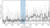 |
Fig. 11 Spectrum of GRB230506C taken by MISTRAL (30 min exposure). The thin black curve represents the full spectrum, and the thick black curve represents the spectrum rebinned by 20 pixels. The gray shaded area represents the error spectrum. The center of the expected Ly α positions for z = 3.7 and z = 4 is shown as the vertical blue line. The blue shaded area represents the possible values of the Ly α centroid, assuming that the drop at 6100 A is due to the Lyman break. |
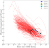 |
Fig. 12 Comparison of the MISTRAL GRB afterglow detections (colored circles) and upper limits (black triangles) with respect to the known population of GRB afterglows (1997–2023: not a complete sample). |
Optical and near-IR observation of ORB 221009A with the T193/MISTRAL and T120 telescopes located at the OHP.
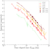 |
Fig. 13 Optical and near-IR afterglow light curve of GRB 221009A. The OHP observations (T193/MISTRAL and T120) are shown as colored pentagons. The literature data are collected from Fulton et al. (2023); Laskar et al. (2023). |
5 Conclusions
The spectro-imager MISTRAL has been installed at the folded Cassegrain focus of the 1.93 m telescope at the Haute-Provence Observatory in 2021 and is running smoothly. It covers the spectral range from 4000 to 10 000 Å in two settings, blue or red, at an average spectral resolution of 700. At the moment, two grisms and five broadband filters (g′, r′, i′, z′, Y) are available, plus some narrowband filters around the main emission lines. Room is available for more grisms and filters to be installed in the future. The total throughput has been measured around 22% at the peak efficiency of 6000 Å, with the current deep-depletion CCD of 2048 pixels of 13.5 microns each. The efficiency rapidly drops below 4000 Å due to the poor transmission of the actual blue camera objective, but this will be replaced by a custom-made new objective that will cover the full spectral range, avoiding time-consuming changeovers. A limiting magnitude of r ~ 19 can be obtained in one hour of spectroscopy, while limiting magnitudes in the range of 20–21 are achieved in imaging mode in 10–20 mn exposures, depending on the exact filter and local seeing conditions. A specific interface is available, showing the nature and position of all optical elements, making the instrument very user-friendly. It can be put into operations in less than 15min (change-over from the other, permanently mounted instrument, Sophie), as required by the scientific program. On-sky tests with various types of objects have shown the operability and versatility of MISTRAL: we presented a few examples of emission line stars, novae, young stellar objects, or galaxies, with particular emphasis on the follow-up of GRBs, which are likely to become a major source of targets with the launch of the SVOM satellite in 2024.
Acknowledgements
Authors acknowledge the efficient support of the OHP night operators, in particular J. Balcaen, Y. Degot-Longhi, S. Favard, and J.P. Troncin. Based on observations made at Observatoire de Haute Provence (CNRS), France, with MISTRAL on the T193 telescope, with AURELIE on the T152 telescope and with the CCD camera of the T120 telescope. We warmly thank Marco Lam for his contribution to the MISTRAL spectroscopic reduction software. We also acknowledge very useful discussions, during the conception phase, with the SPRAT team, in particular Iain Steele and Andrzej Piascik. This research has made use of the MISTRAL database, operated at CeSAM (LAM), Marseille, France. Authors thank the CPER OHP2020 Région Sud and the Conseil départemental des Alpes de Haute Provence for their contribution. This work received support from the French government under the France2030 investment plan, as part of the initiative d’Excellence d’Aix-Marseille Université – A*MIDEX (AMX-19-IET-008). We were also supported by the IPhU Graduate School program at Aix-Marseille University. EJ is a FNRS Senior Research Associate. TRAPPIST is a project funded by the Belgian Fonds (National) de la Recherche Scientifique (F.R.S.-FNRS) under grant T.0120.21. We also acknowledge the support by Master Erasmus Mundus Europhotonics (599098-EPP-1-2018-1-FR-EPPKA1-JMD-MOB) financed by EACEA (European Education and Culture Executive Agency). Authors thank the CNES for financial support of the MISTRAL operations. Authors thank the former Pythéas institute director, N. Thouveny, for his great contribution to the MISTRAL instrument. Authors thank T. Adami and J. Hornstein for their contributions to the GRB alert system and the data reduction tools. Authors thank A. DelSanti for useful discussions for the C/2022 E3 (ZTF) comet observations.
Appendix A Exposure time calculators
We describe below the various parameters needed for the exposure time calculators to operate, and how we obtained the results we presented. ETC1 is for spectroscopy, and ETC 2 is for imaging. We note that the ETCs will be updated when the single lens described in Section 2.6 is installed on the instrument.
Appendix A.1 Spectroscopy
ETC1 requires several parameters: the choice of grating (blue/red), the expected seeing, the target V-band magnitude, the required S/N for the expected most intense spectral line, the nature of this line (absorption or emission), and the physical shape of the target (point source or extended source, modeled by a Gaussian). ETC1 basically uses an N-parameter space of these parameters and fits a model at the place of the target in the considered space in order to give an exposure time.
ETC1 also requires (1) the Moon conditions in terms of Moon illumination (choice between 0.25 , 0.5 , 0.75, and 1) and the angular distance of the object to the Moon (choice between 45°, 90°, 135°, and 180°), (2) the extended (or not) nature of the object, and (3) if needed, the intrinsic FWHM of the object if modeled by a Gaussian. This is the angular size of the object before seeing convolution. At this step, ETC1 computes the percentage of the flux that arrives on the CCD after convolution of the object signal by the seeing and the slit (1.9arcsec wide at the moment). This percentage is applied to the given target magnitude. (4) The air mass (using the OHP extinction curve). Additional extinction in magnitude can also be added to take potential cloud-induced extinction into account.
ETC1 is now able to fit a model to real observations within the adapted space in order to give an estimated exposure time. 3D views similar to those in Fig.A.1 are also provided to allow the observer to manually adjust their exposure-time estimate as a function of the location of the target in the 3D sheet (see Fig. A.1).
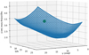 |
Fig. A.1 Example of ETC 3D sheet within the (magnitude, S/N, exposure time) space for the blue setting. |
Appendix A.2 Imaging
Another exposure time calculator (ETC2) is available to give to the observer a typical exposure time for their targets in imaging mode. ETC2 gives the exposure time needed to detect objects at a given magnitude with the requested S/N.
These estimates are based on observations of several fields (XCLASS3091 cluster of galaxies, Koulouridis et al. (2021), Abell400 cluster of galaxies, and at2021ft transient field) observed in g′,r′, i′, z′, and Y bands under different seeings and airmasses. They were observed with different exposure times of between 1 min and 60 minutes. They were all at relatively low galactic latitudes, providing catalogs of several hundred stars. These stars were separated from galaxies using the SDSS images available for these fields. We used simulations to degrade the shape of these stars before we redetected them (to take the seeing and object extension into account). ETC2 then uses an N-parameter space of these characteristics and fits a (second-order) polynomial function for the place of the target in order to give an exposure time.
Similarly to ETC1, the technique used to generate an exposure time typically consists of the following steps: (1) select the filter to be used in imaging. (2) give the expected seeing, (3) give the extended (or not) nature of the object (4) if needed, give the intrinsic FWHM of the object if modeled by a Gaussian; this is the angular size of the object before seeing convolution, (5) give an additional extinction in magnitudes to take a potential cloud-induced extinction into account, (6) give the air mass to compute the magnitude loss due to the atmosphere (using the OHP extinction curve), (7) give the target magnitude, and (8) give the required S/N.
ETC2 is now able to fit a polynomial model on real observations within the chosen space in order to give an estimated exposure time. 3D views similar to those in Fig.A.1 are also provided to allow the observer to manually adjust the exposure-time estimate as a function of the location of the target in the explored space. ETC2 will give the exposure time needed to detect objects at the required magnitude for an S/N higher than required.
Appendix B Filter responses
The filter responses25 are summarized in Table B.1 and shown in Fig.B.1.
The MISTRAL filter transmission was measured with the Laboratoire d’Astrophysique de Marseille Perkin-Elmer spectrograph between 4000 and 10000 Å using the PMT and InGaAs sources and low (4 Å) and high (2 Å) resolution. The wide-range filters (g’, r’, i’, z’, Y, passe-haut 4000-10000 Å, passe-haut 6000-10000 Å) were measured with a resolution of 4 Å (one measured point every 2 Å with a measured width of 4 Å). The narrowband filters (Hß, OIII, Hα, SII) were measured with same setup between 4000 and 10000 Å and with a better resolution of 2 Å (one measured point every Å with a measured width of 2 Å) around their useful domain.
MISTRAL filter response functions.
The accuracy of the measurements was evaluated by comparing the results between two consecutive measures (without filter repositioning between two measures) and was estimated with the SII filter measured at high resolution. The difference between two consecutive measures is well below the 1% level, and the shift in wavelength is lower than 0.1 Å.
Appendix C MISTRAL spectral resolving-power estimates
The spectral resolving power, R = λ/FWHM with FWHM the full width at half maximum of the sharp line (Robertson 2013), was computed for the blue and red configurations of MISTRAL (Table C.1). The linear fitting of these data (Fig. C.1) provides the following formulae of R versus the wavelength for the blue and red configurations, normalized at the wavelength of the Hα line:
 (C.1)
(C.1)
 (C.2)
(C.2)
Therefore, the spectral resolving power at the Hα line is ~7% better in the red configuration.
From high-resolution (R ~ 33,000) optical spectra of T Tauri stars and brown dwarfs, it was demonstrated empirically that the full width at 10% of the Hα emission profile peak (hereafter, FW10%Hα) can be used as an indicator of accretion when it is larger than 270 km s–1 (White & Basri 2003). To use this criterion with a MISTRAL spectrum, the observed Hα FWHM must first be corrected for the MISTRAL (Gaussian) line-spread function to estimate the intrinsic FWHM of Hα:  . Then, using FW10%Hα =
  , we derive the velocity width corresponding to FW10%Hα versus the observed Hα FWHM:
 (C.3)
(C.3)
with c the speed of light.
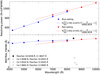 |
Fig. C.1 Theoretical spectral resolving power of MISTRAL. The data for the blue and red configurations are from Table C.1. Top panel: Resolving power vs. wavelength. The straight lines are the linear fitting of these data. Bottom panel: FWHM vs. wavelength. The curves are computed from the linear fits. For comparison, the wavelength separation of several close stellar emission lines is marked with a diamond (resolved with MISTRAL) and crosses (unresolved with MISTRAL). |
MISTRAL theoretical spectral resolving power.
Appendix D Spectrograph sensitivity and telluric corrections using Feige 15 in the red configuration of MISTRAL
The spectrophotometric standard Feige 15 is a faint, blue star of the galactic halo (Feige 1958). The determination of its spectral type has evolved from A1 V (Sargent & Searle 1968) to sdA0IV:He1 (Drilling et al. 2013). Its spectral energy distribution (SED) is only reported from 3200 to 8370 Å (Stone 1977), using bandwidths of 49 Å and 98 Å in the wavelength ranges 3200–5263 and 5263–8370 Å, respectively (Stone 1974). Therefore, Feige 15 is routinely used for the spectral calibration of MISTRAL in the blue configuration, but its SED must be extended above 8370 Å to be used in the red configuration.
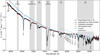 |
Fig. D.1 Red configuration spectrum of the spectrophotometry standard Feige 15 with MISTRAL, obtained with an exposure of 600 s on the night of 8 December 2021 (no telluric correction). The flux error bars are plotted in gray. The vertical light-gray stripes indicate the atmospheric absorption bands of water and molecular oxygen (Lu et al. 2021). The reference flux and bandwidth wavelengths are marked in red (Stone 1977, shortward of 8370 Å). The solid and dotted blue lines are the α Lyrae (Vega) CALSPEC spectrum and continuum (Bohlin et al. 2014), respectively, normalized at the wavelength and flux marked by the green plus. |
We adapted the get_sensitivity function of ASPIRED26 (Lam et al. 2023) to use the bandwidths of the reference fluxes when we determined the spectrograph sensitivity from the standard spectrum. We wrote a custom Python script to use the CALSPEC27 spectrum of α Lyrae (Vega), normalized on the bandwidth centered at 8370 Å, to extend the SED longward. We computed the fluxes of this A0 template within bandwidths of 25, 100, and 100 Å centered at 8807 (mean of the Pa 11 and Pa 12 wavelengths), 9740, and 9850 Å, respectively, outside the atmospheric absorption band of water (Lu et al. 2021), which leads to 10.679, 10.780, and 10.800 ABmag, respectively.
Fig. D.1 shows the reduced spectrum of Feige 15 as observed at an airmass 1.16, where the standard fluxes match the literature fluxes (Stone 1977) plus these three new references of flux. The observed depths of the Paschen lines outside the atmospheric absorption band of water match the A0 template very well, which can hence also be used for telluric correction in this atmospheric absorption band.
We estimated the standard continuum shortward of 8370 Å after excluding the atmospheric absorption bands. The ratio inside the atmospheric absorption bands of the standard continuum (shortward of 8370 Å) or the A0 template (longward of 8370 Å) and the observed flux were used for the telluric correction of the spectrum of LkHα 324SE (Fig. 6).
Appendix E CCD reading modes
Several CCD reading modes are available (nominal temperature of the CCD: ~-90C, saturation level: ~60 000). Two modes have been extensively tested, and they alone are offered: fast mode (3 MHz), and slow mode (50 kHz). They are briefly described in Table E.1. The fast mode is adapted for technical operations such as telescope focus or pointing, thanks to the very short reading time that allows real-time object focusing, for example. For science operations, a slow mode is offered with a read-out noise that is almost three times lower.
Characteristics of the different reading modes.
Appendix F Instrument stability
One of the science goals of MISTRAL is the long-time follow-up of variable objects. It therefore is important to evaluate its stability over time.
We therefore investigated the CCD mean electronic noise level with the 760 measured bias frames over an operating period of about 3 years. Fig. F.1 shows the variation in the mean ADU level and of the 1er mean level uncertainty of the biases over a period of 1050 days. Both are compatible with no variation over time, with a bias level of 302±6 ADUs.
We then investigated the response of the CCD when it was illuminated by an artificial source (to avoid sky variability and coating variations in the telescope primary mirror). We used the 917 available arc calibration frames for this and only selected the 30sec exposures made with the blue dispersor. Fig. F.2 shows the variation in the mean flux level of these exposures (upper panel). After an initial decrease of 15% in the flux during the first year, which is probably due to the aging of the wavelength calibration lamp, the mean flux has remained constant for almost 2 years.
We finally estimated the variation in the percentage of low-response CCD pixels. For each arc frame, we computed the number of pixels with an ADU level below 320. This corresponds to the mean bias level plus 3e . Every pixel below this level may be a low-response pixel because it is still compatible with a bias level despite the 30sec exposure with the calibration lamps “on”. Fig. F.2 shows a very low and stable level of these pixels, around 0.2% of the total number of CCD pixels.
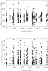 |
Fig. F.1 Variation over time (starting at the Julian Date of 2459310) of the mean ADU level (top panel) and of the 1er mean level of the uncertainty (bottom panel) of the MISTRAL biases. |
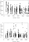 |
Fig. F.2 Variation over time (starting at the Julian Date of 2459310) of the mean ADU level (top panel) of the arc exposures of MISTRAL. The bottom panel shows the percentage of potential low-response pixels over time. |
References
- Adami, C., Grosso, N., Dennefeld, M., et al. 2021, ATel, 15131 [Google Scholar]
- Adami, C., Adami, T., Schneider, B., et al. 2023a, GRB Coordinates Network, 34418 [Google Scholar]
- Adami, C., Amram, P., Basa, S., et al. 2023b, GRB Coordinates Network, 34743 [Google Scholar]
- Adami, C., Basa, S., Le Floc’h, E., et al. 2023c, GRB Coordinates Network, 33741 [Google Scholar]
- Adami, C., Cuillandre, J. C., Ollivier, M., et al. 2023d, GRB Coordinates Network, 34247 [Google Scholar]
- Adami, C., Garnichey, M., Michel, F., et al. 2023e, GRB Coordinates Network, 33707 [Google Scholar]
- Adami, C., Le Floc’h, E., Götz, D., et al. 2023f, GRB Coordinates Network, 35286 [Google Scholar]
- Adami, C., Palmerio, J., Vergani, S. D., etal. 2023g, GRB Coordinates Network, 33749 [Google Scholar]
- Adami, C., Schneider, B., Basa, S., et al. 2023h, GRB Coordinates Network, 33607 [Google Scholar]
- Adami, C., Schneider, B., Birlan, M., et al. 2023i, GRB Coordinates Network, 33537 [Google Scholar]
- Adami, T., Adami, C., Turpin, D., et al. 2023j, GRB Coordinates Network, 34030 [Google Scholar]
- Adami, C., Le Floc'h, E., & Mistral Grb Collaboration 2024a, GRB Coordinates Network, 35744 [Google Scholar]
- Adami, C., Russeil, D., LeCoroller, H., et al. 2024b, GRB Coordinates Network, 35690 [Google Scholar]
- Aharonian, F., Ait Benkhali, F., Aschersleben, J., et al. 2023, ApJ, 946, L27 [NASA ADS] [CrossRef] [Google Scholar]
- A’Hearn, M. F., Schleicher, D. G., Millis, R. L., Feldman, P. D., & Thompson, D. T. 1984, AJ, 89, 579 [Google Scholar]
- Amram, P., Adami, C., Basa, S., et al. 2023, GRB Coordinates Network, 34762 [Google Scholar]
- An, Z.-H., Antier, S., Bi, X.-Z., et al. 2023, arXiv e-prints [arXiv:2303.01203] [Google Scholar]
- Andrillat, Y., Baranne, A., & Houziaux, L. 1975, A&A, 41, 99 [NASA ADS] [Google Scholar]
- Aravind, K., Ganesh, S., Venkataramani, K., et al. 2021, MNRAS, 502, 3491 [Google Scholar]
- Aravind, K., Halder, P., Ganesh, S., et al. 2022, Icarus, 383, 115042 [NASA ADS] [CrossRef] [Google Scholar]
- Basa, S., Adami, C., Degot-Longhi, Y., et al. 2023, GRB Coordinates Network, 35384 [Google Scholar]
- Becker, A. 2015, Astrophysics Source Code Library [record ascl:1504.004] [Google Scholar]
- Bertin, E., & Arnouts, S. 1996, A&AS, 117, 393 [NASA ADS] [CrossRef] [EDP Sciences] [Google Scholar]
- Boch, T., Fernique, P., Bonnarel, F., et al. 2020, ASP Conf. Ser., 527, 121 [NASA ADS] [Google Scholar]
- Bohlin, R. C., Gordon, K. D., & Tremblay, P. E. 2014, PASP, 126, 711 [NASA ADS] [Google Scholar]
- Bradley, L., Sipocz, B., Robitaille, T., et al. 2021, https://doi.org/18.5281/zenodo.4624996 [Google Scholar]
- Burns, E., Svinkin, D., Fenimore, E., et al. 2023, ApJ, 946, L31 [NASA ADS] [CrossRef] [Google Scholar]
- Cao, Z., Aharonian, F., An, Q., et al. 2023, Sci. Adv., 9, eadj2778 [CrossRef] [Google Scholar]
- Chambers, K. C., Magnier, E. A., Metcalfe, N., et al. 2016, arXiv e-prints [arXiv:1612.05560] [Google Scholar]
- Chavarria, C., de Lara, E., Finkenzeller, U., Appenzeller, I., & Cardona, O. 1983, A&A, 118, 189 [NASA ADS] [Google Scholar]
- Courtes, G. 1960, Ann. Astrophys., 23, 115 [NASA ADS] [Google Scholar]
- Dai, C.-Y., Wang, X.-Y., Liu, R.-Y., & Zhang, B. 2023, ApJ, 957, L32 [NASA ADS] [CrossRef] [Google Scholar]
- Danks, A. C., & Dennefeld, M. 1994, PASP, 106, 382 [NASA ADS] [CrossRef] [Google Scholar]
- Drilling, J. S., Jeffery, C. S., Heber, U., Moehler, S., & Napiwotzki, R. 2013, A&A, 551, A31 [NASA ADS] [CrossRef] [EDP Sciences] [Google Scholar]
- Farnham, T. L., Schleicher, D. G., & A'Hearn, M. F. 2000, Icarus, 147, 180 [NASA ADS] [CrossRef] [Google Scholar]
- Feige, J. 1958, ApJ, 128, 267 [NASA ADS] [CrossRef] [Google Scholar]
- Finke, J. D., & Razzaque, S. 2023, ApJ, 942, L21 [NASA ADS] [CrossRef] [Google Scholar]
- Fulton, M. D., Smartt, S. J., Rhodes, L., et al. 2023, ApJ, 946, L22 [NASA ADS] [CrossRef] [Google Scholar]
- Gal-Yam, A. 2017, in Handbook of Supernovae, eds. A. W. Alsabti, & P. Murdin (Berlin: Springer), 195 [CrossRef] [Google Scholar]
- Gehrels, N., Chincarini, G., Giommi, P., et al. 2004, ApJ, 611, 1005 [Google Scholar]
- Gehrels, N., Ramirez-Ruiz, E., & Fox, D. B. 2009, ARA&A, 47, 567 [NASA ADS] [CrossRef] [Google Scholar]
- Gill, R., & Granot, J. 2023, MNRAS, 524, L78 [NASA ADS] [CrossRef] [Google Scholar]
- Gillet, D., Burnage, R., Kohler, D., et al. 1994, A&AS, 108, 181 [NASA ADS] [Google Scholar]
- Graham, M. J., Kulkarni, S. R., Bellm, E. C., et al. 2019, PASP, 131, 078001 [Google Scholar]
- Hartigan, P., Edwards, S., & Ghandour, L. 1995, ApJ, 452, 736 [Google Scholar]
- Haser, L. 1957, Bull. Soc. Roy. Sci. Liège, 43, 740 [Google Scholar]
- Herbig, G. H., & Bell, K. R. 1988, Third Catalog of Emission-Line Stars of the Orion Population, eds. G. H. Herbig, & K. R. Bell (Santa Cruz: Lick Observatory) [Google Scholar]
- Herbig, G. H., & Dahm, S. E. 2006, AJ, 131, 1530 [NASA ADS] [CrossRef] [Google Scholar]
- Herbig, G. H., & Rao, N. K. 1972, ApJ, 174, 401 [NASA ADS] [CrossRef] [Google Scholar]
- Hodgkin, S. T., Breedt, E., Delgado, A., et al. 2021, Transient Name Server Discovery Report, 2021–4073 [Google Scholar]
- Hussenot-Desenonges, T., Wouters, T., Guessoum, N., et al. 2024, MNRAS, 530, 1 [NASA ADS] [CrossRef] [Google Scholar]
- Jayasinghe, T., Dixon, D., Povich, M. S., et al. 2019, MNRAS, 488, 1141 [NASA ADS] [CrossRef] [Google Scholar]
- Jehin, E., Gillon, M., Queloz, D., et al. 2011, The Messenger, 145, 2 [NASA ADS] [Google Scholar]
- Jehin, E., Vander Donckt, M., Manfroid, J., et al. 2022, ATel, 15822 [Google Scholar]
- Kann, D. A., Agayeva, S., Aivazyan, V., et al. 2023, ApJ, 948, L12 [NASA ADS] [CrossRef] [Google Scholar]
- Karpov, S. 2021, , Astrophysics Source Code Library [record ascl:2112.006] [Google Scholar]
- Koulouridis, E., Clerc, N., Sadibekova, T., et al. 2021, A&A, 652, A12 [NASA ADS] [CrossRef] [EDP Sciences] [Google Scholar]
- Lam, M. C., Smith, R. J., Arcavi, I., et al. 2023, AJ, 166, 13 [NASA ADS] [CrossRef] [Google Scholar]
- Laskar, T., Alexander, K. D., Margutti, R., et al. 2023, ApJ, 946, L23 [NASA ADS] [CrossRef] [Google Scholar]
- Lemaitre, G., Kohler, D., Lacroix, D., Meunier, J. P., & Vin, A. 1990, A&A, 228, 546 [NASA ADS] [Google Scholar]
- Lesage, S., Veres, P., Briggs, M. S., et al. 2023, ApJ, 952, L42 [NASA ADS] [CrossRef] [Google Scholar]
- Levan, A. J., Lamb, G. P., Schneider, B., et al. 2023, ApJ, 946, L28 [NASA ADS] [CrossRef] [Google Scholar]
- Lu, K.-X., Zhang, Z.-X., Huang, Y.-K., et al. 2021, Res. Astron. Astrophys., 21, 183 [CrossRef] [Google Scholar]
- MacLeod, C. L., Ross, N. P., Lawrence, A., et al. 2016, MNRAS, 457, 389 [Google Scholar]
- Malesani, D. B., Levan, A. J., Izzo, L., et al. 2023, A&A, submitted [arXiv:2302.07891] [Google Scholar]
- Mohanty, S., Jayawardhana, R., & Basri, G. 2005, ApJ, 626, 498 [NASA ADS] [CrossRef] [Google Scholar]
- Muzerolle, J., Calvet, N., & Hartmann, L. 2001, ApJ, 550, 944 [Google Scholar]
- O’Connor, B., Troja, E., Ryan, G., et al. 2023, Sci. Adv., 9, eadi1405 [CrossRef] [Google Scholar]
- Oke, J. B., & Gunn, J. E. 1983, ApJ, 266, 713 [NASA ADS] [CrossRef] [Google Scholar]
- Parra-Ramos, K., Schneider, B., Adami, C., et al. 2023, GRB Coordinates Network, 34744 [Google Scholar]
- Piascik, A. S. 2017, PhD thesis, Liverpool John Moores University, UK [Google Scholar]
- Piran, T., & Ofengeim, D. D. 2024, Phys. Rev. D, 109, L081501 [NASA ADS] [CrossRef] [Google Scholar]
- Reipurth, B., Pedrosa, A., & Lago, M. T. V. T. 1996, A&AS, 120, 229 [NASA ADS] [CrossRef] [EDP Sciences] [Google Scholar]
- Ren, J., Wang, Y., & Dai, Z.-G. 2024, ApJ, 962, 115 [NASA ADS] [CrossRef] [Google Scholar]
- Robertson, J. G. 2013, PASA, 30, e048 [NASA ADS] [CrossRef] [Google Scholar]
- Sargent, W. L. W., & Searle, L. 1968, ApJ, 152, 443 [NASA ADS] [CrossRef] [Google Scholar]
- Schneider, B., Adami, C., Le Floc'h, E., et al. 2022a, GRB Coordinates Network, 32753 [Google Scholar]
- Schneider, B., Turpin, D., Le Floc'h, E., et al. 2022b, GRB Coordinates Network, 32271 [Google Scholar]
- Schneider, B., Adami, C., Palmerio, J. T., et al. 2023a, GRB Coordinates Network, 33790 [Google Scholar]
- Schneider, B., Le Floc'h, E., Adami, C., et al. 2023b, in SF2A-2023: Proceedings of the Annual meeting of the French Society of Astronomy and Astrophysics, ed. M. N’Diaye, A. Siebert, N. Lagarde, O. Venot, K. Bailliée, M. Béthermin, E. Lagadec, J. Malzac, & J. Richard, 503 [Google Scholar]
- Stone, R. P. S. 1974, ApJ, 193, 135 [NASA ADS] [CrossRef] [Google Scholar]
- Stone, R. P. S. 1977, ApJ, 218, 767 [NASA ADS] [CrossRef] [Google Scholar]
- Turpin, D., Adami, C., Schneider, B., Le Floch, E., & Basa, S. 2022, GRB Coordinates Network, 32360 [Google Scholar]
- Turpin, D., Adami, C., Le Floc’h, E., et al. 2023a, GRB Coordinates Network, 33282 [Google Scholar]
- Turpin, D., Adami, C., Le Floc’h, E., et al. 2023b, GRB Coordinates Network, 35367 [Google Scholar]
- Turpin, D., Adami, C., Schneider, B., et al. 2023c, GRB Coordinates Network, 33696 [Google Scholar]
- Turpin, D., Adami, C., Schneider, B., et al. 2023d, GRB Coordinates Network, 34356 [Google Scholar]
- Turpin, D., Adami, C., de Ugarte Postigo, A., et al. 2024, GRB Coordinates Network, 35725 [Google Scholar]
- Vail, J. L., Li, M. L., Wise, J., et al. 2023, GRB Coordinates Network, 34730 [Google Scholar]
- van Dokkum, P. G. 2001, PASP, 113, 1420 [Google Scholar]
- Vardanyan, V., Takhistov, V., Ata, M., & Murase, K. 2023, Phys. Rev. D, 108, 123023 [NASA ADS] [CrossRef] [Google Scholar]
- Veres, P., Burns, E., Bissaldi, E., et al. 2022, GRB Coordinates Network, 32636 [Google Scholar]
- Wei, J., Cordier, B., Antier, S., et al. 2016, arXiv e-prints [arXiv: 1618.86892] [Google Scholar]
- White, R. J., & Basri, G. 2003, ApJ, 582, 1109 [Google Scholar]
- Williams, M. A., Kennea, J. A., Dichiara, S., et al. 2023, ApJ, 946, L24 [NASA ADS] [CrossRef] [Google Scholar]
- Yamashita, M., Itoh, Y., & Takagi, Y. 2020, PASJ, 72, 80 [NASA ADS] [CrossRef] [Google Scholar]
- Yang, Y.-M., Bi, X.-J., & Yin, P.-F. 2024, J. Cosmology Astropart. Phys., 2024, 060 [CrossRef] [Google Scholar]
- Zhang, B., Wang, X.-Y., & Zheng, J.-H. 2024, J. High Energy Astrophys., 41, 42 [NASA ADS] [CrossRef] [Google Scholar]
- Zheng, J.-H., Wang, X.-Y., Liu, R.-Y., & Zhang, B. 2024, ApJ, 966, 141 [NASA ADS] [CrossRef] [Google Scholar]
All Tables
Typical spectroscopic limiting magnitudes corresponding to a total exposure time of one hour with an S/N of 3 for point-like objects under a median seeing of 2.5 arcsec, and with Moon conditions of 135° from the Moon and an illumination of 25%.
90% completeness for point sources under average imaging observing conditions at the OHP.
GRBs followed-up at OHP using the MISTRAL instrument mounted on the 193 cm telescope during semesters 2022A, 2022B, 2023A, and 2023B.
Optical and near-IR observation of ORB 221009A with the T193/MISTRAL and T120 telescopes located at the OHP.
All Figures
|
Fig. 1 MISTRAL (to the left of the image) installed at the folded Cassegrain focus of the 1.93 m telescope at OHP. |
| In the text | |
|
Fig. 2 MISTRAL optical scheme: (1) Focal reducer, (2) field lens −128 mm (with the slit a few mm before), (3) achromat collima-tor f = 200 mm, (4) filter wheel, (5) VPH 600 tr/mm with two prisms 19,8° (blue)/25,6º (red), and (6) 100 mm lens. |
| In the text | |
|
Fig. 3 Relative spectral response over the CCD 4000–10000 Å range. Left: blue dispersor and blue lens (from Feige 15 observations). Right: red dispersor and red lens (from BD+26, 2606 observations). |
| In the text | |
|
Fig. 4 Spectra of V1405Cas = NovaCas202l obtained in June 2022 with the blue (left) and red setting (right, enhanced y-scale). |
| In the text | |
|
Fig. 5 Continuum-normalized spectrum of the candidate BS star 2G1045666+0128085 observed with MISTRAL. The position of the main lines used for the classification (the dashed magenta, blue, and red correspond to the HeII, HeI, and Balmer lines, respectively) and the diffuse interstellar bands (black dashes) is indicated. The vertical gray band underlines the night-sky feature. |
| In the text | |
|
Fig. 6 MISTRAL spectrum of LkHα 324SE with telluric corrections, obtained with the red configuration and a single exposure of 900 s (of the two that were observed) on the night of 8 December 2021. The flux error bars are plotted in gray. The vertical light gray stripes indicate the atmospheric absorption bands of water and molecular oxygen. |
| In the text | |
|
Fig. 7 Pa 18 λ8437.75 and ΟI λ8446.76 from LkHα 324SE. The solid gray line is the combined Gaussian best fit of these two lines. The dashed gray lines are the individual Gaussian best fits of these two lines. They confirm the detection of the Pa 18 line (see text for details). |
| In the text | |
|
Fig. 8 Faint blueshiſted [O I] emission lines from LkHα 324SE. The dotted step line in the top panel shows the normalized spectrum without correction of the atmospheric O2 γ band. The gray line is the Gaussian fit. The quoted error of the velocity shift includes the wavelength cali bration error in quadrature. |
| In the text | |
|
Fig. 9 Broad and variable Нα emission line from LkHα 324SE. The black data with error bars are the normalized MISTRAL spectrum. The gray line is the Gaussian fit of the emission line. The solid blue line is the medium-resolution (R ~ 5000) spectrum obtained 12 days after the MISTRAL observations, with the OHP 1.52 m telescope with the AURELIE spectrograph. The dotted blue line shows the same spec trum shifted by −227 km s−1 to match the position of the emission line observed with MISTRAL. The orange line is the convolved (Gaussian with σ = 3.3 Å) and resampled (2 Å spectral bins) AURELIE spectrum to match the spectral resolution and sampling of MISTRAL. |
| In the text | |
|
Fig. 10 Observations of comet C/2022 E3 (ZTF). Black line: optical spectrum observed with MISTRAL spectrograph camera on the OHP telescope. The spectra, obtained from the 240s frame, were extracted using a 29.2arcsec × 1.93 arcsec aperture with the comet at the center. The dashed red line shows the spectrum obtained from the HCT tele scope (priv. comm.). The typical bright cometary bands such as C2 and NH2 are well visible in the spectrum after proper subtraction of the solar continuum and sky lines. |
| In the text | |
|
Fig. 11 Spectrum of GRB230506C taken by MISTRAL (30 min exposure). The thin black curve represents the full spectrum, and the thick black curve represents the spectrum rebinned by 20 pixels. The gray shaded area represents the error spectrum. The center of the expected Ly α positions for z = 3.7 and z = 4 is shown as the vertical blue line. The blue shaded area represents the possible values of the Ly α centroid, assuming that the drop at 6100 A is due to the Lyman break. |
| In the text | |
|
Fig. 12 Comparison of the MISTRAL GRB afterglow detections (colored circles) and upper limits (black triangles) with respect to the known population of GRB afterglows (1997–2023: not a complete sample). |
| In the text | |
|
Fig. 13 Optical and near-IR afterglow light curve of GRB 221009A. The OHP observations (T193/MISTRAL and T120) are shown as colored pentagons. The literature data are collected from Fulton et al. (2023); Laskar et al. (2023). |
| In the text | |
|
Fig. A.1 Example of ETC 3D sheet within the (magnitude, S/N, exposure time) space for the blue setting. |
| In the text | |
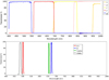 |
Fig. B.1 Profiles of the g′, r′, i′, z′, Y, Hß, OIII, Hα, and SII filters described in Table B.1. |
| In the text | |
|
Fig. C.1 Theoretical spectral resolving power of MISTRAL. The data for the blue and red configurations are from Table C.1. Top panel: Resolving power vs. wavelength. The straight lines are the linear fitting of these data. Bottom panel: FWHM vs. wavelength. The curves are computed from the linear fits. For comparison, the wavelength separation of several close stellar emission lines is marked with a diamond (resolved with MISTRAL) and crosses (unresolved with MISTRAL). |
| In the text | |
|
Fig. D.1 Red configuration spectrum of the spectrophotometry standard Feige 15 with MISTRAL, obtained with an exposure of 600 s on the night of 8 December 2021 (no telluric correction). The flux error bars are plotted in gray. The vertical light-gray stripes indicate the atmospheric absorption bands of water and molecular oxygen (Lu et al. 2021). The reference flux and bandwidth wavelengths are marked in red (Stone 1977, shortward of 8370 Å). The solid and dotted blue lines are the α Lyrae (Vega) CALSPEC spectrum and continuum (Bohlin et al. 2014), respectively, normalized at the wavelength and flux marked by the green plus. |
| In the text | |
|
Fig. F.1 Variation over time (starting at the Julian Date of 2459310) of the mean ADU level (top panel) and of the 1er mean level of the uncertainty (bottom panel) of the MISTRAL biases. |
| In the text | |
|
Fig. F.2 Variation over time (starting at the Julian Date of 2459310) of the mean ADU level (top panel) of the arc exposures of MISTRAL. The bottom panel shows the percentage of potential low-response pixels over time. |
| In the text | |
Current usage metrics show cumulative count of Article Views (full-text article views including HTML views, PDF and ePub downloads, according to the available data) and Abstracts Views on Vision4Press platform.
Data correspond to usage on the plateform after 2015. The current usage metrics is available 48-96 hours after online publication and is updated daily on week days.
Initial download of the metrics may take a while.