| Issue |
A&A
Volume 687, July 2024
|
|
|---|---|---|
| Article Number | A67 | |
| Number of page(s) | 14 | |
| Section | Extragalactic astronomy | |
| DOI | https://doi.org/10.1051/0004-6361/202347087 | |
| Published online | 27 June 2024 | |
JADES
Possible Population III signatures at z = 10.6 in the halo of GN-z11
1
Kavli Institute for Cosmology, University of Cambridge, Madingley Road, Cambridge CB3 0HA, UK
e-mail: This email address is being protected from spambots. You need JavaScript enabled to view it.
2
Cavendish Laboratory, University of Cambridge, 19 JJ Thomson Avenue, Cambridge CB3 0HE, UK
3
Department of Physics and Astronomy, University College London, Gower Street, London WC1E 6BT, UK
4
Centro de Astrobiología (CAB), CSIC-INTA, Cra. de Ajalvir Km. 4, 28850 Torrejón de Ardoz, Madrid, Spain
5
Institute of Astronomy, University of Cambridge, Madingley Road, Cambridge CB3 0HA, UK
6
Scuola Normale Superiore, Piazza dei Cavalieri 7, 56126 Pisa, Italy
7
National Astronomical Observatory of Japan, 2-21-1 Osawa, Mitaka, Tokyo 181-8588, Japan
8
Center for Astrophysics – Harvard & Smithsonian, 60 Garden St., Cambridge, MA 02138, USA
9
Department of Physics, University of Oxford, Denys Wilkinson Building, Keble Road, Oxford OX1 3RH, UK
10
Sorbonne Université, CNRS, UMR 7095, Institut d’Astrophysique de Paris, 98 bis bd Arago, 75014 Paris, France
11
INAF – Osservatorio Astrofisco di Arcetri, largo E. Fermi 5, 50127 Firenze, Italy
12
European Southern Observatory, Karl-Schwarzschild-Strasse 2, 85748 Garching, Germany
13
Centre for Astrophysics Research, Department of Physics, Astronomy and Mathematics, University of Hertfordshire, Hatfield AL10 9AB, UK
14
Max-Planck-Institut für Astronomie, Königstuhl 17, 69117 Heidelberg, Germany
15
Steward Observatory University of Arizona, 933 N. Cherry Avenue, Tucson, AZ 85721, USA
16
AURA for European Space Agency, Space Telescope Science Institute, 3700 San Martin Drive, Baltimore, MD 21210, USA
17
Department of Astronomy, University of Wisconsin-Madison, 475 N. Charter St., Madison, WI 53706, USA
18
Department for Astrophysical and Planetary Science, University of Colorado, Boulder, CO 80309, USA
19
Department of Astronomy and Astrophysics, University of California, Santa Cruz, 1156 High Street, Santa Cruz, CA 95064, USA
20
Astrophysics Research Institute, Liverpool John Moores University, 146 Brownlow Hill, Liverpool L3 5RF, UK
21
NSF’s National Optical-Infrared Astronomy Research Laboratory, 950 North Cherry Avenue, Tucson, AZ 85719, USA
Received:
3
June
2023
Accepted:
20
February
2024
Abstract
Finding the first generation of stars formed out of pristine gas in the early Universe, known as Population III (PopIII) stars, is one of the most important goals of modern astrophysics. Recent models have suggested that PopIII stars may form in pockets of pristine gas in the halo of more evolved galaxies. We present NIRSpec integral field spectroscopy and micro-shutter array spectroscopic observations of the region around GN-z11, an exceptionally luminous galaxy at z = 10.6, that reveal a greater than 5σ detection of a feature consistent with being HeIIλ1640 emission at the redshift of GN-z11. The very high equivalent width of the putative HeII emission in this clump (log(EWrest(HeII)/Å) = 1.79−0.25+0.15) and a lack of metal lines can be explained in terms of photoionisation by PopIII stars, while photoionisation by PopII stars is inconsistent with the data. The high equivalent width would also indicate that the putative PopIII stars likely have an initial mass function with an upper cutoff reaching at least 500 M⊙. The PopIII bolometric luminosity inferred from the HeII line would be ∼7 × 10⁹ L⊙, which would imply a total stellar mass formed in the burst of ∼2 × 10⁵ M⊙. We find that photoionisation by the active galactic nucleus (AGN) in GN-z11 cannot account for the HeII luminosity observed in the clump but can potentially be responsible for an additional HeII emission observed closer to GN-z11. We also consider the possibility of in situ photoionisation by an accreting direct collapse black hole hosted by the HeII clump. We find that this scenario is less favoured, but it remains a possible alternative interpretation. We also report the detection of a Lyα halo stemming out of GN-z11 and extending out to ∼2 kpc as well as resolved funnel-shaped CIII emission likely tracing the ionisation cone of the AGN.
Key words: stars: Population II / stars: Population III / galaxies: active / galaxies: high-redshift / galaxies: individual: GN-z11 / dark ages, reionization, first stars
© The Authors 2024
 Open Access article, published by EDP Sciences, under the terms of the Creative Commons Attribution License (https://creativecommons.org/licenses/by/4.0), which permits unrestricted use, distribution, and reproduction in any medium, provided the original work is properly cited.
This article is published in open access under the Subscribe to Open model. This email address is being protected from spambots. You need JavaScript enabled to view it. to support open access publication.
1. Introduction
The formation of the first stars and galaxies marks a fundamental transitional phase in cosmic history, during which the Universe evolved from a relatively simple state into the highly structured system we observe today (Bromm & Larson 2004). Almost all baryonic matter formed after the Big Bang, and the ‘dark ages’ were composed of hydrogen and helium. Consequently, the very first stars to form must have condensed out of these elements, primarily as a result of cooling due to the small amounts of H2 that could form at such early epochs (e.g. Kashlinsky & Rees 1983). These stars, called Population III (PopIII), are potentially very massive, up to several 100 M⊙, as a consequence of inefficient gas cooling and hence poor fragmentation of pre-stellar cores at these early epochs (e.g. Bromm et al. 1999; Abel et al. 2002; Tan & McKee 2004; Hirano et al. 2014; Susa et al. 2014). Indirect studies of Pop III stars via stellar archaeology have confirmed these predictions, suggesting that their masses extend up to 1000 M⊙, with a characteristic mass greater than 1 M⊙ (Rossi et al. 2021; Pagnini et al. 2023). Such massive PopIII stars are expected to be very hot and lead to an energetic photoionising spectrum capable of doubly ionising helium. Indeed, an expected signature of PopIII stars is prominent HeII nebular lines with very large equivalent widths (EWs; (HeIIλ1640)> 20 Å) unaccompanied by metal lines (Tumlinson & Shull 2000; Oh et al. 2001; Tumlinson et al. 2001; Schaerer 2003; Nakajima & Maiolino 2022). However, other models have also predicted that primordial gas might fragment more efficiently, resulting in the formation of cooler and less massive stars (e.g. Clark et al. 2011; Greif et al. 2011, 2012; Stacy et al. 2016).
While observations have found potential chemical fingerprints of the enrichment produced by the first generation of stars (Beers & Christlieb 2005; Frebel et al. 2007; Cooke et al. 2011; Hartwig et al. 2015, 2018; Salvadori et al. 2023; Saccardi et al. 2023; Klessen & Glover 2023; D’Eugenio et al. 2024; Christensen et al. 2023), PopIII stars in early galaxies have eluded detection so far, with some claims not being confirmed by subsequent studies (Sobral et al. 2015, Bowler et al. 2017, Harikane et al. 2018). However, the unprecedented sensitivity of JWST is pushing the frontier of observations to high redshift and very faint galaxies, discovering very low metallicity systems (Vanzella et al. 2023) and indicating that the detection of PopIII stars may be within reach of this observatory (see also e.g. Zackrisson et al. 2011).
Further encouraging expectations about the detectability of PopIII stars have been obtained by recent cosmological simulations. Indeed, two main formation phases of PopIII stars have been proposed. Firstly, PopIII stars could have formed in dark matter mini halos at redshifts z ∼ 10–30 (e.g. Tegmark et al. 1997; Bromm et al. 2009; Pallottini et al. 2014; Jeon et al. 2015, Maio et al. 2009, 2010; Vikaeus et al. 2022; Ventura et al. 2023; Trinca et al. 2024). Secondly, PopIII stars could still have formed at later times, down to redshifts of about z ∼ 3–6, in pristine or low-metallicity pockets of gas due to the highly inhomogeneous nature of metal enrichment in the Universe, as well as a consequence of re-accretion of pristine gas (e.g. Tornatore et al. 2007; Johnson 2010; Liu & Bromm 2020, Sarmento et al. 2018; Jaacks et al. 2019, Katz et al. 2023, Volonteri et al. 2023). In these cases, PopIII stars are expected to be found in the halos of more massive galaxies, and their hard ionising spectrum may be ionising mildly enriched gas, resulting in weak emission of metal lines (Nakajima & Maiolino 2022; Katz et al. 2023; Jaacks et al. 2018).
Although PopIII stars are expected to be present even at relatively low redshifts (possibly down to z ∼ 3; Cassata et al. 2013; Liu & Bromm 2020) in the latter scenario, the probability for a halo to host PopIII stars is higher at very high redshift (Trinca et al. 2023). Within this context, GN-z11 is an exceptional galaxy at z = 10.6, as it offers an optimal environment to search for PopIII stars. Identified initially by Bouwens et al. (2010) and Oesch et al. (2016), GN-z11 is the most luminous galaxy at z > 10 in all Hubble Space Telescope (HST) fields (including all fields in the Cosmic Assembly Near-infrared Deep Extragalactic Legacy Survey, CANDELS, and all Frontier Fields, Oesch et al. 2018). Recent JWST-NIRCam imaging from the JWST Advanced Deep Extragalactic Survey (JADES, Eisenstein et al. 2023) has revealed that GN-z11 is characterised by an unresolved central source, a more extended component (200 pc in radius) with Sérsic index n = 1, and a more diffuse component extending for ∼0.5″ to the NE (the ‘haze’), which may not be associated with GN-z11 and could simply be a foreground system (Tacchella et al. 2023). Bunker et al. (2023) obtained low- and medium-resolution spectroscopy of GN-z11 with JWST-NIRSpec in the multi-object spectroscopy (MOS) mode using the micro-shutter assembly (MSA), revealing a spectrum with a wealth of nebular emission lines in various ionisation stages and characterised by some unusual line ratios. Interestingly, the spectrum revealed Lyα emission extended along the slit for about 0.2″ (∼0.8 kpc) towards the SW (the position angle of the shutter was 19.9°). Additional NIRSpec MSA observations targeting GN-z11 have led to the identification of an active galactic nucleus (AGN) in GN-z11 (Maiolino et al. 2024), primarily through the detection of high ionisation lines (NeIV), semi-forbidden lines tracing very high densities consistent with the broad-line regions of AGNs, and the detection of the CII*λ1335 fluorescent emission, typically seen only in AGN. The spectrum of GN-z11 has also revealed the presence of a powerful outflow traced by the redshifted (∼530 km s−1) and resonantly scattered emission of both Lyα and CIVλ1550 and the blueshifted absorption of CIV (∼800 − 1000 km s−1). The second NIRSpec MSA observation had a position angle nearly perpendicular to the first observation and did not show obvious evidence for Lyα extension on either side of GN-z11.
A more detailed analysis of the 2D spectrum of GN-z11 in the first observation has revealed the tentative emission of a line located at ∼0.5″ to the NE of GN-z11 at a wavelength consistent with HeIIλ1640 at the same redshift of GN-z11 (see Sect. 3.1). This intriguing finding prompted a DDT proposal to obtain NIRSpec integral field unit (IFU) spectroscopy of GN-z11 with both the G140M (3.3 h) and G235M (10.6 h) gratings. The IFU datasets deliver superior spatial information relative to the MSA (although the sensitivity is lower than the MSA because the IFU has an about 50% lower throughput).
In this paper we report a preliminary analysis of the new NIRSpec-IFU data of GN-z11 that confirm the HeIIλ1640 detection at z = 10.6 as well as additional interesting features associated with the Lyα and CIII] morphology. Throughout this work, we use the AB magnitude system and assume a Planck flat ΛCDM cosmology with Ωm = 0.315 and H0 = 67.4 km s−1 Mpc−1 (Planck Collaboration VI 2020). With this cosmology, 1″ corresponds to a transverse distance of 4.08 proper kpc at z = 10.6.
2. Observations, data processing, and data analysis
GN-z11 was observed with NIRSpec-IFU (Jakobsen et al. 2022; Böker et al. 2022) on 22 to 23 May 2023 under the DDT programme 4426 (PI: Roberto Maiolino). The observational setup utilised a medium cycling pattern of 10 dithers for a total integration time on source of 10.6 h with the medium-resolution grating-filter pair G235M/F170LP, and 3.3 h with the medium-resolution grating-filter pair G140M/F100LP. These configurations cover the spectral ranges of 0.97–1.89 and 1.66–3.17 μm, with a nominal spectral resolution of R ∼ 1000. The detector was set with the improved reference sampling and subtraction pattern (IRS2), which significantly reduces the read out noise with respect to the conventional method (Rauscher et al. 2012). We also checked that no bright foreground sources were at the location of the MSA quadrants, where they could significantly contaminate the IFS spectra.
Although JWST has an excellent pointing accuracy (i.e. 0.1″, 1σ radial1Rigby et al. 2023), and the telescope was commanded to the location of GN-z11 provided by the NIRCam and HST imaging and Gaia-referenced astrometry, the observations were affected by a guiding problem of the observatory because the guide star turned out to be a binary (report from the Fine Guidance Sensor team). This introduced a large offset of about 1.4″ towards the SE. This offset located GN-z11 as being close to the edge of the IFU field of view (FoV). This restricted the zone around GN-z11 that could be explored, lowering the S/N of regions that were covered by fewer dither positions or excluding completely some regions from the FoV. More specifically, out of the 10 dither positions, GN-z11 itself was located right at the edge of the FoV in three of them, and in another four of them GN-z11 was so close to the edge that the SW extension of the Lyα was mostly outside the FoV. As we attempt an analysis of the SW extension based on the incomplete data in this paper, our work on that regard will need to be validated by planned future observations that will repeat the dithers that were more severely affected (within the context of the same programme 4426). As a consequence, the main focus of this paper is on the extended emission towards the NE.
Because of the guiding problem, the world coordinates given by the pipeline in the header of the final IFU cube are off by about 1.4″. Therefore, we corrected the world coordinates by realigning the cube to the NIRCam image by collapsing the cube in the same band as in the NIRCam filter (although the centroid of the continuum does not change with wavelength).
Raw data files were downloaded from the MAST archive and subsequently processed with the JWST Science Calibration pipeline2 version 1.8.2 under CRDS context jwst_1068.pmap. We made several modifications to the default reduction steps to increase the data quality, which are described in detail by Perna et al. (2023) and which we briefly summarise here. The default pipeline is occasionally subject to over-subtraction of elongated cosmic ray artefacts through the default circular correction applied to ‘snowball-like’ cosmic ray hits. To avoid this problem, we patched the pipeline to fit ellipses to all flagged regions consisting of five or more adjacent pixels. The regions with best-fit ellipses with axial ratios smaller than 0.1 were removed from the list of ‘snowball-like’ cosmic rays. Count rate frames were corrected for 1/f noise through a polynomial fit. Outliers were flagged on the individual 2D exposures using an edge-detection algorithm similar to LACOSMIC (van Dokkum 2001). We calculated the derivative of the count rate maps along the x-axis of the detector (on the scale of a few pixels, the x-axis is a good approximation for the dispersion direction). The derivative was normalised by the local flux (or by three times the rms noise, whichever was highest), and we rejected the 95th percentile of the resulting distribution – the percentiles were calculated over the entire detector area (see D’Eugenio et al. 2023, for details). In addition, we made the following corrections to the *cal.fits files after Stage 2: We masked pixels at the edge of the slices (two pixels wide) to conservatively exclude pixels with unreliable sflat corrections. We also masked regions affected by leakage from failed open MSA shutters. We note that the data quality flag ‘MSA_FAILED_OPEN’ fails to account for all failed open MSA shutters. At the same time, several regions marked as being affected by failed open shutters do not show any impact from leakage, and we included those regions to increase S/N in the final combined cube. Finally, we masked regions that were affected by persistence in all dither frames (e.g. from cosmic rays). The final cubes were combined using the ‘drizzle’ method with pixel scales of 0.06″ and 0.10″, for which we used an official patch to correct for a known bug3.
We also re-analysed the NIRSpec-MOS observations of GN-z11 obtained in February 2023 within the JADES survey but with a focus on the 2D extraction along the shutters. These observations were described in Bunker et al. (2023). Here, we only remind that those observations were obtained with four configurations of the MSA (Jakobsen et al. 2022; Ferruit et al. 2022; Böker et al. 2023), each with three shutters nodding. The low-resolution prism and the three medium-resolution gratings were used, for a total observing time of 6.9 h with the prism and 3.45 h with each of the gratings. In the following, to explore the 2D information we use only the prism, as the gratings exposures are shallower. The processing of the MSA data is also described in Bunker et al. (2023); here, we only recall that we have used the pipeline developed by the ESA NIRSpec Science Operations Team and the NIRSpec GTO Team. We also recall that the spatial pixel size in the MSA 2D spectra is 0.1″ and that each shutter is 0.2″ wide. The standard background subtraction method does not allow for exploration of the extended emission along the shutters. Indeed, the nodding technique moves the target by one shutter position (i.e. by 0 53) along the shutter’s direction. When reciprocally subtracting two exposures in which the source is located in adjacent shutters, this results in a deep negative trace of the subtracted source spectrum at ±0.5″ from the (positive) spectrum of the source and at least as wide as the PSF and its wings (∼0.2″), depending on the source size. This makes the standard 2D spectrum unusable in the exploration of any extended emission beyond ∼0.2″ from the source. Therefore, in order to explore the 2D information along the shutter and avoid self-subtraction of the extended emission, we used a different background subtraction process relative to standard process adopted in Bunker et al. (2023). Specifically, we did not use the exposure with the source in the central shutter. Instead, we used only the exposures in which the source is in the upper and lower shutters (i.e. the exposures with the source in the most distant positions) to perform mutual background subtraction. This ensured that the subtracted negative traces of the GN-z11 spectrum are located at ∼1″ from the (positive) spectrum and enabled the study of spectral features along the shutter up to about 0.6″ from the source. This method obviously slightly reduces the sensitivity of the data, as we only used two-thirds of the data, and the noise in the background was increased by a factor of
  , but it is far superior relative to the standard method for exploring extended emission.
The tilted boxes in Fig. 1 show the footprint of the shutters in the four MSA configurations of the MOS observation from February 2023 overlaid on the F277W image of GN-z11 (Tacchella et al. 2023). The white circle indicates the target acquisition uncertainty of the MSA, meaning that the footprints indicated in the figure may actually be displaced in any direction by that amount. The orange vertical dashed line indicates the region beyond which fewer exposures from the NIRSpec-IFU DDT programme are available (and with GN-z11 at the edge of the field of view) because of the telescope guiding problem discussed above.
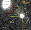 |
Fig. 1. F277W NIRCam image of the central ∼1.7″ around GN-z11 illustrating the location of the MSA shutters during the first NIRSpec-MOS observations in February 2023 (tilted boxes; boxes of the same colour are associated with the same configuration), the extraction region of the HeII clump (red square), and the HeII extended emission (yellow box). The white circle indicates the absolute uncertainty of the MSA target acquisition (hence the shutters’ footprints are uncertain by this amount). North is up, and east is to the left. The orange vertical dashed line marks the boundary beyond which fewer dithers from the NIRSpec-IFU observations are available because of the guiding problem reported in Sect. 2. We note that the full IFU FoV is larger than shown here (> 3″ × 3″ taking into account the dithers). |
When extracting spectra and emission line maps, we removed background and continuum emission with the following procedure: We extracted the background from an area of the IFU free from artefacts and performed sigma-clipping of the outliers. The resulting spectrum was smoothed with a rolling median of 25 spectral pixels. This background was normalised to the continuum in the vicinity of the spectral feature and subtracted. Since the background has some residual structure across the IFU FoV, also because of the possible continuum contribution from individual sources (especially in the case of GN-z11), we further optimised the continuum subtraction by linearly interpolating the continuum within a range of a few 0.01 μm around the line of interest after masking the emission line (typically within ±3 spectral pixels from the line peak). In the case of the Lyα, the latter step could be more problematic on GN-z11, as the galaxy continuum is asymmetric relative to Lyα due to the intergalactic medium (IGM) absorption (which also affects the continuum red-wards of the Lyα because of the damping wing). However, we were primarily interested in the extended emission where the galaxy continuum is not detected. However, we also explored the subtraction of the continuum around Lyα by fitting the continuum only on the red side of the line, and the result did not change, except for a slight increase in the noise on the extended component, as expected from the poorer sampling of the background.
3. Results
3.1. HeII detection in the halo of GN-z11
We start by illustrating the tentative detection of HeIIλ1640 in the 2D spectrum along the shutters in the NIRSpec MSA observation of February 2023. We show the S/N 2D spectrum of GN-z11 in the top panel of Fig. 2. As already discussed, this was reprocessed to use only the exposures in which GN-z11 is in the upper and lower shutters (hence discarding the exposure with GN-z11 in the central shutter) in order to prevent self-subtraction of extended emission. The 2D spectrum shows a tentative signal at 1.905 μm, which is consistent with the expected location of HeIIλ1640 at the redshift of GN-z11 (z = 10.603), peaking at about 0.5″ from GN-z11. The bottom panel shows the spectrum extracted from the region of the 2D spectrum delimited by the two horizontal dashed lines in the upper panel. The black dotted line indicates the noise level per spectral pixel. The extracted spectrum confirms the emission feature at 1.905 μm. The integrated significance of the feature is 3.7σ, as reported in Table 1. We note that this feature is totally impossible to detect with the standard background subtraction procedure adopted in Bunker et al. (2023), because in that case the deep negative trace of the GN-z11 subtracted spectrum falls exactly at this location. This is the first negative trace, next to the (positive) spectrum of GN-z11, in the top panel of Fig. 1 of Bunker et al. (2023). With our method, we avoided the negative traces nearest the GN-z11 spectrum (i.e. those at ±0.5″ from the spectrum of GN-z11 in the 2D spectrum of Bunker et al. 2023). We also note that the absolute flux and spatial centroid of the feature are affected by some additional uncertainty associated with the 2D extraction. Specifically, the feature is at the edge of the region beyond which self-subtraction can still happen, even when adopting our two-shutter methodology. This can result in both flux uncertainty and the centroid being slightly artificially shifted towards GN-z11. Secondly, in some exposures, the feature falls next to or beneath the shutter bar (see Fig. 1). This can also affect the flux and centroid. Finally, the aperture losses applied to the spectrum are based on the point-like assumption and on using the location of GN-z11 (which is next to the bar or to the slit edge in some exposures). Hence, these corrections may result in additional flux uncertainties when applied to the putative HeII feature, which is located in another region of the shutters.
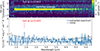 |
Fig. 2. Prism spectrum of the region to the north-east of GN-z11, from the February 2023 MSA observation. Top panel: signal-to-noise 2D prism spectrum of GN-z11. The spectrum has been obtained by using only the exposures in which GN-z11 is in the upper and lower shutters (hence discarding the exposure with GN-z11 in the central shutter) as to avoid self-subtraction of the extended signal. Bottom panel: one-dimensional spectrum extracted from the region delimited by the two dashed horizontal lines, at about 0.45″ from GN-z11 in the NE direction, illustrating the tentative detection (3.7σ integrated) of a feature at 1.903 μm. The red vertical line indicates the location of HeIIλ1640 expected at the redshift of GN-z11, z = 10.603 (which is indistinguishable from the redshift of 10.600 inferred for the grating spectrum). |
Measured fluxes, EWs, and 3σ limits in the apertures considered in this paper.
Figure 3 shows the maps at the expected wavelengths of HeII, Lyα, and CIII] obtained from the NIRSpec-IFU observation. Specifically, HeII was extracted from 1.9003 μm to 1.9035 μm, CIII] from 2.2099 μm to 2.2173 μm, and Lyα from 1.4115 μm to 1.4152 μm. The extraction of CIII] and Lyα is on a slightly broader range, as the former is a doublet (hence, it is slightly broader, although still unresolved at our resolution), and Lyα has a broad profile. We note that the Lyα map has been centred on the Lyα offset observed in GN-z11 (−550 km s−1). The maps have also been slightly smoothed with a Gaussian kernel with a width of 1.5 pixels (0.09″).
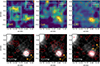 |
Fig. 3. Emission lines maps. Top panels: maps of the HeIIλ1640, Lyα, and CIII]λ1909 lines (see text for details). The red star marks the position of the continuum of GN-z11. Contours are at 2, 3, and 4σ for the HeII and Lyα maps and at 2, 4, 6, and 8σ for the CIII] map (the rms is estimated from the statistics in the IFU FoV, outside this region). We note that most of these spaxels are independent; hence the significance of the integrated emission of each feature is significantly higher. The two white boxes indicate the extraction apertures of the two spectra shown in Fig. 4 and marked in red and yellow in Fig. 1. The vertical dashed segment indicates the region beyond which there are fewer exposures because of the guiding problem discussed in Sect. 2. Bottom panels: overlay of the contours from the emission line maps onto the F277W NIRCam map from Tacchella et al. (2023). |
Since the emission features are extended, the significance of the integrated emission of the individual clumps is higher than that given by the contours. The HeII map shows a plume extending for about 0.25″ towards the west of GN-z11 (red star). This is the area with fewer exposures (due to the guiding problem), so it should be treated with great care. Yet, if it is confirmed, such a HeII plume would extend well beyond the size of the galaxy identified by Tacchella et al. (2023) and may be tracing gas photoionised by the AGN. The weak CIII] at this location (and the fact that no CIV emission is seen either) would indicate that this is very low metallicity gas photoionised by the AGN.
The most intriguing feature in Fig. 3 is the clump located at about 0.6″ (2.4 kpc) to the NE. This is very close to the location of the emission serendipitously found along the shutter of the MSA prism observation (Fig. 2), especially when also taking into account the MSA target acquisition uncertainty and the fact that the MSA observation still suffers signal self-subtraction at locations farther than 0.5″ from GN-z11 (as well the additional uncertainties discussed in the previous section). We extracted the spectrum from this region by taking a 0.24″ × 0.24″ square aperture (red box in Fig. 1; ‘HeII clump extraction’, smaller white box in Fig. 3; and Table 2). The resulting spectrum is shown in the top-left panel of Fig. 4, which shows the detection of a line at λobs = 1.902 μm whose integrated significance is 5.5σ (Table 1). This corresponds to the wavelength of HeIIλ1640 at a redshift of 10.600, fully consistent with the redshift of GN-z11.
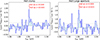 |
Fig. 4. Spectra extracted from the apertures indicated in Fig. 1 and zoomed near the expected wavelength of HeII at the redshift of GN-z11. Specifically, the left panel shows the spectrum extracted from the aperture centred on the ‘HeII clump’ (red box in Fig. 1 and smaller white box in Fig. 3). The right panel shows the spectrum extracted from the larger aperture encompassing the extended HeII emission in the NE quadrant of GN-z11 (yellow box in Fig. 1 and larger white box in Fig. 3). The red vertical bars indicate the expected wavelength of HeII at the redshift of GN-z11, z = 10.603, and the wavelength of the centroid of the line in the clump, which, if identified as HeII, gives a redshift z = 10.600. The dotted lines indicate the noise per spectral pixel in each spectrum inferred from the rms directly measured in the spectrum around the HeII line. |
Extraction apertures.
It is unlikely that this feature is Hα or [OIII]λ5007 of a lower redshift interloper, specifically at z = 1.90 or z = 2.80, as other bright lines expected at these redshifts are not seen. The ‘haze’ identified in imaging by Tacchella et al. (2023) is probably a lower redshift interloper, but it is offset (closer to GN-z11) relative to the putative HeII clump. We indeed identified an emission line at 2.330 μm peaking on the ‘haze’ that we tentatively identify as [OIII] at z = 3.65 (see Appendix B for details), consistent with the photometric redshift inferred by Tacchella et al. (2023). The large foreground galaxy at z = 2.028 to the NE of the clump does not have any line emission at this wavelength (see spectrum in Appendix B), and any weak emission feature potentially associated with that galaxy would also show a much stronger Hα associated with it, as well as many other stronger emission lines.
We also explored whether some Lyα emission is leaking out of the intergalactic medium (IGM) absorption at this location. We found a tentative detection of Lyα, but it requires additional data for confirmation. Therefore, we do not discuss this any further.
It is difficult to compare the fluxes of the putative HeII seen in the IFU clump and the detection in the MSA. In terms of wavelength, they are fully consistent. In terms of flux, it is more difficult. At face value, the fluxes reported in Table 1 give a higher flux in the MSA (with a large error). However, because of the uncertainty on the exact location of the MSA shutter (see Sect. 2 and white circle in Fig. 1), the actual fraction of the putative HeII clump that entered the shutters is not known. Moreover, the potential absolute flux calibration issues plaguing the MSA at the location of the putative HeII mession, as discussed above, introduce additional uncertainties that prevent a proper comparison. Finally, we note that the MSA prism observation is more sensitive than the IFU observation (as discussed in Sect. 1). Hence, it may be detecting additional HeII emission outside the clump not seen in the IFU cube. Additionally, faint emission at slightly different velocities (as discussed in Appendix B) may be missed by the higher resolution of the grating, but picked by the much broader line spread function of the prism.
In addition to the clump at ∼0.6″ to the NE from GN-z11, the HeII emission appears to have additional and more extended emission, as seen in the map in Fig. 3 (top left panel), mostly distributed in the NE quadrant of GN-z11, possibly with a fainter and less significant clump about 0.3″ south of the HeII primary clump and about 0.4″ east of GN-z11. We extracted the spectrum from this larger area by using the large aperture marked with the yellow box in Fig. 1 (larger white box in Fig. 3). The resulting spectrum at the wavelength of HeII at z = 10.600 is shown in the right panel of Fig. 4. In this case, the putative HeII emission is detected at 6.1σ and with a total flux that is about two times higher than in the clump. We note that the putative HeII emission detected in this larger aperture is certainly not polluted by HeII emission in GN-z11. To begin with, the HeII emission of GN-z11 is very faint (Maiolino et al. 2024; Bunker et al. 2023); contamination by GN-z11 would imply that all other strong lines seen in GN-z11 would be detected and would be much brighter than HeII. Secondly, as shown in Appendix C, we also extracted a spectrum by modifying this large aperture in order to remove the region closer than 0.3″ (more than six times the PSF radius at this wavelength) from GN-z11, and the detection remained unchanged (Fig. C.1), therefore confirming that the weak HeII emission from GN-z11 does not contribute at all to the spectrum extracted in this region.
3.2. Lyα halo and morphology
Although not the focus of this paper, in the middle panel of Fig. 3, we also show the map of the Lyα emission. Here, we have simply collapsed the background- and continuum-subtracted channels around the redshifted peak observed in GN-z11 (Sect. 3.1). A more in-depth analysis of the full Lyα profile will be presented in a forthcoming paper. The Lyα emission is clearly extended, partly in the western direction relative to GN-z11 (red star) but mostly towards the SW, as expected from the MOS data when taken along this orientation (Bunker et al. 2023). The extension towards the SW is very sharp and could potentially trace an accreting filament. However, as discussed in the next section, the fact that we also see lopsided CIII] emission in this direction favours the interpretation that the emission in the SW stems from gas illuminated in the ionisation cone of the AGN in GN-z11. We, however, warn that this region falls in the area with less exposure because of the telescope guiding problem discussed in Sect. 2, so the emission in this region could potentially extend farther to the SW. A proper investigation requires additional data that will be obtained in the repeated observations.
At a low surface brightness level, Lyα extends smoothly and over a larger area also towards the north, with a peak at about 0.4″ to the NE of GN-z11. The nature of the extended Lyα emission will be discussed more extensively in a dedicated paper.
3.3. CIII] extension and the ionisation cone
The CIII]1909 doublet is one of the brightest metal lines observed in the spectrum of GN-z11, and it is the only metal line of GN-z11 that is clearly resolved in the IFU observations. Its continuum-subtracted map is shown in the right panel of Fig. 3. The CIII] emission is clearly elongated in the NE-SW direction and most prominently extended towards the SW, with a funnel-shaped geometry. We note that the elongation is not an artefact of the data processing, as we demonstrate in the Appendix (where we compare it with the continuum map extracted around the same wavelength). The most plausible interpretation is that this emission is tracing the ionisation cone of the AGN in GN-z11. Although no CIV was clearly detected in this region (which however might be self-absorbed; Maiolino et al. 2024), the emission line properties are fully consistent with an AGN photoionisation scenario with a low ionisation parameter, likely due to the distance from the AGN (Feltre et al. 2016; Nakajima & Maiolino 2022). Once again, since this extended emission falls in the region where the exposure time is shorter, because of the telescope guiding problem discussed above, the investigation of this extended emission therefore requires the additional data that will be obtained in the repeated observations.
4. The case for pristine gas and Population III
As discussed in Sect. 3.1, the most likely identification of the emission line observed at 1.902 μm in the halo of GN-z11 is the HeIIλ1640 emission at z = 10.600. In the vicinity of GN-z11, specifically the western plume and some of the extended emission towards the NE quadrant, the HeII emission may likely trace gas photoionised by the AGN in GN-z11. The fact that no or little emission from metal lines (in particular CIV, CIII], and OIII]) was detected in these regions suggests that such circumgalactic gas has a low metallicity. However, it is also possible that the low intensity of all metal lines is a consequence of the low ionisation parameter (Feltre et al. 2016; Nakajima & Maiolino 2022). Yet, empirically, when extended HeII emission is observed in other halos surrounding AGNs at lower redshift, this is always accompanied by even brighter CIV emission and possibly CIII] emission (Guo et al. 2020; Fossati et al. 2021). Therefore, the finding of extended HeII emission around an AGN at z > 10 not accompanied by CIV emission suggests that this is primarily due to much lower gas metallicity in the halo.
Although the gas closer to GN-z11 may be photoionised by the AGN, the HeII emission seen in the NE clump at ∼0.6″ (2.4 kpc) from GN-z11 cannot be explained in terms of photoionisation by the AGN simply based on ionising photon budget arguments. Indeed, HeIIλ1640 is a simple recombination line that is essentially a counter of photons more energetic than 54 eV from the impinging radiation. As a consequence, by knowing the luminosity of the AGN (Maiolino et al. 2024) as well as the distance and size of the cloud (or its upper limit), one can estimate the number of HeI ionising photons reaching the cloud and the resulting HeII luminosity. We assumed a broad range of AGN ionising spectra (Nakajima & Maiolino 2022) and that the observed projected distance gives the actual distance of the clump to GN-z11. This obviously is a conservative assumption, as the actual distance is larger and results in a lower flux of ionising photons. We also assumed that within the clump, the covering factor of the absorbing gas is unity. In other words, we have made the additional conservative assumption that the gas in the cloud is not ‘clumpy’, and hence all radiation reaching it is fully absorbed. The result of this calculation is shown in Fig. 5, where the blue shaded area shows the expected HeII luminosity as a function of distance from GN-z11, assuming photoionisation by the AGN in GN-z11 and by adopting all AGN ionising continuum shapes considered in Nakajima & Maiolino (2022). We also assumed isotropic emission, which is another conservative assumption given that the AGN in GN-z11 is type 1 (Maiolino et al. 2024). The luminosity observed in the HeII clump (L(HeII) = 2.8 × 1041 erg s−1, based on the flux reported in Table 1)4 is shown with the golden symbol, which is clearly inconsistent with AGN photoionisation by more than one order of magnitude, even ignoring that all assumptions made are very conservative. We note that we have assumed stable emission, but it is very unlikely that the luminosity of the AGN can change by two orders of magnitude because the variability observed so far is constrained to the level of 10% (Maiolino et al. 2024).
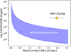 |
Fig. 5. Observed HeIIλ1640 luminosity of the ‘HeII clump’ and its projected distance from GN-z11 compared to the expected HeII luminosity as a function of distance from GN-z11, in case of AGN photoionisation. In this calculation, we used the upper limit for the size of the HeII clump and assumed a broad range of AGN ionising shapes powering the photoionisation. Further conservative assumptions are that the ‘HeII clump’ is not made of unresolved clumps and that the projected distance is the actual separation. Clearly, the HeII luminosity observed in the ‘HeII clump’ is inconsistent with being photoionised by the AGN in GN-z11. |
The HeII emission in the clump must therefore result from in situ photoionisation. In Fig. 6, we explore the source of ionising photons and gas metallicity by using diagnostic diagrams in which the EW of the HeII line is compared with various line ratios, specifically: HeII/Hγ, CIVλ1550/HeII, CIII]λ1909/HeII, and OIII]λ1665/HeII. We compared these quantities with the photoionisation models presented in Nakajima & Maiolino (2022). Specifically, the purple stars jn Fig. 6 illustrate the case of photoionisation by PopII stars (through metal-poor models from the BPASS libraries) with a broad range of ionisation parameters and densities and with (absolute) metallicities ranging from 10−5 to 10−3. In these models, the gas and stars are assumed to have the same metallicity. The blue symbols show the models for PopIII ionising continua. The dark blue circles are the case of PopIII embedded in pristine gas. The light blue squares and cyan triangles show the case of PopIII photoionising slightly enriched gas, as indicated in the legend. In the case of PopIII, Nakajima & Maiolino (2022) used a Salpeter IMF with three different stellar ranges: 1–100 M⊙, 1–500 M⊙, and 50–500 M⊙. In Fig. 6, these ranges are coded with PopIII symbols of different sizes, as indicated in the legend. We note that despite the high mass range explored in Nakajima & Maiolino (2022), a Salpeter IMF may not be appropriate for PopIII (e.g. de Bennassuti et al. 2014, 2017; Stacy et al. 2016; Venditti et al. 2023), and the EW(HeII) for PopIII may therefore have values even higher than those obtained by those models.
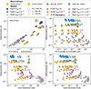 |
Fig. 6. Diagnostic diagrams showing the EW of HeIIλ1640 versus various line ratios: HeII/Hγ, CIVλ1550/HeII, CIII]1909/HeII, and OIII]λ1665/HeII. The observational constraints on the HeII clump in the halo of GN-z11 are shown with golden symbols, while the observational constraints for the HeII emission obtained from the large aperture extraction are shown with green symbols. Circles are for EWs for which the continuum has been inferred from photometry, while squares show the EWs for which the continuum constraints have been inferred directly from the spectra. Purple stars show PopII models with different (absolute) metallicities (colour-coded with different purple shadings) and where the gas and stars are assumed to have the same metallicity. Blue circles are models of PopIII stars in a pristine gas; light blue squares are models of PopIII stars in a mildly enriched gas, specifically Zgas = 10−5; light blue triangles are models of PopIII stars in a more enriched gas, specifically Zgas = 10−4. The PopIII markers have different sizes depending on the stellar mass range assumed for the IMF, as indicated in the legend. Orange pentagons show the predictions for accreting DCBHs embedded in gas with different (absolute) metallicities. |
The constraints on the HeII clump in the halo of GN-z11 are shown with golden symbols. The continuum is totally undetected in the IFS medium-resolution spectra and only marginally detected in the low-resolution prism MSA spectrum. Therefore, we primarily used the method adopted by various other studies of determining the continuum estimating the EW from the imaging photometry (e.g. Stark et al. 2017; De Barros et al. 2017; Mainali et al. 2018; Jung et al. 2020; Kusakabe et al. 2020; Boyett et al. 2022; Matthee et al. 2023). The constraints on the HeII clump using the continuum determination from photometry are shown with golden circles in Fig. 6. We note that the top-left diagram is only for the MSA prism measurement, as we needed a constraint on Hγ, while the other panels are for the IFU+grating measurements. We also provide (golden squares) the constraints obtained from the continuum non-detection in the IFS medium-resolution spectroscopic data as well as the estimation of the EW of the clump directly from the MSA low-resolution spectrum. A more detailed description of the derivation of the EW constraints is given in Appendix D. The resulting EWs are given in Table 1. The EW(HeII) inferred for the IFS spectrum of the clump and for the MSA spectrum are consistent with each other given the uncertainties.
For the HeII/Hγ ratio, we used the data from the prism, as Hγ is not covered by the new IFU observations. (We note that the HeII/Hγ is a lower limit, given that Hγ was not detected; see Table 1). In this case, we measured the EW consistently from the MSA prism spectrum, both by extracting the continuum from photometry at the corresponding aperture along the MSA shutter (golden circle) and by directly estimating the continuum from the spectrum (golden square), as reported in Table 2.
We also report the constraints on the HeII emission extracted from the larger aperture (green symbols). Although, as mentioned, in this case, part of the emission may be associated with the AGN photoionisation.
Figure 6 illustrates that the high EW(HeIIλ1640) observed in the HeII clump, specifically  from the IFU and
  from the MSA, is inconsistent by nearly two orders of magnitude with the PopII models but consistent with the PopIII models. Furthermore, it requires an IMF with a very large upper mass cutoff, about 500 M⊙. To explain the very large EW(HeII), an even higher stellar mass cutoff is possibly needed or an IMF more top-heavy than Salpeter in addition to the high mass cutoff or perhaps a log-flat IMF (Chon et al. 2021) is required.
We emphasise that in order to be consistent with the PopII models, the continuum flux of the clump should be about 80 nJy (i.e. nearly as strong as GN-z11), which is totally inconsistent with the data (Table 3) and therefore excludes the PopII scenario with a very high level of confidence. To make our point more clearly, we note that the 2σ lower limit on the EW(HeII) from the photometry method is 20 Å, which is totally inconsistent with the PopII scenario.
Continuum flux densities in HeII clump from NIRCam.
The lower limit on the HeII/Hγ ratio (Fig. 6, top left; see also Table 1) is consistent with the constraint from the EW(HeII), that is, requiring photoionisation from PopIII stars and possibly having an IMF with a very massive upper mass cutoff. In contrast, the upper limits from the metal lines (see Table 1) are not very constraining in terms of metallicity, and we cannot exclude that the PopIII stars are embedded in some moderately enriched gas, although the CIV/HeII upper limit is at the borderline with the models of PopIII living in a gas with a metallicity of 10−4.
By using the PopIII models with the massive upper cutoff IMFs (1–500 M⊙ and 50–500 M⊙), we inferred the ratio between HeII luminosity and total bolometric luminosity (∼10−2 for the two IMF models with the highest cutoff masses, which are better matches with the observations). This gave a bolometric luminosity of 2.7 × 1043 erg s−1 for the PopIII in the clump. Assuming an Eddington limited luminosity, this gave a mass of only 2 × 10⁵ M⊙. Alternatively, by using the ZAMS mass to luminosity conversions for PopIII given by Schaerer (2002), the inferred bolometric luminosity would give a total stellar mass of 2.5 × 10⁵ M⊙, similar to the value obtained above assuming an Eddington limited luminosity. These values for the total PopIII stellar mass are not far from the PopIII stellar mass expected from some recent simulations. Indeed, these simulations expect a halo hosting a PopII stellar mass similar to GN-z11 (∼8 × 10⁸ M⊙ in the extended component, Tacchella et al. 2023) to harbour a fractional mass of PopIII stars of about 3 × 10⁻⁴ − 1 × 10⁻³, that is, a total PopIII stellar mass of ∼2 − 8 × 10⁵ M⊙ (Yajima et al. 2023; Venditti et al. 2023; A. Venditti, priv. comm.).
It is worth noting that in addition to the extended HeII emission and although the map is noisy, the HeII clump itself seems resolved and possibly extended over ∼0.25″ (i.e. ∼1 kpc). This is much larger than the expected size of a single PopIII sub-halo, and it is much more likely that the extension is associated with a cluster of PopIII sub-halos. Indeed, according to recent simulations, PopIII sub-halos are expected to cluster in regions of a few kiloparsecs (Tornatore et al. 2007; Venditti et al. 2023). Alternatively, the extension may trace a large clump of pristine gas that is being photoionised by a single halo of PopIII stars embedded in it.
Finally, we also considered the possibility that the HeII clump is ionised in situ by an accreting direct collapse black hole (DCBH) seed in a pristine, or very low-metallicity, gas cloud. Nakajima & Maiolino (2022) have explored this case in their photoionisation calculations, and their models are shown with orange pentagons in Fig. 6. The darker orange symbols show the case of a DCBH photoionising pristine (zero metallicity) gas, while lighter shades of orange indicate the case of moderately enriched gas, as indicated in the legend. As for the PopII and PopIII cases shown in the same figure, the DCBH models explore a broad range of densities and ionisation parameters. Additionally, the models explore a broad range of plausible ionising shapes for the accreting DCBH (we defer to Nakajima & Maiolino 2022, for a more detailed description of the models). The DCBH models reach HeII EWs that are much larger than PopII stars; however, they are not as high as the PopIII stars with the very massive upper cutoff IMFs. In particular, the DCBH models do not reach the EW(HeII) required to explain the observation of the HeII clump. However, the difference is not large (a factor of about two to four within the error bars), and we did not exclude that more extreme DCBH models could be consistent with the observations. Therefore, although the DCBH scenario is less favoured, it remains a possible alternative interpretation.
5. Conclusions
We have presented new NIRSpec-IFU observations of GN-z11, a remarkably luminous galaxy at z = 10.6. We have also presented a reanalysis of the 2D MSA spectra of GN-z11 from the JADES survey by employing a data processing technique that enables the analysis of extended emission along the shutters. Unfortunately, a telescope guiding problem during the IFU observations resulted in GN-z11 being offset to the western edge of the FoV in various dither positions, so the focus of the paper has been on the analysis of the extension in the eastern part of the FoV, while the properties of the western extension were only briefly analysed (a more detailed analysis of the western extension is deferred until after repeated observations of the affected dithers, within the context of the same observing programme). The main observational findings are the following:
-
We detected a spectral feature at 1.902 μm in a clump at ∼0.5 − 0.6″ (∼2 kpc) to the NE of GN-z11. This wavelength corresponds to HeIIλ1640 at z = 10.600, and it is fully consistent with the redshift of GN-z11. The line was detected both in the MSA prism (3.7σ) and in the IFU grating (5.5σ).
-
The HeII emission was also detected over a more extended area in the NE quadrant of GN-z11, possibly with a second (fainter) clump. There is also a HeII plume extending towards the west of GN-z11.
-
Lyα and CIII] were also clearly extended and well resolved. Lyα has a sharp feature extending towards the SW of GN-z11, where bright CIII] also extends in a funnel-shaped geometry (however, we remind that these extended features towards the west will need to be re-examined with new data). At a lower surface brightness, Lyα also extends over a larger region of up to ∼2 kpc to the NE of GN-z11 and has a peak at about 1.5 kpc from the galaxy.
We investigated these features in detail, mostly focusing on the HeII emission, and reached the following conclusions:
-
While the HeII emission close to GN-z11 may be associated with photoionisation by the AGN, simple photon budget arguments exclude that this is the case for the HeII clump, leaving in situ ionisation as the only possibility.
-
We showed that the very high EW of HeII (
 in the IFS and
  in the MSA) and the large HeII/Hγ ratio cannot be explained in terms of photoionisation by PopII (metal-poor) stars, but they are consistent with photoionisation by PopIII stars.
 -
The very high EW(HeII) suggests that the putative PopIII stars must have an IMF reaching an upper mass cutoff of at least 500 M⊙. The non-detection of Hγ (hence the lower limit on HeII/Hγ) also supports this scenario.
-
We infer that the mass of PopIII stars formed in the burst is about ∼2 × 10⁵ M⊙, which is not far from the fraction of PopIII stars in massive halos at these redshifts expected by some simulations.
-
We also considered the alternative possibility of photoionisation by a DCBH in the HeII clump. This scenario is less favoured, as it predicts a lower EW, but not by a large factor. Hence, this scenario remains another possible interpretation.
-
Finally, we suggest that the funnel-shaped CIII] extension, accompanied by the Lyα elongated feature towards the SW, traces the ionisation cone of the AGN hosted in GN-z11.
These results have demonstrated the JWST’s capability to explore the primitive environment around galaxies in the early Universe, revealing fascinating properties. Additional observations, especially with NIRSpec-IFS, will provide additional crucial information, especially for differentiating some of the scenarios discussed above.
We note that no correction for extinction was attempted, as we did not see any evidence for dust extinction at this location (and not even in GN-z11). Nonetheless, this is a conservative approach, as any dust extinction would make the HeII luminosity even higher.
Acknowledgments
We thank Alessandra Venditti, Harley Katz, Raffaella Schneider, Richard Ellis, and Stefania Salvadori for valuable comments. FDE, JS, RM, TL, WB acknowledge support by the Science and Technology Facilities Council (STFC), ERC Advanced Grant 695671 “QUENCH” and by the UKRI Frontier Research grant RISEandFALL. RM also acknowledges funding from a research professorship from the Royal Society. AJB acknowledges funding from the “FirstGalaxies” Advanced Grant from the European Research Council (ERC) under the European Union’s Horizon 2020 research and innovation programme (Grant agreement No. 789056). BER, BJ, CNAW, DJE, EE, FS acknowledge support from the NIRCam Science Team contract to the University of Arizona, NAS5-02015. DJE is also supported as a Simons Investigator. The research of CCW is supported by NOIRLab, which is managed by the Association of Universities for Research in Astronomy (AURA) under a cooperative agreement with the National Science Foundation. CW thanks the Science and Technology Facilities Council (STFC) for a PhD studentship, funded by UKRI grant 2602262. ECL acknowledges support of an STFC Webb Fellowship (ST/W001438/1). GC acknowledges the support of the INAF Large Grant 2022 “The metal circle: a new sharp view of the baryon cycle up to Cosmic Dawn with the latest generation IFU facilities”. GV, SCa acknowledge support by European Union’s HE ERC Starting Grant No. 101040227-WINGS. HÜ gratefully acknowledges support by the Isaac Newton Trust and by the Kavli Foundation through a Newton-Kavli Junior Fellowship. JW acknowledges support from the ERC Advanced Grant 695671, “QUENCH”, and the Fondation MERAC. NL acknowledges support from the Kavli foundation. PRdP, MP, SA acknowledge support from Grant PID2021-127718NB-I00 funded by the Spanish Ministry of Science and Innovation/State Agency of Research (MICIN/AEI/ 10.13039/501100011033). MP also acknowledges support from the Programa Atraccion de Talento de la Comunidad de Madrid via grant 2018-T2/TIC-11715. RS acknowledges support from a STFC Ernest Rutherford Fellowship (ST/S004831/1). MM acknowledges support from the National Science Foundation via AAG 2205519.
References
- Abel, T., Bryan, G. L., & Norman, M. L. 2002, Science, 295, 93 [CrossRef] [Google Scholar]
- Beers, T. C., & Christlieb, N. 2005, ARA&A, 43, 531 [NASA ADS] [CrossRef] [Google Scholar]
- Böker, T., Arribas, S., Lützgendorf, N., et al. 2022, A&A, 661, A82 [NASA ADS] [CrossRef] [EDP Sciences] [Google Scholar]
- Böker, T., Beck, T. L., Birkmann, S. M., et al. 2023, PASP, 135, 038001 [CrossRef] [Google Scholar]
- Bouwens, R. J., Illingworth, G. D., González, V., et al. 2010, ApJ, 725, 1587 [NASA ADS] [CrossRef] [Google Scholar]
- Bowler, R. A. A., McLure, R. J., Dunlop, J. S., et al. 2017, MNRAS, 469, 448 [NASA ADS] [CrossRef] [Google Scholar]
- Boyett, K., Mascia, S., Pentericci, L., et al. 2022, ApJ, 940, L52 [NASA ADS] [CrossRef] [Google Scholar]
- Bromm, V., & Larson, R. B. 2004, ARA&A, 42, 79 [NASA ADS] [CrossRef] [Google Scholar]
- Bromm, V., Coppi, P. S., & Larson, R. B. 1999, ApJ, 527, L5 [NASA ADS] [CrossRef] [PubMed] [Google Scholar]
- Bromm, V., Yoshida, N., Hernquist, L., & McKee, C. F. 2009, Nature, 459, 49 [NASA ADS] [CrossRef] [Google Scholar]
- Bunker, A. J., Saxena, A., Cameron, A. J., et al. 2023, A&A, 677, A88 [NASA ADS] [CrossRef] [EDP Sciences] [Google Scholar]
- Cassata, P., Le Fèvre, O., Charlot, S., et al. 2013, A&A, 556, A68 [NASA ADS] [CrossRef] [EDP Sciences] [Google Scholar]
- Chon, S., Omukai, K., & Schneider, R. 2021, MNRAS, 508, 4175 [NASA ADS] [CrossRef] [Google Scholar]
- Christensen, L., Jakobsen, P., Willott, C., et al. 2023, A&A, 680, A82 [NASA ADS] [CrossRef] [EDP Sciences] [Google Scholar]
- Clark, P. C., Glover, S. C. O., Klessen, R. S., & Bromm, V. 2011, ApJ, 727, 110 [NASA ADS] [CrossRef] [Google Scholar]
- Cooke, R., Pettini, M., Steidel, C. C., Rudie, G. C., & Jorgenson, R. A. 2011, MNRAS, 412, 1047 [NASA ADS] [Google Scholar]
- De Barros, S., Pentericci, L., Vanzella, E., et al. 2017, A&A, 608, A123 [NASA ADS] [CrossRef] [EDP Sciences] [Google Scholar]
- de Bennassuti, M., Schneider, R., Valiante, R., & Salvadori, S. 2014, MNRAS, 445, 3039 [NASA ADS] [CrossRef] [Google Scholar]
- de Bennassuti, M., Salvadori, S., Schneider, R., Valiante, R., & Omukai, K. 2017, MNRAS, 465, 926 [NASA ADS] [CrossRef] [Google Scholar]
- D’Eugenio, F., Perez-Gonzalez, P., Maiolino, R., et al. 2023, Nat. Astron., submitted, [arXiv:2308.06317] [Google Scholar]
- D’Eugenio, F., Maiolino, R., Carniani, S., et al. 2024, A&A, in press, https://doi.org/10.1051/0004-6361/202348636 [Google Scholar]
- Eisenstein, D. J., Willott, C., Alberts, S., et al. 2023, ApJS, submitted, [arXiv:2306.02465] [Google Scholar]
- Feltre, A., Charlot, S., & Gutkin, J. 2016, MNRAS, 456, 3354 [Google Scholar]
- Ferruit, P., Jakobsen, P., Giardino, G., et al. 2022, A&A, 661, A81 [NASA ADS] [CrossRef] [EDP Sciences] [Google Scholar]
- Fossati, M., Fumagalli, M., Lofthouse, E. K., et al. 2021, MNRAS, 503, 3044 [NASA ADS] [CrossRef] [Google Scholar]
- Frebel, A., Johnson, J. L., & Bromm, V. 2007, MNRAS, 380, L40 [NASA ADS] [CrossRef] [Google Scholar]
- Greif, T. H., Springel, V., White, S. D. M., et al. 2011, ApJ, 737, 75 [NASA ADS] [CrossRef] [Google Scholar]
- Greif, T. H., Bromm, V., Clark, P. C., et al. 2012, MNRAS, 424, 399 [NASA ADS] [CrossRef] [Google Scholar]
- Guo, Y., Maiolino, R., Jiang, L., et al. 2020, ApJ, 898, 26 [Google Scholar]
- Harikane, Y., Ouchi, M., Shibuya, T., et al. 2018, ApJ, 859, 84 [NASA ADS] [CrossRef] [Google Scholar]
- Hartwig, T., Bromm, V., Klessen, R. S., & Glover, S. C. O. 2015, MNRAS, 447, 3892 [NASA ADS] [CrossRef] [Google Scholar]
- Hartwig, T., Yoshida, N., Magg, M., et al. 2018, MNRAS, 478, 1795 [CrossRef] [Google Scholar]
- Hirano, S., Hosokawa, T., Yoshida, N., et al. 2014, ApJ, 781, 60 [NASA ADS] [CrossRef] [Google Scholar]
- Jaacks, J., Thompson, R., Finkelstein, S. L., & Bromm, V. 2018, MNRAS, 475, 4396 [NASA ADS] [CrossRef] [Google Scholar]
- Jaacks, J., Finkelstein, S. L., & Bromm, V. 2019, MNRAS, 488, 2202 [NASA ADS] [CrossRef] [Google Scholar]
- Jakobsen, P., Ferruit, P., Alves de Oliveira, C., et al. 2022, A&A, 661, A80 [NASA ADS] [CrossRef] [EDP Sciences] [Google Scholar]
- Jeon, M., Bromm, V., Pawlik, A. H., & Milosavljević, M. 2015, MNRAS, 452, 1152 [NASA ADS] [CrossRef] [Google Scholar]
- Johnson, J. L. 2010, MNRAS, 404, 1425 [NASA ADS] [Google Scholar]
- Jung, I., Finkelstein, S. L., Dickinson, M., et al. 2020, ApJ, 904, 144 [NASA ADS] [CrossRef] [Google Scholar]
- Kashlinsky, A., & Rees, M. J. 1983, MNRAS, 205, 955 [NASA ADS] [CrossRef] [Google Scholar]
- Katz, H., Kimm, T., Ellis, R. S., Devriendt, J., & Slyz, A. 2023, MNRAS, 524, 351 [CrossRef] [Google Scholar]
- Klessen, R. S., & Glover, S. C. O. 2023, ARA&A, 61, 65 [NASA ADS] [CrossRef] [Google Scholar]
- Kusakabe, H., Blaizot, J., Garel, T., et al. 2020, A&A, 638, A12 [NASA ADS] [CrossRef] [EDP Sciences] [Google Scholar]
- Liu, B., & Bromm, V. 2020, MNRAS, 497, 2839 [NASA ADS] [CrossRef] [Google Scholar]
- Mainali, R., Zitrin, A., Stark, D. P., et al. 2018, MNRAS, 479, 1180 [NASA ADS] [Google Scholar]
- Maio, U., Ciardi, B., Yoshida, N., Dolag, K., & Tornatore, L. 2009, A&A, 503, 25 [NASA ADS] [CrossRef] [EDP Sciences] [Google Scholar]
- Maio, U., Ciardi, B., Dolag, K., Tornatore, L., & Khochfar, S. 2010, MNRAS, 407, 1003 [CrossRef] [Google Scholar]
- Maiolino, R., Scholtz, J., Witstok, J., et al. 2024, Nature, 627, 59 [NASA ADS] [CrossRef] [Google Scholar]
- Matthee, J., Mackenzie, R., Simcoe, R. A., et al. 2023, ApJ, 950, 67 [NASA ADS] [CrossRef] [Google Scholar]
- Nakajima, K., & Maiolino, R. 2022, MNRAS, 513, 5134 [NASA ADS] [CrossRef] [Google Scholar]
- Oesch, P. A., Brammer, G., van Dokkum, P. G., et al. 2016, ApJ, 819, 129 [NASA ADS] [CrossRef] [Google Scholar]
- Oesch, P. A., Bouwens, R. J., Illingworth, G. D., Labbé, I., & Stefanon, M. 2018, ApJ, 855, 105 [Google Scholar]
- Oh, S. P., Haiman, Z., & Rees, M. J. 2001, ApJ, 553, 73 [CrossRef] [Google Scholar]
- Pagnini, G., Salvadori, S., Rossi, M., et al. 2023, MNRAS, 521, 5699 [NASA ADS] [CrossRef] [Google Scholar]
- Pallottini, A., Ferrara, A., Gallerani, S., Salvadori, S., & D’Odorico, V. 2014, MNRAS, 440, 2498 [NASA ADS] [CrossRef] [Google Scholar]
- Perna, M., Arribas, S., Marshall, M., et al. 2023, A&A, 679, A89 [NASA ADS] [CrossRef] [EDP Sciences] [Google Scholar]
- Planck Collaboration VI. 2020, A&A, 641, A6 [NASA ADS] [CrossRef] [EDP Sciences] [Google Scholar]
- Rauscher, B. J., Arendt, R. G., Fixsen, D. J., et al. 2012, in High Energy, Optical, and Infrared Detectors for Astronomy V, eds. A. D. Holland, & J. W. Beletic, SPIE Conf. Ser., 8453, 84531F [NASA ADS] [CrossRef] [Google Scholar]
- Rigby, J., Perrin, M., McElwain, M., et al. 2023, PASP, 135, 048001 [NASA ADS] [CrossRef] [Google Scholar]
- Rossi, M., Salvadori, S., & Skúladóttir, Á. 2021, MNRAS, 503, 6026 [NASA ADS] [CrossRef] [Google Scholar]
- Saccardi, A., Salvadori, S., D’Odorico, V., et al. 2023, ApJ, 948, 35 [NASA ADS] [CrossRef] [Google Scholar]
- Salvadori, S., D’Odorico, V., Saccardi, A., Skuladottir, A., & Vanni, I. 2023, Mem. Soc. Astron. It., 94, 215 [NASA ADS] [Google Scholar]
- Sarmento, R., Scannapieco, E., & Cohen, S. 2018, ApJ, 854, 75 [NASA ADS] [CrossRef] [Google Scholar]
- Schaerer, D. 2002, A&A, 382, 28 [NASA ADS] [CrossRef] [EDP Sciences] [Google Scholar]
- Schaerer, D. 2003, A&A, 397, 527 [NASA ADS] [CrossRef] [EDP Sciences] [Google Scholar]
- Sobral, D., Matthee, J., Darvish, B., et al. 2015, ApJ, 808, 139 [Google Scholar]
- Stacy, A., Bromm, V., & Lee, A. T. 2016, MNRAS, 462, 1307 [NASA ADS] [CrossRef] [Google Scholar]
- Stark, D. P., Ellis, R. S., Charlot, S., et al. 2017, MNRAS, 464, 469 [NASA ADS] [CrossRef] [Google Scholar]
- Susa, H., Hasegawa, K., & Tominaga, N. 2014, ApJ, 792, 32 [NASA ADS] [CrossRef] [Google Scholar]
- Tacchella, S., Eisenstein, D. J., Hainline, K., et al. 2023, ApJ, 952, 74 [NASA ADS] [CrossRef] [Google Scholar]
- Tan, J. C., & McKee, C. F. 2004, ApJ, 603, 383 [CrossRef] [Google Scholar]
- Tegmark, M., Silk, J., Rees, M. J., et al. 1997, ApJ, 474, 1 [NASA ADS] [CrossRef] [Google Scholar]
- Tornatore, L., Ferrara, A., & Schneider, R. 2007, MNRAS, 382, 945 [NASA ADS] [CrossRef] [Google Scholar]
- Trinca, A., Schneider, R., Maiolino, R., et al. 2023, MNRAS, 519, 4753 [NASA ADS] [CrossRef] [Google Scholar]
- Trinca, A., Schneider, R., Valiante, R., et al. 2024, MNRAS, 529, 3563 [NASA ADS] [CrossRef] [Google Scholar]
- Tumlinson, J., & Shull, J. M. 2000, ApJ, 528, L65 [NASA ADS] [CrossRef] [Google Scholar]
- Tumlinson, J., Giroux, M. L., & Shull, J. M. 2001, ApJ, 550, L1 [NASA ADS] [CrossRef] [Google Scholar]
- van Dokkum, P. G. 2001, PASP, 113, 1420 [Google Scholar]
- Vanzella, E., Loiacono, F., Bergamini, P., et al. 2023, A&A, 678, A173 [NASA ADS] [CrossRef] [EDP Sciences] [Google Scholar]
- Venditti, A., Graziani, L., Schneider, R., et al. 2023, MNRAS, 522, 3809 [NASA ADS] [CrossRef] [Google Scholar]
- Ventura, E. M., Trinca, A., Schneider, R., et al. 2023, MNRAS, 520, 3609 [NASA ADS] [CrossRef] [Google Scholar]
- Vikaeus, A., Zackrisson, E., Schaerer, D., et al. 2022, MNRAS, 512, 3030 [NASA ADS] [CrossRef] [Google Scholar]
- Volonteri, M., Habouzit, M., & Colpi, M. 2023, MNRAS, 521, 241 [CrossRef] [Google Scholar]
- Yajima, H., Abe, M., Fukushima, H., et al. 2023, MNRAS, 525, 4832 [NASA ADS] [CrossRef] [Google Scholar]
- Zackrisson, E., Rydberg, C.-E., Schaerer, D., Östlin, G., & Tuli, M. 2011, ApJ, 740, 13 [NASA ADS] [CrossRef] [Google Scholar]
Appendix A: NIRSpec-IFU contiuum map
Figure.A.1 shows the map of the continuum obtained by collapsing the continuum channels near the CIII]1909 emission with contours of the continuum-subtracted CIII] line map overlaid. The continuum map does not show any elongation, demonstrating that the CIII] elongation is not an artefact of the data processing.
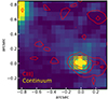 |
Fig. A.1. Map of the GN-z11 continuum around the CIII] emission line with the CIII] contours overlaid (red). Contours are 2, 4, 6, and 8 σ levels. The CIII] emission shows an extension to the East, while the continuum appears like a point source. |
Appendix B: Interlopers and other emission-line sources
We searched the region around GN-z11 for possible interlopers. There is a disc galaxy with bright Hα emission 1.1 arcsec north-east of GN-z11. We integrated the flux of this galaxy (dark red contours in Fig. B.1, left) and show the resulting spectrum (top-right panel). At the redshift of z = 2.028, there is no strong emission line that may contaminate the HeII emission (i.e. near λ = 1.90 μm). Besides, at the location of the HeII ‘clump’ (blue contours), the strength of any emission line due to the interloper would be even weaker than what is shown in the extracted spectrum. Conversely, if the putative HeII emission in the clump were due to some faint line associated with the galaxy at z = 2.028, then the spectrum extracted from the same aperture of the HeII clump would also show much stronger emission of Hα and the several other strong emission lines, which are not seen. We can therefore exclude that the line we identify as HeII is due to a misidentified faint line emission at z = 2.028.
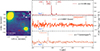 |
Fig. B.1. Map of the continuum in a region centred at the ‘haze’ highlighting a bright disc galaxy at z = 2, the haze itself, and a region south-west of GN-z11. The spectra of these three regions are shown in the right panels, highlighting the wavelength of our HeII detection, as well as other detected emission lines. The galaxy at z = 2 does not have any bright feature at wavelengths close to 1.902 μm. The haze presents a single emission line that we tentatively identify as [OIII]λ5007 at z = 3.66 – which would be consistent with the photometric redshift from Tacchella et al. (2023). Finally, we detected an emission line in the SW lobe of GN-z11. At the redshift of GN-z11, this line would correspond to a rest-frame wavelength of 0.1684 μm – which we do not trace to any notable emission line. |
The red contours show the extraction box around the ‘haze’ (cf. Tacchella et al. 2023). The corresponding spectrum shows an emission line at λ = 2.331 μm. We tentatively identify this line as either [OIII]λ5007 – typically the strongest emission line in low-mass galaxies. This would mean the ‘haze’ was a z = 3.665 interloper – consistent with the photometric redshift of Tacchella et al. (2023). If the line was Hα, we would expect to see [OIII]λ5007 at a bluer wavelength (low-mass galaxies typically have little dust), but no suitable emission was found. Either way, there is no strong emission line from this interloper near the wavelength of HeII.
We detected an emission line to the SW of GN-z11 (bottom panel of Fig. B.1). This source has no continuum and therefore no photometric redshift. We were thus unable to identify its redshift. Clearly, however, no contamination can arise from this region over to the HeII clump.
Finally, we note that the HeII emission of the clump has a very marginal feature (less than 2σ) to the red side of the line (at ∼1.907 μm). This does not match any other potential reasonably strong doublet or pair of lines that could be associated with a low-z interloper (e.g. Hα+[NII], [OII] doublet, [SII] doublet), not only in terms of wavelength separation but also because any reasonable pair of lines would imply the detection of a much stronger Hα emission at other wavelengths. If the weak, marginal feature is confirmed, this could be an additional weaker companion at ∼690 km/s from the main system, or it could be tracing an outflow component. However, we refrain from speculating further on this marginal feature, as its significance is very low and requires additional observations.
Appendix C: Spectrum extracted from large aperture excluding regions closer to GN-z11
The HeII emission in GN-z11 is so faint that it cannot contribute to the spectrum shown in the right panel of Fig.4 extracted from the large aperture drawn with a yellow box in Fig.1 (Tab.2); otherwise, many other much stronger lines from GN-z11 would be seen in the spectrum. In order to further exclude any contamination, we re-extracted the spectrum from the same aperture by excluding the region closer than 0.3″ (i.e. six times the radius of the PSF at this wavelength) from GN-z11. The resulting spectrum is shown in Fig.C.1, which is essentially unchanged with respect to Fig.4-right. If anything, the HeII detection is slightly more significant in this spectrum. Therefore, it is confirmed that the HeII flux from GN-z11 does not contribute to the flux observed in that aperture.
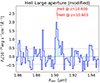 |
Fig. C.1. Spectrum extracted from the same extracted aperture at the spectrum in the right panel of Fig.4, that is, the aperture marked in yellow in Fig.1 (Tab.2), but where the regions closer than 0.3″ to GN-z11 were excluded. The spectrum is essentially unchanged with respect to the spectrum extracted from the entire aperture. |
Appendix D: Constraints on the HeII equivalent width
An important parameter in this work is the determination of the EW of HeII. In this Appendix, we provide some additional information on the methods to measure the EW.
As in most past spectroscopic studies at high redshift, inferring the EW directly from the spectra is extremely difficult, as the continuum is typically not detected in the spectrum. Therefore, most studies have resorted to inferring the continuum flux from photometry and combining it with the line flux inferred from the spectrum (e.g. Stark et al. 2017; De Barros et al. 2017; Mainali et al. 2018; Jung et al. 2020; Kusakabe et al. 2020). The availability of low-resolution spectroscopy with JWST has enabled detection of the continuum and measuring of the EW of lines directly in the spectra for a larger number of sources. However, with medium- and high-resolution spectroscopy, even with JWST, studies still have to rely on photometry to infer the EW of emission lines (e.g. Matthee et al. 2023), and for faint sources, photometry is still used to determine the EW of lines, even with JWST low-resolution spectroscopic modes (e.g. Boyett et al. 2022).
In this study we are in a similar regime. In the IFU spectra, the continuum is totally undetected, and the source is so faint that the continuum is marginally constrained in the low-resolution MSA spectrum. Therefore, our primary method to determine the EW was by using the photometric information from the NIRCam imaging (whose data processing is described in Tacchella et al. 2023). Photometry was extracted from the same apertures used for the extraction of the IFS spectra, as indicated in Fig.1. We did not attempt any PSF correction when extracting the photometry, as both apertures are much larger than the PSF at the wavelength of the redshifted HeII, and thus the PSF does not really affect the photometry. Additionally, we were not dealing with a strong spiky source, which could potentially cause significant PSF losses. Finally, the PSF at the same wavelength is similar for NIRCam and for NIRSpec, so any residual second-order losses from the aperture should be the same with the two instruments. The photometry uncertainty was inferred as in Tacchella et al. (2023); specifically, we added the uncertainties from the error map in quadrature, which gives the quoted error. We compared this to the variance of fluxes measured in empty (only sky, no sources) apertures of the same size in the mosaic and found that they are comparable (within 10%). The resulting continuum flux densities in the different apertures considered in this work are reported in Table 3. Given that the continuum is marginally detected even in photometry, we adopted an approach similar to Matthee et al. (2023) for determining the EW of high-z galaxies with JWST spectroscopy. Matthee et al. (2023) used the multi-band photometry to fit a Spectral Energy Distribution (SED) and then derived the continuum beneath the emission lines from the best-fit SED. In our case, the weak detections did not allow us to fit a proper SED. Moreover, using SED templates would imply making a priori assumptions on the nature of the continuum. We therefore adopted a simplified approach by inferring the continuum beneath the HeII with a linear interpolation of the photometry in the filters F150W, F200W, and F277W. We also provided a solid lower limit on the EW by using the tentative continuum detection, as inferred above from photometry, and adding a 2σ uncertainty, which gives the lower limit given in the main text of 20Å.
Finally, we reported the 3σ lower limit inferred from the non-detection of the continuum directly in the medium-resolution IFS spectrum. We also attempted to estimate the EW directly from the prism spectrum, given that in this case the continuum is marginally detected in the spectrum (and it has been fitted with linear function, masking the HeII line itself). The resulting values and lower limits are given in Table.1
Appendix E: NIRSpec-IFS vs NIRCam photometry comparison
Given that some of our estimates of the EW were performed by measuring the continuum from the photometry, it is important to verify the relative flux calibration of the NIRSpec spectra with the NIRCam images. The cross calibration between the MSA spectrum and photometry was already checked by Bunker et al. (2023) to be better than 5% for the prism, so we do not discuss it any further in this work.
Regarding the medium-resolution IFS spectra, we extracted the spectrum of GN-z11 from the same aperture 0.6″ as used by Tacchella et al. (2023) in the NIRCam image. From the spectrum, we extracted photometry in the F200W filter, which is the closest to the HeII redshifted wavelength. The aperture correction was applied, but with such a large aperture and at this wavelength, the correction is negligible. The resulting flux density is 141±17 nJy, which is consistent with the NIRCam photometric measurement of 144±2.7 nJy. The small difference between the two fluxes in both filters is well below the uncertainties resulting from the noise and background subtraction. Similarly, in the F277W filter, the flux density inferred from the IFS spectrum is 106±13 nJy, compared to 121.7±4.2 nJy in the NIRCam image.
All Tables
All Figures
|
Fig. 1. F277W NIRCam image of the central ∼1.7″ around GN-z11 illustrating the location of the MSA shutters during the first NIRSpec-MOS observations in February 2023 (tilted boxes; boxes of the same colour are associated with the same configuration), the extraction region of the HeII clump (red square), and the HeII extended emission (yellow box). The white circle indicates the absolute uncertainty of the MSA target acquisition (hence the shutters’ footprints are uncertain by this amount). North is up, and east is to the left. The orange vertical dashed line marks the boundary beyond which fewer dithers from the NIRSpec-IFU observations are available because of the guiding problem reported in Sect. 2. We note that the full IFU FoV is larger than shown here (> 3″ × 3″ taking into account the dithers). |
| In the text | |
|
Fig. 2. Prism spectrum of the region to the north-east of GN-z11, from the February 2023 MSA observation. Top panel: signal-to-noise 2D prism spectrum of GN-z11. The spectrum has been obtained by using only the exposures in which GN-z11 is in the upper and lower shutters (hence discarding the exposure with GN-z11 in the central shutter) as to avoid self-subtraction of the extended signal. Bottom panel: one-dimensional spectrum extracted from the region delimited by the two dashed horizontal lines, at about 0.45″ from GN-z11 in the NE direction, illustrating the tentative detection (3.7σ integrated) of a feature at 1.903 μm. The red vertical line indicates the location of HeIIλ1640 expected at the redshift of GN-z11, z = 10.603 (which is indistinguishable from the redshift of 10.600 inferred for the grating spectrum). |
| In the text | |
|
Fig. 3. Emission lines maps. Top panels: maps of the HeIIλ1640, Lyα, and CIII]λ1909 lines (see text for details). The red star marks the position of the continuum of GN-z11. Contours are at 2, 3, and 4σ for the HeII and Lyα maps and at 2, 4, 6, and 8σ for the CIII] map (the rms is estimated from the statistics in the IFU FoV, outside this region). We note that most of these spaxels are independent; hence the significance of the integrated emission of each feature is significantly higher. The two white boxes indicate the extraction apertures of the two spectra shown in Fig. 4 and marked in red and yellow in Fig. 1. The vertical dashed segment indicates the region beyond which there are fewer exposures because of the guiding problem discussed in Sect. 2. Bottom panels: overlay of the contours from the emission line maps onto the F277W NIRCam map from Tacchella et al. (2023). |
| In the text | |
|
Fig. 4. Spectra extracted from the apertures indicated in Fig. 1 and zoomed near the expected wavelength of HeII at the redshift of GN-z11. Specifically, the left panel shows the spectrum extracted from the aperture centred on the ‘HeII clump’ (red box in Fig. 1 and smaller white box in Fig. 3). The right panel shows the spectrum extracted from the larger aperture encompassing the extended HeII emission in the NE quadrant of GN-z11 (yellow box in Fig. 1 and larger white box in Fig. 3). The red vertical bars indicate the expected wavelength of HeII at the redshift of GN-z11, z = 10.603, and the wavelength of the centroid of the line in the clump, which, if identified as HeII, gives a redshift z = 10.600. The dotted lines indicate the noise per spectral pixel in each spectrum inferred from the rms directly measured in the spectrum around the HeII line. |
| In the text | |
|
Fig. 5. Observed HeIIλ1640 luminosity of the ‘HeII clump’ and its projected distance from GN-z11 compared to the expected HeII luminosity as a function of distance from GN-z11, in case of AGN photoionisation. In this calculation, we used the upper limit for the size of the HeII clump and assumed a broad range of AGN ionising shapes powering the photoionisation. Further conservative assumptions are that the ‘HeII clump’ is not made of unresolved clumps and that the projected distance is the actual separation. Clearly, the HeII luminosity observed in the ‘HeII clump’ is inconsistent with being photoionised by the AGN in GN-z11. |
| In the text | |
|
Fig. 6. Diagnostic diagrams showing the EW of HeIIλ1640 versus various line ratios: HeII/Hγ, CIVλ1550/HeII, CIII]1909/HeII, and OIII]λ1665/HeII. The observational constraints on the HeII clump in the halo of GN-z11 are shown with golden symbols, while the observational constraints for the HeII emission obtained from the large aperture extraction are shown with green symbols. Circles are for EWs for which the continuum has been inferred from photometry, while squares show the EWs for which the continuum constraints have been inferred directly from the spectra. Purple stars show PopII models with different (absolute) metallicities (colour-coded with different purple shadings) and where the gas and stars are assumed to have the same metallicity. Blue circles are models of PopIII stars in a pristine gas; light blue squares are models of PopIII stars in a mildly enriched gas, specifically Zgas = 10−5; light blue triangles are models of PopIII stars in a more enriched gas, specifically Zgas = 10−4. The PopIII markers have different sizes depending on the stellar mass range assumed for the IMF, as indicated in the legend. Orange pentagons show the predictions for accreting DCBHs embedded in gas with different (absolute) metallicities. |
| In the text | |
|
Fig. A.1. Map of the GN-z11 continuum around the CIII] emission line with the CIII] contours overlaid (red). Contours are 2, 4, 6, and 8 σ levels. The CIII] emission shows an extension to the East, while the continuum appears like a point source. |
| In the text | |
|
Fig. B.1. Map of the continuum in a region centred at the ‘haze’ highlighting a bright disc galaxy at z = 2, the haze itself, and a region south-west of GN-z11. The spectra of these three regions are shown in the right panels, highlighting the wavelength of our HeII detection, as well as other detected emission lines. The galaxy at z = 2 does not have any bright feature at wavelengths close to 1.902 μm. The haze presents a single emission line that we tentatively identify as [OIII]λ5007 at z = 3.66 – which would be consistent with the photometric redshift from Tacchella et al. (2023). Finally, we detected an emission line in the SW lobe of GN-z11. At the redshift of GN-z11, this line would correspond to a rest-frame wavelength of 0.1684 μm – which we do not trace to any notable emission line. |
| In the text | |
|
Fig. C.1. Spectrum extracted from the same extracted aperture at the spectrum in the right panel of Fig.4, that is, the aperture marked in yellow in Fig.1 (Tab.2), but where the regions closer than 0.3″ to GN-z11 were excluded. The spectrum is essentially unchanged with respect to the spectrum extracted from the entire aperture. |
| In the text | |
Current usage metrics show cumulative count of Article Views (full-text article views including HTML views, PDF and ePub downloads, according to the available data) and Abstracts Views on Vision4Press platform.
Data correspond to usage on the plateform after 2015. The current usage metrics is available 48-96 hours after online publication and is updated daily on week days.
Initial download of the metrics may take a while.