| Issue |
A&A
Volume 687, July 2024
|
|
|---|---|---|
| Article Number | A116 | |
| Number of page(s) | 34 | |
| Section | Stellar structure and evolution | |
| DOI | https://doi.org/10.1051/0004-6361/202244066 | |
| Published online | 02 July 2024 | |
Absolute dimensions of solar-type eclipsing binaries
NY Hya: A test for magnetic stellar evolution models⋆
1
University of Southern Denmark, Department of Physics, Chemistry and Pharmacy, SDU-Galaxy, Campusvej 55, 5230 Odense M, Denmark
e-mail: tchinse@gmail.com
2
Ankara University, Faculty of Science, Department of Astronomy and Space Sciences, Tandoğan, 06100 Ankara, Türkiye
3
Ankara University, Astronomy and Space Sciences Research and Application Center (Kreiken Observatory), İncek Blvd., 06837 Ahlatlıbel, Ankara, Türkiye
4
Astrophysics Group, Keele University, Staffordshire ST5 5BG, UK
5
Department of Physics & Astronomy, University of North Georgia, Dahlonega, GA 30597, USA
6
Instituto de Investigación en Astronomia y Ciencias Planetarias, Universidad de Atacama, Avenida Copayapu 485, Copiapó, Atacama, Chile
7
NASA Goddard Space Flight Center, 8800 Greenbelt Road, Greenbelt, MD 20771, USA
8
SETI Institute, 189 Bernardo Ave, Suite 200, Mountain View, CA 94043, USA
9
Astrobiology Center, NINS, 2-21-1 Osawa, Mitaka, Tokyo 181-8588, Japan
10
National Astronomical Observatory of Japan, NINS, 2-21-1 Osawa, Mitaka, Tokyo 181-8588, Japan
11
Astronomical Science Program, Graduate University for Advanced Studies, SOKENDAI, 2-21-1, Osawa, Mitaka, Tokyo 181-8588, Japan
12
Ankara University, Graduate School of Natural and Applied Sciences, Department of Astronomy and Space Sciences, Tandoğan, 06100 Ankara, Türkiye
13
Astronomical Institute of the Czech Academy of Sciences, 251 65 Ondřejov, Czech Republic
14
Institut de Ciències de l’Espai (ICE, CSIC), Campus UAB, c/ Can Magrans s/n, 08193 Bellaterra, (Barcelona), Spain
15
Institut d’Estudis Espacials de Catalunya (IEEC), Edifici RDIT, Campus UPC, 08860 Castelldefels, (Barcelona), Spain
16
Niels Bohr Institute, University of Copenhagen, Jagtvej 155, 2200 Copenhagen, Denmark
17
Chungnam National University, Department of Astronomy, Space Science and Geology, Daejeon, Republic of Korea
18
Landessternwarte, Zentrum für Astronomie der Universität Heidelberg, 69117 Heidelberg, Germany
19
Center for Space and Habitability, University of Bern, Gesellschaftsstrasse 6, 3012 Bern, Switzerland
20
McGill Space Institute, McGill University, 3550 University Street, Montreal, QC H3A 2A7, Canada
21
Department of Astronomy, Arthur C. Clarke Institute for Modern Technologies, 0272 Moratuwa, Sri Lanka
22
Centre for ExoLife Sciences, Niels Bohr Institute, University of Copenhagen, Øster Voldgade 5, 1350 Copenhagen, Denmark
23
University of St Andrews, Centre for Exoplanet Science, SUPA School of Physics & Astronomy, North Haugh, St Andrews KY16 9SS, UK
24
Centre for Electronic Imaging, School of Physical Sciences, The Open University, Milton Keynes MK7 6AA, UK
25
Instituto de Astrofísica e Ciências do Espaço, Departamento de Física, Universidade de Coimbra, 3040-004 Coimbra, Portugal
26
Centro de Astronomía, Universidad de Antofagasta, Avenida Angamos 601, Antofagasta 1270300, Chile
27
Chungbuk National University Observatory, Chungbuk National University, 28644 Cheongju, South Korea
28
Department of Astronomy and Atmospheric Sciences, Kyungpook National University, 41566 Daegu, South Korea
29
Department of Physics, College of Science, Princess Nourah bint Abdulrahman University PO Box 84428 Riyadh 11671, Saudi Arabia
30
Department of Physics, School of Science, Aristotle University of Thessaloniki, 541 24 Thessaloniki, Greece
31
S.M. Nikolskii Mathematical Institute of the Peoples’ Friendship University of Russia (RUDN University), Moscow 117198, Russia
Received:
20
May
2022
Accepted:
21
March
2024
Context. The binary star NY Hya is a bright, detached, double-lined eclipsing system with an orbital period of just under five days with two components each nearly identical to the Sun and located in the solar neighbourhood.
Aims. The objective of this study is to test and confront various stellar evolution models for solar-type stars based on accurate measurements of stellar mass and radius.
Methods. We present new ground-based spectroscopic and photometric as well as high-precision space-based photometric and astrometric data from which we derive orbital as well as physical properties of the components via the method of least-squares minimisation based on a standard binary model valid for two detached components. Classic statistical techniques were invoked to test the significance of model parameters. Additional empirical evidence was compiled from the public domain; the derived system properties were compared with archival broad-band photometry data enabling a measurement of the system’s spectral energy distribution that allowed an independent estimate of stellar properties. We also utilised semi-empirical calibration methods to derive atmospheric properties from Strömgren photometry and related colour indices.
Results. We measured (percentages are fractional uncertainties) masses, radii, and effective temperatures of the two stars in NY Hya and found them to be MA = 1.1605 ± 0.0090 M⊙ (0.78%), RA = 1.407 ± 0.015 R⊙ (1.1%), Teff, A = 5595 ± 61 K (1.09%), MB = 1.1678 ± 0.0096 M⊙ (0.82%), RB = 1.406 ± 0.017 R⊙ (1.2%), and Teff, B = 5607 ± 61 K (1.09%). The atmospheric properties from Strömgren photometry agree well with spectroscopic results. No evidence was found for nearby companions from high-resolution imaging. A detailed analysis of space-based data revealed a small but significant eccentricity (e cos ω) of the orbit. The spectroscopic and frequency analysis on photometric time series data reveal evidence of clear photospheric activity on both components likely in the form of star spots caused by magnetic activity.
Conclusions. We confronted the observed physical properties with classic and magnetic stellar evolution models. Classic models yielded both young pre-main-sequence and old main-sequence turn-off solutions with the two components at super-solar metallicities, in disagreement with observations. Based on chromospheric activity and X-ray observations, we invoke magnetic models. While magnetic fields are likely to play an important role, we still encounter problems in explaining adequately the observed properties. To reconcile the observed tensions we also considered the effects of star spots known to mimic magnetic inhibition of convection. Encouraging results were obtained, although unrealistically large spots were required on each component. Overall we conclude that NY Hya proves to be complex in nature, and requires additional follow-up work aiming at a more accurate determination of stellar effective temperature and metallicity.
Key words: binaries: eclipsing / binaries: spectroscopic / stars: fundamental parameters / stars: individual: HD80747 / / stars: solar-type
© The Authors 2024
 Open Access article, published by EDP Sciences, under the terms of the Creative Commons Attribution License (https://creativecommons.org/licenses/by/4.0), which permits unrestricted use, distribution, and reproduction in any medium, provided the original work is properly cited.
This article is published in open access under the Subscribe to Open model. Subscribe to A&A to support open access publication.
1. Introduction
Stellar components in a detached eclipsing binary (dEB) system provide a direct empirical measure of their physical properties with a minimum number of assumptions. From photometric and double-lined spectroscopic data, the masses and radii can be determined providing an empirical test of stellar evolution models. The most strict model tests are for those systems where elemental abundances are determined spectroscopically, reducing the number of free parameters to the fractional helium content, age and model-internal parameters (Andersen 1991). Secure astrophysical information about system properties is further substantiated with recent space-based astrometric distance measurements (Stassun & Torres 2021) allowing a reliable measurement of system properties without limiting assumptions; in pre-Gaia times nearby eclipsing binaries were used as reliable distance estimators. Detached systems are therefore of fundamental astrophysical importance and constitute the primary source of knowledge of properties of individual stars to form the test bed when confronting stellar evolution theory. From high-quality photometry and spectroscopy, the stellar masses and radii can be determined to better than 1% precision from in-depth analyses of eclipse light curves and double-lined radial velocity (RV) curves with good phase coverage (Torres et al. 1997; Southworth et al. 2005b). The reliable measurement of accurate stellar properties is further increased for systems located in the solar neighbourhood where interstellar reddening effects are small.
As pointed out by Southworth & Clausen (2007), stellar evolution models are generally good at predicting the physical properties of stars (see Maxted et al. 2015) for two reasons. First, the effects of improved input physics often result in only small adjustments in the evolutionary phases for the two components. Second, some model parameters that are not known independently (or are harder to infer empirically) can be freely adjusted in order to match the observed properties. The additional parameters are helium abundance and age, as well as input-physics parameters describing convective core overshooting, mixing length, mass loss, and various treatments of opacity (Cassisi 2005). While some parameters, such as stellar abundances (from a careful abundance analysis) and age (in the case of cluster membership or by other means such as chromospheric activity, gyrochronology, or depletion of certain age-dependent species) can be inferred empirically, thus providing additional constraints on the investigated model, this is not always the case. Therefore, the second aspect is worrying, since it is hard to identify and test physical mechanisms governing stellar evolution given the extra degrees of freedom in adjusting and tweaking one or more parameters.
For lower-mass detached eclipsing binary stars, discrepancies between the observed properties and model predictions have been noted in the literature for stars of spectral types G to M (Popper 1997; Torres & Ribas 2002; Ribas 2003; Clausen et al. 2009; Southworth 2022). This implies that the principles of single-star stellar evolution do not fully apply to stars in a detached eclipsing system; often the predicted effective temperature (Teff) are too high for the observed masses or, for a fixed age, the predicted radii are too small, whilst masses and radii are measured with fractional uncertainties to 1% or better. Further, in the case when no independent age constraint is available, the models fail in placing the two components on the same isochrone in the stellar radius-mass (R − M) plane.
In an attempt to reconcile certain stellar evolution models with observations, the usual approach is the computation of dedicated model grids for which the mixing length parameter (l/Hp) is adjusted for each component and compared to observations. Often this results in a success in matching the observed properties (Vos et al. 2012), but highlights the aforementioned worries: input physics parameters are adjusted until a good match was found, which concludes the analysis. However, while the observations, within observational errors, were adequately described, the explanation was only described at a phenomenological level without properly addressing an adequate physical mechanism.
The short-coming of solar-type evolution models to properly describe solar-type components is to be found in the fast rotation of short-period detached binaries. For short-period eclipsing binaries tidal interactions have resulted in an increased stellar rotation spin-up to a pseudo-synchronous state (1:1 spin-orbit resonance; Hut 1981; Li 2018). Rotation velocities (v sin i) for single solar-type stars are of the order of 1 km s−1 or lower. The rotation velocities of similar stars in an eclipsing system are found to be 10 km s−1 or higher. The fast rotation is thought to have a significant effect on the convective energy transport (Chabrier et al. 2007). Qualitatively, in mixing-length theory, convection is described by the mixing-length parameter and is capable of phenomenologically addressing the often neglected and complicated effects of magnetic fields; for fast rotators a strong magnetic field is generated, which triggers the Lorentz force to act on the outer material region of the convection zone, thereby decreasing its convective height. Thus, by adjusting l/Hp one has the option to indirectly describe the effect of a magnetic field on the convective region. However, a more realistic treatment of this problem is to directly include the effect of a magnetic field in stellar evolution models. Magnetic fields are often ignored and, as shown recently, are capable of providing a viable physical mechanism to explain observed discrepancies (Feiden & Chaboyer 2012).
In this work we present and analyse for the first time high-quality light curves (TESS) and high-resolution spectroscopic (FEROS) observations of NY Hya. The bright (V = 8.58 mag) stellar object HD 80747 (NY Hya, BD-06 2891, HIP 45887) was discovered by the HIPPARCOS mission (ESA 1997) to be an eclipsing binary and subsequently named NY Hya by Kazarovets et al. (1999). The HIPPARCOS parallax places NY Hya at a distance of 81.8 ± 8.6 pc. In the Henry Draper Catalogue, Cannon & Pickering (1993) classified NY Hya as a G5 star without any remarks to its binary nature.
Dedicated photometric follow-up observations in the Strömgren system were reported in Clausen et al. (2001), establishing the first accurate ephemeris and announcing a significant update on the orbital period (4.77 days) compared to the period determined from the HIPPARCOS data. The ephemeris was further updated by Kreiner (2004) and Pojmanski (1997) with the latter providing instrumental V-band data as part of their All Sky Automated Survey (ASAS). The Strömgren-Crawford uvbyβ photometry catalogue by Paunzen (2015) provides entries for the Strömgren indices of NY Hya. No β measurement was given. The data are based on a single measurement, and are therefore questionable. No reliable uncertainties are provided. Therefore, we suggest that the Strömgren data should be taken from Clausen et al. (2001; see Table 1). For a (b − y) = 0.444 mag (without reddening correction) we determine the spectral type of NY Hya to be G6V, or G5V (Olsen 1984, Table V) with a correction for extinction (see Sect. 6.3). The Michigan catalogue of HD stars (Houk & Swift 1999) lists a spectral type of G5V.
Photometric data for NY Hya and the comparison stars HD 82074, HD 80446, and HD 80633.
The eclipsing system NY Hya belongs to the class of fast rotators and classic stellar models (as investigated here) are not able to describe the observed physical properties of this system. A closer look at the X-ray emission of NY Hya indicates a high chromospheric activity level indicating the presence of a magnetic field. This finding is further supported by a significant intrinsic photometric variability most readily seen during out-of-eclipse phases mostly due to the changing appearance of star spots. However, significant progress has been made in recent years in the development of stellar evolution models considering the effect of a magnetic field. We therefore apply state-of-the-art evolution models (Feiden & Chaboyer 2012) to the observed physical properties, providing a more rigorous benchmark to test formerly neglected input physics.
The paper is structured as follows. In Sect. 2 we present new observations including TESS photometry and high-resolution FEROS spectra. In Sect. 3 we analyze the spectra to derive empirical spectroscopic light ratios and measure radial velocities. In Sect. 4 we present an updated and improved ephemeris thanks to the TESS data. A complete analysis of the light and radial velocity curves is presented in Sect. 5. Then we determine the physical parameters of the system and its components through a rigorous spectroscopic analysis of the spectra we disentangled in Sect. 6. In Sect. 7 we compile intermediate- and broad-band photometry from the literature (which we corrected for the interstellar extinction in Sect. 6.3) and present the results obtained from an analysis of the spectral energy distribution (SED) considering NY Hya as a single star. This provides a mean estimate for the Teff providing an independent consistency check on the spectroscopy. In Sect. 8 we carry out a period analysis based on the out-of-eclipse variability. We were able to independently determine the orbital period from the presence of surface spots; this allowed us to conclude synchronous rotation via tidal locking of the two components. In Sect. 9 we utilize Gaia astrometry to infer kinematical properties of NY Hya in an attempt to determine stellar age via cluster-membership identification. In Sect. 10 we compare the observed properties of the two components with stellar evolution models. We invoke both classic and non-standard magnetic models. We substantiate the importance of magnetic fields by providing a semi-empirical estimate of magnetic field strength from observations of the total X-ray luminosity. Finally, we present our conclusions in Sect. 11.
2. Observations
We present Strömgren photometry from the literature, high-precision and high-cadence space-based observations from the TESS telescope, high-resolution lucky-imaging, and high-quality spectra from the FEROS spectrograph. Additional archival photometric data are presented in Sect. 7 as part of a SED analysis.
2.1. Strömgren photometry
Photometric data were obtained by Clausen et al. (2001) using the (now decommissioned) 0.5m Strömgren Automatic Telescope (SAT) at the ESO/La Silla observatory (Florentin-Nielsen et al. 1987) during two observing seasons: Season 1, spanning from November 23, 1997 (JD 2 450 775.8), to April 28, 1998 (JD 2 450 931.6), and Season 2, spanning from October 12, 1998 (JD 2 451 098.9), to March 16, 1999 (JD 2 451 253.7). All comparison stars, relevant photometric data for which are provided in Table 1, were found to be constant with respect to the check star, HD 80633. In particular, Lockwood et al. (1997) found HD 82074 to be stable in their long-term photometric variability program of solar-type stars.
The SAT data reduction follows an equivalent procedure as described in Clausen et al. (2001, 2008). Here we add a few more details. To form the final photometry for the comparison stars (C1, C2) a 2.5σ−clipping was applied to remove 44 outliers. A total of 19 measurements were discarded by this criterion when forming the C1-C2 magnitude level. Linear extinction coefficients were determined from the comparison stars for each night and apparent magnitudes corrected accordingly. The maximum and minimum root-mean-square errors between the comparison stars was 7.6 mmag and 4.6 mmag, respectively depending on Moon illumination, airmass and sky conditions. Photometric root-mean-square errors for NY Hya SAT observations were found to be 3.7 mmag (u band) and 2.2 mmag (vby bands).
The instrumental uvbyβ system at the SAT was found to be long-term stable (Clausen et al. 2001) from observing uvbyβ standard stars. This implies that no transformation to the standard uvbyβ system was needed to form differential (uvby) light curves in the instrument system having the additional advantage of avoiding additional photometric errors introduced via transformation relations. Atmospheric extinction and detector temperature variations were corrected for Clausen et al. (2001). However, based on numerous bright standard stars observed each night, standard Johnson V and standard Strömgren indices (b − y, m1, c1 and β) for NY Hya were determined at all orbital phases. See Table 1 for details. We note only minuscule colour differences between the two components during primary and secondary eclipses indicating near-equal Teffs.
Original time stamps (HJD) of all SAT observations refer to the midpoint of the integration time interval. We have transformed the HJD times in the UTC time standard to BJD times in the TDB time standard using the online time conversion1 provided by Eastman et al. (2010). This was necessary in order to have a consistent time standard as the SAT eclipse minimum timings were later combined with space-based photometry.
2.2. Space-based TESS observations
NY Hya was observed by the TESS (Transiting Exoplanet Survey Satellite) space telescope (Ricker et al. 2009, 2014, 2015). NY Hya was observed at a 2 min cadence in Sector 8 with Camera 1 and CCD 1. The photometric data were retrieved from MAST2 (Mikulski Archive for Space Telescopes) using LIGHTKURVE (Lightkurve Collaboration 2018; Dotson et al. 2019). Since NY Hya is a binary system the SAP (Simple Aperture Photometry) light curve was extracted. We discarded photometric measurements with the following data quality flags: ‘attitude tweak’, ‘safe mode’, ‘coarse point’, ‘Earth point’, ‘desat’, and ‘manual exclude’ (see TESS science data products description3). The SAP light curve is produced by TESS SPOC (Science Processing Operations Center; Jenkins et al. 2016) designed for producing optimal aperture photometry.
Figure 1 shows a pixel-mosaic image of the first cadence for NY Hya along with the target aperture mask. The data release notes4 for sector 8 describe that an instrument anomaly began at UTC 2019-02-17 05:48:35 which ceased all data and telemetry collection. Normal operations resumed at 2019-02-20 12:02:38. Data collection was paused for 1.19 days during perigee passage while downloading data. The ‘release notes’ for Sector 8 also describe how Camera 1 was affected by scattered light from the Earth and Moon. The background pixels were primarily affected at the end of the two orbits by Earth and towards the start of orbit 24 by the Moon.
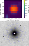 |
Fig. 1. Photometric images of NY Hya from two different instruments. Top panel: camera 1 and CCD 1 target pixel file image of the first TESS cadence for NY Hya. The TESS target aperture mask used to generate the SAP light curve is highlighted in red. Bottom panel: SAP aperture superimposed on a Pan-STARRS image. North is up and east is left. Each box is 21 × 21 arcsec in size. Three faint companions are positioned at around 22 arcsec from NY Hya. |
Because the available data affected by the scattered light do not contain an eclipse we masked the data between BJD 2 458 530.0 and 2 458 536.3, resulting in a 6.3 day data gap. We show the resulting SAP light curve in Fig. 2.
 |
Fig. 2. Extracted TESS SAP light curve of NY Hya from Sector 8 with a sampling of 2 min. The first eclipse is a primary eclipse. Five primary and three secondary eclipses were observed. Some out-of-eclipse variation is clearly detected. The increase in flux at BJD 2 458 536 changes depending on the parameters used in the LIGHTKURVE detrending process. We therefore believe that this is systematic noise. |
Due to TESS having a large pixel scale (21 arcsec pixel−1), it is important to check for faint nearby stars which may contaminate the point spread function (PSF) of the target star. To do this, we follow the procedure given by Swayne et al. (2020). We overlaid the TESS target aperture mask over an image of NY Hya from the Pan-STARRS image server (Flewelling 2016), which indicated that three faint objects (lower three pixels) are within the TESS aperture mask used by SPOC. We cross-referenced these objects with the TESS input catalogue (Stassun et al. 2018, 2019). The brightest two were found to have a TESS magnitude of 16 and 19 (NY Hya has a TESS magnitude of 8) which translates to 1600 and 25 000 times fainter than NY Hya providing a total contribution of flux of approximately 0.01% and hence these sources are negligible. The faintest of the three is not in the TESS input catalogue, indicating that it is fainter than TESS magnitude 19.
The Gaia Data Release 2 (DR2; Gaia Collaboration 2018) indicates the presence of a nearby star (Gaia 5746104876937814912) that is 6 arcsec from NY Hya and has since been confirmed to have the same parallax as NY Hya, from the Gaia Early Data Release 3 (EDR3; Gaia Collaboration 2021). When compared with the Pan-STARRS image (Fig. 1) the companion lies within the saturated pixels of NY Hya and therefore, lies within the TESS target aperture. Consequently, we crossed-referenced the companion star with the TESS input catalogue and found the companion (TIC 876368206) to have a TESS magnitude of 16.5, indicating a negligible (≈0.01%) contribution to the measured flux.
2.3. EMCCD lucky-imaging observations
We further obtained high-resolution imaging data with the purpose to detect nearby companions that could be the source of observed photometric signals or the dilution of such signals. NY Hya was observed on the beginning night of May 21, 2019 and May 23, 2021 with the two-colour instrument (TCI; v and z bands) attached to the Danish 1.54 m telescope at the ESO/La Silla Observatory, Chile. For optimal detection, all (May 21, 2019) images were obtained at airmass 1.10 with a seeing of < 1 arcsec. The observations were conducted as part of the 2019/2021 MiNDSTEp5 campaign. Each TCI consists of a 512 × 512 pixel electron-multiplying (Andor, iXon+897) CCD capable of imaging simultaneously in two colours. The field of view is about 45 × 45 arcsec yielding a pixel scale of approximately 0.09 arcsec pixel−1. A detailed description of the instrument and the lucky-imaging reduction pipeline is given in Skottfelt et al. (2015).
The observations and data reduction were carried out using the methods outlined as follows, which resemble the methods described by Evans et al. (2016). The exposure times of the targets in the high-resolution imaging observations were selected to detect (at 5-σ) a star up to 5 mag fainter than the target in V. Fainter stars can be safely ignored as their contamination to the eclipse depth would be < 0.1 mmag, which is less than the RMS noise (0.382 mmag) of the TESS data presented in this work. NY Hya was observed for 120 s at a frame rate of 10 Hz, allowing for near-diffraction limited images to be constructed by combining only frames with the least atmospheric distortion. The raw data were reduced by a custom pipeline that performs bias and flat frame corrections, removal of cosmic rays, determination of the quality of each frame and frame re-centring. The end product consists of ten sets of stacked frames ordered by quality.
We computed 5σ contrast curves from image statistics for each camera from selecting the first 20% best images (i.e. stacked the first 240 frames) and summed flux contributions from each pixel in concentric rings centred on the star’s location as determined by a two dimensional Gaussian fit to the point spread function and extending radially away from the star. We used a cubic spline to smooth the contrast in delta magnitudes as a function of separation, assuming a minimum of 5σ for the detection of a point source. The resulting contrast curves are shown in Fig. 3. We detect a small brightness increase of Δmag = 7.5 at a separation of about 14 arcsec in the v-band camera. At this point, we are not sure whether this is instrumental or caused by the faint nearby companions as shown in Fig. 1.
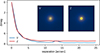 |
Fig. 3. 5σ detection contrast-curves (Δmag) from the TCI images using the top 20% stacked frames. Inset images are 10 × 10 arcsec. The full width at half maximum (seeing) was measured to be 0.97 arcsec in v and 0.85 arcsec in z. |
The nearby companion at 6 arcsec that was detected in the Gaia DR2 and EDR3 was not detected in the presented high-resolution imaging data, which is expected considering the companion is approximately 8.5 magnitudes fainter than NY Hya in the TESS bandpass which has a similar central wavelength to the z-band camera.
2.4. Spectroscopic observations
Ribas (1999, his Table 2.4) presented and analysed 22 unpublished RV (CORAVEL scanner, decommissioned) measurements (σRV = 0.5 km s−1 per measurement). Ribas (1999) found NY Hya to be a double-lined spectroscopic binary and derived preliminary spectroscopic elements. He found two components (NY Hya A and B), near-identical in minimum mass, orbiting each other in a circular orbit with a systemic RV of around 40 km s−1. The spectroscopic orbital period agrees with the Clausen et al. (2001) value (0.015σ). Unfortunately, a complete simultaneous photometric and spectroscopic analysis of NY Hya was never presented in the literature. Furthermore, a check in the Detached Eclipsing Binary Catalogue (DEBCat6; Southworth et al. 2015) revealed no information on NY Hya.
A total of 35 high-resolution spectra were obtained of NY Hya using the ESO 1.52 m telescope and the Fibre-fed Extended Range Optical Spectrograph (FEROS;7, Kaufer et al. 1999) at the ESO/La Silla observatory, Chile. The resolving power of FEROS is λ/Δλ = 48 000 (constant velocity offset of 2.2 km s−1/pix) covering an effective wavelength range of 3600–9200 Å starting from the Balmer discontinuity and spanning 39 échelle orders. The object-sky (OS) observing mode was used for the two fibre apertures for optimal background subtraction. The entrance aperture of each fibre is 2.6 arcsec. The minimum and maximum standard error for the wavelength calibration (all nights) was 0.007 Å and 0.019 Å, respectively.
Observations were carried out as part of the FEROS commissioning and guaranteed time period (commissioning II and 62.H-0319/GT I) between November 23, 1998 and January 21, 1999. All spectra obtained during the two commissioning periods are public and were retrieved from the FEROS spectroscopic database hosted at the Landessternwarte Heidelberg8. During observations, the spectrograph was located in a temperature-controlled vacuum chamber. Typically, calibration frames were obtained at the beginning, middle and end of the night resulting in an average to account for thermal drift and environmental changes. Wavelength scales were established on a nightly basis from Thorium-Argon (Th-Ar) exposures. Pre-normalisation fluxes are relative fluxes (object/flat). In Table A.1 we list details of the nightly observed FEROS spectra.
Raw spectral data reduction was performed with the ESO MIDAS9 package. The spectra are available as standard reduced (i.e. standard, not optimal), order-extracted, flat-fielded, bias-subtracted (from between orders), wavelength calibrated (barycentric rather than heliocentric correction to the wavelength scale is applied at the re-binning stage of the échelle orders) one-dimensional flux tabulated spectra. The instrumental blaze function was removed to first order using the flat exposure. Removal of scattered light was applied. Exposure times10 were either 420 s, 600 s or 900 s with the vast majority (32) of spectra taken with 600s resulting in a signal-to-noise (S/N) ratio in the range 174–261. We had to discard two spectra entirely (#2266 at the orbital phase 0.31 and #2912 at 0.27) due to low quality and wavelength calibration problems in the data. Since we have several high-quality spectra in this orbital phase range (four others between phases 0.24 and 0.35) the coverage of orbital phase is still good.
2.5. Identities of the two stars
The standard definitions are that the primary eclipse is deeper than the secondary eclipse, and that the primary star is eclipsed at primary eclipse. We follow these conventions here, but with caveats. The two stars are almost identical, and starspots affect the light curve shape, so choosing which is the primary is not trivial. We inspected the three TESS sectors and found that one type of minimum is clearly deeper than the other in two cases; we label this the primary eclipse. In the third TESS sector starspot activity causes the primary and secondary eclipses to be of almost identical depth. The greater scatter in the uvby light curves means the eclipse depths are not significantly different in those data.
The orbital ephemeris given below (Eq. (1) in Sect. 4) defines our identification of the stars. Orbital phase zero in this ephemeris corresponds to the primary eclipse and is where the primary star is eclipsed by the secondary star. We refer to the primary as star A in the following analysis, and its companion as star B. These identifications are consistent with the ephemeris given by Clausen et al. (2001). We ultimately find that the masses, radii and temperatures of the two stars are so similar as to be identical to within their uncertainties.
3. Radial velocity and light ratio determination
3.1. Continuum normalisation
All FEROS spectra were normalised to the continuum level iteratively and via interactive comparisons with a synthetic spectrum computed using the SYNTH3 code (Kochukhov 2007) which is based on ATLAS/SYNTHE program suite of Kurucz (1993), the SYNTH and SYNTHMAG codes of Piskunov (1992) and the SME program written by Valenti & Piskunov (1996). We made use of the Vienna Atomic Line Database (VALD; Piskunov et al. 1995) for line identification and initial estimates for the fundamental atmospheric parameters for both components (Teff = 5700 K, log g = 4.15 (cgs), [Fe/H] = 0.0 dex). The Teff, log g, and [Fe/H] were obtained from Strömgren photometry and a preliminary SED analysis (see Sect. 7) to obtain composite spectra for different orbital phases matching that of the observations for continuum normalisation. We then compared these spectra with the FEROS spectra visually by using the BINMAG6 code (Kochukhov 2018) and continuum-normalised our observational spectra.
We examined four different wavelength regions centred on the Strömgren (vby) and TESS passbands to normalise the observed spectra. Wavelength ranges of these segments correspond to the Full Width at Half Maximum (FWHM) of the passband response curves (Rodrigo et al. 2012; Rodrigo & Solano 2013). We made use of interactive IDL widgets XREGISTER_1D.PRO and LINE_NORM.PRO in the FUSE11 package, respectively, for cosmic-ray removal and continuum normalisation.
We measured the signal-to-noise (S/N) with relevant tools in the GUIAPPS package of the IRAF package12 from different segments of the continuum and averaged them. We double-checked our measurements by also employing the ‘SNR Estimator’ in the current version of the ISPEC13 software package (Blanco-Cuaresma et al. 2014; Blanco-Cuaresma 2019).
3.2. Radial velocities
RVs were measured using i) one-dimensional cross-correlation functions (CCFs, Tonry & Davis 1979), ii) Rucinski’s broadening functions (Rucinski 1999), and iii) the two-dimensional cross-correlation technique (hereafter TODCOR; Mazeh & Zucker 1994) in 160−250 Å wide spectral windows. Similar results were obtained from all three methods lending confidence in the accuracy of our RV measurements.
In this work, we chose to present and adopt measurements obtained from TODCOR since this technique provides the additional option to measure a light ratio (luminosity or flux ratio) for selected spectral windows. Estimates of the spectral light ratios will be beneficial in the analysis of light curves (see Sect. 5.2) as discussed later. The TODCOR technique aims to correlate an observed binary spectrum against a combination of two template spectra with all possible RV shifts to determine the unknown wavelength displacements in the spectra of each individual component at any orbital phase. Therefore, the correlation is a two-dimensional function of the velocity shifts of the two templates. The position of the correlation maxima corresponds to the RVs of individual components. TODCOR has the advantage over the traditional one-dimensional cross correlation in the determination of the correlation maxima even when blends of the correlation peaks are inevitable and for the case when one companion is significantly fainter than the other.
We applied the TODCOR technique to wavelength regions in close agreement with the Strömgren and TESS filter14 transmission profiles (Rodrigo et al. 2012; Rodrigo & Solano 2013, 2020; v: 4030−4190 Å, b: 4570−4770 Å, y: 5360−5600 Å and 7850−8100 Å for the TESS filter). We made use of synthetic spectra as templates for each of the stars that were generated for spectral normalisation. We experimented with templates accounting for the rotational broadening as well, but in line with other CCF-based techniques relying on delta-functions, we ignored stellar rotation during the synthesis of our templates to reduce the noise in the measurements due to line blending caused by the orbital motion exacerbated by rotational broadening. Assuming an a priori small difference between the Teff’s of components in the computation of their synthetic spectra would help us follow which star is which at any given orbital phase, and their comparisons with the observed spectra without affecting the RV measurements. Hence, we chose a hotter template for one of the stars (star A) by 50 K (Teff, A = 5750 K and Teff, B = 5700 K, while fixing v sin i = 0.0 km s−1, log g = 4.16 (cgs) and [Fe/H] = 0.0 dex for both components). Estimates for RV uncertainties were obtained as the FWHM of Gaussian fits to the two-dimensional correlation functions with centres at the RV for which the two-dimensional correlation function is algorithmically maximised.
We had to discard the TESS wavelength region (7850−8100 Å) dominated by telluric lines. We therefore determined RVs from the Strömgren passbands and adopted velocities from a weighted mean of these TODCOR measurements, which we provide in Table B.1 together with their uncertainties.
The spectral light ratio (lB/lA) is computed from Eq. (A4) in Mazeh & Zucker (1994). For each spectrum, we determined an estimate of light ratio uncertainties from the scatter of ten light ratio measurements in close proximity to the TODCOR maxima. In Table 2, we provide a list of final measurements as adopted in this work. We excluded the light ratio measurements at orbital phases near primary and secondary eclipses. We provide and adopt the weighted mean of spectroscopic light ratio measurements and uncertainties for each of the wavelength region in Table 2. The u passband is partially outside the FEROS wavelength coverage, hence it is not suitable for light ratio estimations.
Spectroscopic light ratio (lB/lA) measurements from FEROS data.
We verified the TODCOR light ratio measurements on the basis of computing the relative strengths of a few isolated absorption lines. Light ratio measurements derived from the ratio of equivalent widths (EWs) is a well established method (Petrie 1939). We made use of three relatively isolated neutral iron lines in the wavelength window 5360−5600 Å (Strömgren y band) for this purpose and only used spectra at orbital phases (0.07, 0.93, and 0.94) to avoid line blending as much as possible. We then measured the EWs of the selected lines absorbed by each of the components from the Gaussian fits with the ISPEC package for spectroscopic measurements. We averaged all the line strength ratios, weighted by the goodness of the Gaussian fits from all three lines recorded at all three orbital phases (nine measurements in total) and determined a light ratio value of lB/lA = 1.063 ± 0.021, which is in close agreement (1.3σ) with the estimate obtained from TODCOR (1.004 ± 0.042). However, we chose to adopt the light ratios as determined from TODCOR, which is readily available for wavelength regions we need. They are also not affected by line blending.
4. Times of minimum light and new ephemeris
The times of minimum light from SAT and TESS data allow a precise determination of the eclipse ephemeris due to an extended temporal base-line coverage. For both data sets, we applied the Kwee & van Woerden (1956) method (KvW) for the computation of eclipse times. Realistic timing uncertainties were obtained via Monte-Carlo bootstrapping (with replacement) based on 100 000 bootstrap trials. Reducing this number by half produced identical results. The 16th, 50th and 84th percentiles were determined from the resulting distribution providing a median and ±1σ uncertainty where the maximum of the lower and upper percentile was chosen. A total of five primary and four secondary eclipses were determined from SAT data from y band data only due to a higher photometric precision. Tables 3 and 4 provide an overview of measured times of minimum for SAT, and TESS data, respectively.
Times of primary (P) and secondary (S) minima of NY Hya from SAT data only (combined 97/98 and 98/99 season).
Times of minimum of NY Hya determined from TESS SAP short-cadence data.
A new ephemeris based on a weighted least-squares fit was calculated based on primary and secondary eclipses. We chose the first primary eclipse of TESS as the reference eclipse (T0) in an attempt to avoid parameter correlation between T0 and the orbital period P. The scatter around the best-fit line could either be of astrophysical nature or the timing uncertainties as obtained from the KvW method (+ bootstrapping) are underestimated. We have no evidence for a third body that might introduce eclipse-timing variations. Therefore, we chose to re-scale (inflate) the KvW timing uncertainties with the reduced  in order to obtain a reduced χ2 = 1.0. This assumes that we trust a linear ephemeris with no additional astrophysics that could cause timing variations. We found this new ephemeris to be

where E is the orbital epoch. The root cause for underestimated timing uncertainties is not fully understood but may be stellar surface activity. This will be discussed in a later section.
5. Light- and RV-curve analysis
Before we embark on a fully quantitative modelling of spectroscopic and photometric data we note the following. From a visual inspection of the Strömgren and TESS light curves, the two components of NY Hya are similar to each other in size: the two eclipses are almost identical in duration and depth. The stars appear to be grazing each other during conjunctions resulting in partial eclipses15. Furthermore, no interval of flat totality is seen pointing towards a relatively low orbital inclination. Colour variations during primary and secondary eclipse are small, indicating near-identical atmospheric properties of the components. Reflection effects are likely negligible. The long orbital period implies this system to be well-detached and hence little deformation in stellar shape is expected. Out-of-eclipse brightness changes during both SAT seasons are present. This can be seen more clearly from the continuous TESS data. Changes in brightness during ingress–egress phases within a season are also observed. Subtle changes in the depth of light minima are present. Seasonal and inter-seasonal variability is likely due to atmospheric surface activity in the form of spots. Finally, the two eclipses appear at phase 0.0 and 0.5 indicating a near-circular orbit.
5.1. Strömgren photometry
We modelled the SAT data with the purpose of deriving passband-dependent light ratios. These can be used to determine Strömgren colours for each binary component. The modelling of SAT data utilised the JKTEBOP16 (Ver. 41) code (Southworth et al. 2004b, 2007; Southworth 2013). The code is an extension of the EBOP code (Etzel 1975, 1981; Popper & Etzel 1981) and is based on the Nelson-Davis-Etzel model (NDE; Nelson & Davis 1972; Etzel 1981). The two components are modelled as biaxial spheroids for the calculation of the reflection and ellipsoidal effects, and as spheres during the eclipse phases. The validity of applying this model to NY Hya is warranted: the two components turn out to have fractional radii much smaller than 0.3 (North & Zahn 2004) and the oblateness of both components was found to be smaller than 0.04 (Popper & Etzel 1981) indicating NY Hya to be a detached binary system. A best-fit model is determined via a Levenberg-Marquardt (LM) least-squares minimisation (Press et al. 1992). For NY Hya, no prior information on light curve parameters exists and hence we apply a frequentist statistical data modelling approach.
To investigate whether or not the two SAT data sets (97/98 and 98/99) can be merged we considered each y data set separately and determined best-fit parameters and realistic uncertainties. We considered only seven basic parameters: the reference epoch of primary eclipse T0, orbital period P, sum of fractional radii rA + rB where rA = RA/a and rB = RB/a with a measuring the orbital semi-major axis and R denoting the stellar radius, the ratio of radii k = rB/rA, the orbital inclination i, the central surface brightness ratio (J = JB/JA) and a constant light scale (sfact) parameter (dependent on the choice of comparison/check stars) of the out-of-eclipse baseline magnitude. In this work, the latter parameter is treated as a nuisance parameter and we marginalise over it to account for its possible effect on all other parameters. The NDE model surface integration ring size was set to 5 degrees (a test with 1 degree resulted in no difference). The photometric mass ratio was set to force the two stars to be spherical.
To constrain the ratio of fractional radii (k) we added a spectroscopic light ratio as measured from FEROS in the y band (see Sect. 5.2 and Fig. 4). We quantitatively investigated the parameter consistency between the two data sets and found differences in the range 1.1σ (rA + rB) to 2.0σ (J = JB/JA). The largest contribution to parameter uncertainties originates from the 97/98 data due to a larger number of incomplete eclipses. We take this as evidence to justify a merging of the two data sets in each pass-band for a final analysis.
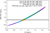 |
Fig. 4. Strong parameter correlation (Torres et al. 2000) between light ratio lB/lA and radius ratio for TESS and SAT data. The horizontal lines show the spectroscopic light ratio for the TESS passband and its uncertainty. |
In addition to the seven basic light curve model parameters, additional parameters and their statistical significance were systematically tested for. RV data were not included at this stage. We tested for: one- and two-parameter LD laws (with coefficients fixed / free), orbital eccentricity (e cos ω and e sin ω), and third-light (l3). Model selection is based on a standard hypothesis test invoking the Fisher-Snedecor ℱ-statistic (Lucy & Sweeney 1971) and is akin to a analysis-of-variance (ANOVA) test. At each testing stage, when including a new parameter, we tested for the rejection of the null-hypothesis at a 0.1% significance level. This was done for each additional parameter sequentially. The parameter that passed the hypothesis test while simultaneously resulting in a maximum improvement (Δχ2) to the model fit, was then included consecutively replacing the previous model with an extended model. The testing sequence was then repeated for all remaining parameters.
We found that the data support the detection of limb-darkening. The next best improvement in the χ2 statistic was found by including a quadratic limb-darkening law. We do not see any statistical evidence for the SAT data to support a detection of the e cos ω eccentricity term either after the ℱ-test based model comparison.
An additional consideration examined whether spots during eclipses could be accounted for with the application of a polynomial trend removal (invoking the poly option in JKTEBOP), we calculated k with and without detrending while considering parameter uncertainties from TASK8 and TASK9. We found differences at the 0.70σ (TASK8) and 1.1σ (TASK9) levels. We conclude that imposing any attempt of detrending the eclipses does not improve the measurement of k.
We decide to only retain a quadratic limb-darkening law with coefficients obtained from the LIMBDARK17 code. Uncertainties were obtained from proper error propagation by fixing k − δk, k and k + δk in turn. We scaled data errors to force the reduced χ2 = 1.0. Final SAT light curve parameters are presented in Table 5. We note that the best-fit LD coefficients are not to be trusted and are poorly constrained by the data. Plots of best-fit models in each SAT band are shown in Fig. 5.
Best-fit photometric parameters for SAT uvby bands.
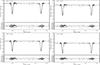 |
Fig. 5. Strömgren (SAT) uvby light curves of NY Hya. We show data from the 97/98 and the 98/99 season. The solid line shows the best-fit model obtained from JKTEBOP. The residuals are shown below each model fit. |
The code allows the simultaneous fitting of RV data (Southworth 2013). The five parameters are the semi-amplitudes KA, KB, eccentricity e, argument of pericentre ω and the systemic velocity γ. Instead of fitting for e and ω individually, the code fits for e cos ω and e sin ω to break a strong correlation between e and ω (Pavlovski et al. 2009). In the code, the parameters e cos ω, e sin ω, T0 and P are constrained simultaneously by photometric and spectroscopic data. The inclusion of RV data can result in a significant improvement in the photometric measurement of e sin ω (Wilson 1979). As described in Southworth (2013), JKTEBOP allows the two stars to have different systemic velocities, γA and γB, in order to detect any possible systematic effects in RVs due to discrepancies between the FEROS spectra and a chosen template spectrum. We fitted for γA and γB and found a negligible difference at the 0.28σ level. This result is consistent with and as expected for two near-identical stars. Therefore, we fitted for a single systemic velocity. Finally, we did not perform a ℱ-test on RV parameters and assume that the above model is a correct description of spectroscopic data.
5.2. TESS photometry
We also analyzed the TESS short-cadence data (13420 data points) since this is the most precise data potentially providing tighter constraints on model parameters as compared to the SAT data. We included all times of minimum light from the SAT 97/98 and 98/99 eclipses as an additional observational constraint on the ephemeris. The largest difference in residuals between SAT data and the ephemeris was found to be 1.2σ. TESS SC data posits no danger for light curve smearing effects (Southworth 2011). TESS flux units and associated uncertainties were converted to magnitudes. The out-of-eclipse baseline magnitude was detrended and normalised with a cubic spline function. Finally, we iteratively removed outliers that are present in the TESS photometry by rejecting data points lying greater than 3σ from the best fit. We tested for any differences (considering rA) for a 4σ clipping and found none.
We investigated the effect of various LD laws (linear, logarithmic, quadratic and square-root) on the fractional radii (rA, rB). We find no evidence for any systematic errors with a maximum difference at the 0.02σ level. Third light was not detected at a significant level within the TESS aperture mask. This result is consistent with the high-resolution Lucky-Imaging observations as well as non-detection of third-light in FEROS spectra indicating the non-detection of stellar companions. As a result, we found that accounting for the limb darkening through the square-root law and the addition of geometric parameter e cos ω improved the success of the fits for a 10-parameter model statistically significantly. The non-zero eccentricity cannot be explained by the light-travel time effect because the mass ratio for the two components is very close to unity. Also, no apsidal motion is expected for a circular orbit. The RMS scatter for this 10-parameter model was found to be significantly larger than the mean value of photometric error returned by the LIGHTKURVE pipeline. We therefore conclude that the original TESS error bars are underestimated and likely account only for Poisson counting statistics per point. Although we tested with the geometric parameter e sin ω from the pool of parameters, TESS data do not support the inclusion of e sin ω (or any other parameter that was tested for in the sequence) beyond what was found. Finally, we note that the ℱ-test is consistent with the general finding that e sin ω is less constrained than e cos ω (Kallrath & Milone 2009; Southworth 2013). Surprisingly, this is also the case for the high-precision TESS data presented in this work.
For partial eclipses, the ratio of the radii becomes strongly correlated with orbital inclination and surface brightness ratio which implies that the light ratio becomes strongly correlated as well with the ratio of radii. We therefore added a spectroscopic light ratio from FEROS in the TESS passband (lB/lA = 1.149 ± 0.035) as an additional constraint on the light curve model (Andersen et al. 1990; Torres et al. 2000; Southworth et al. 2007). In Fig. 4, we show the results of including and not including a spectroscopic light ratio for TESS data. The difference in photometric and spectroscopic light ratio was found at a 0.41σ level. However, final parameters have been obtained by adopting and fixing k ± δk from the SAT y band constrained with a spectroscopic light ratio which is much more accurately determined due to the narrower passband compared to the TESS filter. The final modelling included times of minimum light from TESS as an additional observational constraint on the ephemeris.
5.3. Final solution and parameter uncertainties
We fitted clipped TESS data with RVs simultaneously. Although TESS is a space-based observing platform we cannot rule out instrument-related correlated noise (pixel-to-pixel variations, temperature fluctuations, etc) or correlated noise of astrophysical nature (star spots) that are not accounted for in the modelling process. We therefore inferred parameter uncertainties from running the classic bootstrap (TASK7), Monte Carlo (TASK8, MC) as well as the Residual-Permutation Prayer-Bead (TASK9, RP-PB) algorithms within JKTEBOP. As a test we ran 5000 and 10 000 trials for TASK7 and TASK8 and found no difference.
For the TESS data, we found that the nominal photometric errors as returned by LIGHTKURVE were underestimated by a factor of roughly 1.6 based on the inherent data scatter. Therefore, for the final uncertainty estimation the input errors were scaled by  to force the reduced χ2 = 1.0. The scaling relies on several assumptions (Andrae 2010): i) errors follow a Gaussian distribution, ii) the model is linear in all parameters and iii) the applied model is a correct description of the data. In Fig. 6, we show the best-fit model and Table 6 lists the final best-fit parameters. We did not detect any skewness in the resulting parameter parent distributions for each algorithm and thus report a symmetric 1σ uncertainty. Parameter uncertainty covariances and parameter parent distributions for light curve and RV data are shown in Figs. C.1 and C.2. We found the PB-RP algorithm to yield the largest uncertainty for most parameters and refer to Table 6 for details. In general, we adopt and report the largest uncertainty for a conservative estimate and refer to Turner et al. (2016) for a discussion on realistic uncertainties.
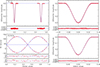 |
Fig. 6. Result of simultaneous JKTEBOP fitting of NY Hya. Observational data are shown in red and best-fit models as solid lines. No error bars are plotted. Left column: TESS light curve (top) and FEROS RV curves (bottom). Right column: details of the primary (top) and secondary (bottom) eclipse clearly showing the presence of time-correlated red noise in the residuals. |
Best-fit parameters to the TESS and FEROS data for fixed values of k as obtained from SAT y band data with proper error propagation.
Finally, we performed a quantitative auto-correlation test on the residuals of photometric and RV data. This test aims to detect any non-random structure or systematics in the residuals indicating a deviation from a standard normal distribution. For this, we calculated the Durbin-Watson (𝒟) statistic (Hughes & Hase 2010) for each data set and found 𝒟 = 0.95, 2.47 and 1.41 for the TESS, RV (star A) and RV (star B) data sets, respectively. We show the resulting DW lag plots in Fig. 7. Relatively, the auto-correlation in the TESS data is stronger compared to the two spectroscopic data sets. This result quantitatively confirms the presence of systematic noise in the TESS data most prominently seen during primary and secondary eclipses.
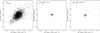 |
Fig. 7. Durbin-Watson (lag) plots for the three different data sets: TESS, RVs of star A, and RVs of star B. A 𝒟 = 2.0 indicates no auto-correlation with data randomly distributed following a standard normal distribution. For the TESS data and the RV data of star B (based on two outliers) we see a positive auto-correlation, while for the RVs of star A we see a negative auto-correlation. |
6. Physical properites
6.1. Spectral disentangling
In order to disentangle our spectra and obtain a single spectrum for each of the components, we first performed a preliminary fit to our RV measurements with TODCOR by making use of the IDL code RVFIT.PRO (Iglesias-Marzoa et al. 2015), and derived a preliminary set of orbital parameters for the system, which turned out to be in good agreement with the results from JKTEBOP presented in Table 6 and hence support our findings from the simultaneous modelling of light and radial velocity curves. We made use of the FDBINARY code (Ver. 3.0; Ilijic et al. 2004) to disentangle our continuum-normalised, composite spectra of NY Hya. We converted the wavelength axis of the spectra to logarithmic units and sampled each spectrum equidistantly by making use of cubic spline interpolation. We assigned the orbital phases computed from the linear ephemeris in Eq. (1) to each of the processed input spectra. We made use of four of the orbital elements (eccentricity, the longitude of the periastron and semi-amplitudes) which we derived from our preliminary RV fit. Since we did not detect a phase shift or apsidal motion in the system, we have fixed the relevant parameters to zero. We set the number of optimisation runs to 1000 and the number of iterations to 10 000.
Spectral disentangling is performed in Fourier space using the Keplerian RVs based on five orbital parameters by FDBINARY. Light ratios form an optional parameter set. We experimented using the light ratios we derived from TODCOR as well as adjusting them (fixing its value to one for each input spectrum). We had very similar results in both attempts in terms of the quality (expressed with the S/N) and depths of the spectral lines. The code outputs the disentangled spectra as well as the residuals (O − C) and the RVs. We compared the RVs computed by FDBINARY with that from other independent methods and assessed its results as consistent with the others.
6.2. Stellar atmospheric parameters
The SED analysis, described in more detail in Sect. 7, provides an estimate for atmospheric parameters of the system. Therefore, we decided to make use of the synthetic spectrum fitting technique with these estimates (Valenti & Fischer 2005), better suited to estimate the Teff of stars with heavy line blending, which becomes an important problem in the spectral analysis of stars on the cooler side of 5500 K. Since other methods heavily rely on EWs of individual lines and their ratios, they are not deemed to be optimum to extract stellar atmospheric parameters (Tsantaki et al. 2013).
We used the latest version of ISPEC (Blanco-Cuaresma 2019) in order to derive the stellar atmospheric parameters of each component. We first corrected both of our disentangled spectra for the systemic velocity. We made use of the rough estimates for Teff (5550 and 5500 K, for star A and B respectively), log g (4.15 for both components), and [M/H] (solar abundance) as initial parameters. We experimented with different amounts of line broadening to determine an initial value for the projected rotational velocity (v sin i) by employing the template spectra we used in the measurement of the RVs with TODCOR for the purpose and determined a value of 15 km s−1. Since we expect the components to be tidally locked we assumed the same rotational velocity for both of the components. We used the SYNTH3 code (Kochukhov 2007) for computation, ATLAS9 (Castelli & Kurucz 2003) for the stellar atmosphere model, solar abundances from Asplund et al. (2009), and a modified version of the VALD line list in the wavelength ranges of our spectra (Piskunov et al. 1995).
We combined all disentangled spectra from four different wavelength regions to achieve a global fit consistent with all of them for both of the spectra separately. We then selected the entire combined spectra from four different wavelength regions with ISPEC to fit with the least-squares minimisation method. ISPEC also filters out the lines from its analysis for which a Gaussian fit fails. We then ran the code and had our first fits, which agreed mostly with the observed spectra. However, we had very large error bars in all parameters and significantly lower value (log gA ∼ 3.95 cgs) compared to that we have from the first light curve modelling attempts (log gA = 4.183, log gB = 4.188). Surface gravity is the least dominant factor in shaping the spectra of cool dwarfs. Therefore, it leads to significant degeneracies in the fitting procedure and large error bars in all the parameters. Since its effect is only marginal in synthetic spectrum fitting, it will be more adequate to determine log g from light- and RV curve analysis. Therefore, we fixed the surface gravity at log gA = 4.2059 for star A and log g = 4.210 for star B from their measured masses and radii. We found that fixing the parameters to these values significantly decreased the fitting uncertainties on other parameters. We provide the values of the atmospheric parameters for each of the components derived from modelling of the disentangled spectra in Table 7. In Figs. 8 and 9, we also provide two spectra for each of the components (star A at the top, star B at the bottom) from two different wavelength regions to illustrate the success of our models from the synthetic spectrum fitting.
Atmospheric parameters of the components in NY Hya.
 |
Fig. 8. Model and disentangled observed FEROS spectrum in the 4090–4140 Å region. Top panel: disentangled spectrum of star A (plus symbols) and its best model. Bottom panel: same content, but for star B. |
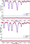 |
Fig. 9. Same as Fig. 8, but for the 5202–5214 Å region for star A (top panel) and star B (bottom panel). |
We attempted to estimate an age for the system by employing different techniques for the purpose. We found neither core-emission signals in the Hα line nor the signs of lithium absorption in the spectra recorded at convenient orbital phases for the job. We also employed the chromospheric activity indicators SHK and  determined as 0.37 and −4.5, respectively by Isaacson & Fischer (2010) from three low S/N (≃35 each) spectra they acquired at the orbital phases 0.65, 0.86 and 0.28 as a result of which they reported an age of 0.47 Gyr for NY Hya using calibration relations from Mamajek & Hillenbrand (2008). These measurements should only be regarded as an upper limit because any flux velocity-shifted out of the passband will cause this number to increase to more-active levels when the binarity is ignored. Applying the empirical X-ray activity based on the fractional X-ray luminosity (RX = LX/LBol) vs. age relation from Mamajek & Hillenbrand (2008), we derived an age of 0.19 Gyr. However, we defer the age determination to a comprehensive analysis of the system’s evolutionary history.
6.3. Interstellar extinction and reddening
Correcting for extinction is important to infer an accurate Teff estimate from broad- and intermediate-band photometry predominantly in the blue wavelength region. Following Mann et al. (2015) and Aumer & Binney (2009), the effect of extinction/reddening is essentially zero for stars within 70 pc due to a low-density cavity defining the ‘Local Bubble’ in the solar neighbourhood. This finding is consistent with Reis et al. (2011) and Bessell et al. (1998) suggesting that reddening may be ignored for stars within 100 pc (Perry et al. 1982). Therefore, towards the direction of NY Hya, galactic coordinates (l, b) = (239° ,29° ), a small and possibly negligible amount of extinction is expected at the measured distance of around 106 pc.
The reddening E(B − V) can be estimated from maps of galactic dust, based on which colour indices can be de-reddened and an interstellar extinction value (AV) can be derived. We made use of the dust maps provided by Schlegel et al. (1998), Schlafly & Finkbeiner (2011), Green et al. (2014, 2018), Lallement et al. (2014) and Capitanio et al. (2017) to estimate the reddening value. In that regard, as pointed out by the referee, the Schlegel et al. (1998) and Schlafly & Finkbeiner (2011) dust maps18 estimate the total reddening towards the direction of NY Hya to infinity. When making use of the NASA/IPAC service no distance information is provided. This approach would overestimate the reddening for NY Hya. Reddening/extinction at the distance of NY Hya is given by the ARGONAUT19 (Green et al. 2014, 2018) and STILISM20 (Lallement et al. 2014; Capitanio et al. 2017) tools. Both projects yielded a reddening consistent with zero. From ARGONAUT we found  mag. From STILISM we found E(B − V) = 0.0030 ± 0.015 mag. Formally, the resulting (conservative) weighted mean for the reddening at NY Hya is E(B − V) = 0.0065 ± 0.025 mag (consistent with zero) and was adopted in subsequent calculations. Reddening values for HD 82074, HD 80446 and HD 80633 were found using STILISM.
We then de-reddened the SAT Strömgren colour indices using the reddening relations given by Crawford (1975) and Crawford & Mandwewala (1976). The colour excess for the (b − y) colour is given as E(b − y) = 0.74E(B − V) (Crawford 1975). The remaining (updated) relations are found from Crawford & Mandwewala (1976) which were also applied by Casagrande et al. (2011) and are valid for stars covering a wide range of spectral types including late-type F-, G- and M-dwarfs. In particular, the relations E(m1) = (−0.3333 ± 0.0051)E(b − y), E(c1) = (0.1871 ± 0.0071)E(b − y) were implemented in the IDL21 routine DEREDD.PRO and applied in Southworth et al. (2004b). In Table 8, we quote the reddening-free colour indices. Uncertainties were obtained from Monte Carlo simulations assuming Gaussian errors.
Extinction-corrected Johnson V magnitude (from extinction law) and de-reddened Strömgren colour indices for NY Hya and (constant) check stars.
We calculated the interstellar extinction using the extinction laws AV = (3.14 ± 0.10)E(B − V) Schultz & Wiemer (1975), Fitzpatrick (1999) and AV = (4.273 ± 0.012)E(b − y) (Crawford & Mandwewala 1976). We find very good agreements between the various methods at a 0.05σ level. In Table 8, we quote the extinction-free Johnson V magnitudes for NY Hya and comparison/check stars. We quote the value obtained from the extinction law. Uncertainties were also obtained from Monte Carlo simulations assuming Gaussian errors.
In addition, the colour excess E can be calculated via intrinsic colour calibration relations based on Strömgren uvby − β photometry. We checked the range of validity of two calibration relations (Schuster & Nissen 1989; Karataş & Schuster 2010) for thexs measured colour indices and β value measured for NY Hya, both of which are valid for late F- to G-dwarfs. We find good agreement ( < 1σ) between the values we found based on both calibrations and also with our previous estimates presented in Table 8. In conclusion, the colour excess estimates indicate a very small amount of reddening with E(b − y) nearly being consistent with zero. This implies that interstellar absorption/scattering is small at the direction and distance of NY Hya.
7. Spectral energy distribution modelling
We compiled archive broad-band (reddened) photometry covering the wavelength range from far-ultraviolet to mid-infrared to determine a SED model for NY Hya as a single star. The near-identical nature of the two stars justifies this and provides a unique opportunity to determine a relatively accurate estimate of atmospheric properties. The Teff is most reliable since the broad-band photometry aims at measuring the flux continuum and therefore probes various slopes of the SED depending on wavelength. We assume that the archive photometry data regards NY Hya as a single star. The resulting Teff will be a mean value which will be close to the true values for each star. The derived flux will be overestimated by a factor of two. We first present some details of photometric sky surveys relevant for NY Hya.
7.1. Broad-band photometry
We obtained broad-band magnitudes of NY Hya from different photometric archives. Strömgren uvby magnitudes can be reconstructed from Strömgren colour indices (b − y),m1, c1 and from assuming Johnson V equals Strömgren y. This assumption is valid since the two filter transmission profiles are near-identical (with V more broader than y) and generally there are no strong features in the V bandpass. Furthermore, the transformation from the instrumental Strömgren y (yinstr) to the standard Johnson V, based on a large number of bright standard stars, is of the form V = A + B(b − y)st + yinstr (Crawford & Barnes 1970), where the coefficient B is around 0.02. Since (b − y)st varies from about 0.000 for an A0V star to about 0.500 for a K1V star, the difference between Johnson V and yinstr for most of the here relevant part of the main-sequence stars is between 0.000 and 0.010 mag (apart from the arbitrary zero point A). On nearly all 63 nights, the number of bright standard stars was sufficient to ensure a correct transformation of yinstr to Johnson V.
As noted earlier, Paunzen (2015) provides Strömgren data for NY Hya in his catalogue, but we deem those measurements not trustworthy. Standard Strömgren magnitudes are given as


where the associated 1σ uncertainties are found from standard error propagation, assuming no correlations between uncertainties and independent variables and are given as
We have implemented the above equations and numerically propagated errors via Monte Carlo simulations and can confirm the validity of the expressions in uncertainties. We used the V band estimate and Strömgren colour indices at phase 0.25 (cf. Table 1). However, we find that the u and v band estimates are systematically deviating > 10σ in all our SED models. We have therefore not included those points.
We also decided to discard the DENIS22 (Deep Near Infrared Survey of the Southern Sky; Paturel et al. 2003) I, J, KS photometry, since the DENIS Johnson J (1.25 μm) and KS (2.16 μm) magnitudes are nearly identical to the 2MASS (Skrutskie et al. 2006) photometry. Given the higher 2MASS photometric precision (indicated by good survey quality flags), we chose to only retain the 2MASS data. 2MASS JHKS observations were taken at epoch JD 2 451 199.8029. This corresponds to an orbital phase of 0.17 for NY Hya and hence reflects an out-of-eclipse brightness in each passband. We also ignored the SkyMapper data recorded in similar passbands ((u, v, g, r, i, z)) to other all-sky surveys because they are based on fewer images, even though they are recorded during out-of-eclipse phases.
We have retrieved raw data from APASS (American Association of Variable Star Observers Photometric All Sky Survey; Henden et al. 2015) via the URAT1 (US Naval Observatory Robotic Astrometric Telescope; Zacharias et al. 2015) catalogue. While the original APASS (DR9) archive does not provide a Sloan i-band magnitude and measurement uncertainties in all five APASS passbands, the URAT1 catalogue does. However, the data reported in the URAT1 catalogue does not match the APASS (DR9) catalogue listings. We therefore obtained unpublished photometry, which were acquired at times outside eclipses, following a conversation with A. Henden, and calculated their average values and standard deviations for each filter. Comparing APASS VJ with Strömgren y and Tycho-2 VT, we find good agreement and use them in the SED modelling as provided in Table 9.
Compiled archive photometric measurements of NY Hya.
All Pan-STARRS (Chambers et al. 2016; Flewelling et al. 2020) data have been included in our analysis except for the iP1 point which we found to deviate by > 10σ for all our SED models and hence seem unreliable.
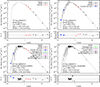 |
Fig. 10. VOSA SED model fits (corrected for extinction) for various data sets of flux measurements for NY Hya. The horizontal lines in the residual plots mark ±3σ deviation from the model. Panel A: WISE and 2MASS flux measurements |


The recently published Gaia DR2 data (GBP, G, GRP, Gaia Collaboration 2018) were included in our SED analysis too. We converted the calibrated flux into magnitudes using the revised zero-points for each pass-band. Uncertainties were propagated via Monte Carlo simulations. The resulting distribution in magnitude-space was found to be near-Gaussian. The median value and 68% confidence interval (±1σ) was determined to infer uncertainties in the three magnitudes.
7.2. SED modelling
We utilised the Virtual Observatory SED Analysis (VOSA23 Ver. 6.0) online tool (Bayo et al. 2008). VOSA derives stellar properties using theoretical atmosphere models from which synthetic fluxes are calculated to fit observations of NY Hya. All archival photometry has been compiled in Table 9. Astrophysical constants follow the IAU 2015 Resolution B3 recommendation for Solar values (Prša et al. 2016). All archival photometry is corrected for extinction using R = 3.14 and E(B − V) = 0.0065 mag (see the previous section), thus avoiding a possible underestimation of the Teff. We also provided a Gaia DR2 parallax to VOSA allowing a semi-empirical estimate of the total flux emitted and derived stellar radius.
The five SED model parameters are Teff, surface gravity (log g), metallicity ([m/H]), extinction (AV; by providing R = 3.14 and E(B − V) = 0.0065 mag) and a flux density proportionality factor (Md) to scale the theoretical spectrum to observed fluxes. The surface gravity and metallicity are generally poorly constrained from broad-band photometry and are therefore the least accurate quantities. The reduced χ2 statistic ( ) is used to assess the quality of the fit. As a rule of thumb (C. Rodriges, priv. comm.) reasonable accurate SED models have
  < 50. Errors were found from a Monte Carlo bootstrapping algorithm and are mainly limited by the parameter grid mesh for a given atmosphere model. We searched for best-fit models from the following atmosphere models: KURUCZ (Castelli & Kurucz 2003), COELHO (Coelho 2014) and a suite of PHOENIX24 (Allard et al. 1994, 2012) models: BT-NEXTGEN-GNS93, BT-NEXTGEN-AGSS2009, BT-SETTL BT-COND, BT-DUSTY: (Allard et al. 2012), BT-SETTL-CIFIST (Baraffe et al. 2015), NEXTGEN (Hauschildt et al. 1999). No parameter limits were chosen a priori.
In Table 10 we list the first few best-fit models in order of increasing  ; the first model is shown in Fig. 10C. We note that SED models with an outdated solar composition (Grevesse & Noels 1993; Grevesse & Sauval 1998) tend to systematically yield lower Teff by about 200 K compared to atmosphere models adopting more recent (Grevesse et al. 2007; Asplund et al. 2009; Caffau et al. 2009) solar abundances. Considering the formal uncertainties in Teff, this difference between the competing models is significant. In Fig. 10, we show four different SED models considering various data sets. Formally, the best-fit model yields a temperature of Teff = 5700 K, which agrees with the Gaia (Gaia Collaboration 2018) mean estimate to within 1.7σ although the SED uncertainties of 50 K is generally judged to be likely too optimistic by community members. To obtain an idea of a realistic uncertainty, we refer to the VOSA documentation where the modelling performance was investigated by comparing model estimates with high-quality Teff estimates of FGK stars from the ELODIE V3.1 (Prugniel et al. 2007) catalogue. The catalogue was cross-matched with the Gaia EDR3 catalogue retaining stars with a parallax > 10 mas to avoid extinction. For a statistically large sample and considering the BT-SETTL-AGSS2007 and KURUCZ models, mean differences in the range 6–50 K were determined. From this, we conclude that the uncertainties in Teff in Table 10 seem to be realistic given that NY Hya has a parallax of π = 9.4 mas.
7.3. Physical properties and photometric distance
Final physical properties of NY Hya were calculated using JKTABSDIM25 (Southworth et al. 2005a, Ver. 15) from the measured values P, rA, rB, i, e, KA and KB. Consistency is ensured by implementing the IAU 2012/2015 Resolution B2/B3 (Prša et al. 2016) for Solar values. Proper error propagation is performed and we list final values in Table 11.
Physical properties of the two components in NY Hya as derived from TESS photometry and FEROS spectral data.
Tidal interactions in binary star systems will have effects on both stellar rotation and orbital (mainly eccentricity) evolution (Torres et al. 2010). For the measured orbital period and mass-ratio the turbulent dissipation and radiative damping formalism by Zahn (1977, 1989) predicts a (e-folding) synchronisation timescale of 5.2 Myr and a (e-folding) timescale for orbit circularisation of 1.3 Gyr. We found the orbit of NY Hya to be near-circular. However, an indication of system age is obtained only if the initial orbital eccentricity is known. A circular orbit does not necessarily imply an old system. As an example, the V615 Per system has a circular orbit even though the period is relatively long (13.7 d) and the system is only ≈20 Myr old (Southworth et al. 2004a).
From the measured radii and orbital period, we find the stellar equatorial rotation velocities to be 14.91 ± 0.16 km s−1 and 14.90 ± 0.18 km s−1 for star A and star B, respectively. The spectroscopic rotational velocities were found to be 15.77 ± 1.34 km s−1 and 15.71 ± 1.35 km s−1 and agree with the synchronous speeds to within 0.64σ. From this, we conclude that the system is tidally locked in a 1:1 spin-orbit resonance. This finding is in agreement with the period analysis of the TESS flux variation out of the eclipses from which we independently concluded that the system is rotationally synchronised.
Finally, we carried out a consistency check and calculated a semi-empirical distance from photometry and Teff. The photometric distance to NY Hya is computed from the surface brightness relations (Southworth et al. 2005a) adopting the empirical calibrations from Kervella et al. (2004) valid for dwarf stars between spectral types A0 and M2. We adopt the spectroscopic Teff measurements presented in Sect. 6.2 along with the 2MASS (Skrutskie et al. 2006) standard JHKS magnitudes and the Strömgren (SAT) derived Johnson V magnitude. We adopted the interstellar reddening E(B − V) = 0.0065 ± 0.025 mag from Sect. 6.3 to align the distances found in the various passbands. Having experimented with different passband magnitudes, which disagreed with each other slightly but provided photometric distances between 100 and 104 pc, we report a final photometric distance of 104.1 ± 1.5 pc from the 2MASS KS band (Kervella et al. 2004) since this measurement is affected least from uncertainties in interstellar reddening effects. This KS-band distance agrees with the astrometric Gaia DR2 measurement (106.10 ± 0.70 pc) to within 1.3σ.
7.4. Atmospheric properties from empirical relations
The SAT data provide an opportunity for consistency checks on the atmospheric properties from empirical calibration relations based on Strömgren colours. For a short review, we refer to Árnadóttir et al. (2010). We have made use of the UVBYSPLIT26 code with proper error propagation. The light ratios in the uvby passbands allow the derivation of Strömgren colours for each component star. Several calibration relations for Teff, log g and [Fe/H] exist. In all cases, we checked the validity of each calibration relation. Uncertainties in the colour indices were propagated via Monte Carlo simulations assuming Gaussian errors. The uncertainty from the calibration relation was added in quadrature to obtain the final uncertainty. This assumes no correlations between uncertainties. Important to note is that all calibration relations are based on FGK dwarfs (more or less). The work in Árnadóttir et al. (2010) offers some methodology to distinguish between dwarf and (sub-)giant stars. Based on the measured surface gravities, the two components in NY Hya are likely dwarf stars still on the main-sequence.
Olsen (1984) provides a calibration relation (Eq. (14)) for the metallicity based on standard relations for de-reddened colour indices (Árnadóttir et al. 2010; Torres et al. 2014). We find [Fe/H]A = 0.17 ± 0.18 dex and [Fe/H]B = 0.15 ± 0.18 dex. These estimates, albeit low precision, are consistent with solar metallicity. Metallicity estimates with high fractional uncertainties are obtained from Casagrande et al. (2011) and Holmberg et al. (2007) using calibration relations with de-reddened Strömgren colour indices. We find [Fe/H]A = 0.06 ± 0.39 dex and [Fe/H]B = 0.14 ± 0.38 dex (Holmberg et al. 2007) and [Fe/H]A = 0.17 ± 0.40 dex and [Fe/H]B = 0.23 ± 0.39 dex (Casagrande et al. 2011). Again, these estimates are consistent with a solar metallicity as was also determined from disentangled FEROS spectra.
Teffs are obtained from various sources and some relations (Holmberg et al. 2007; Casagrande et al. 2011) depend on metallicity. For solar metallicity, we find Teff, A = 5561 ± 196 K and Teff, B = 5591 ± 193 K (Alonso et al. 1996, Eq. (9)), Teff, A = 5637 ± 179 K and Teff, B = 5669 ± 172 K (Holmberg et al. 2007, Eq. (2), p. 522 considering 0.33 < (b − y) < 0.50), Teff, A = 5672 ± 181 K and Teff, B = 5705 ± 175 K (Casagrande et al. 2011) where we have added 20 K in quadrature as an additional uncertainty in the zero-point of the temperature scale (see their Table 4). For all these relations, we find an increase/decrease in Teff of 30–40 K when [Fe/H] is increased/decreased by 0.10 dex. An unpublished Teff − (b − y)0 calibration relation is obtained from Mamajek (2014)27. This relation is independent of metallicity. However, the median and 68.3% confidence interval for the metallicity of stars in the sample was found to be 0.0 ± 0.2 dex. We find Teff, A = 5648 ± 197 K and Teff, B = 5675 ± 194 K. Finally, Alonso et al. (1996) provide a calibration relation in the infrared based on TCS J − K colour and thus less affected by interstellar reddening. We find a mean temperature of ⟨Teff⟩ = 5673 ± 235 K. In general, we find good agreement with measurements obtained from FEROS data.
Several survey studies included NY Hya in their spectroscopic monitoring programs providing estimates of atmospheric properties. However, all these studies assumed NY Hya to be a single star. Measurements of stellar metallicity, surface gravity, and rotational velocity are all highly likely to be in error. The only quantity with some accuracy from these surveys is the Teff. As will later be argued, the two components in NY Hya are almost identical. Hence various measurements of Teff would represent a mean value not far from the actual value for each star. The works (no uncertainties were quoted) in Nordström et al. (2004), Holmberg et al. (2007) and Holmberg et al. (2009) report the same Teff = 5458 K and Robinson et al. (2007), McDonald et al. (2012) report 5678 K and 5719 K, respectively. We find a literature mean value of 5618 K for NY Hya as a single star. Assuming an uncertainty of 100 K this estimate is in good agreement (1.3σ) with a detailed spectroscopic analysis presented later in this work and also agrees (0.23σ) well with the Gaia (Gaia Collaboration 2018) estimate of 5647 ± 76 K. Gáspár et al. (2016) reports a stellar metallicity of [Fe/H] = 0.16 ± 0.06 dex, but this measurement does not account for binarity as well. Analysing double stars as single stars can introduce a significant bias in the metallicity estimate.
8. Stellar activity
We performed a period analysis on the three data sets, (SAT 97/98, SAT 98/99 and TESS). We applied PERIOD0428 (Lenz & Breger 2005). This package implements the Discrete Fourier Transform (DFT) algorithm (Press et al. 1992) and is suitable for the detection of periods in unevenly sampled time series data. In all three data sets, we removed all eclipses from the original data.
For the SAT 97/98 season, we show the results in Fig. 11 based on the Strömgren y-band light curve. The first panel shows the out-of-eclipse variability when all eclipses are removed. The second panel shows the spectral power for frequencies up to 50 cycles per day (c/d). No significant spectral power is found beyond this limit. Because of irregular sampling the Nyquist frequency of νNy ≈ 123 c/d was computed iteratively as the expectation value by means of a histogram analysis, based on recursive nested intervals (see p. 11 in Lenz 2005).
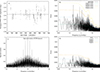 |
Fig. 11. Results of the period analysis for the SAT 97/98 y-band data set. Panel A: 404 y out-of-eclipse photometry showing magnitude vs. time where the primary and secondary eclipses have been removed. The horizontal line is the mean flux out of the eclipses as determined by PERIOD04 and was subtracted prior to the computation of the Fourier spectrum. Panel B: power spectrum and 1, 2, and 3σ noise levels. A frequency at f1 = 0.2138 c/d is detected corresponding to a period of 4.68 days. Frequencies near 1 c/d are likely daily/nightly alias frequencies. Panel C: power spectrum of the spectral (data gap structure) window. Panel D: power spectrum after removing the f1 frequency component with the highest power. Panels B and D have the same scale along the y-axis. |
In Fig. 11B the power spectrum of the recorded data shows several significant frequencies. We quantify the significance of a given frequency by calculating the 1σ, 2σ and 3σ noise levels as implemented within PERIOD04. We used the recommended (see p. 14 in Lenz 2005) stepping rate of 1/20T where T is the observational baseline time period (approximately 150 days). We determined a frequency with maximum power at f1 = 0.21381 ± 0.00018 c/d corresponding to a period of around 4.68 days. The best-fit amplitude and phase is of no interest and was omitted here. The uncertainty in frequency was obtained using the PERIOD04 built-in bootstrapping error estimation function. We chose 5000 Monte Carlo simulations. This result indicates that at least one component in NY Hya is contributing to a periodic modulation of the flux at the orbital phases out of the eclipses. To determine whether the remaining detected frequencies are real or spurious we pre-whitened the original power spectrum, as a result of which we ended up with one that resembles the noise level of the original power spectrum indicating that no further frequencies are to be found within the original data set.
The power spectrum of the out-of-eclipse fluxes for the SAT 98/99 data contains more information since the observation cadence was increased. We applied the same Fourier analysis methodology as for the 97/98 data set. The mean Nyquist frequency νNy was found to be around 199 c/d. A frequency of f1 = 0.20414 ± 0.00031 c/d was found at the 3σ noise level. This corresponds to a period of around 4.89 days and differs from the SAT 97/98 f1 frequency by 27σ. This result indicates that the out-of-eclipse variability is not constant suggesting a complex variation. The pre-whitened power spectrum still shows a number of frequencies although at a smaller significance (around 2.5σ) level. The highest frequency was found at f2 = 0.42824 ± 0.00018 c/d and corresponds to a period of around 2.35 days. This period is close to half the orbital period of NY Hya. This result suggests that the SAT 97/98 data set now contains a flux modulation out of eclipses at a period comparable to 1/1 and 1/2 of the binary period. The decrease in power for the f2 frequency corresponds roughly to around 0.5σ and hence the significance of f1 and f2 are somewhat comparable. Pre-whitening the original power spectrum with both f1 and f2 results in a power spectrum with no significant (beyond 2σ) frequency content (between 0.1 and 5 c/d).
The TESS data offer the potential for the most detailed period analysis due to the relatively high sampling cadence and photometric precision. We first phase folded the complete TESS data with the orbital period of NY Hya (4.77 days). The result is shown in Fig. 12. The observations clearly show photospheric flux changes at phases around 0.30–0.35 and 0.80–0.85 and hence are separated in time by approximately half an orbital period. The flux changes at phase 0.30–0.35 seem to change from orbit to orbit while the flux change at phase 0.80–0.85 are more or less constant. If these changes are caused by photospheric spot evolution, then the TESS data provides strong evidence for the presence of at least two spot features (during the TESS sector 8 time window) on either one or both components. Qualitatively, the spot at phase 0.30–0.35 changes in both flux (low temperature) and longitude/latitude position as the phase of minimum flux is changing. The spot feature at phase 0.80–0.85 is clearly larger spanning a longer phase period and also significantly hotter compared to the previous spot feature. We also see TESS systematics as discussed earlier, but their presence does not alter the spot evolution interpretation. Assuming synchronous rotation (see Sect. 7.3 for an argument to render this assumption true), the flux feature at phase 0.30–0.35 could be a spot located on the inward-facing hemisphere of one component or a spot located on the outward-facing hemisphere of the other component rotating into the line of sight of the observer after primary eclipse at phase 0.0. A similar chain of reasoning applies for the flux feature at phase 0.80–0.85. Without additional evidence it is impossible to decide whether both features belong to a single component.
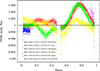 |
Fig. 12. Normalised TESS baseline flux (with eclipses) phases folded with the orbital period of NY Hya. The different colours encode successive times in the order black, red, green, blue, pink and yellow. |
We then computed a power spectrum from PERIOD04 using the complete flux data with TESS eclipses removed. The mean Nyquist frequency νNy was found to be around 359 c/d. As before, we have computed 1σ, 2σ and 3σ noise levels. As a ‘sanity check’, we have also computed a power spectrum using a PYTHON implementation of the LOMBSCARGLE algorithm (part of the ASTROPY29 package). The results were identical. We omitted the calculation of the False-Alarm-Probabilities (FAPs) from the LOMBSCARGLE algorithm as FAPs become less reliable for time series data with long data gaps (Reegen 2007). Following successive pre-whitening stages, the first five frequencies were found at f1 = 0.2029 ± 0.0014, f2 = 0.071 ± 0.011, f3 = 0.4180 ± 0.0012, f4 = 0.1055 ± 0.013 and f5 = 0.64 ± 0.31 c/d corresponding to periods of around 4.9, 14.1, 2.4, 9.5 and 1.6 days.
We conclude this section as follows. From the out-of-eclipse variability in TESS light curves, we have identified two clear increases in brightness after the 2nd and 4th eclipses. Assuming that these are the same feature seen twice, we get a rotational period of about 4.7 days. This was also inferred quantitatively from a period analysis where we detected a 4.7 and 4.9 day period when considering SAT 97/98 and TESS out-of-eclipse data, respectively. This is approximately the orbital period, but has been estimated from the stellar rotational modulation and not from orbital eclipses. We can interpret this as being indicative of at least one of the stars showing star-spot activity at the time of the TESS observations and that its rotation period is the same as the orbital period, i.e. the star has synchronous rotation. The synchronisation between the rotation of the components and the orbital period points towards a not very young system, with an age of at least few million years (see Sect. 7.3). Unless the stellar rotational velocities (v sin i) are significantly different (which they are not) it is not possible to work out which of the stars shows this spot activity. Evidence for photospheric activity via star-spot(s) is supported from spectroscopic observations. Several FEROS spectra exhibit clear Ca II K and H core emission lines (see Fig. 13) for each component which usually indicates photospheric activity.
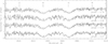 |
Fig. 13. Wavelength region around the Ca II K and H lines (3933.66 Å and 3968.47 Å) at different orbital phases. Core emission lines are visible for both components demonstrating chromospheric activity. The outermost vertical lines mark the location of the V and R continuum bands at 3901.07 Å and 4001.70 Å. |
From catalogue data, NY Hya appears to be active. This is supported by photometric data (Clausen et al. 2001) which shows out-of-eclipse variations in the Strömgren bands with an approximate 0.04 magnitude variability.
Smoking-gun evidence for stellar activity is found via the detection of significant X-ray emission with ROSAT and XMM-Newton. Szczygieł et al. (2008) used the ROSAT X-ray fluxes to determine a hardness ratio of 0.48 and estimate the system’s bolometric and X-ray luminosities. They found log(LX/LBol) = − 4.26 indicating a strong X-ray emission often associated with stellar youth as a first interpretation. They estimate a Rossby number of log(Prot/τconv) = − 0.51 assuming NY Hya to be a single star. Stellar activity was also reported by Isaacson & Fischer (2010) and Pace (2013) from spectroscopic observations measuring the core-emission component in the Ca II K and H lines. They reported  and Smax = 0.375, respectively, indicating a high level of chromospheric activity. However, these values should be treated with some caution since the binary nature of NY Hya might have shifted the Ca II lines away from their respective spectral windows used to define the
  index. No observational time stamps were provided by the authors to determine an orbital phase.
9. New Gaia astrometry and stellar kinematics
From the Gaia satellite (Gaia Collaboration 2018; DR2), the stellar parallax of NY Hya was measured to be π = 9.429 ± 0.062 mas (fractional uncertainty of σπ/π ≈ 0.0066). From d = 1/π and Monte Carlo error propagation, the median distance to NY Hya is found to be d = 106.10 ± 0.70 pc. The new Gaia parallax measurement is a significant improvement on the revised HIPPARCOS (Høg et al. 2000) measurement of π = 12.22 ± 1.16 mas (van Leeuwen 2007).
NY Hya has Gaia DR2 proper motion in RA and Dec measured to be μα cos δ = −60.06 ± 0.14 mas yr−1 and μδ = 48.16 ± 0.23 mas yr−1, respectively. The total on-sky proper motion is found to be 77 mas yr−1. This can be used to identify any unrelated background source. We compared the sky region towards NY Hya as observed by the Palomar Observatory Sky Survey (POSS I and II)30 providing archive imaging data from the 1950s. Since then around 70 yr have elapsed implying NY Hya to have moved around 5 arcsec on the sky. This is too small a displacement in order to be able to ‘look behind’ NY Hya, in an attempt to detect any unrelated background sources.
Combining the Gaia proper motion and distance results in a tangential velocity of 38.7 ± 0.27 km s−1. From modelling spectroscopic observations (see Sect. 3) the systemic RV to the binary barycentre was measured to be 40.79 ± 0.16 km s−1. By combining the total proper motion, distance and RV of NY Hya we find the galactic (J2000.0) 3D space position (X, Y, Z) = (−48.19 ± 0.32, −79.24 ± 0.52, 51.44 ± 0.34) pc and space velocity (U, V, W)LSR = ( − 41.90 ± 0.25, −3.01 ± 0.15, 18.21 ± 0.11) km s−1 relative to the local standard of rest (LSR), assuming a solar motion of (11.10, 12.24, 7.25) km s−1 from Schönrich et al. (2010).
The position and kinematics can be used to make inferences of the galactic population of NY Hya (Bensby et al. 2003; Soubiran et al. 2003) including an estimate of the system lifetime if identified with a stellar association. We applied GALPY31 and qualitatively searched the neighbourhood of NY Hya for any obvious cluster membership. A search out to a distance of 80 pc from NY Hya did not result in any obvious cluster membership. In the U − V space we found a small over-density of stars, but it is located more than ∼10 pc from NY Hya. We also applied the BANYAN-Σ (Gagné et al. 2018) code32 and found no cluster membership to any of the 27 known young associations within 150 pc. A probability of 99.9% of NY Hya being a field star was returned. Therefore, no obvious relationship to any star association was found, significantly diminishing the possibility of age determination via main-sequence fitting. We also calculated the membership probability of NY Hya belonging to the thin, thick or halo population (Reddy et al. 2006; Bensby et al. 2014). From Bensby et al. (2014), we find percentage probabilities of (Pthin, Pthick, Phalo) = (97.7, 2.3, < 0.1)% indicating that NY Hya belongs to the galactic thin disc population. Stellar ages for this population are in the range from 0 to 10 Gyr and thus the lifetime of NY Hya is unconstrained from 6D kinematical considerations.
10. Comparison with stellar evolution models
NY Hya is among a small number of bright detached eclipsing binary systems for which most relevant physical properties for the component stars are constrained by observations (masses, radii, temperatures, luminosities, metallicity; Torres et al. 2021). This allows for stringent tests of stellar structure and evolution model predictions, including models that incorporate non-standard physical ingredients (e.g. star spots, magnetic fields).
Comparisons with stellar structure and evolution models were performed using models from the Dartmouth series (Dotter et al. 2008; Feiden 2016). Models used in this analysis deviate from the original Dartmouth Stellar Evolution Program release (Dotter et al. 2008, DSEP) with changes that make them more suitable for studying M-dwarfs and pre-main-sequence (PMS) stars (see, e.g. Feiden 2016). There is also a difference in the adopted solar composition, with Feiden (2016) adopting a more recent solar Z/X value (Grevesse et al. 2007) compared to Dotter et al. (2008). Differences in fundamental stellar properties in the solar-mass regime are small owing to both model sets calibrating to the Sun. This calibration mitigates differences in model predictions owing to variations in the adopted physics and solar composition. The primary reason for choosing this model set was the ability to perform controlled numerical experiments by calculating standard and non-standard (e.g. magnetic, reduced αMLT) evolution models with otherwise consistent physics.
We used a grid of stellar model mass tracks and isochrones that are described in Feiden et al. (2021). For this work, the grid was extended to include masses between 0.8 M⊙ and 2.0 M⊙ with a grid spacing of 0.05 M⊙ above 1.0 M⊙. Metallicity values in the grid ranged between −0.7 ≤ [Fe/H] ≤ +0.5 with a spacing of 0.1 dex. Simple isochrones were computed for ages between 0.1 Myr and 10 Gyr with an age spacing approximately equal to 10% of the isochronal age (e.g. 0.1 Gyr for ages > 1 Gyr).
10.1. Model inference procedure
Testing the validity of stellar model predictions was done using three procedures: (1) an initial by-eye comparison, (2) estimating the most probable model properties for each component in NY Hya using a Markov Chain Monte Carlo (MCMC) method, and (3) individual modelling of the two components based on measured properties (cf. Table 11). The latter approach was only used for conducting controlled experiments using non-standard model physics (cf. Sect. 10.3).
By-eye relied on comparing a number of stellar model isochrones to the properties of NY Hya to establish an approximate model age and metallicity. The intention was to provide a check on the MCMC analysis and provide a baseline for performing controlled experiments with non-standard models, should they be needed. Results of the by-eye comparison were also used to set initial conditions in the MCMC algorithm (see below), though testing revealed the results were insensitive to this choice.
Posterior probability distributions (PPDs) for the inferred stellar evolution model properties were integrated using an MCMC method. We used emcee (Foreman-Mackey et al. 2013) to implement an affine-invariant ensemble sampling algorithm. Our likelihood function is the same as that used by Mann et al. (2015). This included a uniform prior distribution for the component ages, a choice that could be improved in the future to disfavour phases of rapid stellar evolution. The set of unknown parameters was taken to include the system age, system metallicity, and the two component masses. Each of these parameters has an associated prior probability distribution that helps constrain the permitted model results. These four parameters are required to specify a unique set of model properties (radius, luminosity, and temperature) for each component that are constrained by observations.
Our analysis used 100 walkers taking 1000 steps yielding a total of 100 000 random samples of the joint posterior probability distribution. We experimented with larger simulations containing 1000 walkers with 100 000 steps, but found the results were nearly identical to the smaller simulation. Each walker was seeded using a value for each unknown parameter drawn from a Gaussian distribution centred on the results of our initial by-eye comparison. Simulations seeding the walker with random values for each unknown parameter did not affect our results, but did require more steps for convergence. For each random realisation of the unknown system properties, a corresponding set of individual component properties were found by linearly interpolating within our grid of stellar model isochrones (see e.g. Mann et al. 2015; Feiden et al. 2021). The age sampling in our isochrone grid was fine enough that linear interpolation provided reliable results as long as the model stars were not ascending the red giant branch. Given the estimated log g for each star was greater than 4.0, our lack of resolution on the red giant branch was not a problem.
10.2. Standard models
Results from our initial by-eye comparison of NY Hya’s observed component properties to standard stellar models are shown in Figs. 14 and 15. Each figure plots three stellar model isochrones with different metallicities and ages that were found to best reproduce the observed data (filled points). Figure 14a demonstrates that finding agreement in the mass-radius plane can be accomplished using models of almost any metallicity. Predictions for the system age differ, with lower metallicity models producing younger ages. We find a predicted age of about 4.4 Gyr at solar metallicity, 5.7 Gyr when [Fe/H] = +0.20, and 7.3 Gyr with [Fe/H] = +0.40.
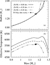 |
Fig. 14. Mass-radius (top panel) and mass-Teff (bottom panel) diagrams showing the components of NY Hya (solid points) against three standard Dartmouth stellar evolution models. The age-metallicity combinations of the isochrones are ([Fe/H], τage) = (+0.0, 4.4 Gyr; solid line), (+0.2, 5.7 Gyr; dashed line), and (+0.4, 7.3 Gyr; dash-dotted line). |
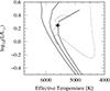 |
Fig. 15. Hertzsprung-Russell diagram showing the two components of NY Hya (solid points) against three standard Dartmouth stellar evolution model isochrones (solid lines) and a single stellar evolution model mass track (dotted line). Isochrones are shown with the same line style to provide contrast with the individual mass track. From left to right (warmer to cooler), the isochrones are ([Fe/H], τage) = (+0.0, 4.4 Gyr), (+0.2, 5.7 Gyr), and (+0.4, 7.3 Gyr). The stellar evolution mass track is showing an M = 1.160 M⊙ model with [Fe/H] = +0.4. |
To discriminate between models with different metallicities, we need information from the mass-Teff plane. Figure 14b shows that only super-solar metallicity models with [Fe/H] ∼ +0.40 are able to reproduce the observed Teffs from spectral synthesis (Teff ≈ 5600 K). This result disagrees significantly with estimates that the system has a near-solar metallicity. However, results from SED fitting did suggest a higher metallicity and high Teff (Teff, SED ≈ 5800 K) was plausible. In this case, super-solar metallicity models are still required to find agreement with the observed Teffs, with [Fe/H] ≈ +0.20.
To estimate uncertainties associated with our by-eye analysis and more rigorously explore the age-metallicity parameter space, we ran a series of MCMC simulations to estimate the joint posterior probability distribution for the model-predicted NY Hya properties. To constrain the system’s age, we first performed a comparison with standard stellar evolution models at a fixed metallicity, [Fe/H] = +0.00. Resulting PPDs for the system parameters were bimodal, suggesting NY Hya could either be a young, PMS system (τage ∼ 10 Myr) or an older main-sequence system (τage ∼ 5 Gyr). PPDs for the component masses and component radii were consistent within the 1σ uncertainty of the observations. However, model Teffs were inconsistent with the measured values in each case, similar to what was found in the by-eye analysis. Assuming a young 10 Myr age implied that model Teffs were about 700 K cooler than our measured Teffs. Conversely, assuming a main-sequence age implied model Teffs were about 700 K warmer than the measured values.
A second series of simulations relaxed the fixed-metallicity assumption to allow for any metallicity values available in the model grid. We applied a Gaussian prior probability distribution centred on the estimated value ([Fe/H] = 0.07 ± 0.1), but that only weakly constrained the simulation results. We did enforce that both stars should have the same age and metallicity, assuming that a single system age and metallicity should apply. The resulting PPDs for the system parameters were again bimodal, but with strong correlations between metallicity and age. Younger solutions (∼10 Myr) were predicted to be sub-solar in metallicity, while older ages (∼6 Gyr) were decidedly super-solar.
This result is not surprising given the results of our fixed-metallicity simulations. Solutions suggesting the system has a young age were found to be too cool compared to the observations, and the opposite was true for older age solutions. Lowering the metallicity increases stellar Teffs, while increasing the metallicity has a cooling effect. The joint PPDs from the variable-metallicity runs highlight this effect as the simulations attempt to balance the Teff offsets by offsetting the system metallicity.
The young sub-solar solution suggests the system has an age τage = 12 Myr with [Fe/H] = − 0.35 ± 0.09 dex. The measured properties of the individual components are largely reproduced within the 1σ observational uncertainties (see Table 11). However, the radius of star A is not well reproduced. The model solution predicts that NY Hya A is smaller than observed by about 2.7% (2.5σ). Despite this, the solution could be viable.
There are two main difficulties with a young, metal-poor solution. The first issue is that the PMS phase is rapid compared to the overall lifetime of the star. NY Hya is not definitively associated with a young group. Thus, the prior probability of NY Hya (a random field star system) being this young is relatively small. The second problem is that models predict a significant abundance of lithium for a star of this mass at 12 Myr, with A(Li) ≈ 3.3. This is a testable prediction. However, there are no clear Li absorption lines present in the spectra of NY Hya (cf. Sect. 6.2). With no observational evidence of youth, a PMS solution is unlikely.
Alternatively, the older, super-solar metallicity solution suggests the system has an age τage = 6.5 Gyr with [Fe/H]init = + 0.30 ± 0.07 dex. The measured masses and radii of the individual components are reproduced within 1σ of the measured values. Teffs predicted by models are too warm by about 100 K, placing them within about 1.5σ of the measured Teffs. While the initial metallicity is significantly higher than the solar metallicity estimate, gravitational settling and diffusion acting over the lifetime of the model star suggest the metallicity at the main-sequence turn-off is about 0.1 dex lower than the initial value. This appears to be a viable solution. While encouraging, the difficulty with an older super-solar metallicity solution is that both stars must be at or just older than their respective core hydrogen exhaustion ages. This solution is a priori unlikely.
The problem with the old age, super-solar metallicity solutions predicted from by-eye fitting and the MCMC integration is that the resulting models are found to be just at the start of a rapid phase of stellar evolution. This is illustrated in Fig. 15, where an individual model mass track for an M = 1.160 M⊙ star with [Fe/H] = +0.40 is shown as a dotted line. The stars in NY Hya are right at the nexus of the core hydrogen burning phase and a proceeding period of core contraction prior to the establishment of hydrogen shell burning, where the mass track increases in luminosity and Teff. This phase of evolution is brief (τ ∼ 0.26 Gyr) compared to the overall lifetime of the star (τ = 8.5 Gyr). While it is not unfathomable that both stars would be near the end of the core hydrogen burning phase, the a priori probability of finding a star at this critical phase is small. Further evidence is needed to definitively establish the evolutionary stage of NY Hya.
10.3. Non-standard models
A standard model solution that finds both stars on the main-sequence does not appear to exist without modifying the physical ingredients of the models. PMS and main-sequence turn-off solutions exist, but should be viewed with scepticism in the absence of further observational evidence. Instead, we investigate the possibility that non-standard physics are required to reproduce the observed properties of NY Hya. We make the explicit assumption that the stars should be on the main-sequence to avoid them existing at rapid phases of stellar evolution. Non-standard physics for this study include a modified convective mixing length, inhibition of convection due to magnetic fields, and the influence of star spots on stellar properties.
10.3.1. Convective mixing length
Convection in one-dimensional stellar evolution models is prescribed using a phenomenological approach known as mixing length theory (MLT). In MLT, a convective flow is described by means of a buoyant adiabatic fluid parcel traversing a distance ℓ = αMLTHp before mixing with its surroundings. Here, Hp is a local pressure scale height and αMLT is a free parameter often chosen so that a 1 M⊙ stellar model reproduces the solar properties at the solar age (4.56 Gyr). However, there is no strong a priori justification for this parameter remaining constant with model mass, or through a single stellar model’s evolution. As a first approach to exploring whether main-sequence solutions exist for NY Hya, we investigate the impact of the convective mixing length parameter αMLT.
Results from a series of models with a reduced αMLT are shown in Fig. 16. Stellar evolution models were computed with the measured masses MA = 1.160 M⊙ and MB = 1.168 M⊙ at solar metallicity and [Fe/H] = + 0.2. We attempted to keep the metallicity as close to solar as possible while still finding a solution. For each mass and metallicity combination, a series of models were calculated with αMLT = 0.75, 1.00, 1.25, 1.50 for comparison with our solar-calibrated αMLT, ⊙ = 2.04.
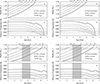 |
Fig. 16. Stellar evolution mass tracks for NY Hya A and B computed with different values of the convective mixing length parameter, αMLT = 0.75, 1.00, 1.25, 1.50, 2.04. Panelsa, c, e, g show model radii and Teffs as a function of age, respectively, for mass tracks with M = 1.160 M⊙ (NY Hya A). Decreasing αMLT leads to larger radii and cooler temperatures at a given age. Panelsb, d, f, h are the same, but computed with a model mass M = 1.168 M⊙ (NY Hya B). Solar metallicity models are shown in panelsa–d and super-solar metallicity models are shown in panelse–h. The horizontal short-dashed lines indicate the measured values from Table 11; the horizontal solid lines indicate the corresponding 1σ uncertainty. The horizontal dot-dashed lines in the Teff panels represent the Teff measured from SED fitting. The grey shaded regions indicate a model-inferred age range. |
Figures 16a–d illustrate how the model radii and Teff evolve with time for the standard case (solid line) and adjusted mixing length models (dashed lines) at solar metallicity. As is expected for inefficient convection, the stellar radius increases and the Teff decreases at a given age as the mixing length decreases. The inferred age of NY Hya is reduced to 2–4 Gyr based on radius measurements for the two components. However, an αMLT < 0.75 is required to produce agreement with the Teff (as determined from spectral synthesis) at an age consistent with stellar radii assuming a solar metallicity. To match the Teff determined from SED fitting (dot dashed line), the mixing length parameter needs to be αMLT = 1.00.
Models computed with a super-solar metallicity [Fe/H] = +0.2 require 1.00 < αMLT < 1.25, as is shown in Figs. 16e–h. One would infer an age for NY Hya of 3.1–4.5 Gyr. Increasing the metallicity further allows for main-sequence model solutions with higher values of αMLT. This is the result of higher metallicity models having naturally lower Teffs prior to αMLT adjustments. It appears that artificially lowering the convective mixing length through modifications to αMLT can produce the intended results: agreement between models and observations at a main-sequence age. Unfortunately, changing αMLT carries no immediate physical meaning. It is not possible to immediately diagnose why a reduced αMLT is required.
10.3.2. Magnetic inhibition of convection
Reducing the efficiency of convection by tuning the convective mixing length parameter (αMLT) can bring model predictions into agreement with the measured properties of NY Hya A and B. This is particularly true if the two stars have a slightly super-solar metallicity, with [Fe/H] = + 0.20. However, this approach is phenomenological in nature and does not lend physical insight as to why convection may be inefficient in these stars. One testable explanation for inefficient convection is that strong magnetic fields are inhibiting convective flows thereby suppressing convective energy transport. Magnetic inhibition of convection has been previously shown to explain differences between model predictions and observations of the properties (radii and Teffs) for the solar-type detached eclipsing binary EF Aqr (Vos et al. 2012; Feiden & Chaboyer 2012).
The hypothesis that magnetic inhibition of convection is responsible for the noted disagreements between main-sequence stellar models and the measured properties of NY Hya A and B is tested using magnetic Dartmouth stellar evolution models (Feiden & Chaboyer 2012). Individual mass tracks were computed for each NY Hya component assuming multiple initial metallicity values ([Fe/H] = [0.0, 0.2] dex) and a range of surface-averaged magnetic field strengths (⟨Bf⟩ = [0.3, 0.6, 0.9, 1.0, 1.1, 1.2] kG). The surface-averaged magnetic field is assumed to be constant throughout the model’s evolution. While not necessarily realistic, the impact of magnetic inhibition of convection on the predictions of main-sequence stellar properties at a given age were found to be insensitive to the magnetic field strength evolution (Feiden & Chaboyer 2012). Masses for the individual components were taken to be the most probable values from Table 11. Deviations from the most probable value of the order of the observed uncertainty are not large enough to affect the overall conclusions of our magnetic model analysis.
Results from our magnetic stellar model analysis for a solar and super-solar metallicity are shown in Fig. 17. We find that with magnetic models, model radii are consistent with the measured radii during the model’s main-sequence lifetime. Estimated ages are between 4 and 5 Gyr for solar metallicity models (Fig. 17a–d), and between 5 and 6 Gyr for super-solar metallictiy models (Fig. 17e–h). However, assuming an initial solar metallicity produces models with Teffs higher than the measured values by 300 K–400 K at the age where models reproduce the measured stellar radii. Adopting a super-solar initial metallicity, [Fe/H] = 0.2 dex, yields model Teffs that are about 200 K higher than the measured values. In the latter case, magnetic models agree with Teffs estimated from SED fitting (∼5800 K), but they are nevertheless discrepant with estimates from the detailed spectroscopic analysis.
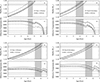 |
Fig. 17. Stellar evolution mass tracks for NY Hya A and B showing the temporal evolution of model radii and Teffs between 1 and 7 Gyr that include magnetic inhibition of convection. Mass tracks are computed with different values of the surface magnetic field strength, Bsurf = 900, 1000, 1100, 1200 G. Increasing surface magnetic field strengths leads to larger model radii and cooler Teff values at a given age. Panelsa, c, e, andg are computed with M = 1.160 M⊙ for NY Hya A, while panelsb, d, f, andh are computed with M = 1.168 M⊙ for NY Hya B. Solar metallicity models are shown in panelsa–d and super-solar metallicity models are shown in panelse–h. |
Assuming the components NY Hya A and B have Teffs more consistent with the SED fitting analysis (Teff ∼ 5800 K)33, models suggest a super-solar metallicity for the system. An initial metallicity of [Fe/H] = 0.2 dex provides a viable main-sequence solution, which after diffusion has a final metallicity of [Fe/H] = 0.1 dex. Magnetic stellar models suggest that the best-fit surfaced-averaged magnetic field is ⟨Bf⟩ = 1.0 ± 0.2 kG to provide a main-sequence solution for both stars at the same age. Given the similarities in stellar mass, the two components have approximately the same surface-averaged magnetic field strength. This restricts the age of the NY Hya system to τage = 5.3 ± 0.3 Gyr.
10.3.3. Star spots
Star spots can potentially affect stars in multiple ways depending on the timescale over which the star spots exist on the stellar surface. If star spots are transient features that appear and disappear rapidly relative to the star’s thermal timescale, spots should have a limited effect on the star’s thermal structure. Transient star spots will cause the star’s average surface temperature to appear cooler than the ambient photosphere and will cause a temporary decrease in the star’s observed luminosity. However, if star spots are not transient features, they may cause the star to restructure to maintain thermal equilibrium (e.g. Spruit 1982; Spruit & Weiss 1986; Somers et al. 2020).
We evaluate whether transient spots can produce the observed temperature disagreements between observational measurements (Table 11) and standard models (see Sect. 10.2) using a simple phenomenological model. Transient spots would leave the stellar radius unaffected and cause a decrease in bolometric luminosity due to a cooler average surface temperature. Mathematically,
where Teff is the Teff of a spotted star, Teff, 0 is the Teff of a similar unspotted star, 𝜚 is the areal surface coverage of star spots, and ϖ is the temperature ratio between the spots and ambient photosphere. Assuming that star spots on NY Hya A and B have similar characteristics to sunspots, ϖ ≈ 0.65 (Solanki 2003), each star requires an areal surface coverage of star spots 𝜚 ≈ 0.40 to produce the observed 5600 K Teff compared to solar metallicity model predictions of 6200 K. This surface coverage translates to an approximate mean surface magnetic field strength by assuming star spots are formed by equipartition strength magnetic fields (Torres et al. 2021). This yields an estimate of ⟨Bf⟩ = 760 G, which is roughly consistent with magnetic model predictions (see Sect. 10.3.2) and further supported from a semi-empirical estimate based on the observed X-ray luminosity (see Sect. 10.4).
If star spots affect a stars’ internal structure, they produce effects similar to magnetic inhibition of convection (Somers et al. 2020). We test whether long-lived star spots can explain the observed properties of the NY Hya stars using SPOTS models (Somers et al. 2020). These models assume a solar metallicity and are calculated with a fixed temperature ratio of ϖ = 0.8 between spots and the stellar photosphere. SPOTS models are computed on a fixed-mass grid, so we adopt a mass M = 1.15 M⊙ for our comparisons. Spotted models reproduce the radii of NY Hya A and B at ages between 1.75 Gyr and 4.75 Gyr, depending on the surface coverage of spots. High coverage fractions produce the observed radii at younger ages. However, only SPOTS models with a surface coverage f > 0.80 are able to reproduce the measured Teff ∼ 5600 K. In this case, the inferred age for NY Hya is τage = 2.0 ± 0.3 Gyr. By contrast, a surface coverage of f ∼ 0.55 is required to produce models with Teff ∼ 5800 K, leading to τage = 3.0 ± 0.5 Gyr.
There are a couple reasons to be sceptical of these results. First, the assumed temperature ratio ϖ = 0.8 is not necessarily representative of spot temperatures on the stars of NY Hya, which could be as low as ϖ = 0.65. Cooler spots would lead to a lower surface coverage required to reproduce the observed properties of NY Hya. Assuming luminosity is conserved during spot-driven inflation, the required surface coverages would decrease to f ∼ 0.55 and 0.40 for Teff ∼ 5600 K and 5800 K, respectively. A second reason is rooted in the assumptions built into the SPOTS models, which prescribe surface boundary conditions for stellar models based on the temperature structure for the ambient photosphere. This works well for lower surface coverages, but is a questionable assumption when spots cover over half of the stellar surface, at which point the temperature structure for the spotted surface may be more appropriate (similar to a cool star with hot spots). However, this scepticism cannot be used to rule out the possibility that star spots are responsible for difference between standard stellar models and the measured properties of NY Hya A and B.
In summary, a surface coverage of approximately 40% for each star is required for short-lived star spots to reproduce the properties of NY Hya. However, a surface coverage of 55%–80% is required if star spots are long-lived and affect stellar structure.
10.4. Semi-empirical estimate of magnetic field strength and total X-ray luminosity
We performed a consistency check on the best-fit magnetic field strength required by the non-standard stellar evolution models. An independent estimate of the surface averaged mean magnetic field strength ⟨Bf⟩ and total X-ray luminosity log LX can be obtained by following the methodology described in Torres et al. (2014).
The method is semi-empirical partially relying on theory. A power-law relationship between ⟨Bf⟩ and the Rossby number Ro = Prot/τc was given in Saar (2001) where Prot is the stellar rotation period and τc is the convection turnover time. For NY Hya, the measured rotation velocities and stellar radii for the two components are consistent with a derived stellar rotation period equal to the orbital period within uncertainties. This implies that the stars are tidally locked and rotate synchronously as noted earlier. We therefore set Prot = Porb. The convection turnover time is estimated from theory using the relationship34 in Gilliland (1986) for a given measured effective temperature.
For star A we found τc = 20.9 ± 1.2 days, and for star B τc = 20.6 ± 1.3 days, resulting in Rossby numbers of Ro = 0.229 ± 0.012 and Ro = 0.231 ± 0.012 for stars A and B, respectively. The Saar (2001) calibration relation then yields a mean magnetic field strength for star A of ⟨Bf⟩A = 327 ± 209 G and star B ⟨Bf⟩B = 323 ± 206 G confirming a near-identical mean field strength of the two components. The total uncertainty was found from MC error propagation added in quadrature to the scatter of the relationship as provided by Saar (2001).
Another estimate of the magnetic field strength may be obtained from applying a scaling relation using the core emission feature in the Ca II K line (Schrijver et al. 1989; Feiden & Chaboyer 2012). The relation was obtained from solar observations correlating magnetic field measurements with Ca II K core emissions of local photospheric active regions. The scaling relation is independent of any Doppler-shift that might occur as a result of the binary motion. We applied the relation given by Feiden & Chaboyer (2012) assuming its validity to the components of NY Hya. Rough estimates of the intensities of the core emission feature (Ic) and at the Ca II K wing (Iw; 7.4 Å to the red) were determined. We found these intensities from a normalised FEROS spectrum at phase 0.5 that allowed us to estimate the mean magnetic field strength of ⟨Bf⟩ = 959 ± 431 G of star A. This estimate is about a factor of 3 larger than the estimate obtained from Saar (2001), while in closer agreement with the 1.0 kG field strength derived from the non-standard stellar evolution model.
As a final consistency check, the mean magnetic field strength of ⟨Bf⟩ = 959 G can be transformed to an X-ray luminosity using the empirical scaling relations provided in Pevtsov et al. (2003) and Feiden & Chaboyer (2013). This provides a consistency check allowing us to compare the X-ray luminosities obtained from the mean magnetic field of each component with the total X-ray emission detected by the ROSAT satellite. Pevtsov et al. (2003) found a tightly correlated power-law relationship between the X-ray luminosity LX and the magnetic flux at the stellar surface Φ = 4πR2⟨Bf⟩ with R denoting the stellar radius. Feiden & Chaboyer (2013) expanded the Pevtsov et al. (2003) data set and provide an updated scaling relation valid over 12 orders of magnitude in both Φ and LX. For NY Hya, we found log LX = 29.7 ± 2.1 dex (with LX in erg s−1) for star A and log LX = 29.9 ± 2.0 dex for star B. These estimates are consistent with the near-identical properties of the two components. The total X-ray luminosity was found to be log LX, A + B = 30.1 ± 1.7 dex. This estimate can now be compared with the ROSAT measurement.
NY Hya has a confirmed X-ray counterpart and is included in the second ROSAT all-sky survey (2RXS ID: J092121.7-064018) source catalogue by Boller et al. (2016) listing a count rate of 0.055 ± 0.016 counts s−1 (in the 0.1–2.0 keV range) and a hardness ratio of HR1 = 0.39 ± 0.38. These measurements were obtained from a 294 s exposure (about 20 s longer than the first all-sky catalogue). The total X-ray luminosity for NY Hya is calculated from Szczygieł et al. (2008) using the Gaia (DR2) parallax and we find log LX(ROSAT) = 29.89 ± 0.18 dex.
Comparing the ROSAT measurement with the semi-empirical derived total X-ray luminosity, we find an agreement at the 0.62σ level. We conclude that the observed X-ray flux is consistent with the expected flux for a magnetically active star with ⟨Bf⟩≈1 kG. As for the case studied in Torres et al. (2014) this good agreement may be interpreted as an indication of the accuracy of the ⟨Bf⟩A, B values obtained above although their formal 1σ uncertainties are large. We conclude this section by stating that a mean magnetic field of 1 kG is plausible for each stellar component lending further credibility to non-standard magnetic stellar evolution models.
11. Discussion and conclusions
We have presented a complete analysis of astrometric, photometric, and spectroscopic data for the NY Hya eclipsing binary system. The analysis is based on the assumption that the data are correctly interpreted as being caused by the binary nature of two orbiting stars and that measurement errors follow normal statistics.
The eclipsing nature of NY Hya was discovered from HIPPARCOS photometry. The two stars were found to be identical to within the measurement errors. The classic differentiation of a primary and secondary component is therefore limited by surface activity via star spots. The combination of joint properties of two solar-twin stars and a long orbital period renders this system ideal for studying stellar evolution of solar-type stars based on the assumption that complicated tidal effects are small.
We measured the physical properties of NY Hya to high precision based on high-quality spectroscopic and light curve data. Recent astrometric measurements from Gaia provide a direct empirical, and accurate distance measurement to a high precision, enabling a reliable estimate of distance-dependent system properties, thus replacing previous semi-empirical distance estimates from photometry. We utilised the latest version of the JKTEBOP code and obtained model-independent maximum fractional uncertainties of 0.8% and 1.2% in the stellar masses and radii, respectively.
We confronted the physical properties with standard and recently developed non-standard stellar evolution models. A standard model solution that describes both stars on the main-sequence consistently for all observed properties does not appear to exist. NY Hya belongs to the group of dEB with a short orbital period. Those binaries usually fail to reproduce predictions from classic stellar evolution theories (Feiden & Chaboyer 2012; Vos et al. 2012). The resulting parameter distributions were found to be bimodal: both PMS (young age) and main-sequence turn-off (old age) solutions exist. Their validity should be viewed with scepticism due to lack of further observational evidence, in order to avoid the possibility of declaring the two components to be in a rapid phase of stellar evolution. For example, while standard models with an old age and super-solar metallicity are encouraging, they seem unlikely because i) the likelihood that both stars currently are observed just at the main-sequence turn-off (sub-giant) phase is low; ii) because the model Teffs were about 700 K cooler than the measured temperatures; iii) because observational data suggest a solar metallicity for the two components, which is in discrepancy with the super-solar metallicity as suggested by the model; and, finally, iv) standard models pointing towards a pre-main-sequence solution seem unlikely without further evidence of stellar youth. We attempted to constrain stellar age from kinematical consideration, but were not able to show NY Hya to be associated with any known nearby stellar cluster of known age. Age determination from spectral indicators requires a careful in-depth analysis. The preliminary results presented here point towards a young stellar age, but are deemed not trustworthy at the moment. Lithium absorption features were absent from the FEROS spectra.
Under the assumption that the two components are observed in their main-sequence evolutionary phase and invoking magnetic non-standard models (assuming a constant surface-averaged magnetic field throughout the simulated stellar evolution) seems to reconcile the observed tensions in Teffs. The best-fit theoretical model, however, reproduces observed properties at a super-solar metallicity and an age of approximately 5.3 Gyr. This age is consistent with the derived synchronisation and circularisation timescale. However, the required super-solar metallicity is still in conflict with the metallicity derived from our spectral synthesis analysis pointing towards solar metallicity for both components. We recall that a solar metallicity for both components is supported by Strömgren photometry, although with large uncertainties, via calibration relations.
From visual inspection of the Ca II K and H lines, we found chromospheric activity in both components. This is further substantiated with a measured X-ray excess emission by ROSAT and indicates enhanced stellar magnetic activity. The best-fit theoretical model was found at a mean magnetic field of approximately 1 kG and is found to be consistent with a semi-empirical estimate of a mean magnetic field from the detected X-ray flux.
Some tension and shortcomings are still present. First, the detailed spectroscopic analysis resulted in Teff values that are too cool compared to the mean temperature obtained from the SED analysis. The difference is significant and cannot be explained by the inferred uncertainties. Temperatures obtained from Strömgren photometry are not precise enough to provide a reliable verdict in pointing in one (5600 K) or the other direction (5800 K). The SED models also pointed towards a higher metallicity for each component, as were inferred from a direct spectral analysis. Second, the present analysis did not carry out a detailed chemical abundance study for a direct empirical estimate of metallicity for each component. Such an analysis would be advantageous to place further constraints on stellar evolution models. Although the FEROS spectra are of relatively high quality, we did experience complications when working with them in detail in an attempt to measure individual abundances. Finally, an estimate of age would be useful for the establishment of the current evolutionary stage of NY Hya. On that account age accuracy (reliability) is more important than precision to differentiate between the young and old dichotomy.
We encourage future work in an attempt to further constrain the nature (i.e. age and abundances) of this eclipsing binary. We also encourage a proper treatment of surface activity via modelling star spots directly or by removing star spot activity from the original observations.
During the final stage of analysis, we learned about the existence of additional high-quality photometric TESS and spectroscopic (ESO/HARPS) data, and will leave their analysis to a future follow-up study. The HARPS data, of likely higher quality, might be able to decide on the true Teff for each component. Furthermore, the Gaia DR2 and EDR3 point to a close (6 arcsec) companion star (Gaia DR2/EDR3 5746104876937814912), 8.5 magnitudes fainter than NY Hya, which is not visible in the Pan-STARRS images (situated within the Pan-STARRS NY Hya PSF). The contaminating flux contribution to the TESS target aperture is negligible, and is slightly fainter than the brightest of the three contaminating stars found in the Pan-STARRS images. In addition, due to the companion star being 8.5 magnitudes fainter, it was not detected in the contrast curve obtained from the TCI images, which have a sky-background contrast of 8 magnitudes fainter than NY Hya. An interesting note is that the object 5746104876937814912 seems to be a bound companion to NY Hya. The measured parallaxes agree at a 0.41σ level, consistent with the stars being at the same distance. The proper motions are different by ∼4.7 mas yr−1, which is statistically significant. This gives a projected separation of approximately 500 AU and a projected velocity difference of ∼0.5 AU yr−1, while using the masses and separation would give an expected orbital velocity of ∼0.4 AU yr−1. Thus, NY Hya seems to be part of a triple system.
https://www.eso.org/sci/facilities/lasilla/instruments/feros.html, https://www.eso.org/public/teles-instr/lasilla/mpg22/feros/, http://www.mpia.de/FEROS/about_feros.html, https://www.eso.org/public/teles-instr/lasilla/mpg22/feros/
http://www.astro.keele.ac.uk/jkt/codes/jktebop.html code, which implements the IAU 2015 Resolution B3 (Prša et al. 2016) for Solar values.
NASA/IPAC Infrared Science Archive; https://irsa.ipac.caltech.edu/applications/DUST/
Gilliland (1986) Fig. 7 was digitised and a cubic spline was determined for increased accuracy and proper error propagation.
Acknowledgments
A. Kaufer, O. Stahl, S. Tubbesing, and B. Wolf kindly observed nearly all the spectra of NY Hya during the Heidelberg/Copenhagen guaranteed time at FEROS in 1998 and 1999. This research made use of LIGHTKURVE, a PYTHON package for Kepler and TESS data analysis (Lightkurve Collaboration 2018). J. T.-R. acknowledges financial support from CONICYT/FONDECYT in terms of a 2018 Postdoctoral research grant, project number: 3180071. T.C.H. would like to acknowledge fruitful conversations with the following individuals: Arne Henden, Patrick Lenz, Eric Mamajek, Guillermo (Willie) Torres and Ignasi Ribas who also kindly provided details of CORAVEL data. This research has received funding from the Europlanet 2024 Research Infrastructure (RI) programme. The Europlanet 2024 RI provides free access to the world’s largest collection of planetary simulation and analysis facilities, data services and tools, a ground-based observational network and programme of community support activities. Europlanet 2024 RI has received funding from the European Union’s Horizon 2020 research and innovation programme under grant agreement No. 871149. This research has made use of the SVO Filter Profile Service (http://svo2.cab.inta-csic.es/theory/fps/) supported from the Spanish MINECO through grant AYA2017-84089. J. V. Clausen participated fully in the data collection and analysis up to the time of his death, but bears no responsibility for the final text of this paper. B. E. Helt participated fully in the data collection and analysis up to the time of her death in 2023, but bears no responsibility for the final text of this paper. E. H. Olsen participated fully in the data collection and analysis (especially data described in Sect. 2.1) up to the time of his death on March 1, 2024, but bears no responsibility for the final text of this paper. N.P.’s work was supported by Fundação para a Ciência e a Tecnologia (FCT) through the research grants UIDB/04434/2020 and UIDP/04434/2020. U.G.J. acknowledges funding from the Novo Nordisk Foundation Interdisciplinary Synergy Programme grant no. NNF19OC0057374 and from the European Union H2020-MSCA-ITN-2019 under Grant no. 860470 (CHAMELEON). J.V. acknowledges support from the Grant Agency of the Czech Republic (GAČR 22-34467S). The Astronomical Institute Ondřejov is supported by the project RVO:67985815. J.C.M. acknowledges financial support by Spanish grants PID2021-125627OB-C31 funded by MCIU/AEI/10.13039/501100011033 and by “ERDF A way of making Europe”, PGC2018-098153-B-C33 funded by MCIU/AEI, by the programme Unidad de Excelencia María de Maeztu CEX2020-001058-M, and by the Generalitat de Catalunya/CERCA programme. P.L.P. was partly funded by Programa de Iniciación en Investigación-Universidad de Antofagasta. INI-17-03
References
- Allard, F., Hauschildt, P. H., Miller, S., & Tennyson, J. 1994, ApJ, 426, L39 [NASA ADS] [CrossRef] [Google Scholar]
- Allard, F., Homeier, D., & Freytag, B. 2012, Philos. Trans. Roy. Soc. London Ser. A, 370, 2765 [Google Scholar]
- Alonso, A., Arribas, S., & Martinez-Roger, C. 1996, A&A, 313, 873 [NASA ADS] [Google Scholar]
- Andersen, J. 1991, A&A Rev., 3, 91 [Google Scholar]
- Andersen, J., Clausen, J. V., & Nordstrom, B. 1990, A&A, 228, 365 [NASA ADS] [Google Scholar]
- Andrae, R. 2010, ArXiv e-prints [arXiv:1009.2755] [Google Scholar]
- Árnadóttir, A. S., Feltzing, S., & Lundström, I. 2010, A&A, 521, A40 [NASA ADS] [CrossRef] [EDP Sciences] [Google Scholar]
- Asplund, M., Grevesse, N., Sauval, A. J., & Scott, P. 2009, ARA&A, 47, 481 [NASA ADS] [CrossRef] [Google Scholar]
- Aumer, M., & Binney, J. J. 2009, MNRAS, 397, 1286 [NASA ADS] [CrossRef] [Google Scholar]
- Baraffe, I., Homeier, D., Allard, F., & Chabrier, G. 2015, A&A, 577, A42 [NASA ADS] [CrossRef] [EDP Sciences] [Google Scholar]
- Bayo, A., Rodrigo, C., Barrado Y Navascués, D., et al. 2008, A&A, 492, 277 [NASA ADS] [CrossRef] [EDP Sciences] [Google Scholar]
- Bensby, T., Feltzing, S., & Lundström, I. 2003, A&A, 410, 527 [CrossRef] [EDP Sciences] [Google Scholar]
- Bensby, T., Feltzing, S., & Oey, M. S. 2014, A&A, 562, A71 [NASA ADS] [CrossRef] [EDP Sciences] [Google Scholar]
- Bessell, M. S., Castelli, F., & Plez, B. 1998, A&A, 333, 231 [NASA ADS] [Google Scholar]
- Bianchi, L., Herald, J., Efremova, B., et al. 2011, Ap&SS, 335, 161 [Google Scholar]
- Blanco-Cuaresma, S. 2019, MNRAS, 486, 2075 [Google Scholar]
- Blanco-Cuaresma, S., Soubiran, C., Heiter, U., & Jofré, P. 2014, A&A, 569, A111 [CrossRef] [EDP Sciences] [Google Scholar]
- Boller, T., Freyberg, M. J., Trümper, J., et al. 2016, A&A, 588, A103 [NASA ADS] [CrossRef] [EDP Sciences] [Google Scholar]
- Caffau, E., Maiorca, E., Bonifacio, P., et al. 2009, A&A, 498, 877 [NASA ADS] [CrossRef] [EDP Sciences] [Google Scholar]
- Cannon, A. J., & Pickering, E. C. 1993, VizieR Online Data Catalog: III/135A [Google Scholar]
- Capitanio, L., Lallement, R., Vergely, J. L., Elyajouri, M., & Monreal-Ibero, A. 2017, A&A, 606, A65 [NASA ADS] [CrossRef] [EDP Sciences] [Google Scholar]
- Casagrande, L., Schönrich, R., Asplund, M., et al. 2011, A&A, 530, A138 [NASA ADS] [CrossRef] [EDP Sciences] [Google Scholar]
- Cassisi, S. 2005, ArXiv e-prints [arXiv:astro-ph/0506161] [Google Scholar]
- Castelli, F., & Kurucz, R. L. 2003, in Modelling of Stellar Atmospheres, eds. N. Piskunov, W. W. Weiss, & D. F. Gray, 210, A20 [Google Scholar]
- Chabrier, G., Gallardo, J., & Baraffe, I. 2007, A&A, 472, L17 [CrossRef] [EDP Sciences] [Google Scholar]
- Chambers, K. C., Magnier, E. A., Metcalfe, N., et al. 2016, ArXiv e-prints [arXiv:1612.05560] [Google Scholar]
- Clausen, J. V., Helt, B. E., & Olsen, E. H. 2001, A&A, 374, 980 [NASA ADS] [CrossRef] [EDP Sciences] [Google Scholar]
- Clausen, J. V., Torres, G., Bruntt, H., et al. 2008, A&A, 487, 1095 [NASA ADS] [CrossRef] [EDP Sciences] [Google Scholar]
- Clausen, J. V., Bruntt, H., Claret, A., et al. 2009, A&A, 502, 253 [NASA ADS] [CrossRef] [EDP Sciences] [Google Scholar]
- Coelho, P. R. T. 2014, MNRAS, 440, 1027 [Google Scholar]
- Crawford, D. L. 1975, PASP, 87, 481 [NASA ADS] [CrossRef] [Google Scholar]
- Crawford, D. L., & Barnes, J. V. 1970, AJ, 75, 978 [NASA ADS] [CrossRef] [Google Scholar]
- Crawford, D. L., & Mandwewala, N. 1976, PASP, 88, 917 [CrossRef] [Google Scholar]
- Dotson, J., Barentsen, G., Hedges, C. L., et al. 2019, Am. Astron. Soc. Meeting Abstracts, 233, 445.01 [NASA ADS] [Google Scholar]
- Dotter, A., Chaboyer, B., Jevremović, D., et al. 2008, ApJS, 178, 89 [Google Scholar]
- Eastman, J., Siverd, R., & Gaudi, B. S. 2010, PASP, 122, 935 [Google Scholar]
- ESA 1997, in The HIPPARCOS and TYCHO catalogues. Astrometric and photometric star catalogues derived from the ESA HIPPARCOS Space Astrometry Mission, ESA Spec. Pub., 1200 [Google Scholar]
- Etzel, P. B. 1975, Master’s Thesis, San Diego State University, USA [Google Scholar]
- Etzel, P. B. 1981, in Photometric and Spectroscopic Binary Systems, eds. E. B. Carling, & Z. Kopal, NATO ASI Ser. C, 69, 111 [NASA ADS] [CrossRef] [Google Scholar]
- Evans, D. F., Southworth, J., Maxted, P. F. L., et al. 2016, A&A, 589, A58 [NASA ADS] [CrossRef] [EDP Sciences] [Google Scholar]
- Feiden, G. A. 2016, A&A, 593, A99 [NASA ADS] [CrossRef] [EDP Sciences] [Google Scholar]
- Feiden, G. A., & Chaboyer, B. 2012, ApJ, 761, 30 [NASA ADS] [CrossRef] [Google Scholar]
- Feiden, G. A., & Chaboyer, B. 2013, ApJ, 779, 183 [Google Scholar]
- Feiden, G. A., Skidmore, K., & Jao, W.-C. 2021, ApJ, 907, 53 [NASA ADS] [CrossRef] [Google Scholar]
- Fitzpatrick, E. L. 1999, PASP, 111, 63 [Google Scholar]
- Flewelling, H. 2016, Am. Astron. Soc. Meeting Abstracts, 227, 144.25 [NASA ADS] [Google Scholar]
- Flewelling, H. A., Magnier, E. A., Chambers, K. C., et al. 2020, ApJS, 251, 7 [NASA ADS] [CrossRef] [Google Scholar]
- Florentin-Nielsen, R., Nörregaard, P., & Olsen, E. H. 1987, The ESO Messenger, 50, 45 [NASA ADS] [Google Scholar]
- Foreman-Mackey, D. 2016, J. Open Source Software, 1, 24 [NASA ADS] [CrossRef] [Google Scholar]
- Foreman-Mackey, D., Hogg, D. W., Lang, D., & Goodman, J. 2013, PASP, 125, 306 [Google Scholar]
- Gagné, J., Mamajek, E. E., Malo, L., et al. 2018, ApJ, 856, 23 [Google Scholar]
- Gaia Collaboration (Brown, A. G. A., et al.) 2018, A&A, 616, A1 [NASA ADS] [CrossRef] [EDP Sciences] [Google Scholar]
- Gaia Collaboration (Brown, A. G. A., et al.) 2021, A&A, 649, A1 [NASA ADS] [CrossRef] [EDP Sciences] [Google Scholar]
- Gáspár, A., Rieke, G. H., & Ballering, N. 2016, ApJ, 826, 171 [Google Scholar]
- Gilliland, R. L. 1986, ApJ, 300, 339 [NASA ADS] [CrossRef] [Google Scholar]
- Girardi, L., Bertelli, G., Bressan, A., et al. 2002, A&A, 391, 195 [NASA ADS] [CrossRef] [EDP Sciences] [Google Scholar]
- Green, G. M., Schlafly, E. F., Finkbeiner, D. P., et al. 2014, ApJ, 783, 114 [NASA ADS] [CrossRef] [Google Scholar]
- Green, G. M., Schlafly, E. F., Finkbeiner, D., et al. 2018, MNRAS, 478, 651 [Google Scholar]
- Grevesse, N., & Noels, A. 1993, in Origin and Evolution of the Elements, eds. N. Prantzos, E. Vangioni-Flam, & M. Casse, 15 [Google Scholar]
- Grevesse, N., & Sauval, A. J. 1998, Space Sci. Rev., 85, 161 [Google Scholar]
- Grevesse, N., Asplund, M., & Sauval, A. J. 2007, Space Sci. Rev., 130, 105 [Google Scholar]
- Hauschildt, P. H., Allard, F., & Baron, E. 1999, ApJ, 512, 377 [Google Scholar]
- Henden, A. A., Levine, S., Terrell, D., & Welch, D. L. 2015, Am. Astron. Soc. Meeting Abstracts, 225, 336.16 [NASA ADS] [Google Scholar]
- Høg, E., Fabricius, C., Makarov, V. V., et al. 2000, A&A, 355, L27 [Google Scholar]
- Holmberg, J., Nordström, B., & Andersen, J. 2007, A&A, 475, 519 [CrossRef] [EDP Sciences] [Google Scholar]
- Holmberg, J., Nordström, B., & Andersen, J. 2009, A&A, 501, 941 [NASA ADS] [CrossRef] [EDP Sciences] [Google Scholar]
- Houk, N., & Swift, C. 1999, Michigan Catalogue of Two-dimensional Spectral Types for the HD Stars; vol. 5 (Ann Arbor, Michigan, USA: Department of Astronomy, University of Michigan) [Google Scholar]
- Hughes, I. G., & Hase, T. P. A. 2010, Measurements and their Uncertainties - a Practical Guide to Modern Error Analysis (Oxford University Press) [Google Scholar]
- Hut, P. 1981, A&A, 99, 126 [NASA ADS] [Google Scholar]
- Iglesias-Marzoa, R., López-Morales, M., & Jesús Arévalo Morales, M. 2015, PASP, 127, 567 [NASA ADS] [CrossRef] [Google Scholar]
- Ilijic, S., Hensberge, H., Pavlovski, K., & Freyhammer, L. M. 2004, in Spectroscopically and Spatially Resolving the Components of the Close Binary Stars, eds. R. W. Hilditch, H. Hensberge, & K. Pavlovski, ASP Conf. Ser., 318, 111 [Google Scholar]
- Isaacson, H., & Fischer, D. 2010, ApJ, 725, 875 [Google Scholar]
- Jenkins, J. M., Twicken, J. D., McCauliff, S., et al. 2016, in Software and Cyberinfrastructure for Astronomy IV, eds. G. Chiozzi, & J. C. Guzman, SPIE Conf. Ser., 9913, 99133E [Google Scholar]
- Kallrath, J., & Milone, E. F. 2009, Eclipsing Binary Stars: Modeling and Analysis (New York, USA: Springer-Verlag) [CrossRef] [Google Scholar]
- Karataş, Y., & Schuster, W. J. 2010, New A, 15, 444 [CrossRef] [Google Scholar]
- Kaufer, A., Stahl, O., Tubbesing, S., et al. 1999, The Messenger, 95, 8 [Google Scholar]
- Kazarovets, E. V., Samus, N. N., Durlevich, O. V., et al. 1999, Inf. Bull. Var. Stars, 4659, 1 [Google Scholar]
- Kervella, P., Thévenin, F., Di Folco, E., & Ségransan, D. 2004, A&A, 426, 297 [NASA ADS] [CrossRef] [EDP Sciences] [Google Scholar]
- Kochukhov, O. P. 2007, in Physics of Magnetic Stars, eds. I. I. Romanyuk, D. O. Kudryavtsev, O. M. Neizvestnaya, & V. M. Shapoval, 109 [Google Scholar]
- Kochukhov, O. 2018, Astrophysics Source Code Library [record ascl:1805.015] [Google Scholar]
- Kreiner, J. M. 2004, Acta Astron., 54, 207 [NASA ADS] [Google Scholar]
- Kurucz, R. L. 1993, SYNTHE Spectrum Synthesis Programs and Line Data (Cambridge, MA, USA: Smithsonian Astrophysical Observatory) [Google Scholar]
- Kwee, K. K., & van Woerden, H. 1956, Bull. Astron. Inst. Netherlands, 12, 327 [Google Scholar]
- Lallement, R., Vergely, J. L., Valette, B., et al. 2014, A&A, 561, A91 [NASA ADS] [CrossRef] [EDP Sciences] [Google Scholar]
- Lenz, P. 2005, PhD Thesis, University of Vienna, Austria [Google Scholar]
- Lenz, P., & Breger, M. 2005, Commun. Asteroseismol., 146, 53 [Google Scholar]
- Li, L.-S. 2018, JKAS, 51, 1 [Google Scholar]
- Lightkurve Collaboration (Cardoso, J. V. d. M., et al.) 2018, Astrophysics Source Code Library [record ascl:1812.013] [Google Scholar]
- Lockwood, G. W., Skiff, B. A., & Radick, R. R. 1997, ApJ, 485, 789 [NASA ADS] [CrossRef] [Google Scholar]
- Lucy, L. B., & Sweeney, M. A. 1971, AJ, 76, 544 [NASA ADS] [CrossRef] [Google Scholar]
- Mamajek, E. 2014, Figshare https://doi.org/10.6084/m9.figshare.949735.v1 [Google Scholar]
- Mamajek, E. E., & Hillenbrand, L. A. 2008, ApJ, 687, 1264 [Google Scholar]
- Mann, A. W., Feiden, G. A., Gaidos, E., Boyajian, T., & von Braun, K. 2015, ApJ, 804, 64 [Google Scholar]
- Maxted, P. F. L., Hutcheon, R. J., Torres, G., et al. 2015, A&A, 578, A25 [NASA ADS] [CrossRef] [EDP Sciences] [Google Scholar]
- Mazeh, T., & Zucker, S. 1994, Ap&SS, 212, 349 [NASA ADS] [CrossRef] [Google Scholar]
- McDonald, I., Zijlstra, A. A., & Boyer, M. L. 2012, MNRAS, 427, 343 [Google Scholar]
- Nelson, B., & Davis, W. D. 1972, ApJ, 174, 617 [NASA ADS] [CrossRef] [Google Scholar]
- Nordström, B., Mayor, M., Andersen, J., et al. 2004, A&A, 418, 989 [Google Scholar]
- North, P., & Zahn, J. P. 2004, New A Rev., 48, 741 [NASA ADS] [CrossRef] [Google Scholar]
- Olsen, E. H. 1984, A&AS, 57, 443 [NASA ADS] [Google Scholar]
- Olsen, E. H. 1994, A&AS, 104, 429 [NASA ADS] [Google Scholar]
- Pace, G. 2013, A&A, 551, L8 [NASA ADS] [CrossRef] [EDP Sciences] [Google Scholar]
- Paturel, G., Petit, C., Rousseau, J., & Vauglin, I. 2003, A&A, 405, 1 [NASA ADS] [CrossRef] [EDP Sciences] [Google Scholar]
- Paunzen, E. 2015, A&A, 580, A23 [NASA ADS] [CrossRef] [EDP Sciences] [Google Scholar]
- Pavlovski, K., Tamajo, E., Koubský, P., et al. 2009, MNRAS, 400, 791 [NASA ADS] [CrossRef] [Google Scholar]
- Perry, C. L., Johnston, L., & Crawford, D. L. 1982, AJ, 87, 1751 [NASA ADS] [CrossRef] [Google Scholar]
- Petrie, R. M. 1939, Pub. Dominion Astrophys. Obs. Victoria, 7, 205 [NASA ADS] [Google Scholar]
- Pevtsov, A. A., Fisher, G. H., Acton, L. W., et al. 2003, ApJ, 598, 1387 [Google Scholar]
- Piskunov, N. E. 1992, Physics and Evolution of Stars, Stellar Magnetism, 92 [Google Scholar]
- Piskunov, N. E., Kupka, F., Ryabchikova, T. A., Weiss, W. W., & Jeffery, C. S. 1995, A&AS, 112, 525 [Google Scholar]
- Pojmanski, G. 1997, Acta Astron., 47, 467 [Google Scholar]
- Popper, D. M. 1997, AJ, 114, 1195 [Google Scholar]
- Popper, D. M., & Etzel, P. B. 1981, AJ, 86, 102 [NASA ADS] [CrossRef] [Google Scholar]
- Press, W. H., Teukolsky, S. A., Vetterling, W. T., & Flannery, B. P. 1992, Numerical Recipes in FORTRAN. The Art of Scientific Computing (Cambridge University Press) [Google Scholar]
- Prugniel, Ph., Soubiran, C., Koleva, M., & Le Borgne, D. 2007, ArXiv e-prints [arXiv:astro-ph/0703658] [Google Scholar]
- Prša, A., Harmanec, P., Torres, G., et al. 2016, AJ, 152, 41 [Google Scholar]
- Reddy, B. E., Lambert, D. L., & Allende Prieto, C. 2006, MNRAS, 367, 1329 [Google Scholar]
- Reegen, P. 2007, A&A, 467, 1353 [NASA ADS] [CrossRef] [EDP Sciences] [Google Scholar]
- Reis, W., Corradi, W., de Avillez, M. A., & Santos, F. P. 2011, ApJ, 734, 8 [NASA ADS] [CrossRef] [Google Scholar]
- Ribas, I. 1999, PhD Thesis, University of Barcelona, Spain [Google Scholar]
- Ribas, I. 2003, A&A, 398, 239 [NASA ADS] [CrossRef] [EDP Sciences] [Google Scholar]
- Ricker, G. R., Latham, D. W., Vanderspek, R. K., et al. 2009, Am. Astron. Soc. Meeting Abstracts, 213, 403.01 [NASA ADS] [Google Scholar]
- Ricker, G. R., Winn, J. N., Vanderspek, R., et al. 2014, in Space Telescopes and Instrumentation 2014: Optical, Infrared, and Millimeter Wave, eds. J. Oschmann, M. Jacobus, M. Clampin, G. G. Fazio, & H. A. MacEwen, SPIE Conf. Ser., 9143, 914320 [Google Scholar]
- Ricker, G. R., Winn, J. N., Vanderspek, R., et al. 2015, J. Astron. Telesc., Instrum. Syst., 1, 014003 [Google Scholar]
- Robinson, S. E., Ammons, S. M., Kretke, K. A., et al. 2007, ApJS, 169, 430 [NASA ADS] [CrossRef] [Google Scholar]
- Rodrigo, C., & Solano, E. 2013, in Highlights of Spanish Astrophysics VII, eds. J. C. Guirado, L. M. Lara, V. Quilis, & J. Gorgas, 953 [Google Scholar]
- Rodrigo, C., & Solano, E. 2020, Contributions to the XIV.0 Scientific Meeting (virtual) of the Spanish Astronomical Society, 182 [Google Scholar]
- Rodrigo, C., Solano, E., & Bayo, A. 2012, SVO Filter Profile Service Version 1.0, IVOA Working Draft [Google Scholar]
- Rucinski, S. 1999, Turk. J. Phys., 23, 271 [Google Scholar]
- Saar, S. H. 2001, in 11th Cambridge Workshop on Cool Stars, Stellar Systems and the Sun, eds. R. J. Garcia Lopez, R. Rebolo, & M. R. Zapaterio Osorio, ASP Conf. Ser., 223, 292 [Google Scholar]
- Schlafly, E. F., & Finkbeiner, D. P. 2011, ApJ, 737, 103 [Google Scholar]
- Schlegel, D. J., Finkbeiner, D. P., & Davis, M. 1998, ApJ, 500, 525 [Google Scholar]
- Schönrich, R., Binney, J., & Dehnen, W. 2010, MNRAS, 403, 1829 [CrossRef] [Google Scholar]
- Schrijver, C. J., Cote, J., Zwaan, C., & Saar, S. H. 1989, ApJ, 337, 964 [NASA ADS] [CrossRef] [Google Scholar]
- Schultz, G. V., & Wiemer, W. 1975, A&A, 43, 133 [NASA ADS] [Google Scholar]
- Schuster, W. J., & Nissen, P. E. 1989, A&A, 221, 65 [NASA ADS] [Google Scholar]
- Skottfelt, J., Bramich, D. M., Hundertmark, M., et al. 2015, A&A, 574, A54 [NASA ADS] [CrossRef] [EDP Sciences] [Google Scholar]
- Skrutskie, M. F., Cutri, R. M., Stiening, R., et al. 2006, AJ, 131, 1163 [NASA ADS] [CrossRef] [Google Scholar]
- Solanki, S. K. 2003, A&A Rev., 11, 153 [NASA ADS] [CrossRef] [Google Scholar]
- Somers, G., Cao, L., & Pinsonneault, M. H. 2020, ApJ, 891, 29 [Google Scholar]
- Soubiran, C., Bienaymé, O., & Siebert, A. 2003, A&A, 398, 141 [NASA ADS] [CrossRef] [EDP Sciences] [Google Scholar]
- Southworth, J. 2011, MNRAS, 417, 2166 [Google Scholar]
- Southworth, J. 2013, A&A, 557, A119 [NASA ADS] [CrossRef] [EDP Sciences] [Google Scholar]
- Southworth, J. 2015, in Living Together: Planets, Host Stars and Binaries, eds. S. M. Rucinski, G. Torres, & M. Zejda, ASP Conf. Ser., 496, 164 [Google Scholar]
- Southworth, J. 2022, The Observatory, 142, 267 [NASA ADS] [Google Scholar]
- Southworth, J., & Clausen, J. V. 2007, A&A, 461, 1077 [NASA ADS] [CrossRef] [EDP Sciences] [Google Scholar]
- Southworth, J., Maxted, P. F. L., & Smalley, B. 2004a, MNRAS, 349, 547 [CrossRef] [Google Scholar]
- Southworth, J., Maxted, P. F. L., & Smalley, B. 2004b, MNRAS, 351, 1277 [NASA ADS] [CrossRef] [Google Scholar]
- Southworth, J., Maxted, P. F. L., & Smalley, B. 2005a, A&A, 429, 645 [NASA ADS] [CrossRef] [EDP Sciences] [Google Scholar]
- Southworth, J., Smalley, B., Maxted, P. F. L., Claret, A., & Etzel, P. B. 2005b, MNRAS, 363, 529 [NASA ADS] [CrossRef] [Google Scholar]
- Southworth, J., Bruntt, H., & Buzasi, D. L. 2007, A&A, 467, 1215 [NASA ADS] [CrossRef] [EDP Sciences] [Google Scholar]
- Spruit, H. C. 1982, A&A, 108, 348 [NASA ADS] [Google Scholar]
- Spruit, H. C., & Weiss, A. 1986, A&A, 166, 167 [NASA ADS] [Google Scholar]
- Stassun, K. G., & Torres, G. 2021, ApJ, 907, L33 [NASA ADS] [CrossRef] [Google Scholar]
- Stassun, K. G., Oelkers, R. J., Pepper, J., et al. 2018, AJ, 156, 183 [NASA ADS] [CrossRef] [Google Scholar]
- Stassun, K. G., Oelkers, R. J., Paegert, M., et al. 2019, AJ, 158, 138 [Google Scholar]
- Swayne, M. I., Maxted, P. F. L., Hodžić, V. K., & Triaud, A. H. M. J. 2020, MNRAS, 498, L15 [NASA ADS] [CrossRef] [Google Scholar]
- Szczygieł, D. M., Socrates, A., Paczyński, B., Pojmański, G., & Pilecki, B. 2008, Acta Astron., 58, 405 [NASA ADS] [Google Scholar]
- Tonry, J., & Davis, M. 1979, AJ, 84, 1511 [Google Scholar]
- Torres, G., & Ribas, I. 2002, ApJ, 567, 1140 [Google Scholar]
- Torres, G., Stefanik, R. P., Andersen, J., et al. 1997, AJ, 114, 2764 [NASA ADS] [CrossRef] [Google Scholar]
- Torres, G., Lacy, C. H. S., Claret, A., & Sabby, J. A. 2000, AJ, 120, 3226 [Google Scholar]
- Torres, G., Andersen, J., & Giménez, A. 2010, A&A Rev., 18, 67 [Google Scholar]
- Torres, G., Sandberg Lacy, C. H., Pavlovski, K., et al. 2014, ApJ, 797, 31 [Google Scholar]
- Torres, G., Feiden, G. A., Vanderburg, A., & Curtis, J. L. 2021, Galaxies, 10, 3 [NASA ADS] [CrossRef] [Google Scholar]
- Tsantaki, M., Sousa, S. G., Adibekyan, V. Z., et al. 2013, A&A, 555, A150 [NASA ADS] [CrossRef] [EDP Sciences] [Google Scholar]
- Turner, J. D., Pearson, K. A., Biddle, L. I., et al. 2016, MNRAS, 459, 789 [NASA ADS] [CrossRef] [Google Scholar]
- Valenti, J. A., & Fischer, D. A. 2005, ApJS, 159, 141 [Google Scholar]
- Valenti, J. A., & Piskunov, N. 1996, A&AS, 118, 595 [NASA ADS] [CrossRef] [EDP Sciences] [Google Scholar]
- van Leeuwen, F. 2007, A&A, 474, 653 [CrossRef] [EDP Sciences] [Google Scholar]
- Vos, J., Clausen, J. V., Jørgensen, U. G., et al. 2012, A&A, 540, A64 [NASA ADS] [CrossRef] [EDP Sciences] [Google Scholar]
- Wilson, R. E. 1979, ApJ, 234, 1054 [Google Scholar]
- Winn, J. N. 2010, Exoplanets, ed. S. Seager (Tucson, AZ, USA: University of Arizona Press), 55 [Google Scholar]
- Wright, E. L., Eisenhardt, P. R. M., Mainzer, A. K., et al. 2010, AJ, 140, 1868 [Google Scholar]
- Zacharias, N., Finch, C., Subasavage, J., et al. 2015, AJ, 150, 101 [Google Scholar]
- Zahn, J. P. 1977, A&A, 500, 121 [NASA ADS] [Google Scholar]
- Zahn, J. P. 1989, A&A, 220, 112 [Google Scholar]
Appendix A: Spectroscopic observations of NY Hya
Log notes on spectroscopic (FEROS) observations of NY Hya.
Appendix B: RV measurements from TODCOR
RV measurements from TODCOR.
Appendix C: Corner plots of parameter uncertainty covariances and parent distribution
 |
Fig. C.1. Parameter uncertainty covariances and parameter parent distributions of light curve parameter based on TESS data analysis. We show the results from JKTEBOP task8 (MC, 5000 samples). We plot 16%, 50% and 84% quantiles for each histogram and 1σ, 2σ and 3σ confidence regions as contours. A strong negative correlation is found between the inclination (i) and sum of fractional radii (rA + rB). We omit the explicit calculation of the correlation coefficients. The orbital period (P) and reference epoch (T0) have been omitted since their covariance has been minimized by construction already. We do not show the results from PB-RP due to a low number of samples resulting in technical complications in rendering correct confidence limits. However, parameter covariances between MC and PB-RP are similar. The plots were generated with CORNER (Foreman-Mackey 2016). |
All Tables
Photometric data for NY Hya and the comparison stars HD 82074, HD 80446, and HD 80633.
Times of primary (P) and secondary (S) minima of NY Hya from SAT data only (combined 97/98 and 98/99 season).
Best-fit parameters to the TESS and FEROS data for fixed values of k as obtained from SAT y band data with proper error propagation.
Extinction-corrected Johnson V magnitude (from extinction law) and de-reddened Strömgren colour indices for NY Hya and (constant) check stars.
Physical properties of the two components in NY Hya as derived from TESS photometry and FEROS spectral data.
All Figures
|
Fig. 1. Photometric images of NY Hya from two different instruments. Top panel: camera 1 and CCD 1 target pixel file image of the first TESS cadence for NY Hya. The TESS target aperture mask used to generate the SAP light curve is highlighted in red. Bottom panel: SAP aperture superimposed on a Pan-STARRS image. North is up and east is left. Each box is 21 × 21 arcsec in size. Three faint companions are positioned at around 22 arcsec from NY Hya. |
| In the text | |
|
Fig. 2. Extracted TESS SAP light curve of NY Hya from Sector 8 with a sampling of 2 min. The first eclipse is a primary eclipse. Five primary and three secondary eclipses were observed. Some out-of-eclipse variation is clearly detected. The increase in flux at BJD 2 458 536 changes depending on the parameters used in the LIGHTKURVE detrending process. We therefore believe that this is systematic noise. |
| In the text | |
|
Fig. 3. 5σ detection contrast-curves (Δmag) from the TCI images using the top 20% stacked frames. Inset images are 10 × 10 arcsec. The full width at half maximum (seeing) was measured to be 0.97 arcsec in v and 0.85 arcsec in z. |
| In the text | |
|
Fig. 4. Strong parameter correlation (Torres et al. 2000) between light ratio lB/lA and radius ratio for TESS and SAT data. The horizontal lines show the spectroscopic light ratio for the TESS passband and its uncertainty. |
| In the text | |
|
Fig. 5. Strömgren (SAT) uvby light curves of NY Hya. We show data from the 97/98 and the 98/99 season. The solid line shows the best-fit model obtained from JKTEBOP. The residuals are shown below each model fit. |
| In the text | |
|
Fig. 6. Result of simultaneous JKTEBOP fitting of NY Hya. Observational data are shown in red and best-fit models as solid lines. No error bars are plotted. Left column: TESS light curve (top) and FEROS RV curves (bottom). Right column: details of the primary (top) and secondary (bottom) eclipse clearly showing the presence of time-correlated red noise in the residuals. |
| In the text | |
|
Fig. 7. Durbin-Watson (lag) plots for the three different data sets: TESS, RVs of star A, and RVs of star B. A 𝒟 = 2.0 indicates no auto-correlation with data randomly distributed following a standard normal distribution. For the TESS data and the RV data of star B (based on two outliers) we see a positive auto-correlation, while for the RVs of star A we see a negative auto-correlation. |
| In the text | |
|
Fig. 8. Model and disentangled observed FEROS spectrum in the 4090–4140 Å region. Top panel: disentangled spectrum of star A (plus symbols) and its best model. Bottom panel: same content, but for star B. |
| In the text | |
|
Fig. 9. Same as Fig. 8, but for the 5202–5214 Å region for star A (top panel) and star B (bottom panel). |
| In the text | |
|
Fig. 10. VOSA SED model fits (corrected for extinction) for various data sets of flux measurements for NY Hya. The horizontal lines in the residual plots mark ±3σ deviation from the model. Panel A: WISE and 2MASS flux measurements |
| In the text | |
|
Fig. 11. Results of the period analysis for the SAT 97/98 y-band data set. Panel A: 404 y out-of-eclipse photometry showing magnitude vs. time where the primary and secondary eclipses have been removed. The horizontal line is the mean flux out of the eclipses as determined by PERIOD04 and was subtracted prior to the computation of the Fourier spectrum. Panel B: power spectrum and 1, 2, and 3σ noise levels. A frequency at f1 = 0.2138 c/d is detected corresponding to a period of 4.68 days. Frequencies near 1 c/d are likely daily/nightly alias frequencies. Panel C: power spectrum of the spectral (data gap structure) window. Panel D: power spectrum after removing the f1 frequency component with the highest power. Panels B and D have the same scale along the y-axis. |
| In the text | |
|
Fig. 12. Normalised TESS baseline flux (with eclipses) phases folded with the orbital period of NY Hya. The different colours encode successive times in the order black, red, green, blue, pink and yellow. |
| In the text | |
|
Fig. 13. Wavelength region around the Ca II K and H lines (3933.66 Å and 3968.47 Å) at different orbital phases. Core emission lines are visible for both components demonstrating chromospheric activity. The outermost vertical lines mark the location of the V and R continuum bands at 3901.07 Å and 4001.70 Å. |
| In the text | |
|
Fig. 14. Mass-radius (top panel) and mass-Teff (bottom panel) diagrams showing the components of NY Hya (solid points) against three standard Dartmouth stellar evolution models. The age-metallicity combinations of the isochrones are ([Fe/H], τage) = (+0.0, 4.4 Gyr; solid line), (+0.2, 5.7 Gyr; dashed line), and (+0.4, 7.3 Gyr; dash-dotted line). |
| In the text | |
|
Fig. 15. Hertzsprung-Russell diagram showing the two components of NY Hya (solid points) against three standard Dartmouth stellar evolution model isochrones (solid lines) and a single stellar evolution model mass track (dotted line). Isochrones are shown with the same line style to provide contrast with the individual mass track. From left to right (warmer to cooler), the isochrones are ([Fe/H], τage) = (+0.0, 4.4 Gyr), (+0.2, 5.7 Gyr), and (+0.4, 7.3 Gyr). The stellar evolution mass track is showing an M = 1.160 M⊙ model with [Fe/H] = +0.4. |
| In the text | |
|
Fig. 16. Stellar evolution mass tracks for NY Hya A and B computed with different values of the convective mixing length parameter, αMLT = 0.75, 1.00, 1.25, 1.50, 2.04. Panelsa, c, e, g show model radii and Teffs as a function of age, respectively, for mass tracks with M = 1.160 M⊙ (NY Hya A). Decreasing αMLT leads to larger radii and cooler temperatures at a given age. Panelsb, d, f, h are the same, but computed with a model mass M = 1.168 M⊙ (NY Hya B). Solar metallicity models are shown in panelsa–d and super-solar metallicity models are shown in panelse–h. The horizontal short-dashed lines indicate the measured values from Table 11; the horizontal solid lines indicate the corresponding 1σ uncertainty. The horizontal dot-dashed lines in the Teff panels represent the Teff measured from SED fitting. The grey shaded regions indicate a model-inferred age range. |
| In the text | |
|
Fig. 17. Stellar evolution mass tracks for NY Hya A and B showing the temporal evolution of model radii and Teffs between 1 and 7 Gyr that include magnetic inhibition of convection. Mass tracks are computed with different values of the surface magnetic field strength, Bsurf = 900, 1000, 1100, 1200 G. Increasing surface magnetic field strengths leads to larger model radii and cooler Teff values at a given age. Panelsa, c, e, andg are computed with M = 1.160 M⊙ for NY Hya A, while panelsb, d, f, andh are computed with M = 1.168 M⊙ for NY Hya B. Solar metallicity models are shown in panelsa–d and super-solar metallicity models are shown in panelse–h. |
| In the text | |
|
Fig. C.1. Parameter uncertainty covariances and parameter parent distributions of light curve parameter based on TESS data analysis. We show the results from JKTEBOP task8 (MC, 5000 samples). We plot 16%, 50% and 84% quantiles for each histogram and 1σ, 2σ and 3σ confidence regions as contours. A strong negative correlation is found between the inclination (i) and sum of fractional radii (rA + rB). We omit the explicit calculation of the correlation coefficients. The orbital period (P) and reference epoch (T0) have been omitted since their covariance has been minimized by construction already. We do not show the results from PB-RP due to a low number of samples resulting in technical complications in rendering correct confidence limits. However, parameter covariances between MC and PB-RP are similar. The plots were generated with CORNER (Foreman-Mackey 2016). |
| In the text | |
 |
Fig. C.2. Same as Fig. C.1 but this time we consider parameters extracted from FEROS RV data. |
| In the text | |
Current usage metrics show cumulative count of Article Views (full-text article views including HTML views, PDF and ePub downloads, according to the available data) and Abstracts Views on Vision4Press platform.
Data correspond to usage on the plateform after 2015. The current usage metrics is available 48-96 hours after online publication and is updated daily on week days.
Initial download of the metrics may take a while.