| Issue |
A&A
Volume 686, June 2024
|
|
|---|---|---|
| Article Number | A146 | |
| Number of page(s) | 11 | |
| Section | Interstellar and circumstellar matter | |
| DOI | https://doi.org/10.1051/0004-6361/202449514 | |
| Published online | 07 June 2024 | |
Gas inflows from cloud to core scales in G332.83-0.55: Hierarchical hub-filament structures and tide-regulated gravitational collapse
1
Max-Planck-Institut für Radioastronomie,
Auf dem Hügel 69,
53121
Bonn,
Germany
e-mail: This email address is being protected from spambots. You need JavaScript enabled to view it.
2
Max-Planck-Institue für Astronomie,
Königstuhl 17,
69117
Heidelberg,
Germany
3
Department of Physics,
PO Box 64,
00014,
University of Helsinki,
Finland
4
National Astronomical Observatory of Japan, National Institutes of Natural Sciences,
2-21-1 Osawa,
Mitaka,
Tokyo
181-8588,
Japan
5
Shanghai Astronomical Observatory, Chinese Academy of Sciences,
80 Nandan Road,
Shanghai
200030,
PR China
Received:
6
February
2024
Accepted:
9
March
2024
Abstract
The massive star-forming region G332.83-0.55 contains at least two levels of hub-filament structures. The hub-filament structures may form through the “gravitational focusing” process. High-resolution LAsMA and ALMA observations can directly trace the gas inflows from cloud to core scales. We investigated the effects of shear and tides from the protocluster on the surrounding local dense gas structures. Our results seem to deny the importance of shear and tides from the protocluster. However, for a gas structure, it bears the tidal interactions from all external material, not only the protocluster. To fully consider the tidal interactions, we derived the tide field according to the surface density distribution. Then, we used the average strength of the external tidal field of a structure to measure the total tidal interactions that are exerted on it. For comparison, we also adopted an original pixel-by-pixel computation to estimate the average tidal strength for each structure. Both methods give comparable results. After considering the total tidal interactions, for the scaling relation between the velocity dispersion σ, the effective radius R, and the column density N of all the structures, the slope of the σ − N * R relation changes from 0.20 ± 0.04 to 0.52 ± 0.03, close to 0.5 of the pure free-fall gravitational collapse, and the correlation also becomes stronger. Thus, the deformation due to the external tides can effectively slow down the pure free-fall gravitational collapse of gas structures. The external tide tries to tear up the structure, but the external pressure on the structure prevents this process. The counterbalance between the external tide and external pressure hinders the free-fall gravitational collapse of the structure, which can also cause the pure free-fall gravitational collapse to be slowed down. These mechanisms can be called “tide-regulated gravitational collapse”.
Key words: stars: formation / stars: imaging / stars: protostars / ISM: clouds / ISM: kinematics and dynamics / ISM: structure
© The Authors 2024
 Open Access article, published by EDP Sciences, under the terms of the Creative Commons Attribution License (https://creativecommons.org/licenses/by/4.0), which permits unrestricted use, distribution, and reproduction in any medium, provided the original work is properly cited.
This article is published in open access under the Subscribe to Open model.
Open Access funding provided by Max Planck Society.
1 Introduction
High-resolution observations of high-mass star-forming regions show that density enhancements are organized in filamentary gas networks, particularly in hub-filament systems. Hub-filament systems are known as a junction of three or more filaments. Filaments have lower column densities compared to the hubs (Myers 2009; Schneider et al. 2012; Kumar et al. 2020; Zhou et al. 2022). In such systems, converging flows funnel matter into the hub through the filaments. Previous studies have suggested that hub-filament systems are birth cradles of high-mass stars and clusters (Peretto et al. 2013; Henshaw et al. 2014; Zhang et al. 2015; Liu et al. 2016, 2021b, 2022, 2023; Contreras et al. 2016; Yuan et al. 2018; Lu et al. 2018; Issac et al. 2019; Dewangan et al. 2020; Kumar et al. 2020; Zhou et al. 2022, 2023; Xu et al. 2023; Dib 2023; Yang et al. 2023). Zhou et al. (2022) studied the physical properties and evolution of hub-filament systems by spectral lines that were observed in the ATOMS (ALMA Three-millimeter Observations of Massive Star-forming regions) survey (Liu et al. 2020b). We found that hub-filament structures can exist at various scales from 0.1 parsec to several parsec in very different Galactic environments. Below the 0.1 parcsec scale, slender structures similar to filaments, such as spiral arms, have also been detected in the surroundings of high-mass protostars (Liu et al. 2015; Maud et al. 2017; Izquierdo et al. 2018; Chen et al. 2020; Sanhueza et al. 2021; Olguin et al. 2023). Therefore, a scenario was proposed in Zhou et al. (2022): Self-similar hub-filament structures and filamentary accretion seem to exist at all scales (from several thousand au to several parsec) in high-mass star-forming regions. This paradigm of hierarchical and multi-scale hub-filament structures was generalized from clump-core scale to cloud-clump scale in Zhou et al. (2023). Hierarchical collapse and hub-filament structures feeding the central regions are also described in previous works, such as Motte et al. (2018), Vázquez-Semadeni et al. (2019), Kumar et al. (2020) and references therein.
As discussed in Zhou et al. (2023), the change in velocity gradients with the scale in the G333 complex indicates that the morphology of the velocity field in PPV space resembles a “funnel” structure. The funnel structure can be explained as accelerated material flowing toward the central hub and gravitational contraction of star-forming clouds or clumps. To some extent, the funnel structure gives an indication of the gravitational potential well that is formed by the clustering.
In this work, we focus on a local region G333-s3a in the G333 complex, called G332.83-0.55 hereinafter, which is marked in Fig. 1 of Zhou et al. (2023), also shown in Fig. 1. G332.83-0.55 presents a typical hub-filament morphology at ~10 pc. As a cloud-scale hub-filament system, its hub corresponds to the ATLASGAL clump AGAL332.826-00.549. High-resolution APEX/LAsMA 12CO and 13CO (3–2) observation allowed us to trace the gas kinematics and gas inflows from cloud to clump scales in G332.83-0.55. We also zoomed in on the hub region of G332.83-0.55 using high-resolution ALMA HCO+ (1–0) and H13 CO+ (1–0) observations to investigate gas motions from clump to core scales. By combing LAsMA and ALMA observations, we could directly recover the hierarchical or multi-scale hub-filament structures and gas inflows in G332.83-0.55. In addition, we were also able to characterize the details of the funnel structure at different scales.
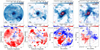 |
Fig. 1 First and second columns: Moment maps of LAsMA 12CO (3–2) and 13CO (3–2) emission. The radius of the entire region is 0.1° (~6.28 pc). The big red circle marks the region with a 0.05° (~3.14 pc) radius, and the small red circle shows the region with a 0.01° (~0.63 pc) radius. Third and fourth columns: moment maps of ALMA 7 m+12 m HCO+ J = 1–0 and H13CO+ J = 1–0 emission. The radius of the entire region is 0.01° (~0.63 pc). Red contours in panels c and d show the 3 mm continuum emission. Black contours in the second row show ATLASGAL 870 µm continuum emission. Dashed black lines in panels b1 and d1 show the paths of the PV diagrams in Fig. 4. Ellipses in panel d represent the dendrogram structures identified in Sect. 3.3. |
2 Observations and data
2.1 LAsMA data
The seven pixel Large APEX sub-Millimeter Array (LAsMA) receiver of the APEX telescope was used to observe the J = 3–2 transitions of 12CO and 13CO in the G333 molecular cloud complex. A detailed description of data calibration, imaging, and product creation procedures is presented in Zhou et al. (2023). The final data cubes have a velocity resolution of 0.25 km s−1 and an angular resolution of 19.5″ and the pixel size is 6″. The final noise levels of the 12CO (3–2) and 13CO (3–2) data cubes are ~0.32 K and ~0.46 K, respectively. In this paper, we only focus on the subregion G332.83-0.55.
2.2 ALMA data
We selected one source from the ATOMS survey (Project ID: 2019.1.00685.S; PI: Tie Liu). The details of the 12 m array and 7 m array ALMA observations were summarized in Liu et al. (2020b, 2021a). Calibration and imaging were carried out using the CASA software package version 5.6 (McMullin et al. 2007); more details can be found in Zhou et al. (2021). All images have been primary-beam corrected. The continuum image reaches a typical 1σ rms noise of ~0.2 mJy in a synthesized beam FWHM size of ~2.2″. In this work, we also use the H13CO+ J = 1–0 and HCO+ J =1–0 molecular lines. The final noise levels of the H13 CO+ J = 1–0 and HCO+ J = 1–0 data cubes are ~0.008 Jy beam−1 and ~0.012 Jy beam−1, respectively.
2.3 Archival data
We also used ATLASGAL+Planck 870 µm data (ATLASGAL combined with Planck data), which are sensitive to a wide range of spatial scales at a resolution of ~21″ (Csengeri et al. 2016).
3 Results
3.1 Connection of gas inflows in LAsMA and ALMA observations
Moment maps of various molecular lines are shown in Fig. 1. The Moment 0 maps of 13CO (3–2), H13CO+ J = 1–0, and HCO+ J =1–0 emission show a typical hub-filament morphology. The FILFINDER algorithm (Koch & Rosolowsky 2015) was used to identify and characterize filaments traced by H13 CO+ (1–0) and 13CO (3–2) emission. Following the method described in Zhou et al. (2022, 2023), we used the integrated intensity (Moment 0) maps to identify filaments. The skeletons of the identified filaments, overlaid on the Moment 0 maps in Fig. 2, are highly consistent with the gas structures. We selected the filaments through the redshifted and blueshifted peaks (LAsMA-f3 and ALMA-f3), and extracted the velocity and intensity along the filaments, as shown in Fig. 3.
Figure 4 displays the position-velocity (PV) diagrams along the dashed lines in panels bl and dl of Fig. 1. For H13CO+ J = 1– 0 emission, feedback from the central UC-HII region identified in Zhang et al. (2023) has destroyed the surrounding molecular gas structure (Fig. 1d). Thus, the diagram looks broken, but it still has a clear double-peak velocity structure, indicating that the surrounding gas is still infalling onto the protocluster (Sect. 3.2). In Fig. 4b, the central part of the PV diagram has a similar morphology to Fig. 4a. Large-scale gas structures with clear velocity gradients are connected to the central velocity jump. Correspondingly, large-scale filamentary structures connected to the central clump can be seen in Figs. 1a and b; small-scale filamentary structures down to dense core scales are also presented in Figs. 1c and d. These features indicate that cloud-scale gas inflows extend down to core scales. The inheritance of gas flows on large scales to small scales is clearly visible in Fig. 3c.
Figure 5a displays the PPV map of 13CO (3–2) emission decomposed by the fully automated Gaussian decomposer GAUSSPY+ (Lindner et al. 2015; Riener et al. 2019); the decomposition was carried out in Zhou et al. (2023). We can see a funnel structure that can be a probe of gravitational collapse as discussed in Zhou et al. (2023). At small scales, we can roughly identify a velocity jump comprised of the redshifted and blueshifted peaks in Fig. 2c, which is clearly shown in Fig. 2d, thanks to the higher resolution of the ALMA data.
To conclude, G332.83-0.55 shows at least two levels of hub-filament structures. Figures 1a and b present the first level from cloud to clump scales. The second level from clump to core scales is shown in Figs. 1c and d. In a statistical study of hub-filament systems in Zhou et al. (2022), we found filaments are ubiquitous in proto-clusters, and hub-filament systems are very common from dense core scales (~0.1 pc) to clump and cloud scales (~1–10 pc). These observed features are reproduced in G332.83-0.55 well.
The structures marked by small red circles in Figs. 1a and b present an approximately spherical morphology due to the limited resolution in single-dish observation, usually referred to as a “clump”. However, in the eyes of ALMA, the spherical clump displays anisotropic and filamentary accretion structures (hub-filament) in Figs. 1c and d. Thus, relative to the traditional “infall envelope”, filamentary accretion and inflow structures may be more realistic in high-mass star-forming clumps.
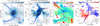 |
Fig. 2 Hierarchical hub-filament structures in G332.83-0.55. (a) and (b) Moment 0 maps of LAsMA 13CO (3–2) and ALMA H13CO+ (1–0) emission. (c) and (d) Moment 1 maps of LAsMA13 CO (3–2) and ALMA H13CO+ (1–0) emission. The hub region marked by a red circle in panels a and c are enlarged in panels b and d. More detailed structures can be seen in panels b and d, thanks to the high resolution of ALMA observation. Lines in color present the filament skeletons identified by the FILFINDER algorithm. |
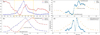 |
Fig. 3 (a) Normalized velocity and intensity along the filament LAsMA-f3 in Fig. 2a; here we can see a blueshifted V-shape velocity structure. (b) Segment of panel a around the central hub; here we can see a V+Λ-shape velocity structure. (c) and (d) Velocity and intensity along the segment of LAsMA-f3 in panel b compared to the velocity and intensity along the filament ALMA-f3 in Fig. 2b. |
 |
Fig. 4 PV diagrams of ALMA H13CO+ (1–0) and LAsMA 13CO (3–2) along the paths marked in Figs. 1d1 and bl. |
3.2 Infall+rotation motions
In Figs. 1c and d, on small scales, H13CO+ J = 1–0 and HCO+ J = 1–0 emission present spiral-like structures, indicating the rotation of gas around the protocluster. PV diagrams in Fig. 4 also reveal rotation motions. The PV diagrams show two peaks separated by several km s−1, and they are symmetrically located with respect to the gravitational center. The double-peaked feature on the PV map is often seen in cluster-forming clumps, and this feature can only be reproduced when the clump has both infall motion and rotation at the same time, thus strongly implying that the clump is collapsing with rotation (Ohashi et al. 1997; Shimoikura et al. 2016, 2018, 2022; Sanna et al. 2019; Liu et al. 2020a). Around the gravitational center, we can see the blueshifted and redshifted extrema at the end of the velocity jump in Fig. 3, which is comparable with Fig. 2 of Sakai et al. (2014). In the schematic diagram of an infalling and rotating envelope model for IRAS 04368+2557 (Sakai et al. 2014), the shift of blueshifted and redshifted peaks can be used to estimate the radius of the centrifugal barrier rc, where the rotation velocity Vrotation has its maximum value. According to Eqs. (1) and (2) in Sakai et al. (2014), we can estimate the mass of the gravitational center according to rc by
 (1)
(1)
The initial physical quantities in this equation can be estimated from the velocity jump in Fig. 3.
Both the velocity fields traced by LAsMA and ALMA data show a velocity jump around the gravitational center. In Fig. 3c, the velocity fields along the large- and small-scale filaments can be roughly connected, despite the significant differences in their resolutions (2.5″ and 19.5″). According to the velocity difference and the separation between blueshifted and redshifted peaks in Fig. 3c, we roughly estimate Vrotation,ALMA ≈ 3.29 km s−1 and rc,ALMA ≈ 0.21 pc. Then according to Eq. (1), the mass of the gravitational center (i.e., the protocluster) is ~264 M⊙.
As a further test, following the method described in Kauffmann et al. (2008), the mass can be computed by dust emission using
 (2)
(2)
where the opacity is
 (3)
(3)
and β is the dust emissivity spectral index. Here, we consider β = 1.5, Fν is the total flux of 3 mm dust emission, d is the distance to the source, and λ is the wavelength. The temperature T takes the value ~31.4 K listed in Table A.1 of Liu et al. (2020b). A mass ~264 M⊙ corresponds to the flux of 3 mm dust emission ~0.12 Jy. This value is ~3% of the total flux of 3 mm continuum emission in ALMA observations. As discussed in Keto et al. (2008) and Zhang et al. (2023), 3 mm continuum emission of UC HII regions in high-resolution interferometric observations should be mostly free–free emission rather than from dust, and thus the proportion of ~3% for the dust emission is reasonable.
3.3 Local dense gas structures
The issues of identifying the structures in a PPV cube by the dendrogram algorithm are described in Zhou et al. (2024b), and thus we adopted the same method as in Zhou et al. (2024a,b) to identify dense gas structures. We directly identified hierarchical (sub)structures based on the 2D integrated intensity (Moment 0) map of H13CO+ (1–0) emission, and then extracted the average spectrum of each structure to investigate its velocity components and gas kinematics. More details can be found in Zhou et al. (2024a). In this work, we focus on leaf structures, which are local gravitational centers. According to their averaged spectra, the structures with absorption features were eliminated first. Following Zhou et al. (2024a), we only consider type 1 (single velocity component) and type 3 (blended velocity component) structures, as marked in Fig. 1d by ellipses.
We derived the column density by combining H13CO+ J = 10 and HCO+ J = 1–0 emission using the same method described in Sect. 3.3 of Zhou et al. (2024a) by the local thermodynamic equilibrium (LTE) analysis. Then the masses and virial ratios of all leaf structures were calculated.
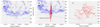 |
Fig. 5 Linkage of large- and small-scale velocity fields in PPV space. (a) Velocity field revealed by LAsMA data 13CO (3–2) on large scales decomposed by GAUSSPY+. (b) Combined velocity fields traced by 13CO (3–2) and H13CO+ (1–0) at different scales, i.e., panel a plus panel c. (c) Velocity field revealed by ALMA data H13CO+ (1–0) on small scales decomposed by GAUSSPY+. |
3.4 Shear and tide from the protocluster
The very large velocity difference (velocity jump) around the protocluster in Figs. 3–5 may indicate that the surrounding gas structures bear considerable shear and tides from the protoclus-ter, apart from infall and rotation motions. Figure 6c shows the scaling relations between the velocity dispersion σ, the effective radius R, and the column density N of all leaf structures, similar to Zhou et al. (2024a,b), the slope of the σs − N * R relation is ∼0.2, which is much smaller than 0.5 and may indicate a pure free-fall gravitational collapse is slowing down.
To investigate the shear and tides from the protocluster, here we analogy to the methods that are adopted on galaxy-cloud scales. For cloud-scale gas structures in the galaxy, as described in Hunter et al. (1998) and Dib et al. (2012), the shear parameter Sg is defined as
 (4)
(4)
We note that Σ is the local gas surface density and Σcri is the critical surface density, which represents the minimal surface density needed to resist the shear. Following Eq. (7) of Dib et al. (2012),
 (5)
(5)
The C represents the density contrast between leaf structures and their surroundings. The ratio between the average surface density derived from 13CO (3 – 2) emission in the FOV of the ALMA observation and the highest surface density of leaf structures is ∼100, and thus we consider C = 100. We note that σ is the local gas velocity dispersion and A is the Oort constant, which measures the local shear level. For a spherical cloud of radius r, with a rotational velocity V at a galactocentric distance RG, A can be calculated as
 (6)
(6)
in the context of molecular clouds, V is determined by the rotation curve of the galaxy. In our case, for gas structures in the clump around the protocluster, V was estimated by the Kepler rotation curve, as discussed in Sect. 3.2. The  , with M0 being the mass of the protocluster and R′ being the distances between gas structures and the protocluster. Shear is effective at tearing apart the gas structure if Sg > 1 and it can be ineffective if Sg < 1.
In a galactic context, the overall gas and stellar distribution can contribute to confine or disrupt the gas structures. For a cloud at a distance RG from the galactic center, the edge of the cloud from the galactic center is at a distance of RG+r. The tidal acceleration in the cloud is ∼ T * r, following Stark & Blitz (1978),
 (7)
(7)
Inserting the Keplerian rotation curve, T = 3GM0/R′3, which is similar to Eq. (8). Then the effective velocity dispersion from the tide for a structure is  , where R is the effective radius of the structure.
In Fig. 6, Sg << 1 and  ; except for two structures adjacent to the protocluster, the results seem to deny the importance of the shear and tide from the protocluster. However, the analysis here is actually not entirely appropriate. For a leaf structure, it also bears the tides from other gas structures, not only the protocluster. In fact, it should be N-body tidal interactions; therefore, a complete tidal calculation would be more appropriate.
3.5 Tidal field
To fully consider the tidal interactions, we directly derived the tidal field according to the density distribution. Only the projected surface density map is available in the observations. To align with other projected physical quantities derived from the observations, we also calculated the 2D projected tide. We note that 3D calculations can refer to Ganguly et al. (2024) and Li (2024). Calculating the gravitational potential field ϕ(x, y) based on the surface density map Σ(x, y) has been discussed in Gong & Ostriker (2011); He et al. (2023). The tidal tensor described in Appendix A has only two eigenvalues in the case of 2D, that is to say λi (i = 1,2). As described in Appendix A, the tidal tensor of a structure includes both self-gravity and external tides, that is, T = Text + Tint. The decomposition of the tidal tensor is discussed in detail in Appendix A. For three limiting cases, the external tides can be measured by λ1, λ2, and (λ2 − λ1)/2 and they are called Td,1, Td,2, and Td,3, respectively. Figure 7 displays different components of the tidal tensor.
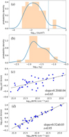 |
Fig. 6 (a) Distribution of the shear parameter S𝑔 .(b) Distribution of the velocity dispersion ratio between σt and σ. (c) σ − N * R relation, where σ is the local gas velocity dispersion. (d) σs − N * R relation, where |

3.6 Structure of G332.83-0.55
As shown in Fig. 1 of Zhou et al. (2023), G332.83-0.55 is part of a large-scale shell structure. Thus, it may have a sheet structure. In combining Figs. 1b and 5a, the single direction gas inflows on large scales also indicate that the structure on large scales should be approximately 2D, and should be face-on. Thus, we can observe the unidirectional converging flows. Close to the center, the structure becomes thicker and thicker. The redshifted and blueshifted components may originate from the forward and backward gas motions in the hub region. However, strong rotation motions on small scales may also explain their origin. The 3D and 2D structures of G332.83-0.55 may not be very different, given its limited thickness. Therefore, 2D-projected tidal field strength should be comparable to those for 3D ones, and Eq. (A.8) derived from the 3D tidal tensor in Appendix A should still be effective for a 2D situation, which is confirmed in Fig. 8a.
3.7 Pixel-by-pixel computation
Below we explain how we tested the above tidal tensor analysis using an original method.
3.7.1 Maximum computation
For a structure A, located at a distance R from the center of another structure B, of mass M, the tidal strength sustained by structure A due to the external gravity from structure B is
 (8)
(8)
The total tidal strength at a pixel measures the total deformation due to the external tides at that point. A gas structure is neither a rigid body nor point mass, but it is a parcel of gas with malleability. Most gas structures are also not spherically symmetric, and their morphologies can be highly complex. Although the external gravity from all directions may cancel each other out in a structure, the tides inside the structure due to the external gravity do not. Therefore, we used the scalar superposition to measure the overall tidal strength in the structure from the external gravity. Tidal tearing may be an important cause for the deformation and complex morphology of gas structures, as discussed in Sect. 4.1.
Using the mask of the dendrogram structure, we divided the density map into two parts, that is, the structure itself and all other materials apart from this structure. For the external tides from all outside material sustained by a point in structure A, a simple calculation involves using Eq. (8) to directly calculate the tidal strength at that point pixel by pixel, as illustrated in Fig. 9b. The average tidal strength of all the pixels in structure A can then represent the average tidal strength sustained by the structure.
3.7.2 Minimal computation
As illustrated in Fig. 9b, the above computation is limited to a 2D plane. In Eq. (8), the tidal strength is very sensitive to the distance. If the external structure and the calculated structure are not in the same plane, the 2D calculation underestimates the distance between them and thus overestimates the tidal strength (maximum computation, Tmax). However, we only have the 2D projection in the observation. The 3D structure of the molecular gas is unknown, but we can consider an extreme case. Using the average effective radius (~0.03 pc) of all leaf structures as the characteristic scale height of G332.83-0.55, all external material apart from the calculated structure was moved vertically to 0.03 pc away, as illustrated in Fig. 10c. This is unrealistic, given the continuity of the matter distribution in a cloud. As a limiting case, the estimated tidal strength should be smaller than the actual value (minimal computation, Tmin,s).
The other minimal computation (Tmin,v) is the vector superposition of tides, which allows the tidal interactions to directly cancel each other out. Using the calculated point in the target structure as the coordinate origin to build a 2D coordinate system, all external tides were decomposed to the coordinate axes.
Then we calculated the overall tidal strength at the calculated point after performing vector superposition along each axis.
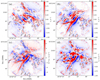 |
Fig. 7 Different components of the projected tidal field in the FOV of the ALMA observation. |
3.7.3 Tide from the envelope
As shown in Fig. 2, the dendrogram structures are embedded in a larger-scale gas environment. The material outside of the FOV of ALMA observation may also produce considerable external tides (Tout) on small-scale dendrogram structures. Using the H2 column density derived from ATLASGAL+Planck 870 µm in Zhou et al. (2024b), the matter in the FOV of ALMA observation was first masked, as shown in Fig. 9a. Then we calculated the external tides at each pixel in the FOV. The averaged tidal strength of all pixels is ~1.4 × 10− 25 s− 2. Compared with the tidal strength in Fig. 8b, Tout is very small and therefore can be ignored.
3.7.4 Comparison
Figure 8b shows that the components Td,1, Td,2, and Td,3 (whose derivation is detailed in Appendix A) are comparable. Especially, they are also comparable with Tmin,s and Tmin,v. As expected, Tmax is significantly larger than others. For Td,1, Td,2, T d, 3, Tmin,s, and Tmin,v, Tmin,v is slightly larger than others and the value of is in the middle. As a compromise, we use the value of Tmin,s to represent the external tides in the subsequent analysis.
4 Discussion
4.1 Tide-regulated gravitational collapse
The average strength of the external tides Tmin,s of a structure was used to measure the deformation of the structure due to the external gravity. The effective velocity dispersion from the external tides of the structure is  , and the corresponding energy
 (9)
(9)
The gravitational potential energy Eg and internal kinetic energy Ek were calculated in the same way as presented in Zhou et al. (2024b).
The slowing down of a pure free-fall gravitational collapse as revealed by the shallow σs − N * R relation means that there are some physical processes working against gravitational collapse, such as tidal tearing from external gravity. The effect of the external tides on the gravitational collapse of gas structures can also be reflected in the scaling relation. After adding the contribution of the tidal interactions to the observed velocity dispersion, the effective velocity dispersion  , then the σs − N * R relation was fitted again. As shown in Fig. 6d, now the slope is close to 0.5, and the correlation also gets stronger. Thus, the deformation due to the external tides may effectively slow down the pure free-fall gravitational collapse of gas structures.
However, as shown in Fig. 11a, the sum of Ek and Et is notably larger than Eg. The external tidal strength may be overestimated. The velocity dispersion is a manifestation of gas perturbations due to many physical processes, including gravitation collapse, tidal tearing, and turbulence. Thus, Ek should be overestimated. Moreover, when Ek + Et > Eg, it does not mean that the structure cannot be gravitationally bound. A structure is deformed by external tides from the surrounding material, and at the same time, the surrounding material also provides the structure with a confining pressure.
Previous studies have suggested that the external pressure provided by the larger-scale molecular gas might help to confine dense structures in molecular clouds (Spitzer 1978; McKee 1989; Elmegreen 1989; Ballesteros-Paredes 2006; Kirk et al. 2006, 2017; Dib et al. 2007; Lada et al. 2008; Pattle et al. 2015; Li et al. 2020; Zhou et al. 2024b). External pressure can have various origins; here we mainly consider the external pressure from the ambient cloud for each decomposed structure using
 (10)
(10)
where Pcl is the gas pressure,  is the mean surface density of the cloud, and Σr is the surface density at the location of each structure (McKee 1989; Kirk et al. 2017). The external pressure energy can be calculated as
 (11)
(11)
As shown in Fig. 11b, after considering the external pressure, Ek + Et < Eg + Ep. The external tide tries to tear up the structure, but the external pressure on the structure prevents this process from occurring. The counterbalance between the external tide and external pressure hinders the gravitational collapse of the structure, which can also cause a pure free-fall gravitational collapse to slow down.
Gravity can play multiple roles in cloud evolution. Inside dense regions, it drives fragmentation and collapse, and outside these regions, it can suppress the low-density gas from collapsing through extensive tidal forces and drive accretion (Li 2024). This work confirms that tidal interactions can significantly influence the dynamics and kinematics of gas structures and regulate their gravitational collapse. In Figs. 14c and 15c of Zhou et al. (2024b), in the G333 complex, for 3608 gas structures on cloud-clump scales, the slopes of the σ − N * R relations are ~0.19 and ~0.26, respectively. In Fig. 5a of Zhou et al. (2024a), for 2420 dense gas structures on clump-core scales in 64 ATOMS sources (clumps) at different evolutionary stages, the slope of the σ − N * R relation is ~0.27. According to the above analysis, these shallow slopes (significantly smaller than 0.5) may indicate extensive tide-regulated gravitational collapse from cloud to core scales, which will be discussed in detail in future work.
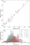 |
Fig. 8 (a) Comparison of Ea,int and Eg of dendrogram structures. (b) Distribution of the average tidal strength in each computation. |
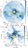 |
Fig. 9 Computed structure first masked from the density map. The external tides from all outside material sustained by a point in the computed structure was calculated pixel by pixel and is illustrated by orange lines. (a) Background representing the column density map derived from ATLASGAL+Planck 870 µm data. The material in the FOV of the ALMA observation (white region) was masked. (b) Background representing the column density map derived from H13CO+ J = 1−0 and HCO+ J = 1−0 lines from the ALMA observation by the LTE analysis. |
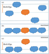 |
Fig. 10 Edge-on view of G332.83-0.55. The calculated gas structure is in red, and all external material apart from the calculated structure is in blue. (a) The gas distribution in G332.83-0.55 can be everywhere. (b) In 2D computation, all molecular gases are assumed to be concentrated on the same plane. Thus, we obtained a maximal estimate for the tidal strength. (c) Taking a characteristic scale height of the molecular gas as 0.03 pc, all external material apart from the calculated structure were moved vertically to 0.03 pc away. Thus we obtained a minimal estimate of the tidal strength. |
4.2 Gravitational focusing
In Figs. 4b and 5b, on large scales, the funnel structure is consistent with the schematic diagram in Fig. 9 of Zhou et al. (2023). However, it looks as though the bottom of the funnel splits into two parts in Figs. 4b and 5b. A velocity jump appears in the center comprised of the redshifted and blueshifted components, which may be attributed to the infalling and rotating motions around the protocluster. If we turn over the redshifted component and let it merge with the blueshifted component, then we obtain the funnel structure in Fig. 9 of Zhou et al. (2023).
Similar to lights converging to the focus, now the gas inflows are converging to the gravitational center, that is, the hub region of G332.83-0.55. Thus, there is a vivid “gravitational focusing” process, which also provides a clue as to the formation of the hub-filament structure. As shown in Fig. 1 of Zhou et al. (2023), the entire G333 complex has a large-scale shell structure. G332.83-0.55 is a fragment on the shell, which should have a sheet configuration initially; for more details, readers can also refer to Sect. 3.6. Then the subsequent gravitational focusing process yields the hub-filament structure. In Fig. 1b, the hub-filament structure is decoupling from the surrounding gas environment due to gravitational collapse.
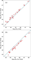 |
Fig. 11 Comparison between the structural energies, i.e., the gravitational potential energy Eg, the kinetic energy Ek, the tidal energy Et, and the external pressure energy Ep. |
5 Summary
- 1.
In high-resolution APEX/LAsMA 12CO and 13CO (3-2) observations, G332.83-0.55 has a clear hub-filament morphology at ~10 pc, and its hub corresponds to the ATLASGAL clump AGAL332.826-00.549. We zoomed in on the hub region of G332.83-0.55 using higher-resolution ALMA HCO+ (1−0) and H13CO+ (1−0) observations, and found that it still presents a hub-filament structure. Thus, G332.83-0.55 contains at least two levels of hub-filament structures. High-resolution single-dish and ALMA observations provide the opportunity to trace gas inflows from cloud to core scales.
- 2.
G332.83-0.5 is collapsing with rotation. Around the gravitational center (i.e., the protocluster), both the velocity fields traced by LAsMA and ALMA observations show velocity jumps comprised of redshifted and blueshifted peaks. According to the velocity difference and the separation between blueshifted and redshifted peaks, we roughly estimated the rotation velocity Vrotatio,ALMA ≈ 3.29 km s− 1 and the centrifugal barrier rc,ALMA ≈ 0.21 pc. Then the mass of the gravitational center (i.e., the protocluster) was estimated to be ≈264 M⊙, which agrees with the mass estimated by 3 mm dust emission.
- 3.
We directly identified local dense gas structures based on the 2D integrated intensity (Moment 0) map of H13CO+ J = 1−0 emission using the dendrogram algorithm, and then extracted the average spectra to fit the velocity dispersion. The slope of the σ − N * R relation for leaf structures is ~0.2, which is much smaller than 0.5 of the pure free-fall gravitational collapse. This may indicate that a pure free-fall gravitational collapse is slowing down.
- 4.
We investigated the effect of shear and tides from the protocluster on the surrounding local dense gas structures. The results seem to deny the importance of shear and tides from the protocluster. However, for a gas structure, it also bears the tides from other gas structures and the general gas distribution, not only the protocluster. To fully consider the tidal interactions, we derived the tide field according to the density distribution, and then used the average strength of the external tides of a structure to measure the total tidal interactions on the structure. For comparison, we also adopted an original pixel-by-pixel computation to estimate the average tidal strength of each structure. Both methods give comparable calculation results.
- 5.
After considering the tidal interactions for all structures, the slope of the σ − N * R relation is close to 0.5, and the correlation also gets stronger. Thus, the deformation due to the external tides can effectively slow down the pure free-fall gravitational collapse of gas structures. The external tide tries to tear up the structure, but the external pressure on the structure prevents this process from occurring. The counterbalance between an external tide and external pressure hinders the free-fall gravitational collapse of the structure, which can also cause a pure free-fall gravitational collapse to slow down. These mechanisms can be called “tide-regulated gravitational collapse”.
Acknowledgements
This publication is based on data acquired with the Atacama Pathfinder Experiment (APEX) under programme ID M-0109.F-9514A-2022. APEX has been a collaboration between the Max-Planck-Institut für Radioastronomie, the European Southern Observatory, and the Onsala Space Observatory. This research made use of astrodendro, a Python package to compute dendrograms of Astronomical data (http://www.dendrograms.org/). This paper makes use of the following ALMA data: ADS/JAO.ALMA#2019.1.00685.S. ALMA is a partnership of ESO (representing its member states), NSF (USA) and NINS (Japan), together with NRC (Canada), MOST and ASIAA (Taiwan), and KASI (Republic of Korea), in cooperation with the Republic of Chile. The Joint ALMA Observatory is operated by ESO. T.L. acknowledges the supports by the National Key R&D Program of China (No. 2022YFA1603101), National Natural Science Foundation of China (NSFC) through grants No.12073061 and No.12122307, the international partnership program of Chinese Academy of Sciences through grant No.114231KYSB20200009, and the Tianchi Talent Program of Xinjiang Uygur Autonomous Region.
Appendix A Tidal tensor
For a gravitational potential field Φ, the tidal tensor T is defined as
 (A.1)
(A.1)
The eigenvalues of the tidal tensor contain information regarding the extent of deformation (compression and disruption) experienced at a specific point due to the local gravitational field. The diagonalized tidal tensor is given as
![Mathematical equation: ${\bf{T}} = \left[ {\matrix{ {{\lambda _1}} & 0 & 0 \cr 0 & {{\lambda _2}} & 0 \cr 0 & 0 & {{\lambda _3}} \cr } } \right].$](/articles/aa/full_html/2024/06/aa49514-24/aa49514-24-eq20.png) (A.2)
(A.2)
The sign of the eigenvalues (λ1, λ2, and λ3) indicates whether the given mode is compressive (λi > 0) or disruptive (λi < 0), while the magnitude represents the strength of the respective compressive and disruptive mode. The trace of the tidal tensor  contains the local density information in the Poisson equation:
 (A.3)
(A.3)
This indicates that the trace is zero when the location where the tidal tensor is assessed lies outside the distribution of mass.
As was done in Ganguly et al. (2024), the tidal tensor can be split into three parts: the tidal tensor due to only the matter inside the structure, Tint, and into a second component due only to the matter distribution external to the structure, Text. Their sum, due to the entire matter distribution,
 (A.4)
(A.4)
Here, T represents the net deformation due to both the structure itself and its surroundings. We note that Text represents the deformation introduced solely due to the external materials. The trace of the three parts are the following:
 (A.5)
(A.5)
 (A.6)
(A.6)
 (A.7)
(A.7)
where ρa is the average density of the structure with radius R and total mass M, ρa = M/(4/3πR3).
According to Tr(Tint) = 4πGρa, the corresponding energy can be estimated by
 (A.8)
(A.8)
Thus, the tidal tensor Tint represents the self-gravity of the structure. If we want to estimate the tidal interactions from all external materials on the structure, we should focus on Text.
The trace in equation.A.7 indicates that Text due to only matter distribution external to the structure must contain both compressive and disruptive modes, corresponding to positive and negative λi, respectively. In contrast, Tint due to only the matter inside the structure and T due to the entire matter distribution must contain at least one compressive mode, but it might also be fully compressive. These rules are also applicable for 2D projected tidal tensor. According to equation.A.4, the 2D tidal tensor can be decomposed as
![Mathematical equation: $\left[ {\matrix{ {{\lambda _1}} & 0 \cr 0 & {{\lambda _2}} \cr } } \right] = \left[ {\matrix{ { - {A_0}} & 0 \cr 0 & {{A_0}} \cr } } \right] + \left[ {\matrix{ {{A_1}} & 0 \cr 0 & {{A_2}} \cr } } \right]; $](/articles/aa/full_html/2024/06/aa49514-24/aa49514-24-eq28.png) (A.9)
(A.9)
assuming A2 = k * A1, we have  , and
, and  . There are three cases:
- (1)
When k = 1,
 (Fig.7(c)).
 - (2)
When k << 1, A1 ≈ λ1 + λ2, A2 ≈ 0, A0 ≈ λ2 (Fig.7(b)).
- (3)
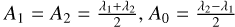
When k >> 1, A1 ≈ 0, A2 ≈ λ1 + λ2, A0 ≈ −λ1 (Fig.7(a)). We estimated the averaged strength of the external tidal field for each structure according to Fig.7(a), (b) and (c), that is, the averaged value of |A0, a| in each structure. As shown in Fig.8(b), the three cases give similar estimates of the averaged strength of the external tidal field.
References
- Ballesteros-Paredes, J. 2006, MNRAS, 372, 443 [NASA ADS] [CrossRef] [Google Scholar]
- Chen, X., Sobolev, A. M., Ren, Z.-Y., et al. 2020, Nat. Astron., 4, 1170 [Google Scholar]
- Contreras, Y., Garay, G., Rathborne, J. M., & Sanhueza, P. 2016, MNRAS, 456, 2041 [CrossRef] [Google Scholar]
- Csengeri, T., Weiss, A., Wyrowski, F., et al. 2016, A&A, 585, A104 [NASA ADS] [CrossRef] [EDP Sciences] [Google Scholar]
- Dewangan, L. K., Ojha, D. K., Sharma, S., et al. 2020, ApJ, 903, 13 [Google Scholar]
- Dib, S. 2023, MNRAS, 524, 1625 [NASA ADS] [CrossRef] [Google Scholar]
- Dib, S., Kim, J., Vázquez-Semadeni, E., Burkert, A., & Shadmehri, M. 2007, ApJ, 661, 262 [NASA ADS] [CrossRef] [Google Scholar]
- Dib, S., Helou, G., Moore, T. J. T., Urquhart, J. S., & Dariush, A. 2012, ApJ, 758, 125 [NASA ADS] [CrossRef] [Google Scholar]
- Elmegreen, B. G. 1989, ApJ, 338, 178 [NASA ADS] [CrossRef] [Google Scholar]
- Ganguly, S., Walch, S., Clarke, S. D., & Seifried, D. 2024, MNRAS, 528, 3630 [NASA ADS] [CrossRef] [Google Scholar]
- Gong, H., & Ostriker, E. C. 2011, ApJ, 729, 120 [NASA ADS] [CrossRef] [Google Scholar]
- He, Z.-Z., Li, G.-X., & Burkert, A. 2023, MNRAS, 526, L20 [NASA ADS] [CrossRef] [Google Scholar]
- Henshaw, J. D., Caselli, P., Fontani, F., Jiménez-Serra, I., & Tan, J. C. 2014, MNRAS, 440, 2860 [Google Scholar]
- Hunter, D. A., Elmegreen, B. G., & Baker, A. L. 1998, ApJ, 493, 595 [NASA ADS] [CrossRef] [Google Scholar]
- Issac, N., Tej, A., Liu, T., et al. 2019, MNRAS, 485, 1775 [NASA ADS] [CrossRef] [Google Scholar]
- Izquierdo, A. F., Galván-Madrid, R., Maud, L. T., et al. 2018, MNRAS, 478, 2505 [NASA ADS] [CrossRef] [Google Scholar]
- Kauffmann, J., Bertoldi, F., Bourke, T. L., Evans, N. J., I., & Lee, C. W. 2008, A&A, 487, 993 [NASA ADS] [CrossRef] [EDP Sciences] [Google Scholar]
- Keto, E., Zhang, Q., & Kurtz, S. 2008, ApJ, 672, 423 [NASA ADS] [CrossRef] [Google Scholar]
- Kirk, H., Johnstone, D., & Di Francesco, J. 2006, ApJ, 646, 1009 [Google Scholar]
- Kirk, H., Friesen, R. K., Pineda, J. E., et al. 2017, ApJ, 846, 144 [Google Scholar]
- Koch, E. W., & Rosolowsky, E. W. 2015, MNRAS, 452, 3435 [Google Scholar]
- Kumar, M. S. N., Palmeirim, P., Arzoumanian, D., & Inutsuka, S. I. 2020, A&A, 642, A87 [EDP Sciences] [Google Scholar]
- Lada, C. J., Muench, A. A., Rathborne, J., Alves, J. F., & Lombardi, M. 2008, ApJ, 672, 410 [Google Scholar]
- Li, G.-X. 2024, MNRAS, 528, L52 [Google Scholar]
- Li, S., Zhang, Q., Liu, H. B., et al. 2020, ApJ, 896, 110 [Google Scholar]
- Lindner, R. R., Vera-Ciro, C., Murray, C. E., et al. 2015, AJ, 149, 138 [NASA ADS] [CrossRef] [Google Scholar]
- Liu, H. B., Galván-Madrid, R., Jiménez-Serra, I., et al. 2015, ApJ, 804, 37 [Google Scholar]
- Liu, T., Zhang, Q., Kim, K.-T., et al. 2016, ApJ, 824, 31 [Google Scholar]
- Liu, S.-Y., Su, Y.-N., Zinchenko, I., et al. 2020a, ApJ, 904, 181 [Google Scholar]
- Liu, T., Evans, N. J., Kim, K.-T., et al. 2020b, MNRAS, 496, 2790 [Google Scholar]
- Liu, H.-L., Liu, T., Evans, Neal J., I., et al. 2021a, MNRAS, 505, 2801 [NASA ADS] [CrossRef] [Google Scholar]
- Liu, X.-L., Xu, J.-L., Wang, J.-J., et al. 2021b, A&A, 646, A137 [NASA ADS] [CrossRef] [EDP Sciences] [Google Scholar]
- Liu, H.-L., Tej, A., Liu, T., et al. 2022, MNRAS, 511, 4480 [NASA ADS] [CrossRef] [Google Scholar]
- Liu, H.-L., Tej, A., Liu, T., et al. 2023, MNRAS, 522, 3719 [NASA ADS] [CrossRef] [Google Scholar]
- Lu, X., Zhang, Q., Liu, H. B., et al. 2018, ApJ, 855, 9 [Google Scholar]
- Maud, L. T., Hoare, M. G., Galván-Madrid, R., et al. 2017, MNRAS, 467, L120 [NASA ADS] [Google Scholar]
- McKee, C. F. 1989, ApJ, 345, 782 [NASA ADS] [CrossRef] [Google Scholar]
- McMullin, J. P., Waters, B., Schiebel, D., Young, W., & Golap, K. 2007, ASP Conf. Ser., 376, 127 [Google Scholar]
- Motte, F., Bontemps, S., & Louvet, F. 2018, ARA&A, 56, 41 [NASA ADS] [CrossRef] [Google Scholar]
- Myers, P. C. 2009, ApJ, 700, 1609 [Google Scholar]
- Ohashi, N., Hayashi, M., Ho, P. T. P., & Momose, M. 1997, ApJ, 475, 211 [NASA ADS] [CrossRef] [Google Scholar]
- Olguin, F. A., Sanhueza, P., Chen, H.-R. V., et al. 2023, ApJ, 959, L31 [NASA ADS] [CrossRef] [Google Scholar]
- Pattle, K., Ward-Thompson, D., Kirk, J. M., et al. 2015, MNRAS, 450, 1094 [NASA ADS] [CrossRef] [Google Scholar]
- Peretto, N., Fuller, G. A., Duarte-Cabral, A., et al. 2013, A&A, 555, A112 [NASA ADS] [CrossRef] [EDP Sciences] [Google Scholar]
- Riener, M., Kainulainen, J., Henshaw, J. D., et al. 2019, A&A, 628, A78 [NASA ADS] [CrossRef] [EDP Sciences] [Google Scholar]
- Sakai, N., Sakai, T., Hirota, T., et al. 2014, Nature, 507, 78 [Google Scholar]
- Sanhueza, P., Girart, J. M., Padovani, M., et al. 2021, ApJ, 915, L10 [NASA ADS] [CrossRef] [Google Scholar]
- Sanna, A., Kölligan, A., Moscadelli, L., et al. 2019, A&A, 623, A77 [NASA ADS] [CrossRef] [EDP Sciences] [Google Scholar]
- Schneider, N., Csengeri, T., Hennemann, M., et al. 2012, A&A, 540, L11 [NASA ADS] [CrossRef] [EDP Sciences] [Google Scholar]
- Shimoikura, T., Dobashi, K., Matsumoto, T., & Nakamura, F. 2016, ApJ, 832, 205 [NASA ADS] [CrossRef] [Google Scholar]
- Shimoikura, T., Dobashi, K., Nakamura, F., Matsumoto, T., & Hirota, T. 2018, ApJ, 855, 45 [NASA ADS] [CrossRef] [Google Scholar]
- Shimoikura, T., Dobashi, K., Hirano, N., et al. 2022, ApJ, 928, 76 [NASA ADS] [CrossRef] [Google Scholar]
- Spitzer, L. 1978, Physical Processes in the Interstellar Medium (Hoboken: Wiley) [Google Scholar]
- Stark, A. A., & Blitz, L. 1978, ApJ, 225, L15 [NASA ADS] [CrossRef] [Google Scholar]
- Vázquez-Semadeni, E., Palau, A., Ballesteros-Paredes, J., Gómez, G. C., & Zamora-Avilés, M. 2019, MNRAS, 490, 3061 [Google Scholar]
- Xu, F.-W., Wang, K., Liu, T., et al. 2023, MNRAS, 520, 3259 [NASA ADS] [CrossRef] [Google Scholar]
- Yang, D., Liu, H.-L., Tej, A., et al. 2023, ApJ, 953, 40 [NASA ADS] [CrossRef] [Google Scholar]
- Yuan, J., Li, J.-Z., Wu, Y., et al. 2018, ApJ, 852, 12 [Google Scholar]
- Zhang, Q., Wang, K., Lu, X., & Jiménez-Serra, I. 2015, ApJ, 804, 141 [Google Scholar]
- Zhang, C., Zhu, F.-Y., Liu, T., et al. 2023, MNRAS, 520, 3245 [NASA ADS] [CrossRef] [Google Scholar]
- Zhou, J.-W., Liu, T., Li, J.-Z., et al. 2021, MNRAS, 508, 4639 [NASA ADS] [CrossRef] [Google Scholar]
- Zhou, J.-W., Liu, T., Evans, N. J., et al. 2022, MNRAS, 514, 6038 [NASA ADS] [CrossRef] [Google Scholar]
- Zhou, J. W., Wyrowski, F., Neupane, S., et al. 2023, A&A, 676, A69 [NASA ADS] [CrossRef] [EDP Sciences] [Google Scholar]
- Zhou, J. W., Dib, S., Wyrowski, F., et al. 2024a, A&A, 682, A173 [NASA ADS] [CrossRef] [EDP Sciences] [Google Scholar]
- Zhou, J. W., Wyrowski, F., Neupane, S., et al. 2024b, A&A, 682, A128 [NASA ADS] [CrossRef] [EDP Sciences] [Google Scholar]
All Figures
|
Fig. 1 First and second columns: Moment maps of LAsMA 12CO (3–2) and 13CO (3–2) emission. The radius of the entire region is 0.1° (~6.28 pc). The big red circle marks the region with a 0.05° (~3.14 pc) radius, and the small red circle shows the region with a 0.01° (~0.63 pc) radius. Third and fourth columns: moment maps of ALMA 7 m+12 m HCO+ J = 1–0 and H13CO+ J = 1–0 emission. The radius of the entire region is 0.01° (~0.63 pc). Red contours in panels c and d show the 3 mm continuum emission. Black contours in the second row show ATLASGAL 870 µm continuum emission. Dashed black lines in panels b1 and d1 show the paths of the PV diagrams in Fig. 4. Ellipses in panel d represent the dendrogram structures identified in Sect. 3.3. |
| In the text | |
|
Fig. 2 Hierarchical hub-filament structures in G332.83-0.55. (a) and (b) Moment 0 maps of LAsMA 13CO (3–2) and ALMA H13CO+ (1–0) emission. (c) and (d) Moment 1 maps of LAsMA13 CO (3–2) and ALMA H13CO+ (1–0) emission. The hub region marked by a red circle in panels a and c are enlarged in panels b and d. More detailed structures can be seen in panels b and d, thanks to the high resolution of ALMA observation. Lines in color present the filament skeletons identified by the FILFINDER algorithm. |
| In the text | |
|
Fig. 3 (a) Normalized velocity and intensity along the filament LAsMA-f3 in Fig. 2a; here we can see a blueshifted V-shape velocity structure. (b) Segment of panel a around the central hub; here we can see a V+Λ-shape velocity structure. (c) and (d) Velocity and intensity along the segment of LAsMA-f3 in panel b compared to the velocity and intensity along the filament ALMA-f3 in Fig. 2b. |
| In the text | |
|
Fig. 4 PV diagrams of ALMA H13CO+ (1–0) and LAsMA 13CO (3–2) along the paths marked in Figs. 1d1 and bl. |
| In the text | |
|
Fig. 5 Linkage of large- and small-scale velocity fields in PPV space. (a) Velocity field revealed by LAsMA data 13CO (3–2) on large scales decomposed by GAUSSPY+. (b) Combined velocity fields traced by 13CO (3–2) and H13CO+ (1–0) at different scales, i.e., panel a plus panel c. (c) Velocity field revealed by ALMA data H13CO+ (1–0) on small scales decomposed by GAUSSPY+. |
| In the text | |
|
Fig. 6 (a) Distribution of the shear parameter S𝑔 .(b) Distribution of the velocity dispersion ratio between σt and σ. (c) σ − N * R relation, where σ is the local gas velocity dispersion. (d) σs − N * R relation, where |
| In the text | |
|
Fig. 7 Different components of the projected tidal field in the FOV of the ALMA observation. |
| In the text | |
|
Fig. 8 (a) Comparison of Ea,int and Eg of dendrogram structures. (b) Distribution of the average tidal strength in each computation. |
| In the text | |
|
Fig. 9 Computed structure first masked from the density map. The external tides from all outside material sustained by a point in the computed structure was calculated pixel by pixel and is illustrated by orange lines. (a) Background representing the column density map derived from ATLASGAL+Planck 870 µm data. The material in the FOV of the ALMA observation (white region) was masked. (b) Background representing the column density map derived from H13CO+ J = 1−0 and HCO+ J = 1−0 lines from the ALMA observation by the LTE analysis. |
| In the text | |
|
Fig. 10 Edge-on view of G332.83-0.55. The calculated gas structure is in red, and all external material apart from the calculated structure is in blue. (a) The gas distribution in G332.83-0.55 can be everywhere. (b) In 2D computation, all molecular gases are assumed to be concentrated on the same plane. Thus, we obtained a maximal estimate for the tidal strength. (c) Taking a characteristic scale height of the molecular gas as 0.03 pc, all external material apart from the calculated structure were moved vertically to 0.03 pc away. Thus we obtained a minimal estimate of the tidal strength. |
| In the text | |
|
Fig. 11 Comparison between the structural energies, i.e., the gravitational potential energy Eg, the kinetic energy Ek, the tidal energy Et, and the external pressure energy Ep. |
| In the text | |
Current usage metrics show cumulative count of Article Views (full-text article views including HTML views, PDF and ePub downloads, according to the available data) and Abstracts Views on Vision4Press platform.
Data correspond to usage on the plateform after 2015. The current usage metrics is available 48-96 hours after online publication and is updated daily on week days.
Initial download of the metrics may take a while.