| Issue |
A&A
Volume 676, August 2023
|
|
|---|---|---|
| Article Number | A69 | |
| Number of page(s) | 23 | |
| Section | Interstellar and circumstellar matter | |
| DOI | https://doi.org/10.1051/0004-6361/202346500 | |
| Published online | 10 August 2023 | |
High-resolution APEX/LAsMA 12CO and 13CO (3–2) observation of the G333 giant molecular cloud complex
I. Evidence for gravitational acceleration in hub-filament systems★
1
Max-Planck-Institut für Radioastronomie,
Auf dem Hügel 69,
53121
Bonn, Germany
e-mail: This email address is being protected from spambots. You need JavaScript enabled to view it.
2
Centre for Astrophysics and Planetary Science, University of Kent,
Canterbury,
CT2 7NH, UK
3
Department of Astronomy, The University of Texas at Austin,
2515 Speedway, Stop C1400, Austin,
Texas
78712-1205, USA
4
Instituto de Radioastronomía y Astrofísica, Universidad Nacional Autónoma de México,
Antigua Carretera a Pátzcuaro # 8701, Ex-Hda. San José de la Huerta, Morelia,
Michoacán,
58089, Mexico
5
Shanghai Astronomical Observatory, Chinese Academy of Sciences,
80 Nandan Road,
Shanghai
200030, PR China
Received:
24
March
2023
Accepted:
17
May
2023
Abstract
Context. Hub-filament systems are suggested to be the birth cradles of high-mass stars and clusters.
Aims. We investigate the gas kinematics of hub-filament structures in the G333 giant molecular cloud complex using 13CO (3–2) observed with the APEX/LAsMA heterodyne camera.
Methods. We applied the FILFINDER algorithm to the integrated intensity maps of the 13CO J = 3–2 line to identify filaments in the G333 complex, and we extracted the velocity and intensity along the filament skeleton from moment maps. Clear velocity and density fluctuations are seen along the filaments, allowing us to fit velocity gradients around the intensity peaks.
Results. The velocity gradients we fit to the LAsMA and ALMA data agree with each other over the scales covered by ALMA observations in the ATOMS survey (<5 pc). Changes in velocity gradient with scale indicate a funnel structure of the velocity field in position-position-velocity (PPV) space. This is indicative of a smooth, continuously increasing velocity gradient from large to small scales, and thus is consistent with gravitational acceleration. The typical velocity gradient corresponding to a 1 pc scale is ~1.6 km s−1 pc−1. Assuming freefall, we estimate a kinematic mass within 1 pc of ~1190 M⊙, which is consistent with typical masses of clumps in the ATLASGAL survey of massive clumps in the inner Galaxy. We find direct evidence for gravitational acceleration from a comparison of the observed accelerations to those predicted by freefall onto dense hubs with masses from millimeter continuum observations. On large scales, we find that the inflow may be driven by the larger-scale structure, consistent with the hierarchical structure in the molecular cloud and gas inflow from large to small scales. The hub-filament structures at different scales may be organized into a hierarchical system extending up to the largest scales probed through the coupling of gravitational centers at different scales.
Conclusions. We argue that the funnel structure in PPV space can be an effective probe for the gravitational collapse motions in molecular clouds. The large-scale gas inflow is driven by gravity, implying that the molecular clouds in the G333 complex may be in a state of global gravitational collapse.
Key words: ISM: kinematics and dynamics / methods: data analysis / ISM: clouds / surveys / stars: formation / submillimeter: ISM
The data are only available at the CDS via anonymous ftp to cdsarc.cds.unistra.fr (130.79.128.5) or via https://cdsarc.cds.unistra.fr/viz-bin/cat/J/A+A/676/A69
© The Authors 2023
 Open Access article, published by EDP Sciences, under the terms of the Creative Commons Attribution License (https://creativecommons.org/licenses/by/4.0), which permits unrestricted use, distribution, and reproduction in any medium, provided the original work is properly cited.
This article is published in open access under the Subscribe to Open model.
Open Access funding provided by Max Planck Society.
1 Introduction
To understand the formation of hierarchical structures in high-mass star formation regions, it is critical to measure the dynamical coupling between density enhancements in giant molecular clouds and the gas motion in their local environment (McKee & Ostriker 2007; Motte et al. 2018; Henshaw et al. 2020). These studies may distinguish between competing concepts for high-mass star formation, such as monolithic collapse of turbulent cores in virial equilibrium (McKee & Tan 2003; Krumholz et al. 2007), competitive accretion in a protocluster environment through Bondi-Hoyle accretion (Bonnell et al. 1997, 2001), turbulence-driven inertial-inflow (Padoan et al. 2020) and gravity-dominated global hierarchical collapse (Vázquez-Semadeni et al. 2009, 2017, 2019; Ballesteros-Paredes et al. 2011; Hartmann et al. 2012), as discussed in Zhou et al. (2022). High-resolution observations show that density enhancements are organized in filamentary gas networks, especially in hub-filament systems. In these systems, converging flows are funneling matter into the hub through the filaments. Many case studies have suggested that hub-filament systems are the birth cradles of high-mass stars and clusters (Peretto et al. 2013; Henshaw et al. 2014; Zhang et al. 2015; Liu et al. 2016b, 2022; Yuan et al. 2018; Lu et al. 2018; Issac et al. 2019; Dewangan et al. 2020; Zhou et al. 2022). Numerical simulations of colliding flows and collapsing clumps reveal velocity gradients along the dense filamentary streams converging toward the hubs (Wang et al. 2010; Gómez & Vázquez-Semadeni 2014; Smith et al. 2016; Padoan et al. 2020). In observations, velocity gradients along filaments are often interpreted as evidence for gas inflow along filaments (Kirk et al. 2013; Liu et al. 2016b; Yuan et al. 2018; Williams et al. 2018; Chen et al. 2019, 2020; Pillai et al. 2020; Zhou et al. 2022).
Zhou et al. (2022) studied the physical properties and evolution of hub-filament systems in a large sample of protoclusters that were observed in the ATOMS (ALMA Three-millimeter Observations of Massive Star-forming regions) survey (Liu et al. 2020). They found that hub-filament structures can exist not only in small-scale dense cores (~0.1 pc), but also in large-scale clumps/clouds (~1–10 pc), suggesting that multiscale hub-filament systems at various scales are common in regions forming massive stellar clusters in various Galactic environments. The filaments in clumps observed in the ATOMS program show clear velocity gradients. The approximately symmetric distribution of positive and negative velocity gradients strongly indicates the existence of converging gas inflows along filaments. The observations confirm that high-mass stars in protoclusters may accumulate most of their mass through longitudinal inflow along filaments. Velocity and density fluctuations are discussed in detail in Henshaw et al. (2020), who detected ubiquitous velocity fluctuations across all spatial scales and Galactic environments and discovered oscillatory gas flows with wavelengths ranging from 0.3 to 400 pc that are coupled to regularly spaced density enhancements that probably formed via gravitational instabilities (Henshaw et al. 2016; Elmegreen et al. 2018). Furthermore, the locations of some of these density enhancements spatially correlate with velocity gradient extrema, which is indicative of either convergent motion or of collapse-induced rotation (Clarke et al. 2016; Misugi et al. 2019).
In Zhou et al. (2022), we measured the velocity gradients around the intensity peaks for all observed cores. The statistical analysis found that velocity gradients are very small at scales larger than ~1 pc, probably suggesting the dominance of pressure-driven inertial inflow, which can originate either from large-scale turbulence or from cloud-scale gravitational contraction. Below ~1 pc, the velocity gradients dramatically increase as the filament lengths decrease, indicating that the hub or core gravity dominates gas infall on small scales. Due to the field-of-view (FOV) limitation of the ALMA observation, our previous work was restricted to scales up to about 5 pc. In this paper, following a similar method as described in Zhou et al. (2022), we can generalize the results from the clump-core scale to cloud-clump scale.
Figure 1b displays an overview three-color map of the observed field by combining ATLASGAL+Planck 870 µm and GLIMPSE 8.0 and 4.5 µm emission. Figure 1a shows the distribution of newly observed 13CO (3–2) emission. The interesting individual subregions are marked and highlighted below. The main structures of the observed field are the G331 and G333 giant molecular clouds (GMCs) and the G332 ring structure between them.
The GMC G331 is one of the most massive molecular clouds in the southern Galaxy, in the tangent region of the Norma spiral arm (Bronfman et al. 1989). Using the C18O (1–0) integrated emission, Merello et al. (2013) defined the central region of the G331 GMC at l = 331.523°, b = −0.099°, with a distance of 7.5 kpc. It may harbor one of the most extended and luminous regions of massive star formation in the Galactic disk. Caswell & Haynes (1987) determined that the line central velocity of the ionized gas is approximately −89 km s−1 from observations of the H109α and H110α hydrogen recombination lines, which is similar to the peak velocity of the molecular gas in the GMC. The detection of OH and methanol maser emission further provides evidence of active star formation in the GMC G331 (Goss et al. 1970; Caswell et al. 1980; Caswell 1998; Pestalozzi et al. 2005).
The GMC G333, centered at l ~ 333.2°, b ~ −0.4°, is a 1.2° × 0.6° region in the fourth quadrant of the Galaxy at a distance of 3.6 kpc (Lockman 1979; Bains et al. 2006). Its gas emission takes the form of a string of knots. As a part of the Galactic ring of molecular clouds at a galactocentric radius of 3–5 kpc, the G333 molecular cloud complex contains a diverse sample of molecular regions as well as a range of high-mass star-forming clouds, bright HII regions, and infrared point sources, all surrounded by diffuse atomic and molecular gas (Fujiyoshi et al. 2006; Cunningham et al. 2008; Wong et al. 2008; Lo et al. 2009; Jordan et al. 2013; Lowe et al. 2014). OH, H2O, and CH3OH maser lines as tracers of high-mass star formation have been detected from various sources in the region (Caswell et al. 1980, 1995, 2011; Breen et al. 2007, 2012). Toward the GMC G333, Bains et al. (2006) used the Mopra 22 m radio telescope to identify five distinct velocity features at −105, −90, −70, −50, and −10 km s−1 with 13CO (1–0) maps. They also found at least three velocity components (−55, −50, and −42 km s−1) between −65 and −35 km s−1, with the brightest feature at −50 km s−1. Several spiral arms intersect at l ~ 333° along the line of sight, that is, the Sagittarius-Carina arm, the Scutum-Crux arm, and the Norma-Cygnus arm (Russeil 2003; Russeil et al. 2005; Vallée 2008). This region may therefore be suitable for studying the formation of molecular clouds under Galaxy dynamics.
Between the G333 and G331 GMCs, there is a cavity at l ~ 332°. The upper part presents a ring structure within Galactic coordinates 332.0° < l < 332.8° and −0.3° < b < 0.4°. The prin-cipal emission of this ring structure is concentrated between the velocity range −55 < υLSR < −44 km s−1 (Romano et al. 2019), and the average spectral profiles of the CO lines and CI show a peak at υLSR = −50 km s−1. The distance of the ring is determined to be ~3.7 kpc from the Sun (Romano et al. 2019), thus the ring and GMC G333 are located in the same region. This region is referred to as the G333 complex in this work.
2 Observation
2.1 APEX/LAsMA data
We mapped a 3.4° × 1.2° area centered on (l, b) = (332.33°, −0.29°). The observations were conducted between March and August 2022 using the APEX telescope (Güsten et al. 2006)1. The 7 pixel Large APEX sub-Millimeter Array (LAsMA) receiver was used to observe the J = 3–2 transitions of 12CO (vrest ~ 345.796 GHz) and 13CO (vrest ~ 330.588 GHz) simultaneously in the upper and lower sideband, respectively. More details about the receiver are given in Mazumdar et al. (2021). The local oscillator frequency was set at 338.190 GHz in order to avoid contamination of the 13CO (3–2) lines due to bright 12CO (3–2) emission from the image band. The whole observed region was divided into two parts. The first part is from l ~ 332° to l ~ 334°, and the second part is from l ~ 330.6° to l ~ 332°. Each part was further divided into submaps of size 10′ × 10′ each. Observations were performed in a position-switching on-the-fly (OTF) mode. Although the reference positions were carefully chosen, emission is still present in the reference position of the first part in the velocity range of −140 to 10 km s−1 (see Appendix B for details about how the issue was solved).
The data were calibrated using the three load chopper wheel method, which is an extension of the standard method used for millimeter observations (Ulich & Haas 1976) to calibrate the data to the antenna temperature  scale. The data were reduced using the GILDAS package2. A velocity range of −190 to 60 km s−1 was extracted for each spectrum and resampled to an adequate velocity resolution of 0.25 km s−1 to reduce the noise. The velocity range −140 to 10 km s−1 was masked before a first-order baseline was fit to each spectrum. The reduced calibrated data obtained from the different scans were then combined and gridded using a 6″ cell size. The gridding process included a convolution with a Gaussian kernel with a full width at half maximum (FWHM) size of one-third the telescope FWHM beam width. The data cubes we obtained have a final angular resolution of 19.5″ that is comparable with the resolution of the ATLASGAL survey.
After the online calibration, the intensities were obtained on the  scale (corrected antenna temperature). In addition to the atmospheric attenuation, this also corrects for rear spillover, blockage, scattering, and ohmic losses. A beam efficiency value ηmb = 0.71 (Mazumdar et al. 2021) was used to convert intensities from
  into the main-beam brightness temperature Tmb. The final noise levels of the 12CO (3–2) and 13CO (3–2) data cubes are ~0.32 and ~0.46 K, respectively. In the rest of paper, we focus on the analysis of the 13CO (3–2) emission. The information from both lines will be combined in a forthcoming paper.
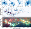 |
Fig. 1 Overview of the entire observed field. The enlarged maps in the first row display several typical hub-filament structures. (a): The background is the integrated intensity map of 13CO (3–2) for the G333 complex, and the boxes show several divided subregions. The letters indicate the substructures studied in this work. The red contours show the peak emission of 13CO (3–2). (b): Overview three-color map of the observed field by combining ATLASGAL+Planck 870 µm (red) and GLIMPSE 8.0 (green) and 4.5 µm (blue) emission, including the G333 complex and GMC G331. |
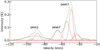 |
Fig. 2 Average spectra of 13CO (3–2) for the entire region. The dashed red profiles represent the components of multi-Gaussian fitting. |
2.2 Archival continuum emission data
The observed region was covered in the infrared by the GLIMPSE survey (Benjamin et al. 2003). The images of the Spitzer Infrared Array Camera (IRAC) at 4.5 and 8.0 µm were retrieved from the Spitzer Archive. The angular resolutions of the images in the IRAC bands are ~ 2″. We also used ATLAS-GAL+Planck 870 µm data (ATLASGAL combined with Planck data), which are sensitive to a wide range of spatial scales at a resolution of ~21″ (Csengeri et al. 2016).
3 Results
3.1 Velocity components
The average emission spectrum of 13CO (3–2) coming from the entire observed field is shown in Fig. 2 together with Gaussian curves used to fit the average spectrum. The fitting was carried out using the GAUSSPY+ software (Riener et al. 2019), which is introduced in detail below. We divided the spectrum into three velocity components [−120, −76] km s−1, [−76, −60] km s−1, and [−60, −35] km s−1 in which emission is prominent. They are labeled peak1, peak2, and peak3. Figure 3 shows that the velocity components peak1 and peak2 represent the main two parts of the G331 GMC, called G331 GMC-blue and G331 GMC-red. Peak3 shows a very extended structure throughout the observed region with the GMC G333 and the G332 ring as the main parts. The four main ATLASGAL clump clusters are labeled A, B, C, and D in Fig. 3a (Urquhart et al. 2018, 2022). They correspond to the different velocity components shown in the moment-one maps of 13CO (3–2) (Fig. 3b). Peak1 and peak2 are associated with clump clusters C and D. Clump clusters A and B are located in velocity component peak3. Peak1 is relatively independent of peak2 and peak3, but the dominant features in peak2 and peak3 appear to overlap to some extent, but they can be separated. Hence, we fit Gaussian functions in order to minimize the effects of cross-contamination. Peak2 and peak3 can be distinguished by the FWHM. We mainly focus on peak3 with the velocity range [−60, −35] km s−1 that represents the complete shell structure shown in Fig. 3e. The association between peak1, peak2, and peak3 will be discussed in detail in a forthcoming paper.
In order to study the structure of the molecular cloud complex in position-position-velocity (PPV) space, we applied the fully automated Gaussian decomposer GAUSSPY+ (Lindner et al. 2015; Riener et al. 2019), which can decompose the complex spectra of molecular lines into multiple Gaussian components. The most important four parameters in the algorithm are the first and second smoothing parameters α1 and α2, the signal-to-noise ratio (S/N) and significance criterion. To determine the smoothing parameters α1 and α2, sets with 500 randomly selected spectra from the 13CO (3–2) cube were used to train GAUSSPY+. The default values of SNR and significance are 3 and 5, but considering that the moment-one map needs a 5σ threshold to show a clear velocity field, we adjusted the value of SNR to 5. The other parameters for the decomposition were set to the default values provided by Riener et al. (2019).
As shown in Fig. 4, the velocity components separated by the average spectrum are consistent with the decomposition of GAUSSPY+. The three main velocity components are well separated in PPV space. Different from peak1 and peak2, peak3 has a large-scale continuous structure, regardless of the projection on Galactic longitude or latitude. This indicates that the structures in peak3 are physically connected. Especially the overall structure of peak3 consists of a large-scale shell structure extended from l = 330.6° to l = 334°. It may be generated by a large-scale compression, such as the shock from supernova explosion events. This will be investigated in a forthcoming paper.
The entire G333 complex seems to have fragmented into several independent molecular clouds. They are treated as subre-gions in Fig. 1, such as s3. The substructures in each subregion marked by letters in Fig. 1a are divided by the bright emission of 13CO (3–2) shown in red contours, such as s3a. Figures 1b and 3a show that the dense parts of the 13CO (3–2) emission tightly correlate with the infrared bright regions. The overlap of different velocity components in subregions 5 and 7 is significant, as shown in Fig. 3a. However, these two subregions only include a few structures in the velocity range [−60, −35] km s−1, thus they are subordinate in the G333 complex.
This analysis shows that the GMC G331 and the G333 complex overlap on the sky, but they have different velocities and lie at very different distances. Because the G333 region is closer to us, we focus the remainder of the paper on it.
3.2 Identification of filaments
The first step was to identify and characterize the filaments in the G333 complex. Following the method described in Zhou et al. (2022), we used the moment-zero maps (the integrated intensity maps) of 13CO (3–2) to identify filaments in the G333 complex using the FILFINDER algorithm (Koch & Rosolowsky 2015). The velocity intervals for making moment-zero maps were determined from the averaged spectra of each subregion. They are marked by the vertical dotted lines in Fig. A.1. Moreover, a threshold of 5σ was applied to make the moment maps, which can reduce the noise contamination effectively. The skeletons of identified filaments overlaid on the moment-zero maps of the13 CO (3–2) line emission are shown in Fig. 5. They are highly consistent with the gas structures traced by 13CO (3–2) as seen by eye, indicating that the structures identified in FILFINDER are reliable. Then for each subregion, we broke the filamentary network into several filaments. This step is necessary to calculate the offset along the filament before fitting the velocity gradient. To show the velocity field along the filament more clearly, we tried to make each filament long enough.
Because each subregion includes many substructures, it is not surprising that their average spectra will show multiple velocity peaks. In Fig. A.1, the average spectra of G333-s3 clearly show multiple components. We separated each peak in the line profile and found that each peak indeed corresponded to a substructure. This situation may also exist in other subregions. However, these sub-structures are generally well separated spatially and thus have no significant impact on the moment-map analysis.
Figure 6 displays the GAUSSPY+ decomposition of each subregion in PPV space. It shows that the main structures of each subregion are connected in PPV space and thus are unlikely to be contaminated by velocity components from unrelated foreground or background cloud emission. Moreover, after we extracted the velocity and intensity information along the filament skeletons, we should find anomalies in Fig. 7 if unrelated velocity components overlap. The anomalies might be a sudden break at a certain position of the skeleton. However, this is not the case in our analysis. Furthermore, we only analyze the variations of velocity and intensity along the filament skeletons with a width of one pixel, which can also effectively avoid potential overlap. In Zhou et al. (2022), we found that multiple velocity components are common in hub-filament systems, especially in hub regions. Furthermore, the observed samples in Zhou et al. (2022) with or without multiple velocity components show similar results, such as the velocity gradient estimated from the moment maps.
We can assume that most of the pixels above the filaments have a single velocity component or have a dominant velocity component. When we compare the fitting results with the freefall model and previous results from ALMA data, the hypothesis is indicated as reasonable if the results are consistent. This is the case in our work. Conversely, if the overlap of velocity components is significant, the fitted velocity gradient should be free without the regularities shown in our work because the overlap of unrelated velocity components is random. Figure 7 shows good correlations between velocity and density fluctuations, which is consistent with previous studies (Hacar & Tafalla 2011; Henshaw et al. 2014, 2016, 2020; Liu et al. 2019). The variation in the velocity gradient with the scale shown in Fig. 8 is also consistent with the results in Zhou et al. (2022).
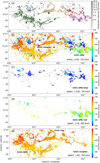 |
Fig. 3 ATLASGAL clump distribution and velocity components of the entire observed field. (a): The background is the integrated intensity map of 13CO (3–2). The color-coded plus indicates the different ATLASGAL clump clusters A (green), B (orange), C (red), and D (magenta). (b): The moment-one map of 13CO (3–2) for the entire region in the overall velocity range. Panels c–e: Moment-one map of 13CO (3–2) for the three peaks marked in Fig. 2. |
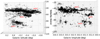 |
Fig. 4 Velocity distribution of the entire observed field in PPV space decomposed by GAUSSPY+ along the Galactic latitude and longitude. |
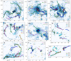 |
Fig. 5 Background images showing the moment-zero maps of 13CO (3–2). The lines in color present the filament skeletons. The orange circles show the ATLASGAL clumps. The size of the circle represents the clump radius. The red plus marks the intensity peak of 13CO (3–2) emission in Fig. 7. |
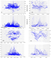 |
Fig. 6 Intensity and velocity distribution of the subregions in PPV space based on the decomposition of GAUSSPY+. For other subregions, see Figs. A.2 and A.3. |
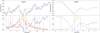 |
Fig. 7 Two selected filaments illustrate the fitting of the velocity gradient. Upper panels: velocity gradients are fit in the ranges defined by the vertical dashed red lines, and straight lines show the linear fitting results. Lower panels: dotted blue and red lines show the normalized velocity and intensity, respectively. The orange circles mark the intensity peaks of 13CO (3–2) emission associated with ATLASGAL clumps. For other filaments, see Figs. A.4–A.8. |
3.3 Velocity gradients
The kinematical features of hub-filament systems can be revealed by the velocity gradients along the filaments. However, it is difficult to directly carry out the measurement in PPV space due to the complex gas motion shown in Fig. 4. In Zhou et al. (2022), we investigated hub-filament systems in a large sample of 146 protoclusters using the H13CO+ J = 1–0 molecular line in the ATOMS survey. The strongest intensity peaks of the H13CO+ emission coincide with the brightest 3 mm cores or hub regions in these hub-filament systems. We find that filaments are ubiquitous in protoclusters. Velocity and density fluctuations along these filaments are seen. We first estimated two overall velocity gradients between the velocity peaks and valleys at the two sides of the center of the gravitational potential well and ignored local velocity fluctuation. We also derived additional velocity gradients over smaller distances around the strongest intensity peaks of the H13CO+ emission (see Fig. 6 in Zhou et al. 2022). In this work, the same method was used to derive the velocity gradients from the LAsMA data. Then the fitted velocity gradients derived from the LAsMA and ALMA data were combined for a statistical analysis, as shown in Fig. 8.
Figure 7 shows the intensity-weighted velocity (moment-one) and integrated intensity (moment-zero) map of the 13CO (3–2) line emission along the skeletons of selected filaments with intense velocity and density fluctuations along these filaments. Generally, the peaks of the density fluctuations are associated with ATLASGAL clumps, as shown in Fig. 5. The density and velocity fluctuations along the filaments may indicate converging gas flows coupled to regularly spaced density enhancements that probably form via gravitational instabilities (Henshaw et al. 2020). Figure 7 shows the typical V-shape velocity structure around the intensity peaks, which we fit as velocity gradients on either side of the intensity peak marked by the straight lines. Figure 7a shows a more complex velocity field with more repetitive segments than the simple structure in Fig. 7b. The gas kinematics of other long filaments in Fig. 5 are similar to those in Fig. 7a. For the long filaments, except for the local velocity fluctuations or gradients, they also exhibit velocity gradients on larger scales, which were fit by ignoring the local velocity fluctuations. Generally, large-scale velocity gradients are associated with several intensity peaks.
3.4 Hub-filament structure
Each subregion marked in Fig. 1a contains many substructures that are nearly separated from each other, except for several crowded regions. The red contours from ~50% of the integrated intensity of the 13CO (3–2) emission show the high-density parts of various structures. In Fig. 1, several typical hub-filament structures are highlighted in the first row; see also Fig. 5 for more details. The filamentary structures are connected to high-density hubs. Other substructures in the entire observed region have a more or less similar morphology. Some differences are expected because the appearance of the hub-filament morphology relies on the projection angle and on the resolution of the observation. Moreover, most structures have the typical kinematic features of hub-filament systems, as discussed in the next sections. For example, the intensity peaks (the hubs) are associated with the converging velocities, indicating that the surrounding gas flows may be converging to dense structures. In particular, the velocity gradients increase at small scales.
The orange circle in Fig. 7 marks the intensity peak of 13CO (3– 2) emission associated with an ATLASGAL clump. The distance between the central coordinate of the ATLASGAL clump and the intensity peak of the 13CO (3–2) emission is smaller than the effective radius of the ATLASGAL clump. These associated clumps are treated as hubs in this work. Their properties are listed in Tables 1 and 2. In Table 2, some of the peaks have more than one corresponding ATLASGAL clump, and we have added these together, as indicated by a space in the table. We focus on their mass, effective radius, and the corresponding velocity gradients. However, as shown in Fig. 7, many peaks of the 13CO (3–2) emission lack corresponding clumps. They were therefore not included in the tables, but are similar to the peaks associated with clumps. Generally, the large-scale velocity gradients involve many intensity peaks with or without corresponding clumps. It is therefore difficult to estimate the properties of their hubs, and therefore, these are not given in the tables.
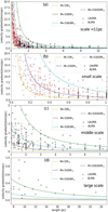 |
Fig. 8 Statistical analysis of all fitted velocity gradients. (a): Velocity gradient vs. the length over which the gradient has been estimated for all sources in the ATOMS survey (red dots) and current LAsMA observation (black plus). The color lines show the freefall velocity gradients for comparison. For the freefall model, yellow, blue, cyan, and green lines denote masses of 5 M⊙, 500 M⊙, 5000 M⊙, and 50 000 M⊙, respectively. Panels b–d: zoomed maps with lengths <1 pc (small scale), ~ 1–7.5 pc (medium scale), and >7.5 pc (large scale) in panel a. |
3.5 Funnel structure
When we compare the velocity gradients of the molecular gas to iron filings, the distribution of the velocity gradients may to some extent reflect the shape of the force field that plays the dominant role in the molecular clouds, just as the iron filings can reflect the shape of a magnetic field. Below, we investigate the distribution of the molecular velocity gradients in PPV space. In the case of gravitational freefall onto a central point mass, velocities change as  . In the case of a collapse that is driven by the gravity of a gaseous mass with a certain density profile, the radial dependence of the infall speed depends on the slope of the density profile (Gómez et al. 2021). In either case, this results in a funnel morphology of the velocity field in PPV space, as illustrated in Fig. 9. The exterior cloud velocities show only gentle variations (a small velocity gradient that funnels material from the cloud to the clump), while the velocities in the interior part near the center change dramatically with scales (a large velocity gradient that funnels material from the clump to the core). We note that the schematic in Fig. 9 is oversimplified. A molecular cloud generally contains many clumps, and a clump also contains many cores. We chose only one clump and one core to demonstrate the gas inflow and the variation in the velocity gradient from the molecular cloud scale to the core scale. A more realistic case is shown in Fig. 6, where most of the substructures indeed show the expected funnel structures in PPV space. Particularly close to the intensity peak, the velocity gradient increases steeply, as also reflected in Fig. 7.
Moreover, the V-shape velocity structure around the intensity peaks indicates accelerated material inflowing toward the central hub (Gómez & Vázquez-Semadeni 2014; Kuznetsova et al. 2015, 2018; Hacar et al. 2017; Zhou et al. 2022), which is shown everywhere in Fig. 7. The V-shape velocity structure can be treated as the projection of the funnel structure from PPV space to the PV plane. Hence, the funnel structures in PPV space can be an effective probe for the gravitational collapse motions in molecular cloud.
4 Discussion
4.1 Characteristic scale ~ 1 pc
We have investigated gas motions on sufficiently large scales. The longest filament was ~50 pc. We obtained results similar to previous small-scale ALMA observations. We fit a wide range of values of the velocity gradients, as shown in Fig. 8a. The velocity gradients are small at large scales, while they become significantly larger at small scales (≲ 1 pc), as is the case in the ATOMS survey (Zhou et al. 2022). For both ALMA and LAsMA data, most of the fit velocity gradients are concentrated on the scales ~1 pc, as shown in Fig. 8. This is consistent with the fact that 1 pc is considered the characteristic scale of massive clumps (Urquhart et al. 2018). In Fig. 8 the variation in the velocity gradients with the scales is comparable with the expectations from gravitational freefall, in the sense that the gradient decreases smoothly with increasing scale. Figures 10c,d show results similar to those in Fig. 8, but only consider the velocity gradients associated with ATLASGAL clumps that are listed in Tables 1 and 2. In particular, in Fig. 10c, the required central mass in the fitted freefall model is consistent with the mass distribution observed in Fig. 10b.
4.2 Evidence for gravitational acceleration
Figure 10a displays the probability distribution of velocity gradients measured around 1 pc (0.8 ~ 1.2 pc), showing that the most frequent velocity gradient is ~1.6 km s−1 pc−1. Assuming freefall,
 (1)
(1)
we estimate that the kinematic mass corresponding to 1 pc is ~1190 M⊙, which is comparable with the typical mass of clumps in the ATLASGAL survey (Urquhart et al. 2018). In Fig. 10b, the peak of the associated clump mass distribution is also ~1000 M⊙. Thus the clump may be a gravity-dominated collapsing object, which is also consistent with the survey results that most Galactic parsec-scale massive clumps seem to be gravitationally bound, regardless of how evolved they are (Liu et al. 2016a; Urquhart et al. 2018; Evans et al. 2021).
Based on Eq. (1), we can use the values of M, L, and ∇V listed in Tables 1 and 2 to compare the observations to the simple theory. In Fig. 11 the observed and predicted accelerations are clearly correlated. This is strong evidence that gravity accelerates the gas inflow. The scatter in Fig. 11 is to be expected because we measured only the projection of the realistic velocity vector and hence acceleration. For the same reason, we tend to underestimate the observed acceleration. Moreover, in Tables 1 and 2, we only selected the ATLASGAL clumps associated with the intensity peaks of the 13CO (3–2) emission (a deviation within the effective radius of the clump), thus some of them are not the exact gravitational centers. Despite these caveats, the correlation between observations and predictions for the denser clumps is quite good. The less dense clumps tend to lie above the line of equality, suggesting that their masses underestimate the total mass contributing to the gravitational acceleration.
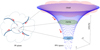 |
Fig. 9 Schematic diagram of the funnel structure in PPV space and on the PP plane. The PP plane shows the multiscale hub−filament structure in a molecular cloud, which can turn into a funnel structure in PPV space. The red arrow represents the gas inflow. |
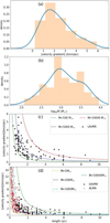 |
Fig. 10 Statistical analysis of the velocity gradients listed in Table 1. (a): Probability distribution of the velocity gradients measured around the 1 pc scale, (b): Mass distribution of ATLASGAL clumps listed in Tables 1 and 2. Panels c and d: same as Fig. 8, but only for the velocity gradients listed in Tables 1 and 2. |
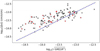 |
Fig. 11 Correlation between the left and right terms in Eq. (1) revealed by the values of M, L, and ∇V listed in Tables 1 and 2. The dotted blue line is the line of equality of the left and right terms. Tables 1 and show two cases. A dense clump with two or more filaments leading to it, or only one filament with a gradient that can be identified (the rows with only one entry for the gradient). The number of clumps in the two cases is 49 and 25, and they marked by black and red plus, respectively. |
4.3 Large-scale inflow driven by gravity
As shown in Figs. 8 and 10, the velocity gradients we fit to the LAsMA and ALMA data agree with each other over the range of scales covered by ALMA observations in the ATOMS survey (<5 pc). Interestingly, the variations in velocity gradients at small scales (< 1 pc), medium scales (~ 1–7.5 pc), and large scales (>7.5 pc) are consistent with gravitational freefall with central masses of ~500 M⊙, ~5000 M⊙, and ~50 000 M⊙. This means that the velocity gradients on larger scales require a higher mass to be maintained, which is also revealed by the funnel structure shown in Fig. 9. Higher masses imply larger scales, that is to say, the larger-scale inflow is driven by the larger-scale structure, which may be the gravitational clustering of smaller-scale structures (Sect. 4.4), consistent with the hierarchical structure in molecular clouds and the gas inflow from large to small scales. Thus the large-scale gas inflow may also be driven by gravity, with the molecular clouds in G333 in a state of global gravitational collapse, which is consistent with the argument that these molecular clouds act as cloud-scale hub-filament structures (see the description in Sect. 3.4). Moreover, as described in Sect. 3.5, the funnel structure of the velocity field shown in PPV space also tends to support the large-scale gravitational collapse of the molecular clouds in the G333 complex.
4.4 Hierarchical gravitational structure in the molecular cloud
The scales of the hub-filament structures (cloud-scale) in this work are much larger than those (clump-scale) in Zhou et al. (2022). Each large-scale hub-filament structure will contain many sub-structures, and the kinematic structure will therefore be very complex. Nevertheless, if they are hub-filament systems, we expect that they have similar kinematic features as the clump-scale hub-filament system. A hub-filament system must have a common gravitational center, which will dominate the overall gravitational field and thus the velocity field. Although Fig. 4 shows many substructures in each subregion, which cause many velocity and density fluctuations, the entire large-scale structure globally still displays the funnel structure. As discussed in Sects. 3.3 and 4.3, large-scale velocity gradients always involve many intensity peaks, and the larger-scale inflow is driven by the larger-scale structure, implying that the clustering of local small-scale gravitational structures can act as the gravitational center on a larger scale. To some extent, the funnel structure gives an indication of the gravitational potential well that is formed by the clustering.
Both Zhou et al. (2022) and this work find that when the scale is smaller than ~1 pc, the gravitationally dominated gas infall can become apparent. Thus, relatively small-scale hub-filament structures will have better and more recognizable morphology than large-scale ones due to the strong local gravitational field. For the large-scale hub-filament structures, background turbulence is more likely to disturb their morphology due to weaker gravitational confinement on large scales, thus they are more strongly blurred. Zhou et al. (2023) suggested for the interpretation of the formation of the large-scale hub-filament structure in W33 complex that IRDCs and ATLASGAL clumps in W33-blue can be treated as small-scale hub-filament structures, and W33-blue itself as a huge hub-filament structure. This means that there may be a self-organization process from small-scale hub-filament structures to a large-scale one. If the large-scale gravitational center is the clustering of small-scale ones, the large-scale gravity center will be more loose compared to the latter. Its ability to control the gas motions on a large scale is therefore also weaker, which is reflected as the loose funnel structure and small velocity gradient, as shown in this work. In Fig. 6 the small-scale structures indeed have clearer funnel structures than the large-scale ones. This indicates the role of gravity in shaping the funnel structure.
4.5 G333 in the context of Galactic molecular clouds
The same region of the sky, with a slightly larger area (332.6° < l < 333.8° and −0.8° < b < 0.1°), was also studied by Nguyen et al. (2015) using CO and 13CO (1–0) emission and archival data. They called the GMC G333 the RCW 106 complex after the associated H II region. They determined the following properties for the RCW 106 complex: the total effective diameter is 183 pc, the mass is 5.9 × 10⁶ M⊙, and the mass surface density is 220 M⊙ pc−2. The virial parameter for the whole complex is 0.35, making it strongly gravitationally bound. Because the cloud is elongated, they included a linear analysis that also implied a strongly bound cloud. These properties would mean that the GMC G333 iss one of the largest most massive complexes in the Galaxy (see Fig. 7 of Miville-Deschênes et al. 2017), and one of the few that is gravitationally bound (see Fig. 2 of Evans et al. 2021). However, Nguyen et al. (2015) took the velocity range of the RCW 106 complex as [−80, −40] km s−1. As discussed in Sect. 3.1, after decomposing the velocity components, we find that the velocity range [−80, −40] km s−1 also includes the GMC G331. The mass of the GMC G333 is therefore overestimated in Nguyen et al. (2015). The catalog of Miville-Deschênes et al. (2017), restricted to the velocity range of peak3, yields a mass for the G333 cloud traced by CO 1–0 emission of ~1.7 × 10⁶ M⊙, with the surface density ~120 M⊙ pc−2. Tracers that are biased toward higher volume densities find progressively lower masses. Karnik et al. (2001) made a far-infrared (FIR) 150 and 210 µm dust emission study of the region using the canonical gas-to-dust ratio of 100. They measured a total GMC mass of ~1.8 × 10⁵ M⊙. This is consistent with the total mass of ~1 × 10⁵ M⊙ estimated by Mookerjea et al. (2004) from a 1.2 mm cold dust continuum emission map and the same gas-to-dust ratio. These estimates show the decreasing fraction of mass in progressively denser regions.
The lower total mass from CO 1–0 based on the catalog of Miville-Deschênes et al. (2017) still makes the G333 complex one of the most massive in the Milky Way. The analysis of the RCW HII region yields a stellar mass of 48 × 103 M⊙. Assuming a timescale of 0.2 Myr (for an O7 star starting from its first appearance on the main-sequence diagram), Nguyen et al. (2015) derived a star formation rate so far of 0.25 M⊙ Myr−1 and an efficiency (M*/Mgas) of 0.008. The very high star formation rate led Nguyen et al. (2015) to describe it as a mini-starburst. It is thus atypical of most molecular clouds, but an exemplar of the very small subset that forms the majority of stars in the Galaxy.
5 Summary
We investigated the gas kinematics of hub-filament structures in the G333 complex using 13CO (3–2) emission. The main conclusions are listed below.
The G333 complex includes three main velocity components, which can be well separated by the average spectra and the velocity distribution in PPV space. We derived the velocity distribution from the decomposition of 13CO (3–2) emission by GAUSSPY+. The velocity components with velocity ranges [−120, −76] km s−1 and [−76, −60] km s−1 represent the main two parts of GMC G331. The third velocity component with the velocity range [−60, −35] km s−1 shows a very extended shell structure from l = 330.6° to l = 334° with GMC G333 and the G332 ring as the main parts.
The entire G333 complex seems to have fragmented into several independent molecular clouds. Some of the substructures in these molecular clouds show typical hub-filament structures, which also have the typical kinematic features of hub-filament systems. The broken morphology of some very infrared bright structures indicates that the feedback is disrupting the star-forming regions.
We used the integrated intensity maps of 13CO J = 3–2 to identify filaments in the G333 complex by FILFINDER algorithm and extracted the velocity and intensity along the filament skeleton from moment maps. We find a good correlation between velocity and density fluctuations, and we fit the velocity gradients around the intensity peaks. The change in velocity gradients with the scale indicates that the morphology of the velocity field in PPV space resembles a funnel structure. The funnel structure can be explained as accelerated material inflowing toward the central hub and gravitational contraction of star-forming clouds or clumps. The typical V-shape velocity structure along the filament skeleton can be treated as the projection of the funnel structure from PPV space onto the PV plane. Hence, the funnel structure in PPV space can be an effective probe for the gravitational collapse motion in molecular cloud.
We investigated gas motions on sufficiently large scales. The longest filament was ~50 pc. We obtained results similar to small-scale ALMA observations, however. The typical velocity gradient corresponding to a one-parsec scale is ~ 1.6 km s−1 pc−1. Assuming the freefall model, we can predict the gravitational acceleration onto each hub. The observed accelerations correlate well with the predicted ones and the values arecomparable to the prediction. Because we observe only one component of the acceleration and because the masses of the hubs are uncertain, the result provides strong evidence for gravitational acceleration of material flowing into hubs from filaments.
The velocity gradients fit with LAsMA data and ALMA data agree with each other over the scales covered by ALMA observations in the ATOMS survey (<5 pc). On large scales, we find that the larger-scale inflow is driven by the larger-scale structure, indicating the hierarchical structure in the molecular cloud and the gas inflow from large scale to small scale. The large-scale gas inflow is driven by gravity, implying that the molecular clouds in G333 may be in a state of global gravitational collapse. The funnel structure of the velocity field shown in PPV space also tends to support the large-scale gravitational collapse.
Although there are many substructures in each molecular cloud that cause ubiquitous velocity and density fluctuations, the entire large-scale structure in total still displays a loose funnel structure. Thus the hub-filament structures at different scales may be organized into a hierarchical macroscopic system through the coupling of gravitational centers at different scales.
In short, the changes in velocity gradient with scale indicate a funnel structure of the velocity field in PPV space. This is indicative of a smooth, continuously increasing velocity gradient from large to small scales, and it is thus consistent with gravitational acceleration.
Acknowledgements
This publication is based on data acquired with the Atacama Pathfinder Experiment (APEX) under programme ID M-0109.F-9514A-2022. APEX has been a collaboration between the Max-Planck-Institut für Radioastronomie, the European Southern Observatory, and the Onsala Space Observatory. This work has been supported by the National Key R&D Program of China (No. 2022YFA1603100). T.L. acknowledges the supports by National Natural Science Foundation of China (NSFC) through grants No.12122307 and No.12073061, the international partnership program of Chinese Academy of Sciences through grant No.114231KYSB20200009, and Shanghai Pujiang Program 20PJ1415500.
Appendix A Supplementary maps
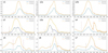 |
Fig. A.1 Average spectra of 13CO (3–2) and 12CO (3–2) for the subregions shown in Fig.5. The vertical dashed lines mark the velocity ranges that are used to make the moment maps. |
Appendix B Appendix A: Noise and offset details
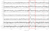 |
Fig. B.1 Average spectra in one beam size of 7 pixels for the off-position. |
The receiver is a hexagonal array of six pixels surrounding a central pixel. The outer array is separated from the central pixel by ~ 2 FWHM. Table. B.1 lists the offsets of the outer 6 pixels relative to the central pixel. Fig. B.1 shows the average spectra in one beam size of 7 pixels for the off-position. The emission is mainly concentrated in the velocity range [−50,−15] km s−1. The absorption feature of one submap shown in Fig. B.3 also appears in the same velocity range. We therefore added the emission of the off-position in the velocity range [−50,−15] km s−1 to each submap. As shown in Fig. B.3, the absorption feature indeed disappears after the emission of the off-position is added.
Offsets of the outer 6 pixels relative to the central pixel.
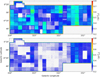 |
Fig. B.2 Noise maps of 13CO (3–2) and 12CO (3–2) in our observation. |
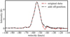 |
Fig. B.3 Average spectra of one submap G333D55M-7M. |
References
- Bains, I., Wong, T., Cunningham, M., et al. 2006, MNRAS, 367, 1609 [NASA ADS] [CrossRef] [Google Scholar]
- Ballesteros-Paredes, J., Hartmann, L. W., Vázquez-Semadeni, E., Heitsch, F., & Zamora-Avilés, M. A. 2011, MNRAS, 411, 65 [NASA ADS] [CrossRef] [Google Scholar]
- Benjamin, R. A., Churchwell, E., Babler, B. L., et al. 2003, PASP, 115, 953 [Google Scholar]
- Bonnell, I. A., Bate, M. R., Clarke, C. J., & Pringle, J. E. 1997, MNRAS, 285, 201 [NASA ADS] [CrossRef] [Google Scholar]
- Bonnell, I. A., Bate, M. R., Clarke, C. J., & Pringle, J. E. 2001, MNRAS, 323, 785 [Google Scholar]
- Breen, S. L., Ellingsen, S. P., Johnston-Hollitt, M., et al. 2007, MNRAS, 377, 491 [NASA ADS] [CrossRef] [Google Scholar]
- Breen, S. L., Ellingsen, S. P., Caswell, J. L., et al. 2012, MNRAS, 421, 1703 [NASA ADS] [CrossRef] [Google Scholar]
- Bronfman, L., Alvarez, H., Cohen, R. S., & Thaddeus, P. 1989, ApJS, 71, 481 [NASA ADS] [CrossRef] [Google Scholar]
- Caswell, J. L. 1998, MNRAS, 297, 215 [NASA ADS] [CrossRef] [Google Scholar]
- Caswell, J. L., & Haynes, R. F. 1987, A&A, 171, 261 [NASA ADS] [Google Scholar]
- Caswell, J. L., Haynes, R. F., & Goss, W. M. 1980, Australian J. Phys., 33, 639 [NASA ADS] [CrossRef] [Google Scholar]
- Caswell, J. L., Vaile, R. A., & Forster, J. R. 1995, MNRAS, 277, 210 [NASA ADS] [Google Scholar]
- Caswell, J. L., Fuller, G. A., Green, J. A., et al. 2011, MNRAS, 417, 1964 [Google Scholar]
- Chen, H.-R. V., Zhang, Q., Wright, M. C. H., et al. 2019, ApJ, 875, 24 [Google Scholar]
- Chen, M. C.-Y., Di Francesco, J., Rosolowsky, E., et al. 2020, ApJ, 891, 84 [NASA ADS] [CrossRef] [Google Scholar]
- Clarke, S. D., Whitworth, A. P., & Hubber, D. A. 2016, MNRAS, 458, 319 [CrossRef] [Google Scholar]
- Csengeri, T., Weiss, A., Wyrowski, F., et al. 2016, A&A, 585, A104 [NASA ADS] [CrossRef] [EDP Sciences] [Google Scholar]
- Cunningham, M., Lo, N., Kramer, C., et al. 2008, EAS Publ. Ser., 31, 9 [NASA ADS] [CrossRef] [EDP Sciences] [Google Scholar]
- Dewangan, L. K., Ojha, D. K., Sharma, S., et al. 2020, ApJ, 903, 13 [Google Scholar]
- Elmegreen, B. G., Elmegreen, D. M., & Efremov, Y. N. 2018, ApJ, 863, 59 [NASA ADS] [CrossRef] [Google Scholar]
- Evans, N. J., II, Heyer, M., Miville-Deschênes, M.-A., Nguyen-Luong, Q., & Merello, M. 2021, ApJ, 920, 126 [NASA ADS] [CrossRef] [Google Scholar]
- Fujiyoshi, T., Smith, C. H., Caswell, J. L., et al. 2006, MNRAS, 368, 1843 [NASA ADS] [CrossRef] [Google Scholar]
- Gómez, G. C., & Vázquez-Semadeni, E. 2014, ApJ, 791, 124 [Google Scholar]
- Gómez, G. C., Vázquez-Semadeni, E., & Palau, A. 2021, MNRAS, 502, 4963 [CrossRef] [Google Scholar]
- Goss, W. M., Manchester, R. N., & Robinson, B. J. 1970, Australian J. Phys., 23, 559 [Google Scholar]
- Güsten, R., Nyman, L. Å., Schilke, P., et al. 2006, A&A, 454, L13 [NASA ADS] [CrossRef] [EDP Sciences] [Google Scholar]
- Hacar, A., & Tafalla, M. 2011, A&A, 533, A34 [NASA ADS] [CrossRef] [EDP Sciences] [Google Scholar]
- Hacar, A., Alves, J., Tafalla, M., & Goicoechea, J. R. 2017, A&A, 602, L2 [NASA ADS] [CrossRef] [EDP Sciences] [Google Scholar]
- Hartmann, L., Ballesteros-Paredes, J., & Heitsch, F. 2012, MNRAS, 420, 1457 [Google Scholar]
- Henshaw, J. D., Caselli, P., Fontani, F., Jiménez-Serra, I., & Tan, J. C. 2014, MNRAS, 440, 2860 [Google Scholar]
- Henshaw, J. D., Longmore, S. N., & Kruijssen, J. M. D. 2016, MNRAS, 463, L122 [NASA ADS] [CrossRef] [Google Scholar]
- Henshaw, J. D., Kruijssen, J. M. D., Longmore, S. N., et al. 2020, Nat. Astron., 4, 1064 [CrossRef] [Google Scholar]
- Issac, N., Tej, A., Liu, T., et al. 2019, MNRAS, 485, 1775 [NASA ADS] [CrossRef] [Google Scholar]
- Jordan, C. H., Walsh, A. J., Lowe, V., et al. 2013, MNRAS, 429, 469 [NASA ADS] [CrossRef] [Google Scholar]
- Karnik, A. D., Ghosh, S. K., Rengarajan, T. N., & Verma, R. P. 2001, MNRAS, 326, 293 [NASA ADS] [CrossRef] [Google Scholar]
- Kirk, H., Myers, P. C., Bourke, T. L., et al. 2013, ApJ, 766, 115 [Google Scholar]
- Koch, E. W., & Rosolowsky, E. W. 2015, MNRAS, 452, 3435 [Google Scholar]
- Krumholz, M. R., Klein, R. I., & McKee, C. F. 2007, ApJ, 656, 959 [NASA ADS] [CrossRef] [Google Scholar]
- Kuznetsova, A., Hartmann, L., & Ballesteros-Paredes, J. 2015, ApJ, 815, 27 [NASA ADS] [CrossRef] [Google Scholar]
- Kuznetsova, A., Hartmann, L., & Ballesteros-Paredes, J. 2018, MNRAS, 473, 2372 [NASA ADS] [CrossRef] [Google Scholar]
- Lindner, R. R., Vera-Ciro, C., Murray, C. E., et al. 2015, AJ, 149, 138 [NASA ADS] [CrossRef] [Google Scholar]
- Liu, T., Kim, K.-T., Yoo, H., et al. 2016a, ApJ, 829, 59 [NASA ADS] [CrossRef] [Google Scholar]
- Liu, T., Zhang, Q., Kim, K.-T., et al. 2016b, ApJ, 824, 31 [Google Scholar]
- Liu, H.-L., Stutz, A., & Yuan, J.-H. 2019, MNRAS, 487, 1259 [Google Scholar]
- Liu, T., Evans, N. J., Kim, K.-T., et al. 2020, MNRAS, 496, 2790 [Google Scholar]
- Liu, H.-L., Tej, A., Liu, T., et al. 2022, MNRAS, 511, 4480 [NASA ADS] [CrossRef] [Google Scholar]
- Lo, N., Cunningham, M. R., Jones, P. A., et al. 2009, MNRAS, 395, 1021 [NASA ADS] [CrossRef] [Google Scholar]
- Lockman, F. J. 1979, ApJ, 232, 761 [NASA ADS] [CrossRef] [Google Scholar]
- Lowe, V., Cunningham, M. R., Urquhart, J. S., et al. 2014, MNRAS, 441, 256 [NASA ADS] [CrossRef] [Google Scholar]
- Lu, X., Zhang, Q., Liu, H. B., et al. 2018, ApJ, 855, 9 [Google Scholar]
- Mazumdar, P., Wyrowski, F., Colombo, D., et al. 2021, A&A, 650, A164 [NASA ADS] [CrossRef] [EDP Sciences] [Google Scholar]
- McKee, C. F., & Ostriker, E. C. 2007, ARA&A, 45, 565 [Google Scholar]
- McKee, C. F., & Tan, J. C. 2003, ApJ, 585, 850 [Google Scholar]
- Merello, M., Bronfman, L., Garay, G., et al. 2013, ApJ, 774, 38 [NASA ADS] [CrossRef] [Google Scholar]
- Misugi, Y., Inutsuka, S.-I., & Arzoumanian, D. 2019, ApJ, 881, 11 [NASA ADS] [CrossRef] [Google Scholar]
- Miville-Deschênes, M.-A., Murray, N., & Lee, E. J. 2017, ApJ, 834, 57 [Google Scholar]
- Mookerjea, B., Kramer, C., Nielbock, M., & Nyman, L. Å. 2004, A&A, 426, 119 [NASA ADS] [CrossRef] [EDP Sciences] [Google Scholar]
- Motte, F., Bontemps, S., & Louvet, F. 2018, ARA&A, 56, 41 [NASA ADS] [CrossRef] [Google Scholar]
- Nguyen, H., Nguyen Lu’o’ng, Q., Martin, P. G., et al. 2015, ApJ, 812, 7 [NASA ADS] [CrossRef] [Google Scholar]
- Padoan, P., Pan, L., Juvela, M., Haugbølle, T., & Nordlund, Å. 2020, ApJ, 900, 82 [NASA ADS] [CrossRef] [Google Scholar]
- Peretto, N., Fuller, G. A., Duarte-Cabral, A., et al. 2013, A&A, 555, A112 [NASA ADS] [CrossRef] [EDP Sciences] [Google Scholar]
- Pestalozzi, M. R., Minier, V., & Booth, R. S. 2005, A&A, 432, 737 [NASA ADS] [CrossRef] [EDP Sciences] [Google Scholar]
- Pillai, T. G. S., Clemens, D. P., Reissl, S., et al. 2020, Nat. Astron., 4, 1195 [Google Scholar]
- Riener, M., Kainulainen, J., Henshaw, J. D., et al. 2019, A&A, 628, A78 [NASA ADS] [CrossRef] [EDP Sciences] [Google Scholar]
- Romano, D., Burton, M. G., Ashley, M. C. B., et al. 2019, MNRAS, 484, 2089 [NASA ADS] [CrossRef] [Google Scholar]
- Russeil, D. 2003, A&A, 397, 133 [CrossRef] [EDP Sciences] [Google Scholar]
- Russeil, D., Adami, C., Amram, P., et al. 2005, A&A, 429, 497 [NASA ADS] [CrossRef] [EDP Sciences] [Google Scholar]
- Smith, R. J., Glover, S. C. O., Klessen, R. S., & Fuller, G. A. 2016, MNRAS, 455, 3640 [Google Scholar]
- Ulich, B. L., & Haas, R. W. 1976, ApJS, 30, 247 [Google Scholar]
- Urquhart, J. S., König, C., Giannetti, A., et al. 2018, MNRAS, 473, 1059 [Google Scholar]
- Urquhart, J. S., Wells, M. R. A., Pillai, T., et al. 2022, MNRAS, 510, 3389 [NASA ADS] [CrossRef] [Google Scholar]
- Vallée, J. P. 2008, AJ, 135, 1301 [CrossRef] [Google Scholar]
- Vázquez-Semadeni, E., Gómez, G. C., Jappsen, A. K., Ballesteros-Paredes, J., & Klessen, R. S. 2009, ApJ, 707, 1023 [CrossRef] [Google Scholar]
- Vázquez-Semadeni, E., González-Samaniego, A., & Colín, P. 2017, MNRAS, 467, 1313 [NASA ADS] [Google Scholar]
- Vázquez-Semadeni, E., Palau, A., Ballesteros-Paredes, J., Gómez, G. C., & Zamora-Avilés, M. 2019, MNRAS, 490, 3061 [Google Scholar]
- Wang, P., Li, Z.-Y., Abel, T., & Nakamura, F. 2010, ApJ, 709, 27 [NASA ADS] [CrossRef] [Google Scholar]
- Williams, G. M., Peretto, N., Avison, A., Duarte-Cabral, A., & Fuller, G. A. 2018, A&A, 613, A11 [NASA ADS] [CrossRef] [EDP Sciences] [Google Scholar]
- Wong, T., Ladd, E. F., Brisbin, D., et al. 2008, MNRAS, 386, 1069 [NASA ADS] [CrossRef] [Google Scholar]
- Yuan, J., Li, J.-Z., Wu, Y., et al. 2018, ApJ, 852, 12 [Google Scholar]
- Zhang, Q., Wang, K., Lu, X., & Jiménez-Serra, I. 2015, ApJ, 804, 141 [Google Scholar]
- Zhou, J.-W., Liu, T., Evans, N. J., et al. 2022, MNRAS, 514, 6038 [NASA ADS] [CrossRef] [Google Scholar]
- Zhou, J.-W., Li, S., Liu, H.-L., et al. 2023, MNRAS, 519, 2391 [Google Scholar]
This publication is based on data acquired with the Atacama Pathfinder Experiment (APEX). APEX is a collaboration between the Max-Planck-Institut für Radioastronomie, the European Southern Observatory and the Onsala Space Observatory.
All Tables
All Figures
|
Fig. 1 Overview of the entire observed field. The enlarged maps in the first row display several typical hub-filament structures. (a): The background is the integrated intensity map of 13CO (3–2) for the G333 complex, and the boxes show several divided subregions. The letters indicate the substructures studied in this work. The red contours show the peak emission of 13CO (3–2). (b): Overview three-color map of the observed field by combining ATLASGAL+Planck 870 µm (red) and GLIMPSE 8.0 (green) and 4.5 µm (blue) emission, including the G333 complex and GMC G331. |
| In the text | |
|
Fig. 2 Average spectra of 13CO (3–2) for the entire region. The dashed red profiles represent the components of multi-Gaussian fitting. |
| In the text | |
|
Fig. 3 ATLASGAL clump distribution and velocity components of the entire observed field. (a): The background is the integrated intensity map of 13CO (3–2). The color-coded plus indicates the different ATLASGAL clump clusters A (green), B (orange), C (red), and D (magenta). (b): The moment-one map of 13CO (3–2) for the entire region in the overall velocity range. Panels c–e: Moment-one map of 13CO (3–2) for the three peaks marked in Fig. 2. |
| In the text | |
|
Fig. 4 Velocity distribution of the entire observed field in PPV space decomposed by GAUSSPY+ along the Galactic latitude and longitude. |
| In the text | |
|
Fig. 5 Background images showing the moment-zero maps of 13CO (3–2). The lines in color present the filament skeletons. The orange circles show the ATLASGAL clumps. The size of the circle represents the clump radius. The red plus marks the intensity peak of 13CO (3–2) emission in Fig. 7. |
| In the text | |
|
Fig. 6 Intensity and velocity distribution of the subregions in PPV space based on the decomposition of GAUSSPY+. For other subregions, see Figs. A.2 and A.3. |
| In the text | |
|
Fig. 7 Two selected filaments illustrate the fitting of the velocity gradient. Upper panels: velocity gradients are fit in the ranges defined by the vertical dashed red lines, and straight lines show the linear fitting results. Lower panels: dotted blue and red lines show the normalized velocity and intensity, respectively. The orange circles mark the intensity peaks of 13CO (3–2) emission associated with ATLASGAL clumps. For other filaments, see Figs. A.4–A.8. |
| In the text | |
|
Fig. 8 Statistical analysis of all fitted velocity gradients. (a): Velocity gradient vs. the length over which the gradient has been estimated for all sources in the ATOMS survey (red dots) and current LAsMA observation (black plus). The color lines show the freefall velocity gradients for comparison. For the freefall model, yellow, blue, cyan, and green lines denote masses of 5 M⊙, 500 M⊙, 5000 M⊙, and 50 000 M⊙, respectively. Panels b–d: zoomed maps with lengths <1 pc (small scale), ~ 1–7.5 pc (medium scale), and >7.5 pc (large scale) in panel a. |
| In the text | |
|
Fig. 9 Schematic diagram of the funnel structure in PPV space and on the PP plane. The PP plane shows the multiscale hub−filament structure in a molecular cloud, which can turn into a funnel structure in PPV space. The red arrow represents the gas inflow. |
| In the text | |
|
Fig. 10 Statistical analysis of the velocity gradients listed in Table 1. (a): Probability distribution of the velocity gradients measured around the 1 pc scale, (b): Mass distribution of ATLASGAL clumps listed in Tables 1 and 2. Panels c and d: same as Fig. 8, but only for the velocity gradients listed in Tables 1 and 2. |
| In the text | |
|
Fig. 11 Correlation between the left and right terms in Eq. (1) revealed by the values of M, L, and ∇V listed in Tables 1 and 2. The dotted blue line is the line of equality of the left and right terms. Tables 1 and show two cases. A dense clump with two or more filaments leading to it, or only one filament with a gradient that can be identified (the rows with only one entry for the gradient). The number of clumps in the two cases is 49 and 25, and they marked by black and red plus, respectively. |
| In the text | |
|
Fig. A.1 Average spectra of 13CO (3–2) and 12CO (3–2) for the subregions shown in Fig.5. The vertical dashed lines mark the velocity ranges that are used to make the moment maps. |
| In the text | |
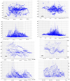 |
Fig. A.2 Same as Fig.6. |
| In the text | |
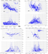 |
Fig. A.3 Same as Fig.6. |
| In the text | |
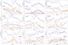 |
Fig. A.4 Same as Fig.7. |
| In the text | |
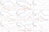 |
Fig. A.5 Same as Fig.7. |
| In the text | |
 |
Fig. A.6 Same as Fig.7. |
| In the text | |
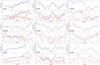 |
Fig. A.7 Same as Fig.7. |
| In the text | |
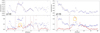 |
Fig. A.8 Same as Fig.7. |
| In the text | |
|
Fig. B.1 Average spectra in one beam size of 7 pixels for the off-position. |
| In the text | |
|
Fig. B.2 Noise maps of 13CO (3–2) and 12CO (3–2) in our observation. |
| In the text | |
|
Fig. B.3 Average spectra of one submap G333D55M-7M. |
| In the text | |
Current usage metrics show cumulative count of Article Views (full-text article views including HTML views, PDF and ePub downloads, according to the available data) and Abstracts Views on Vision4Press platform.
Data correspond to usage on the plateform after 2015. The current usage metrics is available 48-96 hours after online publication and is updated daily on week days.
Initial download of the metrics may take a while.