| Issue |
A&A
Volume 696, April 2025
|
|
|---|---|---|
| Article Number | L5 | |
| Number of page(s) | 7 | |
| Section | Letters to the Editor | |
| DOI | https://doi.org/10.1051/0004-6361/202453040 | |
| Published online | 07 April 2025 | |
Letter to the Editor
External tides: An important driver of velocity dispersion in molecular clouds
Max-Planck-Institut für Radioastronomie, Auf dem Hügel 69, 53121 Bonn, Germany
⋆ Corresponding author; This email address is being protected from spambots. You need JavaScript enabled to view it.
Received:
17
November
2024
Accepted:
20
March
2025
Abstract
Using the 3D density distribution derived from the 3D dust map of the solar neighborhood, the gravitational potential is obtained by solving the Poisson equation and the tidal tensor can then be computed. In optimal decomposition, the external tidal tensor follows the same formalism as that of a point mass. The average tidal strength of the clouds, derived from both tidal tensor analysis and pixel-by-pixel computation, shows consistent results. The equivalent velocity dispersion of the clouds, estimated from the average tidal strength, is comparable in magnitude to the velocity dispersion measured from CO (1–0) line emission. This suggests that tidal effects from surrounding material may play a significant role in driving velocity dispersion within the clouds. Future studies should carefully consider these tidal effects in star-forming regions.
Key words: ISM: clouds / dust, extinction / ISM: kinematics and dynamics / ISM: structure
© The Authors 2025
 Open Access article, published by EDP Sciences, under the terms of the Creative Commons Attribution License (https://creativecommons.org/licenses/by/4.0), which permits unrestricted use, distribution, and reproduction in any medium, provided the original work is properly cited.
This article is published in open access under the Subscribe to Open model.
Open access funding provided by Max Planck Society.
1. Introduction
One prevailing paradigm about star formation is that the collapse of gas is driven by gravity and balanced by processes such as turbulence and magnetic fields (McKee & Ostriker 2007). Based on this picture, the virial parameter (Bertoldi & McKee 1992) is always used to determine whether a structure is in a state of gravitational collapse. However, as pointed out in Ramírez-Galeano et al. (2022), Li (2024), studies usually focus on the role of gravity in individual, isolated parts and thus neglect long-range gravitational interactions. Diverse manifestations of gravitational effects on gas within molecular clouds were unveiled in Li (2024). Gravity influences cloud evolution in various ways. Within dense regions, it facilitates fragmentation and collapse. Outside these regions, it can suppress the collapse of low-density gas through extensive tidal forces and drive accretion.
Star-forming regions typically exhibit hierarchical gas structures. High-mass stars preferentially form in the density enhanced hubs of hub-filament systems (Myers 2009; Schneider et al. 2012; Motte et al. 2018; Kumar et al. 2020; Zhou et al. 2022). The hub can drive longitudinal gas inflows along filaments, providing further mass accretion (Peretto et al. 2013; Henshaw et al. 2014; Zhang et al. 2015; Yuan et al. 2018; Lu et al. 2018; Issac et al. 2019; Dewangan et al. 2020; Liu et al. 2016, 2021b, 2022; Liu et al. 2023; Kumar et al. 2020; Zhou et al. 2022; Xu et al. 2023; Zhou et al. 2023; Yang et al. 2023; Zhou et al. 2024b). Zhou et al. (2022) examined the physical properties and evolution of hub-filament systems in roughly 140 clumps using spectral line data from the ALMA Three-millimeter Observations of Massive Star-forming regions (ATOMS) survey (Liu et al. 2020). We proposed that hub-filament structures, characterized by self-similarity and filamentary accretion, are consistent across different scales in high-mass star-forming regions, spanning from a few thousand astronomical units to several parsecs. This picture of hierarchical, multi-scale hub-filament structures was expanded from the clump-core scale to the cloud-clump scale by Zhou et al. (2023) and later extended to the galaxy-cloud scale in Zhou & Davis (2024), Zhou et al. (2024a), Zhou & Li (2025). Previous works have also demonstrated hierarchical collapse and the feeding of central regions by hub-filament structures, including Motte et al. (2018), Vázquez-Semadeni et al. (2019), Kumar et al. (2020), and references therein.
Gravity is a long-range force. A local gas structure evolves under its self-gravity, but as a gravitational center, its influence can also affect neighboring structures. At the same time, it also experiences external gravity from neighboring material. Tidal and gravitational fields are mutually interdependent. Tidal forces have been proposed in previous studies as a factor that can either regulate or initiate star formation. Ballesteros-Paredes et al. (2009b,a) examined the effects of tidal forces induced by the Galactic potential on molecular clouds and demonstrated that these forces can either compress or disrupt the clouds, thereby impacting star-formation efficiency. For M 51 and NGC 4429, the models of Meidt et al. (2018), Liu et al. (2021a) investigated the influence of the host galaxy potential on molecular clouds, showing that cloud-scale gas dynamics result from the interplay between the galactic potential and gas self-gravity, which plays a key role in shaping molecular cloud properties. However, for the Large Magellanic Cloud (LMC), Thilliez et al. (2014) found that tidal instability does not hinder star formation. Furthermore, studies by Dib et al. (2012), Thilliez et al. (2014), Zhou & Dib (2025) have indicated that for molecular clouds in the Milky Way, the LMC, and NGC 628, the shear derived from the galactic rotation curve is negligible. Ramírez-Galeano et al. (2022) also suggest that tidal stresses from nearby molecular cloud complexes contribute more to interstellar turbulence than the overall galactic potential. The hierarchical, multi-scale hub-filament structures indicate that there are extensive tidal interactions in the interstellar medium (ISM). Regardless of whether the galactic potential influences molecular clouds and their complexes, these clouds are inevitably impacted by the cumulative tidal interactions with surrounding material. Such interactions may hinder gravitational collapse, suppress instability growth, and inhibit star formation within the cloud. Zhou & Dib (2025) carried out an examination of large-scale galactic effects on molecular cloud properties in NGC 628 and found a significant impact of tidal effects from neighboring material on the evolution of molecular clouds. The tidal effects from neighboring material may also be a significant contributing factor to the slowing down of a pure free-fall gravitational collapse for gas structures on galaxy-cloud scales revealed by velocity gradient measurements (Zhou & Davis 2024; Zhou et al. 2024a). In Zhou et al. (2024b), it was shown that the deformation due to the external tides can also effectively slow down the pure free-fall gravitational collapse of gas structures on clump-core scales. These mechanisms could be called “tide-regulated gravitational collapse.”
Due to the diffuse and complex morphology of the ISM, a complete tidal calculation would be complex. One should derive the gravitational potential distribution from the 3D density distribution and then calculate the tidal field according to the gravitational potential, as presented in Li (2024). In observations, one can usually only obtain the 2D projected surface density map. However, building on the accurate distances enabled in the Gaia era, we have been able to infer the 3D density distribution of the ISM by the 3D dust mapping technique (Rezaei et al. 2018; Chen et al. 2019; Green et al. 2019; Lallement et al. 2019; Hottier et al. 2020; Leike et al. 2020; Edenhofer et al. 2024). In this work, we first calculate and decompose the tidal field using the 3D dust map and then explore methods to estimate the tidal strength within the clouds induced by external gravity. Finally, we assess the impact of external tides on the physical properties of molecular clouds.
2. Data
2.1. 3D dust map
Edenhofer et al. (2024) offers the most accurate 3D dust map to date for the solar neighborhood within 1.25 kpc, employing a novel Gaussian process prior approach to reduce the impact of fingers-of-god artifacts. This 3D map was generated using stellar distance and extinction estimates from Zhang et al. (2023) derived from Gaia spectra. There are 12 samples from their inferred 3D dust extinction distribution. In this work, our calculation is based on the posterior mean of their reconstruction, which is the average of these 12 samples. Using the method described in O’Neill et al. (2024), we converted the differential extinction in the 3D map to the number density of hydrogen nuclei, n, independent of phase (n = nHI + 2nH2). The volume density is then ρ = 1.37mpn, where mp represents the mass of a proton and the factor 1.37 accounts for the contribution of helium to the total mass based on cosmic abundance ratios relative to hydrogen.
2.2. CO (1−0) line emission
We also utilized the full position–position–velocity (l − b − v) cube of CO1 from Dame et al. (2001). The spatial range of this cube is all Galactic longitudes and ±300 Galactic latitude. The velocity range is ±320 km s−1.
3. Results
3.1. Structural identification
Fig. 1a shows the surface density map of hydrogen nuclei on the l − b plane. We applied the dendrogram algorithm to identify the local dense structures based on this surface density map. Then the CO (1−0) cube was utilized to derive the velocity dispersion of the identified structures. Since the CO (1−0) cube is in the Galactic coordinates (l − b − v), we also used the 3D dust map provided in the Galactic coordinate system (l − b − d)2. This allowed both cubes to be analyzed in the same way, as they have the same data structure.
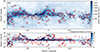 |
Fig. 1. Structural identification. (a) Surface density of hydrogen nuclei on the l − b plane. Red contours are the structures identified by the dendrogram algorithm. (b) Integrated intensity map of CO (1−0) line emission. Red contours are the same as in panel (a). |
As described in Rosolowsky et al. (2008), the dendrogram algorithm decomposes density data into hierarchical structures. Using the astrodendro package3, there are three major input parameters for the dendrogram algorithm: min_value for the minimum value to be considered in the dataset, min_delta for a leaf that can be considered as an independent entity, and min_npix for the minimum area of a structure. In this work, we took the values of min_value = 5 * Σrms and min_delta = 5 * Σrms, where Σrms is the average density of the background on the map shown in Fig. 1a. After testing different values, we set min_npix = 100 pixels to ensure that the identified structures are not too small. As shown in Fig. 1a, the structures identified by the dendrogram correspond well to the surface density distribution. In Fig. 1b, CO and dust also show a good correspondence in their distribution, but CO emission is primarily concentrated in the Galactic plane.
Using the mask of each identified structure in Fig. 1a, we extracted the average “spectra” according to the l − b − v and l − b − d cubes. Specifically, for each identified structure, we averaged the intensity or density values across all pixels within the masked region and analyzed the intensity distribution along the velocity axis and the density distribution along the distance axis, as shown in Fig. 2. This approach allowed us to investigate the characteristic velocity and distance distributions of the structures, thus providing insights into their kinematics and spatial properties. If an identified structure is a single structure without overlap, we would expect both types of “spectra” to exhibit a single peak, as shown in Fig. 2. In total, 90 structures satisfy this condition. From the “spectra,” the systematic velocity, the velocity dispersion (σg), the distance, and the thickness of each structure can be obtained. The thickness is the full width at half maximum of the line profile, displayed in Fig. 2a. The dendrogram algorithm approximates the morphology of each structure as an ellipse. Using the long and short axes (l1 and l2) of the effective ellipse and the half-thickness (l3), we estimated a 3D effective radius for each structure, R ≈ (l1 * l2 * l3)1/3.
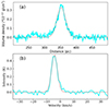 |
Fig. 2. Average “spectra” (cyan lines) of a single structure extracted from the l − b − v and l − b − d cubes, respectively. (a) Averaged intensity distribution along the velocity axis. (b) Averaged density distribution along the distance axis. Red dashed lines represent the Gaussian fitting. |
3.2. Tidal strength
In Appendix A, for a subregion of the 3D map, based on the 3D density distribution, the gravitational potential was computed by solving the Poisson equation. The tidal tensor was then derived from the gravitational potential. For a cloud, its tidal tensor can be divided into two parts (internal and external) due to the matter inside and outside the cloud. Different decomposition methods resulted in four possible maximum eigenvalues (|λext, max|) of the external tidal tensor (Text). An independent and original pixel-by-pixel computation method was used to select the optimal |λext, max|. For the eigenvalues, we found that the optimal Text shows the same formalism with the tidal tensor of a point mass. Therefore, for the external tides exerted by external material at a point within a cloud, the external material can be approximated as a collection of point masses. Each point mass generates its own tidal field. The combined effect of the external tides is equivalent to the superposition of the tidal fields produced by all these point masses. Essentially, this approach is analogous to the pixel-by-pixel computation. As shown in Fig. A.4, the average tidal strength in the clouds calculated by the two methods shows comparable results.
Our current computational resources are insufficient to directly calculate the tidal tensor of the entire 3D map. Therefore, we adopted the pixel-by-pixel computation approach to calculate the average tidal strength (λpp) of all structures in the subsequent analysis. This method only considers the structure being calculated and its neighboring matter each time. Typically, accounting for matter within eight to ten times the structure’s radius is sufficient, as tidal strength decreases rapidly with distance (Equation (A.10)).
3.3. Velocity dispersion
We estimated an equivalent velocity dispersion for the clouds according to the average tidal strength, as done in Zhou et al. (2024b). The tidal strength defined in this work is the tidal acceleration per unit distance (Stark & Blitz 1978). Thus, for a cloud with radius R and mass M, λpp * R is the tidal acceleration. The velocity dispersion of a gas structure measures the intensity of internal gas motion within the structure. The tides induced by external gravity pervade the interior of the gas structure. We propose that these ubiquitous gravitational differences serve as the driving force for the motion of gas parcels within the structure. The work done by tidal forces is converted into kinetic energy, which corresponds to the equivalent velocity dispersion, σt:
 (1)
(1)
We then have
 (2)
(2)
Since σt is derived from the average tidal strength over the entire structure, it is isotropic and can be directly compared to the observed velocity dispersion of the structure obtained in Sec. 3.1. As shown in Fig. 3, σt is roughly comparable with σg in magnitude, which means that tidal effects from external gravity can significantly contribute to the velocity dispersion of the clouds. A relatively smaller value of σt is also reasonable, as other physical processes (such as gravitational collapse and feedback activities) also contribute to the overall velocity dispersion of the cloud.
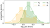 |
Fig. 3. Kernel density estimation and the histogram of the velocity dispersion of the clouds. The term σt is the equivalent velocity dispersion derived from the average tidal strength, and σg is the velocity dispersion measured from CO emission. |
4. Discussion and conclusions
The 3D density distribution derived from the 3D dust map is crucial for calculating the tidal field. However, velocity information is only available from the projected CO (1−0) line emission. To address this, we first projected the 3D density cube onto the l − b plane and then applied the dendrogram algorithm to identify the clouds. As shown in Fig. 1, the distributions of projected CO and dust emission exhibit a good correspondence. For 90 non-overlapping clouds, we fit the systematic velocity, velocity dispersion, distance, and thickness based on the average “spectra” extracted from the l − b − v and l − b − d cubes. These clouds were then used to study tidal effects. We employed two methods to estimate tidal strength, tidal tensor analysis and pixel-by-pixel computation, which produced comparable results. The equivalent velocity dispersion, derived from the average tidal strength, is roughly consistent in magnitude with the observed velocity dispersion, suggesting that tidal effects from external gravity play a significant role in shaping the velocity dispersion of the clouds. The significant impact of external gravity from the neighboring material on the physical properties of molecular clouds has also been demonstrated in Ramírez-Galeano et al. (2022), Li (2024), Zhou et al. (2024b), Zhou & Dib (2025). The extensive tides can produce turbulence, suppress fragmentation, and slow down gravitational collapse. Extended gas structures in the ISM are sensitive to the tidal effects exerted by surrounding material. Future studies should incorporate these tidal effects into star-formation theories. Star formation in molecular clouds typically occurs within locally dense clumps. It is essential to study these clumps in the context of their surrounding environment rather than in isolation, as their interactions with the surrounding material cannot be ignored.
As shown in Appendix A, the calculation of tidal strength is based on density. In this work, we adopted the method described in O’Neill et al. (2024) to convert the differential extinction in the 3D dust map to the density of hydrogen nuclei. However, this method relies on certain assumptions, such as a constant ratio of hydrogen column density to extinction. To achieve a more accurate calculation of tidal strength, better estimates of both the density distribution and magnitude will be essential.
References
- Ballesteros-Paredes, J., Gómez, G. C., Loinard, L., Torres, R. M., & Pichardo, B. 2009a, MNRAS, 395, L81 [NASA ADS] [Google Scholar]
- Ballesteros-Paredes, J., Gómez, G. C., Pichardo, B., & Vázquez-Semadeni, E. 2009b, MNRAS, 393, 1563 [NASA ADS] [Google Scholar]
- Bertoldi, F., & McKee, C. F. 1992, ApJ, 395, 140 [NASA ADS] [CrossRef] [Google Scholar]
- Chen, B. Q., Huang, Y., Yuan, H. B., et al. 2019, MNRAS, 483, 4277 [Google Scholar]
- Dame, T. M., Hartmann, D., & Thaddeus, P. 2001, ApJ, 547, 792 [Google Scholar]
- Dewangan, L. K., Ojha, D. K., Sharma, S., et al. 2020, ApJ, 903, 13 [Google Scholar]
- Dib, S., Helou, G., Moore, T. J. T., Urquhart, J. S., & Dariush, A. 2012, ApJ, 758, 125 [NASA ADS] [CrossRef] [Google Scholar]
- Edenhofer, G., Zucker, C., Frank, P., et al. 2024, A&A, 685, A82 [NASA ADS] [CrossRef] [EDP Sciences] [Google Scholar]
- Ganguly, S., Walch, S., Clarke, S. D., & Seifried, D. 2024, MNRAS, 528, 3630 [NASA ADS] [CrossRef] [Google Scholar]
- Green, G. M., Schlafly, E., Zucker, C., Speagle, J. S., & Finkbeiner, D. 2019, ApJ, 887, 93 [NASA ADS] [CrossRef] [Google Scholar]
- Henshaw, J. D., Caselli, P., Fontani, F., Jiménez-Serra, I., & Tan, J. C. 2014, MNRAS, 440, 2860 [Google Scholar]
- Hottier, C., Babusiaux, C., & Arenou, F. 2020, A&A, 641, A79 [NASA ADS] [CrossRef] [EDP Sciences] [Google Scholar]
- Issac, N., Tej, A., Liu, T., et al. 2019, MNRAS, 485, 1775 [NASA ADS] [CrossRef] [Google Scholar]
- Kumar, M. S. N., Palmeirim, P., Arzoumanian, D., & Inutsuka, S. I. 2020, A&A, 642, A87 [EDP Sciences] [Google Scholar]
- Lallement, R., Babusiaux, C., Vergely, J. L., et al. 2019, A&A, 625, A135 [NASA ADS] [CrossRef] [EDP Sciences] [Google Scholar]
- Leike, R. H., Glatzle, M., & Enßlin, T. A. 2020, A&A, 639, A138 [NASA ADS] [CrossRef] [EDP Sciences] [Google Scholar]
- Li, G.-X. 2024, MNRAS, 528, L52 [Google Scholar]
- Liu, T., Zhang, Q., Kim, K.-T., et al. 2016, ApJ, 824, 31 [Google Scholar]
- Liu, T., Evans, N. J., Kim, K.-T., et al. 2020, MNRAS, 496, 2790 [Google Scholar]
- Liu, L., Bureau, M., Blitz, L., et al. 2021a, MNRAS, 505, 4048 [NASA ADS] [CrossRef] [Google Scholar]
- Liu, X.-L., Xu, J.-L., Wang, J.-J., et al. 2021b, A&A, 646, A137 [NASA ADS] [CrossRef] [EDP Sciences] [Google Scholar]
- Liu, H.-L., Tej, A., Liu, T., et al. 2022, MNRAS, 511, 4480 [NASA ADS] [CrossRef] [Google Scholar]
- Liu, H.-L., Tej, A., Liu, T., et al. 2023, MNRAS, 522, 3719 [NASA ADS] [CrossRef] [Google Scholar]
- Lu, X., Zhang, Q., Liu, H. B., et al. 2018, ApJ, 855, 9 [Google Scholar]
- McKee, C. F., & Ostriker, E. C. 2007, ARA&A, 45, 565 [Google Scholar]
- Meidt, S. E., Leroy, A. K., Rosolowsky, E., et al. 2018, ApJ, 854, 100 [NASA ADS] [CrossRef] [Google Scholar]
- Motte, F., Bontemps, S., & Louvet, F. 2018, ARA&A, 56, 41 [NASA ADS] [CrossRef] [Google Scholar]
- Myers, P. C. 2009, ApJ, 700, 1609 [Google Scholar]
- O’Neill, T. J., Zucker, C., Goodman, A. A., & Edenhofer, G. 2024, ApJ, 973, 136 [NASA ADS] [CrossRef] [Google Scholar]
- Peretto, N., Fuller, G. A., Duarte-Cabral, A., et al. 2013, A&A, 555, A112 [NASA ADS] [CrossRef] [EDP Sciences] [Google Scholar]
- Ramírez-Galeano, L., Ballesteros-Paredes, J., Smith, R. J., Camacho, V., & Zamora-Avilés, M. 2022, MNRAS, 515, 2822 [CrossRef] [Google Scholar]
- Rezaei, K. S., Bailer-Jones, C. A. L., Hogg, D. W., & Schultheis, M. 2018, A&A, 618, A168 [NASA ADS] [CrossRef] [EDP Sciences] [Google Scholar]
- Rosolowsky, E. W., Pineda, J. E., Kauffmann, J., & Goodman, A. A. 2008, ApJ, 679, 1338 [Google Scholar]
- Schneider, N., Csengeri, T., Hennemann, M., et al. 2012, A&A, 540, L11 [NASA ADS] [CrossRef] [EDP Sciences] [Google Scholar]
- Stark, A. A., & Blitz, L. 1978, ApJ, 225, L15 [NASA ADS] [CrossRef] [Google Scholar]
- Thilliez, E., Maddison, S. T., Hughes, A., & Wong, T. 2014, PASA, 31, e003 [Google Scholar]
- Vázquez-Semadeni, E., Palau, A., Ballesteros-Paredes, J., Gómez, G. C., & Zamora-Avilés, M. 2019, MNRAS, 490, 3061 [Google Scholar]
- Xu, F.-W., Wang, K., Liu, T., et al. 2023, MNRAS, 520, 3259 [NASA ADS] [CrossRef] [Google Scholar]
- Yang, D., Liu, H.-L., Tej, A., et al. 2023, ApJ, 953, 40 [NASA ADS] [CrossRef] [Google Scholar]
- Yuan, J., Li, J.-Z., Wu, Y., et al. 2018, ApJ, 852, 12 [Google Scholar]
- Zhang, Q., Wang, K., Lu, X., & Jiménez-Serra, I. 2015, ApJ, 804, 141 [Google Scholar]
- Zhang, X., Green, G. M., & Rix, H.-W. 2023, MNRAS, 524, 1855 [NASA ADS] [CrossRef] [Google Scholar]
- Zhou, J.-W., & Davis, T. 2024, PASA, 41 [Google Scholar]
- Zhou, J. W., & Dib, S. 2025, MNRAS, 537, 2232 [NASA ADS] [CrossRef] [Google Scholar]
- Zhou, J. W., & Li, G.-X. 2025, MNRAS, 537, 2630 [NASA ADS] [CrossRef] [Google Scholar]
- Zhou, J.-W., Liu, T., Evans, N. J., et al. 2022, MNRAS, 514, 6038 [NASA ADS] [CrossRef] [Google Scholar]
- Zhou, J. W., Wyrowski, F., Neupane, S., et al. 2023, A&A, 676, A69 [NASA ADS] [CrossRef] [EDP Sciences] [Google Scholar]
- Zhou, J. W., Dib, S., & Davis, T. A. 2024a, MNRAS, 534, 683 [NASA ADS] [CrossRef] [Google Scholar]
- Zhou, J. W., Dib, S., Juvela, M., et al. 2024b, A&A, 686, A146 [NASA ADS] [CrossRef] [EDP Sciences] [Google Scholar]
Appendix A: Tidal calculation
A.1. Tidal tensor
In the tidal tensor computation, we utilized the 3D dust map available in the heliocentric Galactic Cartesian coordinate system (X-Y-Z).4 Based on the 3D density distribution derived from the 3D dust map, the gravitational potential is computed by solving the Poisson equation ∇2ϕ = 4πGρ in the Fourier space,
 (A.1)
(A.1)
where we first calculate  . The gravitational potential in the real space is then computed through
  . The terms
  and
and  are the Fourier transform and the inverse Fourier transform. For a gravitational potential field Φ, the tidal tensor T is defined as
 (A.2)
(A.2)
The tidal tensor is symmetric and real-valued. Thus, it can be written in orthogonal form. The ordered and diagonalized tidal tensor is given as
 (A.3)
(A.3)
The eigenvalues of the tidal tensor provide insight into gravitationally induced deformations, such as compression or disruption, at a given point within the gravitational field. The sign of an eigenvalue determines whether the corresponding mode is compressive (λi > 0) or disruptive (λi < 0), while its magnitude indicates the strength of the respective compressive or disruptive effect. The "ordered" means |λ3|> |λ2|> |λ1|. The trace of the tidal tensor,  , contains the local density information in the Poisson equation:
 (A.4)
(A.4)
This implies that the trace is 0 if the point at which the tidal tensor is evaluated outside the mass distribution.
Due to computational resource limitations, we focused our calculations on the subregion (X × Y × Z = 700 pc × 700 pc × 700 pc) outlined by the red box in Fig. A.1. Fig. A.2 displays a snapshot of the density and the maximum eigenvalue of the tidal tensor (λ3) on XY plane, when Z = 80 pc.
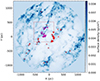 |
Fig. A.1. Surface density of hydrogen nuclei on the XY plane. The pluses represent the 90 non-overlapping structures in Sec. 3.1. |
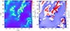 |
Fig. A.2. Tidal field in the heliocentric Galactic Cartesian coordinate system calculated based on the 3D dust distribution near the Sun. The Sun is located at the origin (0,0). Here, we present snapshots of the volume density and the maximum eigenvalue of the tidal tensor on the XY plane at Z = 80 pc. |
As discussed in Ganguly et al. (2024), the tidal tensor can be decomposed into three components: the tidal tensor generated solely by the matter within the structure, Tint; the tidal tensor arising exclusively from the external matter distribution, Text; and their sum, which represents the contribution from the entire matter distribution:
 (A.5)
(A.5)
Here, Ttot represents the net deformation due to both the structure itself and its external material. The traces of the three parts are
 (A.6)
(A.6)
 (A.7)
(A.7)
 (A.8)
(A.8)
The trace in equation.A.8 suggests that Text must include both compressive and disruptive modes, corresponding to positive and negative λi, respectively. In contrast, Tint and Ttot must contain at least one compressive mode but can also be entirely compressive. According to equation.A.5, the 3D tidal tensor can be decomposed as
 (A.9)
(A.9)
For the six unknown parameters, they satisfy the following four equations:
Since the six unknown parameters are real numbers, we set A4 = k * A5 and A1 = h * A2, where k and h are arbitrary constants, then we have the solutions of the unknown parameters:
The solutions require h ≠ k. Below, we consider several limiting cases:
1. When k ≫ 1 and h ≈ 1, the solutions of the six unknown parameters are A0 = −2λ3, A1 = λ3, A2 = λ3, A3 = λ1 + 2λ3, A4 = λ2 − λ3, A5 = 0.
2. When k ≫ 1 and h ≪ 1, the solutions of the six unknown parameters are A0 = −λ3, A1 = 0, A2 = λ3, A3 = λ1 + λ3, A4 = λ2, A5 = 0.
3. When k ≈ 1 and h ≫ 1, the solutions of the six unknown parameters are A0 = −λ2 + λ3, A1 = λ2 − λ3, A2 = 0, A3 = λ1 + λ2 − λ3, A4 = λ3, A5 = λ3.
4. When k ≈ 1 and h ≪ 1, the solutions of the six unknown parameters are A0 = λ2 − λ3, A1 = 0, A2 = −λ2 + λ3, A3 = λ1 − λ2 + λ3, A4 = λ2, A5 = λ2.
5. When k ≪ 1 and h ≫ 1, the solutions of the six unknown parameters are A0 = −λ2, A1 = λ2, A2 = 0, A3 = λ1 + λ2, A4 = 0, A5 = λ3.
6. When k ≪ 1 and h ≈ 1, the solutions of the six unknown parameters are A0 = −2λ2, A1 = λ2, A2 = λ2, A3 = λ1 + 2λ2, A4 = 0, A5 = −λ2 + λ3.
Assuming that the largest eigenvalue of Text dominates the deformation of a given structure due to the external tides, in the six limiting cases, the maximum eigenvalue of Text (i.e., λext, max) can be | − 2λ2|, | − 2λ3|, |λ2 − λ3|, | − λ2|, and | − λ3|. Since the eigenvalues can become negative, we consider their absolute values in order to compare the relative magnitude. Similar to the case of A4 = k * A5 and A1 = h * A2, there are eight other situations:
A0 = h * A1 and A3 = k * A4,
A0 = h * A1 and A3 = k * A5,
A0 = h * A1 and A4 = k * A5,
A0 = h * A2 and A3 = k * A4,
A0 = h * A2 and A3 = k * A5,
A0 = h * A2 and A4 = k * A5,
A1 = h * A2 and A3 = k * A4,
A1 = h * A2 and A3 = k * A5.
For all limiting cases, there are 12 possible |λext, max|: | − 2λ1|, | − λ1|, | − 2λ2|, | − λ2|, | − 2λ3|, | − λ3|, |λ1 − λ2|, |λ1 − λ3|, |λ2 − λ3|, |λ1 − λ2|/2, |λ1 − λ3|/2, and |λ2 − λ3|/2. Since |λ3|> |λ2|> |λ1|, we only need to consider four of them, namely: | − 2λ3|, |λ1 − λ2|, |λ1 − λ3|, and |λ2 − λ3|.
A.2. Pixel-by-pixel computation
Below, we introduce an independent and original method to select the optimal |λext, max| from four possible ones. At a distance R′ from a pixel B with mass M′, the tidal strength sustained by a pixel A due to the external gravity of pixel B is
 (A.10)
The cumulative tidal strength at a pixel signifies the aggregate deformation resulting from external gravity at that point. Unlike a rigid body or a point-mass, a gas structure is flexible and can be deformed. Gas structures are often irregular in shape, and their morphologies can be quite intricate. While the gravitational forces acting on a gas structure from different directions might balance out, the tidal effects within the structure, driven by external gravity, do not. To quantify the collective tidal strength within a gas structure induced by external gravity, we adopt the scalar superposition. According to the central coordinates (X, Y and Z) and radius of each cloud identified in Sec. 3.1, we can divide the 3D density cube into two parts, i.e. the cloud itself and all external material apart from this cloud. For the external tides from external material sustained by a point in the cloud, a simple but heavy calculation is using equation.A.10 to directly calculate the tidal strength at that point pixel-by-pixel through the entire cube, as illustrated in Fig. A.3. Fig. A.4 shows the distribution of the average tidal strengths (four possible |λext, max| and the pixel-by-pixel computed one, i.e. λpp) for the clouds marked by magenta "+" within the box of Fig. A.1. Since the clouds at the boundary cannot account for all neighboring material, they were excluded. The distribution of | − 2λ3| is closest to λpp. In equation.A.9, when A0 = −2λ3, we obtain a decomposition of the tidal tensor:
 (A.11)
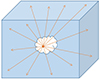 |
Fig. A.3. Pixel-by-pixel computation. Here, we took out a cloud from the 3D density cube and calculated the external tides from all external material at a point in the cloud. |
For a point-mass with mass M0, the tidal tensor at distance d is given as
 (A.12)
As shown in Fig. A.4, < |2λ3|> ≈ < 2GM′/R′3> (equation.A.10), and the eigenvalues of Text in equation.A.11 has the same formalism with the tidal tensor of a point-mass. Therefore, for the external tides from external material sustained by a point in a cloud, the external material can be divided into approximate point-masses. Each point-mass can produce its own tidal field. The external tides from all external material are equivalent to the superposition of the tidal fields of all divided point-masses. In essence, it is equivalent to the above pixel-by-pixel computation.
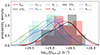 |
Fig. A.4. Kernel density estimation and the histogram of the average external tidal strength of the clouds. Here, | − 2λ3|, |λ1 − λ2|, |λ1 − λ3|, and |λ2 − λ3| are four possible maximum eigenvalues derived in Sec. A.1, and λpp is the tidal strength from the pixel-by-pixel computation. The comparison is only conducted on the clouds marked by a magenta "+" within the box of Fig. A.1. |
All Figures
|
Fig. 1. Structural identification. (a) Surface density of hydrogen nuclei on the l − b plane. Red contours are the structures identified by the dendrogram algorithm. (b) Integrated intensity map of CO (1−0) line emission. Red contours are the same as in panel (a). |
| In the text | |
|
Fig. 2. Average “spectra” (cyan lines) of a single structure extracted from the l − b − v and l − b − d cubes, respectively. (a) Averaged intensity distribution along the velocity axis. (b) Averaged density distribution along the distance axis. Red dashed lines represent the Gaussian fitting. |
| In the text | |
|
Fig. 3. Kernel density estimation and the histogram of the velocity dispersion of the clouds. The term σt is the equivalent velocity dispersion derived from the average tidal strength, and σg is the velocity dispersion measured from CO emission. |
| In the text | |
|
Fig. A.1. Surface density of hydrogen nuclei on the XY plane. The pluses represent the 90 non-overlapping structures in Sec. 3.1. |
| In the text | |
|
Fig. A.2. Tidal field in the heliocentric Galactic Cartesian coordinate system calculated based on the 3D dust distribution near the Sun. The Sun is located at the origin (0,0). Here, we present snapshots of the volume density and the maximum eigenvalue of the tidal tensor on the XY plane at Z = 80 pc. |
| In the text | |
|
Fig. A.3. Pixel-by-pixel computation. Here, we took out a cloud from the 3D density cube and calculated the external tides from all external material at a point in the cloud. |
| In the text | |
|
Fig. A.4. Kernel density estimation and the histogram of the average external tidal strength of the clouds. Here, | − 2λ3|, |λ1 − λ2|, |λ1 − λ3|, and |λ2 − λ3| are four possible maximum eigenvalues derived in Sec. A.1, and λpp is the tidal strength from the pixel-by-pixel computation. The comparison is only conducted on the clouds marked by a magenta "+" within the box of Fig. A.1. |
| In the text | |
Current usage metrics show cumulative count of Article Views (full-text article views including HTML views, PDF and ePub downloads, according to the available data) and Abstracts Views on Vision4Press platform.
Data correspond to usage on the plateform after 2015. The current usage metrics is available 48-96 hours after online publication and is updated daily on week days.
Initial download of the metrics may take a while.