| Issue |
A&A
Volume 686, June 2024
|
|
|---|---|---|
| Article Number | A13 | |
| Number of page(s) | 24 | |
| Section | Stellar structure and evolution | |
| DOI | https://doi.org/10.1051/0004-6361/202348790 | |
| Published online | 24 May 2024 | |
SN 2020pvb: A Type IIn-P supernova with a precursor outburst
1
INAF – Osservatorio Astronomico di Padova, vicolo dell’Osservatorio 5, Padova 35122, Italy
e-mail: This email address is being protected from spambots. You need JavaScript enabled to view it.
2
Institute of Space Sciences (ICE, CSIC), Campus UAB, Carrer de Can Magrans s/n, 08193 Barcelona, Spain
3
The Oskar Klein Centre, Department of Astronomy, Stockholm University, AlbaNova, 10691 Stockholm, Sweden
4
School of Physics, O’Brien Centre for Science North, University College Dublin, Belfield, Dublin 4, Ireland
5
Heidelberger Institut für Theoretische Studien, Schloss-Wolfsbrunnenweg 35, 69118 Heidelberg, Germany
6
European Southern Observatory, Alonso de Córdova 3107, Casilla 19, Santiago, Chile
7
Millennium Institute of Astrophysics (MAS), Nuncio Monseñor Sótero Sanz 100, Off. 104, Providencia, Santiago, Chile
8
Yunnan Observatories, Chinese Academy of Sciences, Kunming 650216, PR China
9
Key Laboratory for the Structure and Evolution of Celestial Objects, Chinese Academy of Sciences, Kunming 650216, PR China
10
International Centre of Supernovae, Yunnan Key Laboratory, Kunming 650216, PR China
11
Graduate Institute of Astronomy, National Central University, 300 Jhongda Road, 32001 Jhongli, Taiwan
12
CNRS, Institut d’Astrophysique de Paris (IAP) and Sorbonne Université (Paris 6), 98bis, Boulevard Arago, 75014 Paris, France
13
Astronomical Observatory, University of Warsaw, Al. Ujazdowskie 4, 00-478 Warszawa, Poland
14
Institut d’Estudis Espacials de Catalunya (IEEC), 08034 Barcelona, Spain
15
Cardiff Hub for Astrophysics Research and Technology, School of Physics & Astronomy, Cardiff University, Queens Buildings, The Parade, Cardiff CF24 3AA, UK
16
Tuorla Observatory, Department of Physics and Astronomy, University of Turku, 20014 Turku, Finland
17
Turku Collegium for Science, Medicine and Technology, University of Turku, 20014 Turku, Finland
18
School of Sciences, European University Cyprus, Diogenes street, Engomi, 1516 Nicosia, Cyprus
19
Instituto de Alta Investigación, Universidad de Tarapacá, Casilla 7D, Arica, Chile
20
INAF, Osservatorio Astronomico di Brera, Via E. Bianchi 46, 23807 Merate (LC), Italy
21
Cosmic DAWN Centre, Niels Bohr Institute, University of Copenhagen, Jagtvej 128, 2200 København N, Denmark
22
Department of Physics, University of Oxford, Denys Wilkinson Building, Keble Road, Oxford OX1 3RH, UK
23
Astrophysics Research Centre, School of Mathematics and Physics, Queen’s University Belfast, Belfast BT7 1NN, UK
24
INAF – Osservatorio Astronomico d’Abruzzo, Via M. Maggini snc, Teramo 64100, Italy
25
Institute for Astronomy, University of Hawaii, 2680 Woodlawn Drive, Honolulu, HI 96822, USA
26
Department of Particle Physics and Astrophysics, Weizmann Institute of Science, 76100 Rehovot, Israel
27
Gran Telescopio Canarias (GRANTECAN), Cuesta de San José s/n, 38712 Breña Baja, La Palma, Spain
28
Instituto de Astrofísica de Canarias, Vía Láctea s/n, 38200 La Laguna, Tenerife, Spain
29
Astrophysics Research Institute, Liverpool John Moores University, ic2, 146 Brownlow Hill, Liverpool L3 5RF, UK
30
Max-Planck Institut für Astrophysik, Karl-Schwarzschild-Str. 1, 85741 Garching bei München, Germany
31
INAF, Osservatorio Astronomico di Roma, Via Frascati 33, 00078 Monte Porzio Catone (RM), Italy
32
Space Science Data Center – ASI, Via del Politecnico SNC, 00133 Roma, Italy
33
Department of Physics and Astronomy, Johns Hopkins University, 3400 North Charles Street, Baltimore, MD 21218, USA
34
Space Telescope Science Institute, 3700 San Martin Drive, Baltimore, MD 21218, USA
Received:
30
November
2023
Accepted:
2
February
2024
Abstract
We present photometric and spectroscopic datasets for SN 2020pvb, a Type IIn-P supernova (SN) that is similar to SNe 1994W, 2005cl, 2009kn, and 2011ht, with a precursor outburst detected (PS1 w band ∼–13.8 mag) around four months before the B-band maximum light. SN 2020pvb presents a relatively bright light curve that peaked at MB = −17.95 ± 0.30 mag and a plateau that lasted at least 40 days before going into solar conjunction. After this, the object was no longer visible at phases > 150 days above –12.5 mag in the B band, suggesting that the SN 2020pvb ejecta interact with a dense, spatially confined circumstellar envelope. SN 2020pvb shows strong Balmer lines and a forest of Fe II lines with narrow P Cygni profiles in its spectra. Using archival images from the Hubble Space Telescope, we constrained the progenitor of SN 2020pvb to have a luminosity of log(L/L⊙)≲5.4, ruling out any single star progenitor over 50 M⊙. SN 2020pvb is a Type IIn-P whose progenitor star had an outburst ∼0.5 yr before the final explosion; the material lost during this outburst probably plays a role in shaping the physical properties of the SN.
Key words: supernovae: general / supernovae: individual: SN 2020pvb
© The Authors 2024
 Open Access article, published by EDP Sciences, under the terms of the Creative Commons Attribution License (https://creativecommons.org/licenses/by/4.0), which permits unrestricted use, distribution, and reproduction in any medium, provided the original work is properly cited.
This article is published in open access under the Subscribe to Open model. This email address is being protected from spambots. You need JavaScript enabled to view it. to support open access publication.
1. Introduction
Massive stars (≥8 M⊙) can lose mass via steady winds, binary interaction, or (more rarely) as a consequence of dramatic eruptions, which generate a dense and often structured circumstellar medium (CSM; Weis 2001; Vink 2008; Smith 2011, 2017a). In the case of single massive stars, non-terminal outbursts that can produce this CSM are instabilities occurring when the star approaches the end of its evolution. When such a massive star explodes as a supernova (SN), the ejected material interacts with the H-rich CSM. As a consequence, the resulting transient spectra present a blue continuum with superposed narrow emission lines – with inferred full-width-at-half-maximum (FWHM) velocities from a few tens to a few hundred km s−1 – that arise from the CSM excited by the shock interaction emission. The interaction can mask the innermost ejecta (as well as the explosion mechanism; Chevalier & Fransson 1994). However, if the CSM is optically thin or has a particular geometric configuration, it is also possible to detect high-velocity components (a few thousand km s−1) arising from the SN ejecta. These SNe are known as Type IIn SNe (named after the detection of narrow emission lines in their spectra; e.g. Schlegel 1990). Despite the similarity of their spectroscopic properties, SNe IIn light curves are quite heterogeneous, showing both slow- and fast-declining SNe as well as faint (MR ≲ −17 mag) and very bright (MR ≳ −19 mag) objects (e.g. Kiewe et al. 2012; Taddia et al. 2013; Nyholm et al. 2020).
Type IIn-P SNe (Mauerhan et al. 2013a; see also Smith 2017b; Fraser 2020) are a sub-class of SNe IIn that exhibit spectra with narrow emission lines throughout their evolution but have light curves with a well-defined plateau, mainly in the optical-red and near-infrared (NIR) bands (as in Type IIP SNe), followed by an abrupt drop (several magnitudes) onto a radioactive decay tail. Their post-plateau decay also suggests low ejected 56Ni masses and a low-energy explosion. The spectra of SNe IIn-P are characterised by a blue continuum and narrow Balmer emission lines together with a forest of narrow P Cygni Fe II lines, with no forbidden or high-ionisation lines. Specifically, narrow Balmer lines are visible during the earlier phase and are persistent for weeks or months, unlike those observed in very early SNe II (flash-ionisation features; e.g. Khazov et al. 2016; Bruch et al. 2021; Tartaglia et al. 2021). SN 1994W (Tsvetkov 1995; Cumming & Lundqvist 1997; Sollerman et al. 1998) is the prototype of the SNe IIn-P, and other well-studied cases include SNe 2009kn (Kankare et al. 2012), 2005cl (Kiewe et al. 2012), and 2011ht (Roming et al. 2012; Mauerhan et al. 2013a). We note that Smith (2013) proposed that the Crab Nebula may be the remnant of an event of this type, albeit with some uncertainties.
Type IIn SNe are suggested to originate from high luminosity, massive progenitors (e.g. Gal-Yam et al. 2007; Elias-Rosa et al. 2018), with cases of variability of the pre-SN precursor stars (∼25% of the SN IIn cases according to Strotjohann et al. 2021; e.g. Ofek et al. 2013, 2014a, 2016; Mauerhan et al. 2013b; Fraser et al. 2013a; Margutti et al. 2014; Tartaglia et al. 2016; Elias-Rosa et al. 2016; Thöne et al. 2017; Pastorello et al. 2018; Reguitti et al. 2019). On the other hand, SNe IIn-P have been suggested to originate from the core collapse of intermediate-mass (8–10 M⊙) stars (e.g. Sollerman et al. 1998), with only a pre-SN precursor observed in one event, SN 2011ht (Fraser et al. 2013a). Alternative scenarios for SNe IIn-P include an electron capture SN explosion from a super-asymptotic giant branch (AGB) star (Mauerhan et al. 2013a; Smith 2013), a non-terminal outburst (Dessart et al. 2009; Humphreys et al. 2012), a post-merger event (Pastorello et al. 2019), or even eruptive outbursts of lower-mass red supergiants (Li & Morozova 2022). Regardless, this type of event does not seem to be related to very high-mass stars (e.g. Smith 2013; Chugai 2016).
Although ongoing surveys have significantly increased the available sample of SNe, the number of SNe IIn-P remains small, limiting our understanding of these objects. Here we present the case of SN 2020pvb, a member of this family of SNe and the second with a precursor outburst detected around four months before the discovery. In the next section (Sect. 2), we provide a summary of the properties of SN 2020pvb and its host galaxy. Photometric and spectroscopic data are analysed in Sect. 3, and the results are presented in Sect. 4. We discuss the nature of the progenitor star in Sect. 5 and the nature of the SN in Sect. 6.
2. SN 2020pvb: Discovery, explosion, distance, and reddening
AT 2020pvb ( ,
,  ; J2000.0)1 was discovered on 2020 July 18.42 UT (MJD = 59048.42) by the Panoramic Survey Telescope and Rapid Response System (Pan-STARRS; Chambers et al. 2020, 2016; Magnier et al. 2020), with a PS1 w-band magnitude of w = 21.04 ± 0.18. It was followed by non-detections from different surveys until new and independent discoveries were reported several weeks later by the Asteroid Terrestrial-impact Last Alert System (ATLAS; Tonry et al. 2018; Smith et al. 2020) and the Zwicky Transient Facility (ZTF; Masci et al. 2019), indicating that the July discovery was rather a pre-SN outburst. The transient was finally classified by ZTF (Perley et al. 2020) as a Type IIn SN on 2020 October 15.07 UT.
The first detection of SN 2020pvb on the main rise of its SN-like light curve was obtained on 2020 September 07 (MJD = 59099.37, o = 19.28 ± 0.43 mag) by ATLAS, while the last non-detection was obtained two days before (MJD = 59097.39, o > 19.8 mag). We hence estimate the explosion epoch to be on MJD = 59098.38 ± 1.0 (2020 September 06).
SN 2020pvb is hosted in the barred spiral galaxy NGC 6993 (SB(r)cd2; de Vaucouleurs et al. 1991; see Fig. 1). The recessional velocity of the galaxy, corrected for the Local Group infall into the Virgo cluster (Mould et al. 2000) is vVir = 6074 ± 9 km s−1 (z = 0.02025 ± 0.00003). Assuming H0 = 73.2 ± 1.3 km s−1 Mpc−1 (Riess et al. 2021), we derive a distance of 83.0 ± 1.5 Mpc (μ = 34.6 ± 0.1 mag). This distance will be adopted throughout this paper.
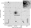 |
Fig. 1. NOT+ALFOSC image of the SN 2020pvb field in the r band obtained on 2020 October 15. The position of the SN is indicated with a circle, and a close-up of the area around the SN is shown in the upper-right inset. |
The Milky Way (MW) optical-band extinction in the direction of the transient is AV, MW = 0.187 mag (NED; Schlafly & Finkbeiner 2011). We find no evidence of Na I D absorption at the redshift of the host galaxy in our highest signal-to-noise (S/N) spectra, which would indicate the absence of gas, and hence likely dust, along the line of sight. Given the large dispersion observed in the equivalent width of the Na I D absorption lines versus E(B − V) plane (e.g. Elias-Rosa 2007; Poznanski et al. 2011; Phillips et al. 2013), we also estimated the optical extinction towards SN 2020pvb based on comparisons of the object’s spectral energy distribution (SED) with those of other Type IIn SNe with similar light curves or spectra (see Sect. 4). We first matched the intrinsic (B − V)0 colour curve of SN 2020pvb with those of SNe IIn-P 1994W (Tsvetkov 1995; Sollerman et al. 1998), 2009kn (Kankare et al. 2012), and 2011ht (Roming et al. 2012; Mauerhan et al. 2013a, see our Sect. 4.1). We compared the optical SED of SN 2020pvb at –24.3, 1.7, and 31.9 d from the B-band maximum with those of the previous comparison SNe at a similar epoch. The SED of the reference SNe were first corrected for redshift and extinction and then scaled to the distance of SN 2020pvb. Assuming RV = 3.1 (Cardelli et al. 1989), we derive an average AV, host = 0.15 mag, and thus we adopted AV = 0.34 ± 0.153 mag (i.e. E(B − V) = 0.11 ± 0.05 mag) as the total extinction towards SN 2020pvb.
3. Observations
3.1. Ground-based observations
Optical BV, ugriz, and NIR JHK images of SN 2020pvb were taken using a large number of observing facilities, listed in Table B.1. After its discovery, the transient was observed for about two months until it went behind the Sun. The telescopes pointed at the field again around two months later, but the SN was no longer visible with ground-based telescopes.
The photometric observations were reduced in the standard fashion with IRAF (Image Reduction and Analysis Facility) and various instrument pipelines. We performed photometry on SN 2020pvb and sequence stars using the Automated Photometry Of Transients pipeline (AUTOPHOT; Brennan & Fraser 2022). Point spread function (PSF) photometry was performed using a PSF model built from bright, isolated sources in the image. The optical magnitudes are calibrated against stars in the vicinity of SN 2020pvb with known Vega magnitudes from the American Association of Variable Star Observers (AAVSO) Photometric All-Sky Survey (APASS)4 and AB magnitudes from the Sloan Digital Sky Survey (SDSS)5. We have no sequence data for the R- and I-band images, and therefore we approximated the SN magnitudes using the Johnson-to-Sloan band transformation relations from Jester et al. (2005, see our Tables B.2 and B.3). For the NIR exposures, we also applied a sky background subtraction using the NOTCam QUICKLOOK v2.5 reduction package6 for the Nordic Optical Telescope (NOT) images and custom IDL (Interactive Data Language) routines for the CPAPIR images (Artigau et al. 2004). The NIR data are presented in Table B.4.
Late-time (phase > 150 d) photometry of SN 2020pvb was computed using the template-subtraction technique to remove the background and hence to measure more accurately the SN magnitudes. The template images were obtained with the New Technology Telescope+EFOSC27 at La Silla Observatory on 2021 September 15 through the extended Public ESO (European Southern Observatory) Spectroscopic Survey for Transient Objects (ePESSTO+) collaboration (Smartt et al. 2015). Each SN image was registered geometrically and photometrically with its corresponding template using the AUTOPHOT pipeline. We found the flux upper limits using a PSF model and artificial source injection at the position of SN 2020pvb, as described in Brennan & Fraser (2022).
Our dataset also includes photometry from the Pan-STARRS, ATLAS, and ZTF wide-field imaging surveys. We retrieved nine epochs of PS1 w-band photometry from the Pan-STARRS survey. The field was observed for five months before the SN was discovered. This photometry was obtained from the flux-weighted mean of each epoch in template-subtracted survey images. Two reference images were used, taken on MJD = 56 878.55 (2014 August 09) and MJD = 56 886.60 (2014 August 17). The final converted AB magnitudes and upper limits (corresponding to 3 times the standard deviation in the background) are listed in Table B.5.
ATLAS observed the SN field for five years before its discovery in cyan and orange (c and o) filters (broadly similar to g + r and r + i, respectively). We performed ATLAS forced photometry (Smith et al. 2020) at the site of SN 2020pvb using the host-galaxy template-subtraction technique. The reference images were taken on MJD = 58 661 (2019 June 27) in the ATLAS c band and MJD = 58 708 (2019 August 13) in the ATLAS o band. We computed a weighted mean of multiple exposures obtained at each epoch and then converted it to an AB magnitude. We present the final photometry in Table B.6.
ZTF photometry of SN 2020pvb was measured on gr-band template-subtracted images. The measurements were accessed through the forced photometry (Masci et al. 2019) released from the NASA/IPAC Infrared Science Archive8. This photometry is included in Table B.3.
Spectroscopic monitoring of SN 2020pvb started on 2020 October 12 and lasted two months. We collected 13 optical spectra9. All the spectra were obtained with the slit aligned along the parallactic angle to minimise differential flux losses caused by atmospheric refraction. The spectroscopic observational log can be found in Table B.710.
The spectra were reduced following standard procedures with IRAF routines via the graphical user interface FOSCGUI11 and the PESSTO pipeline (Smartt et al. 2015). The two-dimensional frames were corrected for bias and flat-fielded before the extraction of the one-dimensional spectra. The one-dimensional optical spectra were then wavelength calibrated by comparison with arc-lamp exposures obtained the same night, while the flux calibration was done using spectra of standard stars. We also verified the wavelength calibration against the bright night-sky emission lines and attempted to remove the strongest telluric absorption bands present in the spectra (in some cases, residuals are still present after the correction). Finally, the flux calibration of the reduced SN spectra was cross-checked against the broadband photometry, and flux scaled by a constant value when necessary.
3.2. Space telescope observations
The field of SN 2020pvb was also observed with the Neil Gehrels Swift Observatory (Gehrels et al. 2004) at four epochs with ultraviolet (UV) and optical filters. The magnitudes of the SN were measured using aperture photometry with the task UVOTSOURCE included in the Ultraviolet/Optical Telescope (UVOT) software package12. The derived magnitudes are listed in Tables B.8 and B.2.
The Hubble Space Telescope (HST) also observed the site of SN 2020pvb with the Wide Field Channel (WFC;  pixel−1) of the Advanced Camera for Surveys (ACS) in F606W (∼V band) on 2017 July 21 (SNAP-14840; PI A. Bellini), corresponding to 1092.5 days (3 yr) before the discovery of SN 2020pvb. The photometry of the stellar-like sources located near the transient position was obtained in the FLC frames (WFC-calibrated and corrected by charge transfer efficiency images) using DOLPHOT (Dolphin 2000, 2016) and choosing the drizzled frame as a reference. We used the recommended DOLPHOT parameter settings for ACS/WFC, considering both aperture sizes RAper = 4 and RAper = 8 for the photometry. We discuss this further in Sect. 5.
The field of SN 2020pvb was observed by the Galaxy Evolution Explorer (GALEX; Martin et al. 2005) as part of the All Sky Imaging Survey (ASIS) in both the near-UV (1800–2800 Å) and far-UV (1300–1800 Å) for a duration of 168 s on 2006 August 31. No point source is detected coincident with the position of the SN in either band. We estimate a 3σ upper limit of 19.7 and 20.4 mag (AB mag) for the near-UV and far-UV, respectively.
4. Results
4.1. Light curves
UV-optical-NIR light curves of SN 2020pvb are shown in Fig. 2. The light curves of the SN in all bands are characterised by a plateau-like phase at maximum light. This is reminiscent of the so-called SNe Type IIn-P (Mauerhan et al. 2013a).
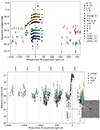 |
Fig. 2. Light curves of SN 2020pvb. Top: UV-optical-NIR light curves of SN 2020pvb. Upper limits are indicated by empty symbols with arrows. Bottom: Historical light curves of SN 2020pvb. Upper limits are indicated by empty symbols with arrows. The light curves have been shifted for clarity by the amounts indicated in the legend. The right insert is a 27″ × 27″ zoomed-in view of the transient position in the difference image (observation minus reference image) taken on 2020 July 18 in the PS1 w band. The precursor outburst is detected at a greater than 5-sigma significance. |
The optical light curves peak around 60 days after the estimated explosion date (this is best seen in the cyan and orange ATLAS curves), reaching a B-band maximum light on MJD = 59 159.18 ± 0.50. The long-lasting rise to the photometric peak is another characteristic of SN 2020pvb, in common with the SNe IIn-P. Moriya & Maeda (2014) proposed that the slow-rising light curve in interacting SNe results from the interaction with a dense CSM located at a large radius (see Sect. 5). We also note that the SN 2020pvb rise to the maximum light appears to be sharper in the bluer bands (also noted by Roming et al. 2012, for SN 2011ht). The u-band light curve in the top panel of Figs. 2 and A.1 increases by ∼1 mag from the time of the first observation until peak (in contrast to the ∼0.6 mag seen in the B-band light curve during the same time), and reaches the maximum ∼6 days earlier than that in the B band. Unfortunately, the NIR follow-up was sparse, and we cannot verify whether the rise is longer in these bands as reported by Mauerhan et al. (2013a) for SN 2011ht. We notice that late-NIR emission (> 400 d) was also detected in the case of the Type IIn-P SN 2009kn, probably due to early dust formation between 200 and 400 d (Kankare et al. 2012). However, we cannot confirm that this is a typical behaviour of Type IIn-P SNe, as no NIR data are available for other members of this sub-class. From our dataset, the SN 2020pvb plateau seems to be at least 40 days long from the SN maximum light. However, this is a lower limit because the transient went behind the Sun before the light curve dropped off. SNe IIn-P, such as SN 1994W, are expected to decline very rapidly after the plateau phase (see e.g. Chugai et al. 2004; Smith 2013; Chugai 2016) and follow a decline consistent with that of the radioactive 56Co decay. In fact, after the seasonal gap, the SN was below the detection threshold (> 22.9 mag in the r band).
The SN 2020pvb site was observed for several years before the SN discovery (Tables B.5, B.6 and bottom panel of Fig. 2). We did not detect a source at the event position brighter than the absolute magnitude –14.5 mag in the ATLAS bands or –12 mag in the PS1 w band, except for the single detection at an absolute magnitude of MPS1w ≈ −13.8 ± 0.5 mag on 2020 July 18 (the Pan-STARRS discovery, ∼111 d before the B-band maximum light and ∼50 days before the estimated explosion date), which we identified as a precursor outburst. This precursor is detected on four separate 45-s images on this night with no sign of motion for any of them, making the possibility of it being an asteroid unlikely. This source was not seen by the ATLAS survey in either the previous survey’s non-detection five days before the outburst or in the monthly stacked image from April to August 2020 down to a limiting magnitude of Mo ∼ −15 mag.
Figure 3 shows a comparison between the evolution of the absolute B magnitude of SN 2020pvb and those of the SNe IIn-P 1994W, 2005cl, 2009kn, 2011ht, and the ordinary SN IIP 2004et (Maguire et al. 2010) that has a similar luminosity to the general IIn-P population. The comparison SNe have been corrected for extinction using published estimates, assuming the Cardelli et al. (1989) extinction law and their respective kinematic distances were scaled assuming H0 = 73.2 ± 1.3 km s−1 Mpc−1. SN 2020pvb exhibits a broad light curve, similar to those of the SN 1994W-like SNe. This plateau, and the following decline, are different from that of a typical Type IIP such as SN 2004et (Fig. 3). The absolute B magnitude at the maximum of SN 2020pvb is −17.95 ± 0.30 mag, that is, between SN 1994W and SN 2011ht and approximately 1.2 mag fainter than SN 2005cl.
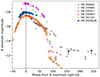 |
Fig. 3. Absolute B light curve of SN 2020pvb, shown together with those of SNe 1994W, 2005cl, 2009kn, 2011ht, and the Type IIP SN 2004et. Upper limits are indicated by vertical arrows. The dot-dashed vertical line indicates the B-band maximum light. The uncertainties for most data points are smaller than the plotted symbols. |
The (B − V)0 colour curve of SN 2020pvb (see Fig. 4) seems to evolve from red to blue at early times, followed by a flattening during the plateau phase and then gradually reddens. By the end of the plateau, SN 2020pvb shows a similar colour trend as SNe 1994W, 2005cl, 2009kn, and 2011ht, and yet is bluer than SN 2004et. The small evolution in the (B − V)0 reflects the SED temperature, which appears to be constant (see Sect. 4.2).
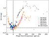 |
Fig. 4. Intrinsic colour evolution of SN 2020pvb, compared with those of SNe 1994W, 2005cl, 2009kn, 2011ht, and the Type IIP SN 2004et. The dot-dashed vertical line indicates the B-band maximum light of SN 2020pvb. |
We computed the pseudo-bolometric light curve of SN 2020pvb, and the comparison SNe, by integrating the flux from the extinction-corrected optical-NIR magnitudes. Fluxes were measured at epochs when B-band observations were available. When photometric measurements in one band at given epochs were not available, the flux was estimated by interpolating magnitudes from epochs close in time or, when necessary, by extrapolating the missing photometry assuming a constant colour. We estimated the pseudo-bolometric flux at each epoch by integrating the SED using the trapezoidal rule and assuming zero flux outside the integration boundaries. Finally, the effective fluxes were converted to luminosities using the adopted distance to the SN (see Sect. 2). The bolometric luminosity errors include the uncertainties in the distance estimate, the extinction, and the apparent magnitudes. As shown in Fig. 5, the pseudo-bolometric plateau of SN 2020pvb is similar in shape to SN 1994W-like SNe, although more luminous, except for SN 2005cl. Fitting low-order polynomials to the light curve, we estimate a peak luminosity of 4.8 ± 0.6 × 1042 erg s−1. We also include in the figure the pseudo-bolometric light curve of SN 2020pvb, including the UV data. This wavelength range contributes ∼25% to the SN luminosity. We note, however, that UV photometry is available only at two epochs near maximum light.
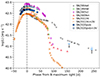 |
Fig. 5. Pseudo-bolometric light curve of SN 2020pvb obtained by integrating optical and NIR bands, compared with those of SNe 1994W, 2005cl, 2009kn, 2011ht, and the Type IIP SN 2004et. The UV-optical-NIR pseudo-bolometric light curve of SN 2020pvb is also included. The dot-dashed vertical line indicates the B-band maximum light of SN 2020pvb. |
4.2. Spectral evolution
Figure 6 shows the spectral evolution of SN 2020pvb. In Fig. 7 we superpose the second spectrum of SN 2020pvb (taken during the rise time at phase –21.3 d) and the last one (taken at 30.9 d, during the decline).
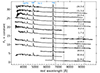 |
Fig. 6. Spectral sequence of SN 2020pvb extending from –24.3 d to 31.9 d from maximum light. All spectra have been corrected by redshift. The shaded wavelength regions indicate areas of strong telluric absorption, which has been removed when possible. The locations of the most prominent spectral features are also indicated. |
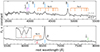 |
Fig. 7. Superposition of the 2020 October 15.88 UTC (–21.3 d, solid grey line) and 2020 December 08.03 UTC (31.9 d, dotted black line) spectra of SN 2020pvb. The insert is a zoomed-in view of the absorptions between 6300 and 6400 Å. The most prominent spectral features are indicated. |
The spectra of SN 2020pvb exhibit a blue continuum with very little evolution (note the similarity in features and line velocities among the spectra of Fig. 7). They are dominated by multi-component Balmer lines in emission and many Fe II features with narrow P Cygni profiles. Ca II H&K λλ3933,3968 features are visible in the first spectrum and throughout the plateau. In the red part of the spectra, it is noteworthy the complete absence of the Ca II NIR triplet, features almost always seen in both IIn and IIP SNe. Only a weak feature, possibly O Iλ7774, is visible. We also notice two small non-identified absorptions between 6300 and 6400 Å present in all spectra. We searched for typical SN lines, for example Fe II and/or Sc II features, but we did not find any convincing identification. One possible identification is with Si IIλλ6347,6371 also present in SN 1994W spectra from 21 to 89 d after its explosion (Chugai et al. 2004). Alternatively, we also considered the possibility that these absorptions were diffuse interstellar bands (DIBs), although they do not coincide with any of the DIBs listed in Herbig (1995) or Fan et al. (2019). Moreover, DIB intensity is correlated with the column density of Na I in the line of sight (Herbig 1993), which we consider negligible in this case. In fact, we do not identify any of the most intense DIBs such as at λ4428, λ5780, or λ6284, also seen in the bright SN 1987A (Vladilo et al. 1987) or extinguished SNe such as SN 2003cg (Elias-Rosa et al. 2006).
In Fig. 8 we compare the spectra of SN 2020pvb with those of SNe 1994W (Chu et al. 2004), 2005cl (Kiewe et al. 2012, WISeREP), 2009kn (Kankare et al. 2012), and 2011ht (Humphreys et al. 2012, Padova-Asiago SN archive13) at similar epochs. Following Chugai (2016, for SN 2011ht) and Dessart et al. (2016, for SN 1994W), these SNe have been argued to result from the interaction of low-mass ejecta with an extended, slow and massive outer shell. Therefore, their spectral continuum (or photosphere) form within the extended shell, which is dense, partially ionised, and moves with velocities of 500–1000 km s−1. All objects share the same characteristics with a blue continuum dominated by Balmer lines. The forest of narrow P Cygni Fe II and a possible resulting minimal blue excess that is seen in SN 2020pvb before the maximum light is visible also in the other reference SNe, such as SNe 2005cl and 2011ht after the maximum peak. We also highlight the similarity of the Hα profiles (see the right side of each panel in Fig. 8), although with some velocity variations in the blue wings. At early times, SN 2020pvb shows a symmetric Hα profile, unlike SNe 1994W and 2011ht. As time progresses, the line loses its blue extended wing becoming narrower and displaying a blueshifted absorption line at ∼900 km s−1, at a similar velocity to those seen in SNe 1994W, 2009kn and 2011ht. The appearance of the absorption line means that the H above the photosphere is partially recombined. At phase ∼30 d, the absorption component of SN 2020pvb is much less prominent compared to the other SNe, which could be due to a poorer spectral resolution in the SN 2020pvb data or could indicate that the optical depth of the electron scattering is decreasing faster in SN 2020pvb.
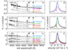 |
Fig. 8. Comparison of SN 2020pvb spectra before (a), around (b), and after (c) the maximum peak. We also include those of SNe 1994W, 2005cl, 2009kn, and 2011ht at similar epochs. The Hα profiles are enlarged on the right of each panel and shifted to the peak ((d), (e), and (f)). The Hα profiles of each SN match the colours of their label on the left. All spectra have been corrected for their host-galaxy recessional velocities and extinctions (values adopted from the literature). |
We estimated the photospheric temperatures by fitting the spectral continuum and the SED obtained with broadband photometry with a blackbody function (see Pastorello et al. 2021 for a detailed description of the procedure). We consider them upper limits due to the possibility of a blue excess at wavelengths shorter than 5500A (see the previous paragraph). As shown in Fig. 9 (panel a), there is a small scatter in temperature during the SN 2020pvb temporal evolution, ranging from 9000 to 10 500 K. These temperatures are higher than the recombination temperature of H. SN 2011ht is also significantly hotter and shows a constant temperature during the plateau phase, but there is clear evolution before and after it. On the contrary, the blackbody radius of the photosphere estimated through the Stefan–Boltzmann law exhibits a slow evolution peaking at 12 × 1014 cm at ∼11 d before the B-band maximum light, and then decreases to about 8.4 × 1014 cm at 38.6 d (panel b of Fig. 9). We note that these radii estimates are approximate, owing to the assumptions made to derive the temperatures and the luminosities of SN 2020pvb. In particular, the derived temperatures are more likely lower-limit estimates since we have assumed blackbody spectra without taking into account effects such as the metal line blanketing and the emission and absorption features.
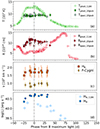 |
Fig. 9. Evolution of the best-fit blackbody temperatures (a), photospheric radius (b), FWHM and blueshift evolution for the whole profile and P Cygni Hα emission (c), and evolution of the total luminosity of Hα (d) of SN 2020pvb and SN 2011ht. The dot-dashed vertical line indicates the B-band maximum light of SN 2020pvb. |
The Balmer line profiles, particularly those of Hα, seem to consist of multiple components. We decomposed the Hα line profile at all epochs using a least-squares minimisation multi-component fit. Figure 10 presents the results of this fit at some representative epochs: rise (–24.3 d), around (1.7 d), and after (31.9 d), the B-band maximum. The profiles are reproduced using a single Lorentzian profile for all the spectra, including an additional Gaussian component in absorption when P Cygni features were visible (at phases > –21.3 d). The velocity estimates for the emission components (panel c of Fig. 9) are derived by measuring their FWHM, while those of the absorbing gas are estimated from the wavelengths of the P Cygni minima. The FWHM of the Hα emission (after correction for instrumental resolution14) remains nearly constant, with an average value of ∼1700 km s−1, while the absorption feature in the blue wing of Hα (shallow at late times) has a constant blueshift of ∼900 km s−1.
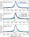 |
Fig. 10. Deblend of the Hα emission line of SN 2020pvb at –24.3, 1.7, and 31.9 d from the B-band maximum light. |
The observed Hα emission peak is blueshifted by about 100 km s−1 regarding the rest wavelength with a red tail extending to a higher velocity than the blue wing (see Fig. 10). This behaviour has been seen in other SN 1994W-like events and is explained by Dessart & Hillier (2005) as the results of multiple electron scattering for photons trapped in an optically thick emitting region.
The integrated luminosity of Hα (panel d of Fig. 9) evolves similarly as the broadband light curves. It shows a rise from LHα(–24.3 d) = 2.3 ± 0.4 × 1040 erg s−1 then remains roughly constant (since ∼10 days before the B-band peak) at ∼4.8 × 1040 erg s−1 during the plateau phase. SN 2020pvb has a substantially higher Hα luminosity than SN 2011ht (by a factor of ∼2) but it is fainter than SNe 1994W (see e.g. Fig. 8 of Mauerhan et al. 2013a). SN 2020pvb also shows an approximately constant luminosity evolution of Hα during the plateau phase. Similarly to SN 2011ht, we could expect a later decline. Unfortunately, our transient went behind the Sun, and we could not take any other measures.
5. Identification and nature of the progenitor candidate
We localised the SN 2020pvb position on the ACS/WFC images by performing differential astrometry between these and a V-band NOT+Alhambra Faint Object Spectrograph and Camera (ALFOSC) image taken on 2020 November 08, with a seeing of 0 8. We find SN 2020pvb position to correspond to the pixel coordinates 2389.80, 3372.46 on the F606W image with an associated RMS uncertainty
  (≈2.2 pixels).
We measured the brightness of the progenitor candidates using the DOLPHOT photometry package. We did not detect any source within an area of radius equal to the RMS uncertainty of the SN 2020pvb position. Instead, we identified several sources flagged as “object type = 1”, meaning they are likely stellar, at 5σ positional confidence within an area of radius 0 55. They are shown in Fig. 11. These sources are consistent with the position of SN 2020pvb, and therefore, the candidate progenitor of this SN could be one of them with a mag (in the Vega system) between 26.2 and 26.9 mag in F606W (corresponding to the brightest and faintest magnitude sources among those detected) or otherwise fainter than F606W = 26.9 mag.
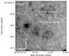 |
Fig. 11.
|


Correcting for the total extinction and distance assumed for SN 2020pvb (see Sect. 2), we find that the absolute magnitude of the progenitor was MF606W ≳ −8.7 mag. Not having colour information at the HST epoch, the progenitor initial mass is not well constrained and we can only set an upper limit of Mini ≲ 50 M⊙, depending on the bolometric correction (see Fig. 12). Therefore, the SN 2020pvb progenitor can be a low-mass luminous blue variable (these stars are usually suggested to be the progenitors of Type IIn SNe – Gal-Yam et al. 2007; Smartt et al. 2015) or a less massive star.
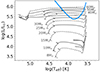 |
Fig. 12. Hertzsprung–Russell diagram showing the SN 2020pvb bolometric luminosity upper limit as a function of the effective temperature (solid blue line). The solid and dashed grey lines show single star evolutionary tracks from 8 to 60 M⊙ from the single star BPASS models (v2.2.1; Eldridge et al. 2017; Stanway & Eldridge 2018), assuming solar metallicity. |
6. Discussion and summary
6.1. Nature of SN 2020pvb
SN 2020pvb is a relatively bright (MB = −17.95 ± 0.30 mag) SN IIn with a plateau phase likely followed by a rapid decline. Persistent spectral signatures of interactions and a plateau-like photometric evolution classify SN 2020pvb as a SN IIn-P (Mauerhan et al. 2013a), akin to SNe 1994W, 2009kn, and 2011ht. These transients all have relatively high luminosities, are associated with low kinetic energies, and have low luminosities during the tail, implying a low 56Ni mass (e.g. Chugai 2016). We could consider a similar explosion scenario for SN 2020pvb, which would imply a low 56Ni mass. We roughly estimated a 56Ni mass ≤0.1 M⊙ from the first upper limit obtained after the solar conjunction (phase 157 d) and using the formula given by Hamuy (2003). We note that a 56Ni mass of 0.023 M⊙ was estimated for SN 2009kn (Kankare et al. 2015), the SN IIn-P with the most luminous known light curve tail (see the top panel of Fig. 3).
The observational characteristics of SN 2020pvb are so similar to those of SNe 1994W and 2011ht that these transients could have a similar physical interpretation. Figure 5 shows an abrupt luminosity decay after the SN 2020pvb plateau phase, with a late time flux upper limit of 1.5 × 1041 erg s−1 at phase 157 d and 8.8 × 1040 erg s−1 at phase 242 d. This could indicate that the 56Ni mass of SN 2020pvb is lower than 0.015 M⊙, the upper 56Ni mass limit estimated for SN 1994W (Sollerman et al. 1998).
SN 1994W-like SNe display similar strong Balmer lines with multiple components and a forest of narrow P Cygni lines of Fe II (see e.g. Fig. 8). SN 2020pvb shows shallow absorption features in the blue wing of Hα, Hβ, and Fe IIλ5018 with an average blueshift of ∼800–950 km s−1. These lines could arise from an outer, expanding shell lost by the progenitor star (e.g. SNe 1994aj and 1996L; Benetti et al. 1998, 1999, respectively). Considering the shell velocity as derived from the minima of the absorption (900 km s−1) and the inner shell radius close to that of the photosphere (8.5 × 1014 cm; we took the first value of the radius derived at phase –24.4 d), we estimate that the shell surrounding SN 2020pvb has15 an n ≫ 108 cm−3. However, the velocities measured in these absorption minima might not necessarily be associated with a steady wind in the outer, un-shocked shell, but rather with the interaction region between a faster inner shell and a slower outer shell. This scenario was presented by Dessart et al. (2016) and applied to SN 1994W. As described in this model, the fastest material of the inner shell, with some contribution from the accelerated outer shell material, is piled up in this region between the two shells, moving outwards at a constant velocity of about 900 km s−1. Another spectral characteristic of SN 2020pvb is its nearly flat Balmer decrement of Hα/Hβ ∼ 2, suggesting the contribution of radiative transitions or collisional thermalisation (Chugai et al. 2004).
6.2. Progenitor scenario
As for other similar transients, it is challenging to identify a unique progenitor scenario for SN 2020pvb. Here we discuss two simple possibilities:
Option A, a massive progenitor: Through HST images, we estimated the luminosity of the SN 2020pvb progenitor to be log(L/L⊙)≲5.4, which is consistent with a single star candidate with an initial mass Mini ≲ 50 M⊙. Recently, Matsumoto & Metzger (2022) modelled the optical precursor outburst detected from a sample of core-collapse SNe considering two scenarios: a single eruption or a continuous wind. Using their Eq. (30), we can estimate the wind mass-loss rate (Ṁ) in terms of observed precursor properties. With the previously derived progenitor values and considering 900 km s−1 to be the average wind velocity estimated from the narrow Hα P Cygni profile of SN 2020pvb (see Fig. 9), we obtain Ṁ = 6 × 10⁻⁵ M⊙ yr−1. This value is consistent with that of hyper-giant stars or luminous blue variable winds, particularly in outbursts (e.g. De Beck et al. 2010; Smith 2017b). Within the context of the massive progenitor scenario, that described by Heger et al. (2003), where a progenitor of around 40 M⊙ could generate a weak SN II, could even be valid. In this case, the ejecta interact with the possible mass lost by the star just before the explosion (for example, during the detected outburst). Then, once the interaction and recombination of the ejecta finishes, it cools down quickly because most of the 56Ni is swallowed by the black hole.
Option B, a moderate- to low-mass progenitor: The SN 2020pvb observables are also consistent with a low-mass progenitor surrounded by a dense CSM (Sollerman et al. 1998; Kankare et al. 2012; Mauerhan et al. 2013a; Chugai 2016), although it is unclear what the mechanism behind a precursor eruption of an 8–10 M⊙ progenitor could be.
As discussed in Sect. 5, PS1 detected an outburst in the w band of ∼–13.8 mag around 111 days before the B-band maximum light (∼50 days before the estimated explosion date). Interestingly, Fraser et al. (2013b) also reported a pre-SN eruption for SN 2011ht ∼6 months before its explosion at Mz = −11.8 mag. These events appear to confirm the Ofek et al. (2014b) and Strotjohann et al. (2021) findings that the outbursts of interacting SNe are frequent in the few months before SN explosions. We estimate a Lpre ≈ 9.6 × 1040 erg s−1 for the pre-SN outburst of SN 2020pvb. By directly multiplying this luminosity by its maximum possible duration, tpre = 48 d16, the radiated energy of the outburst is < 4 × 1047 erg, consistent with that observed for SN 2011ht (Fraser et al. 2013b)17. On the other hand, taking the gas velocity measured from the Fe IIλ5018 line (which is free from blending) as reference, its broad component (FWHM ∼ 800 km s−1) may be connected with the dense thin shell at the boundary between the SN and the circumstellar gas (Chugai 2001; Chugai & Danziger 2003). Therefore, assuming again 8.5 × 1014 cm as the shell radius, we estimate that this shell was ejected about four months before the explosion. This finding is roughly consistent with the date of the precursor outburst detected by the Pan-STARRS survey at the SN 2020pvb position.
Using Eqs. (25), (27), and (28) from Matsumoto & Metzger (2022) for a single eruption scenario based on the Popov formulae (Popov 1993), we can estimate an upper limit for the total ejected mass, Mshell, the outer CSM radius, Rshell, and the density profile of the precursor outburst, ρshell. Assuming a vej (velocity of the outburst ejecta) of 900 km s−1 (the shell velocity derived from the minima of the Hα absorption), Lpl = Lpre ≈ 9.6 × 1040 erg s−1 as the precursor luminosity, and tpl = tpre = 48 d the total duration time before the SN explosion, we obtain Mshell ≤ 0.3 M⊙, Rshell > 4 × 1014 cm, and ρshell < 2.5 × 10⁻¹² g cm−3.
Both Chugai et al. (2004) and Dessart et al. (2009) modelled the observables of SN 1994W, the prototype of this transient family, finding a need for a contribution from the interaction of the SN ejecta with a dense expanded circumstellar envelope. Another prototypical object of this class is SN 2011ht, which is observationally similar to SN 2020pvb; however, very early spectra are not available for the latter. The earliest spectrum of SN 2011ht showed a continuum temperature of ∼7000 K and narrow absorption lines (see Fig. 17 in Pastorello et al. 2019). To explain the unusual early spectrum and the slow photometric evolution, Roming et al. (2012) suggested that SN 2011ht exploded in a discontinuous CSM, with the bulk of the CSM located relatively far away. In this scenario, the ejecta–CSM interaction would be somewhat delayed. Given the similarity between the two SNe, we cannot rule out a similar scenario for SN 2020pvb. Some time later, Chugai (2016) claimed that the light curves and the low expansion velocity of SN 2011ht are consistent with a low-energy explosion (< 1050 erg) and a low ejecta mass (≲2 M⊙) interacting with a circumstellar envelope of 6–8 M⊙ and radius ∼2 × 1014 cm. The flat light curves suggest that the circumstellar interaction started soon after the explosion, with the CSM ejected shortly before the core collapse. In the same context of a moderate- to low-mass progenitor, Li & Morozova (2022) elaborate a somewhat different scenario as an explanation for the IIn-P sub-class: a 10 M⊙ red supergiant progenitor that had a precursor outburst of ∼1046 erg some months before it exploded (with a final energy of the order of 1051 erg). Single outbursts could be caused by a temporarily concentrated injection of energy, probably due to dynamical instabilities of nuclear-burning origin deep within the star, which generates a shock wave that propagates radially outwards and detaches a part of the stellar envelope (e.g. Dessart et al. 2010; Kuriyama & Shigeyama 2020; Matsumoto & Metzger 2022). They can also be responsible for outburst ejecta masses ≲0.27 M⊙ and a vej of 900 km s−1 (Matsumoto & Metzger 2022). Another possible cause of such violent ejections is explosive flashes of degenerate neon in < 8 M⊙ progenitors that are expected months to a few years before the SN explosion and can eject part of the hydrogen envelope with velocities of a few hundred km s−1 (Woosley et al. 2002; Fraser et al. 2013a). However, such flashes have not been reproduced by more recent models (Umeda et al. 2012; Chugai 2016).
Several authors also suggest an alternative scenario: a low-energy electron capture explosion (ECSN) of a super-AGB star with strong CSM interaction (e.g. Mauerhan et al. 2013a; Smith 2013; however, see also Li & Morozova 2022). Kozyreva et al. (2021) presented the light curves for an explosion of a super-AGB model with an initial zero-age main-sequence mass of 8.8 M⊙ that exploded as an ECSN (Stockinger et al. 2020). The default explosion of this model does not match SN 2020pvb. Therefore, we used a modified model that scales up the density of the SN ejecta. The resulting model has an ejecta mass of 0.4 M⊙, which corresponds to the same evolutionary model with a truncated radius of 400 R⊙. As suggested in Kozyreva et al. (2021), the truncated model imitates the effect of binarity. We surrounded the modified model with a wind-like CSM (i.e. with a CSM density ρCSM ∼ r−2) and ran simulations with the hydrodynamics radiative transfer code STELLA (Blinnikov & Bartunov 1993; Blinnikov et al. 2006). For the best-fit models, the total mass of the CSM is 2.2 M⊙ and 2.9 M⊙ for the e88W1 and e88W2 models, respectively, and the CSM radius is 1.5 × 1015 cm (see Fig. A.2). The luminosity and the shape of the main peak of the modelled light curves match the SN 2020pvb light curves reasonably well, although the synthetic light curves decline faster after the peak.
We stress that we cannot confidently rule out any of the progenitor scenarios presented here. In recent years, several interacting SNe with precursor events have been discovered (e.g. Ofek et al. 2014b; Jacobson-Galán et al. 2022). These transients highlight a gap in our current understanding of the final stages of a star’s life, as the conditions responsible for these eruptions are unclear. With continued attention to these precursor events, and the progenitors themselves, we will better understand how massive stars behave shortly before their death.
SN 2020pvb is also known as ATLAS20zmy, PS20gas, and ZTF20acghodf.
NED, the NASA/IPAC Extragalactic Database. It is funded by the National Aeronautics and Space Administration and operated by the California Institute of Technology; http://nedwww.ipac.caltech.edu/
Root-mean-squared (RMS) uncertainty.
ESO Faint Object Spectrograph and Camera. https://www.eso.org/sci/facilities/lasilla/instruments/efosc.html
A NIR spectrum was also obtained with the Especrografo Multiobjeto Infra-Rojo (EMIR) at the Gran Telescopio CANARIAS (GTC). However, this spectrum has a low S/N and lacks any obvious SN flux.
The spectra will be made public via the Weizmann Interactive Supernova Data Repository (WISeREP; Yaron & Gal-Yam 2012).
FOSCGUI is a graphic user interface aimed at extracting SN spectroscopy and photometry obtained with FOSC-like instruments. It was developed by E. Cappellaro. A package description can be found at http://sngroup.oapd.inaf.it/foscgui.html
We first corrected the measured FWHM for the spectral resolution ( ) and then computed the velocity (v = (width/λ0)×c).
We approximate the shell density, in terms of the hydrogen concentration for a normal abundance, as  , where v3 is the shell velocity in units of 103 km s−1, and r15 is the shell radius in units of 1015 cm.
Since the SN 2020pvb’s precursor was detected on just a single day, and there are Pan-STARRS survey non-detections both 24 days before and after the outburst, we assumed tpre = 48 d and assessed it as an upper limit. We want to note that the ATLAS survey had non-detections only five days before the outburst and also three days later. This would make a tpre of about eight days, reducing the radiated energy and the other estimated outburst parameters by about 17%. However, since the ATLAS survey’s non-detections are shallower than those obtained from the Pan-STARRS survey, we still consider the limit estimations from tpre = 48 d to be more robust.
See also Pastorello et al. (2019) who argue that the outburst of SN 2011ht was the outcome of a merger based on the similarities of its shape and duration of the light curve with that of luminous red novae.
Acknowledgments
N.E.R. thanks T. Matsumoto for useful discussions. We thank the staff at the different observatories for performing the observations. N.E.R., S.B., E.C., A.P., A.R., G.V. acknowledge support from the PRIN-INAF 2022, “Shedding light on the nature of gap transients: from the observations to the models”. S.J.B. would like to thank their support from Science Foundation Ireland and the Royal Society (RS-EA/3471). M.F. is supported by a Royal Society – Science Foundation Ireland University Research Fellowship. M.G. is supported by the EU Horizon 2020 research and innovation programme under grant agreement No. 101004719. N.I. was partially supported by Polish NCN DAINA grant No. 2017/27/L/ST9/03221. S.M. was funded by the Research Council of Finland project 350458. S.M. acknowledges support from the Magnus Ehrnrooth Foundation and the Vilho, Yrjö, and Kalle Väisälä Foundation. T.E.M.B. acknowledges financial support from the Spanish Ministerio de Ciencia e Innovación (MCIN), the Agencia Estatal de Investigación (AEI) 10.13039/501100011033 under the PID2020-115253GA-I00 HOSTFLOWS project, from Centro Superior de Investigaciones Científicas (CSIC) under the PIE project 20215AT016 and the I-LINK 2021 LINKA20409, and the program Unidad de Excelencia María de Maeztu CEX2020-001058-M. M.N. is supported by the European Research Council (ERC) under the European Union’s Horizon 2020 research and innovation programme (grant agreement No. 948381) and by a Fellowship from the Alan Turing Institute. Support for G.P. is provided by the Ministry of Economy, Development, and Tourism’s Millennium Science Initiative through grant IC120009, awarded to The Millennium Institute of Astrophysics (MAS). T.M.R. acknowledges the financial support of the Vilho, Yrjö and Kalle Väisälä Foundation of the Finnish academy of Science and Letters. S.J.S. is funded through STFC grant ST/T000198/1 L.T. acknowledges support from MIUR (PRIN 2017 grant 20179ZF5KS). Y.-Z. Cai is supported by the National Natural Science Foundation of China (NSFC, Grant No. 12303054) and the International Centre of Supernovae, Yunnan Key Laboratory (No. 202302AN360001). C.P.G. acknowledges financial support from the Secretary of Universities and Research (Government of Catalonia) and by the Horizon 2020 Research and Innovation Programme of the European Union under the Marie Skłodowska-Curie and the Beatriu de Pinós 2021 BP 00168 programme, from the Spanish Ministerio de Ciencia e Innovación (MCIN) and the Agencia Estatal de Investigación (AEI) 10.13039/501100011033 under the PID2020-115253GA-I00 HOSTFLOWS project, and the program Unidad de Excelencia María de Maeztu CEX2020-001058-M. This work made use of v2.2.1 of the Binary Population and Spectral Synthesis (BPASS) models as last described in Eldridge et al. (2017), Stanway & Eldridge (2018). This work was funded by ANID, Millennium Science Initiative, ICN12_009. This work makes use of observations from the Las Cumbres Observatory global telescope network. This work is based on observations made with the Nordic Optical Telescope, owned in collaboration by the University of Turku and Aarhus University, and operated jointly by Aarhus University, the University of Turku and the University of Oslo, representing Denmark, Finland and Norway, the University of Iceland and Stockholm University at the Observatorio del Roque de los Muchachos, La Palma, Spain, of the Instituto de Astrofisica de Canarias; ALFOSC, which is provided by the Instituto de Astrofisica de Andalucia (IAA) under a joint agreement with the University of Copenhagen and NOT; the Gran Telescopio Canarias (GTC), installed in the Spanish Observatorio del Roque de los Muchachos of the Instituto de Astrofísica de Canarias, in the island of La Palma; the Liverpool Telescope operated on the island of La Palma by Liverpool John Moores University in the Spanish Observatorio del Roque de los Muchachos of the Instituto de Astrofisica de Canarias with financial support from the UK Science and Technology Facilities Council; the Italian Telescopio Nazionale Galileo (TNG) operated the island of La Palma by the Fundación Galileo Galilei of the INAF (Istituto Nazionale di Astrofisica) at the Spanish Observatorio del Roque de los Muchachos of the Instituto de Astrofísica de Canarias; the STELLA robotic telescopes in Tenerife, an Leibniz-Institute for Astrophysics Potsdam (AIP) facility jointly operated by AIP and Instituto de Astrofísica de Canarias. Observations from the NOT were obtained through the NUTS2 collaboration which is supported in part by the Instrument Centre for Danish Astrophysics (IDA). We acknowledge funding to support our NOT observations from the Finnish Centre for Astronomy with ESO (FINCA), University of Turku, Finland (Academy of Finland grant nr 306531). Based on observations collected at the European Southern Observatory under ESO programmes ID 1103.D-0328 and 106.216C, as part of ePESSTO+ (the advanced Public ESO Spectroscopic Survey for Transient Objects Survey; PI: Inserra). LCO data have been obtained via an OPTICON proposals (IDs: SUPA2020B-002 and OPTICON 20B/003). The OPTICON project has received funding from the European Union’s Horizon 2020 research and innovation programme under grant no. 730890 Pan-STARRS is a project of the Institute for Astronomy of the University of Hawaii, and is supported by the NASA SSO Near Earth Observation Program under grants 80NSSC18K0971, NNX14AM74G, NNX12AR65G, NNX13AQ47G, NNX08AR22G, 80NSSC21K1572 and by the State of Hawaii. The Pan-STARRS data are processed at Queen’s University Belfast enabled through the STFC grants ST/P000312/1 and ST/T000198/1. This work has made use of data from the Asteroid Terrestrial-impact Last Alert System (ATLAS) project. The Asteroid Terrestrial-impact Last Alert System (ATLAS) project is primarily funded to search for near earth asteroids through NASA grants NN12AR55G, 80NSSC18K0284, and 80NSSC18K1575; by products of the NEO search include images and catalogs from the survey area. This work was partially funded by Kepler/K2 grant J1944/80NSSC19K0112 and HST GO-15889, and STFC grants ST/T000198/1 and ST/S006109/1. The ATLAS science products have been made possible through the contributions of the University of Hawaii Institute for Astronomy, the Queen’s University Belfast, the Space Telescope Science Institute, the South African Astronomical Observatory, and The Millennium Institute of Astrophysics (MAS), Chile. The ZTF forced-photometry service was funded under the Heising-Simons Foundation grant #12540303 (PI: Graham). This work makes use of observations from Neil Gehrels Swift Observatory (UVOT) and public data from the GALEX data archive.
References
- Artigau, E., Doyon, R., Vallee, P., Riopel, M., & Nadeau, D. 2004, in Ground-based Instrumentation for Astronomy, eds. A. F. M. Moorwood, & M. Iye, Proc. SPIE, 5492, 1479 [NASA ADS] [CrossRef] [Google Scholar]
- Benetti, S., Cappellaro, E., Danziger, I. J., et al. 1998, MNRAS, 294, 448 [NASA ADS] [CrossRef] [Google Scholar]
- Benetti, S., Turatto, M., Cappellaro, E., Danziger, I. J., & Mazzali, P. A. 1999, MNRAS, 305, 811 [NASA ADS] [CrossRef] [Google Scholar]
- Blanton, M. R., & Roweis, S. 2007, AJ, 133, 734 [NASA ADS] [CrossRef] [Google Scholar]
- Blinnikov, S. I., & Bartunov, O. S. 1993, A&A, 273, 106 [NASA ADS] [Google Scholar]
- Blinnikov, S. I., Röpke, F. K., Sorokina, E. I., et al. 2006, A&A, 453, 229 [NASA ADS] [CrossRef] [EDP Sciences] [Google Scholar]
- Brennan, S. J., & Fraser, M. 2022, A&A, 667, A62 [NASA ADS] [CrossRef] [EDP Sciences] [Google Scholar]
- Bruch, R. J., Gal-Yam, A., Schulze, S., et al. 2021, ApJ, 912, 46 [NASA ADS] [CrossRef] [Google Scholar]
- Cardelli, J. A., Clayton, G. C., & Mathis, J. S. 1989, ApJ, 345, 245 [Google Scholar]
- Chambers, K. C., Magnier, E. A., Metcalfe, N., et al. 2016, arXiv e-prints [arXiv:1612.05560] [Google Scholar]
- Chambers, K. C., Boer, T. D., Bulger, J., et al. 2020, TNSTR, 2020, 1 [Google Scholar]
- Chevalier, R. A., & Fransson, C. 1994, ApJ, 420, 268 [NASA ADS] [CrossRef] [Google Scholar]
- Chu, Y.-H., Gruendl, R. A., Stockdale, C. J., et al. 2004, AJ, 127, 2850 [NASA ADS] [CrossRef] [Google Scholar]
- Chugai, N. N. 2001, MNRAS, 326, 1448 [NASA ADS] [CrossRef] [Google Scholar]
- Chugai, N. N. 2016, Astron. Lett., 42, 82 [NASA ADS] [CrossRef] [Google Scholar]
- Chugai, N. N., & Danziger, I. J. 2003, Astron. Lett., 29, 649 [NASA ADS] [CrossRef] [Google Scholar]
- Chugai, N. N., Blinnikov, S. I., Cumming, R. J., et al. 2004, MNRAS, 352, 1213 [NASA ADS] [CrossRef] [Google Scholar]
- Cumming, R. J., & Lundqvist, P. 1997, Stellar Ecology: Advances in Stellar Evolution, 297 [Google Scholar]
- De Beck, E., Decin, L., de Koter, A., et al. 2010, A&A, 523, A18 [NASA ADS] [CrossRef] [EDP Sciences] [Google Scholar]
- Dessart, L., & Hillier, D. J. 2005, A&A, 437, 667 [NASA ADS] [CrossRef] [EDP Sciences] [Google Scholar]
- Dessart, L., Hillier, D. J., Gezari, S., Basa, S., & Matheson, T. 2009, MNRAS, 394, 21 [NASA ADS] [CrossRef] [Google Scholar]
- Dessart, L., Livne, E., & Waldman, R. 2010, MNRAS, 405, 2113 [NASA ADS] [Google Scholar]
- Dessart, L., Hillier, D. J., Audit, E., Livne, E., & Waldman, R. 2016, MNRAS, 458, 2094 [Google Scholar]
- de Vaucouleurs, G., de Vaucouleurs, A., Corwin, H. G., Jr., et al. 1991, Third Reference Catalogue of Bright Galaxies (New York: Springer), 2091 [Google Scholar]
- Dolphin, A. E. 2000, PASP, 112, 1383 [Google Scholar]
- Dolphin, A. 2016, Astrophysics Source Code Library [record ascl:1608.013] [Google Scholar]
- Eldridge, J. J., Stanway, E. R., Xiao, L., et al. 2017, PASA, 34, e058 [Google Scholar]
- Elias-Rosa, N. 2007, in The Multicolored Landscape of Compact Objects and Their Explosive Origins, eds. T. di Salvo, G. L. Israel, L. Piersant, et al., AIP Conf. Ser., 924, 395 [NASA ADS] [Google Scholar]
- Elias-Rosa, N., Benetti, S., Cappellaro, E., et al. 2006, MNRAS, 369, 1880 [CrossRef] [Google Scholar]
- Elias-Rosa, N., Pastorello, A., Benetti, S., et al. 2016, MNRAS, 463, 3894 [NASA ADS] [CrossRef] [Google Scholar]
- Elias-Rosa, N., Van Dyk, S. D., Benetti, S., et al. 2018, ApJ, 860, 68 [NASA ADS] [CrossRef] [Google Scholar]
- Fan, H., Hobbs, L. M., Dahlstrom, J. A., et al. 2019, ApJ, 878, 151 [NASA ADS] [CrossRef] [Google Scholar]
- Fraser, M. 2020, R. Soc. Open Sci., 7, 200467 [NASA ADS] [CrossRef] [Google Scholar]
- Fraser, M., Inserra, C., Jerkstrand, A., et al. 2013a, MNRAS, 433, 1312 [NASA ADS] [CrossRef] [Google Scholar]
- Fraser, M., Magee, M., Kotak, R., et al. 2013b, ApJ, 779, L8 [NASA ADS] [CrossRef] [Google Scholar]
- Gal-Yam, A., Leonard, D. C., Fox, D. B., et al. 2007, ApJ, 656, 372 [NASA ADS] [CrossRef] [Google Scholar]
- Gehrels, N., Chincarini, G., Giommi, P., et al. 2004, ApJ, 611, 1005 [Google Scholar]
- Hamuy, M. 2003, ApJ, 582, 905 [NASA ADS] [CrossRef] [Google Scholar]
- Heger, A., Fryer, C. L., Woosley, S. E., Langer, N., & Hartmann, D. H. 2003, ApJ, 591, 288 [CrossRef] [Google Scholar]
- Herbig, G. H. 1993, ApJ, 407, 142 [CrossRef] [Google Scholar]
- Herbig, G. H. 1995, ARA&A, 33, 19 [Google Scholar]
- Humphreys, R. M., Davidson, K., Jones, T. J., et al. 2012, ApJ, 760, 93 [NASA ADS] [CrossRef] [Google Scholar]
- Jacobson-Galán, W. V., Dessart, L., Jones, D. O., et al. 2022, ApJ, 924, 15 [CrossRef] [Google Scholar]
- Jester, S., Schneider, D. P., Richards, G. T., et al. 2005, AJ, 130, 873 [Google Scholar]
- Kankare, E., Ergon, M., Bufano, F., et al. 2012, MNRAS, 424, 855 [NASA ADS] [CrossRef] [Google Scholar]
- Kankare, E., Kotak, R., Pastorello, A., et al. 2015, A&A, 581, L4 [NASA ADS] [CrossRef] [EDP Sciences] [Google Scholar]
- Khazov, D., Yaron, O., Gal-Yam, A., et al. 2016, ApJ, 818, 3 [CrossRef] [Google Scholar]
- Kiewe, M., Gal-Yam, A., Arcavi, I., et al. 2012, ApJ, 744, 10 [NASA ADS] [CrossRef] [Google Scholar]
- Kozyreva, A., Baklanov, P., Jones, S., Stockinger, G., & Janka, H.-T. 2021, MNRAS, 503, 797 [NASA ADS] [CrossRef] [Google Scholar]
- Kuriyama, N., & Shigeyama, T. 2020, A&A, 635, A127 [NASA ADS] [CrossRef] [EDP Sciences] [Google Scholar]
- Li, C., & Morozova, V. 2022, MNRAS, 515, 3597 [CrossRef] [Google Scholar]
- Magnier, E. A., Schlafly, E. F., Finkbeiner, D. P., et al. 2020, ApJS, 251, 6 [NASA ADS] [CrossRef] [Google Scholar]
- Maguire, K., Di Carlo, E., Smartt, S. J., et al. 2010, MNRAS, 404, 981 [NASA ADS] [CrossRef] [Google Scholar]
- Margutti, R., Milisavljevic, D., Soderberg, A. M., et al. 2014, ApJ, 780, 21 [Google Scholar]
- Martin, D. C., Fanson, J., Schiminovich, D., et al. 2005, ApJ, 619, L1 [Google Scholar]
- Masci, F. J., Laher, R. R., Rusholme, B., et al. 2019, PASP, 131, 018003 [Google Scholar]
- Matsumoto, T., & Metzger, B. D. 2022, ApJ, 936, 114 [CrossRef] [Google Scholar]
- Mauerhan, J. C., Smith, N., Silverman, J. M., et al. 2013a, MNRAS, 431, 2599 [Google Scholar]
- Mauerhan, J. C., Smith, N., Filippenko, A. V., et al. 2013b, MNRAS, 430, 1801 [NASA ADS] [CrossRef] [Google Scholar]
- Moriya, T. J., & Maeda, K. 2014, ApJ, 790, L16 [NASA ADS] [CrossRef] [Google Scholar]
- Mould, J. R., Huchra, J. P., Freedman, W. L., et al. 2000, ApJ, 529, 786 [Google Scholar]
- Nyholm, A., Sollerman, J., Tartaglia, L., et al. 2020, A&A, 637, A73 [NASA ADS] [CrossRef] [EDP Sciences] [Google Scholar]
- Ofek, E. O., Sullivan, M., Cenko, S. B., et al. 2013, Nature, 494, 65 [CrossRef] [Google Scholar]
- Ofek, E. O., Zoglauer, A., Boggs, S. E., et al. 2014a, ApJ, 781, 42 [CrossRef] [Google Scholar]
- Ofek, E. O., Sullivan, M., Shaviv, N. J., et al. 2014b, ApJ, 789, 104 [NASA ADS] [CrossRef] [Google Scholar]
- Ofek, E. O., Cenko, S. B., Shaviv, N. J., et al. 2016, ApJ, 824, 6 [CrossRef] [Google Scholar]
- Pastorello, A., Kochanek, C. S., Fraser, M., et al. 2018, MNRAS, 474, 197 [NASA ADS] [CrossRef] [Google Scholar]
- Pastorello, A., Mason, E., Taubenberger, S., et al. 2019, A&A, 630, A75 [NASA ADS] [CrossRef] [EDP Sciences] [Google Scholar]
- Pastorello, A., Fraser, M., Valerin, G., et al. 2021, A&A, 646, A119 [EDP Sciences] [Google Scholar]
- Perley, D. A., Taggart, K., Dahiwale, A., & Fremling, C. 2020, TNS Classif. Rep., 2020, 1 [Google Scholar]
- Phillips, M. M., Simon, J. D., Morrell, N., et al. 2013, ApJ, 779, 38 [NASA ADS] [CrossRef] [Google Scholar]
- Popov, D. V. 1993, ApJ, 414, 712 [NASA ADS] [CrossRef] [Google Scholar]
- Poznanski, D., Ganeshalingam, M., Silverman, J. M., & Filippenko, A. V. 2011, MNRAS, 415, L81 [NASA ADS] [CrossRef] [Google Scholar]
- Reguitti, A., Pastorello, A., Pignata, G., et al. 2019, MNRAS, 482, 2750 [NASA ADS] [Google Scholar]
- Riess, A. G., Casertano, S., Yuan, W., et al. 2021, ApJ, 908, L6 [NASA ADS] [CrossRef] [Google Scholar]
- Roming, P. W. A., Pritchard, T. A., Prieto, J. L., et al. 2012, ApJ, 751, 92 [NASA ADS] [CrossRef] [Google Scholar]
- Schlafly, E. F., & Finkbeiner, D. P. 2011, ApJ, 737, 103 [Google Scholar]
- Schlegel, E. M. 1990, MNRAS, 244, 269 [NASA ADS] [Google Scholar]
- Smartt, S. J., Valenti, S., Fraser, M., et al. 2015, A&A, 579, A40 [NASA ADS] [CrossRef] [EDP Sciences] [Google Scholar]
- Smith, N. 2011, MNRAS, 415, 2020 [Google Scholar]
- Smith, N. 2013, MNRAS, 434, 102 [Google Scholar]
- Smith, N. 2017a, Philos. Trans. R. Soc. Lond. Ser. A, 375, 20160268 [NASA ADS] [Google Scholar]
- Smith, N. 2017b, in Handbook of Supernovae, eds. A. W. Alsabti, & P. Murdin, 403 [CrossRef] [Google Scholar]
- Smith, K. W., Smartt, S. J., Young, D. R., et al. 2020, PASP, 132, 085002 [Google Scholar]
- Sollerman, J., Cumming, R. J., & Lundqvist, P. 1998, ApJ, 493, 933 [NASA ADS] [CrossRef] [Google Scholar]
- Stanway, E. R., & Eldridge, J. J. 2018, MNRAS, 479, 75 [NASA ADS] [CrossRef] [Google Scholar]
- Stockinger, G., Janka, H. T., Kresse, D., et al. 2020, MNRAS, 496, 2039 [Google Scholar]
- Strotjohann, N. L., Ofek, E. O., Gal-Yam, A., et al. 2021, ApJ, 907, 99 [NASA ADS] [CrossRef] [Google Scholar]
- Taddia, F., Stritzinger, M. D., Sollerman, J., et al. 2013, A&A, 555, A10 [NASA ADS] [CrossRef] [EDP Sciences] [Google Scholar]
- Tartaglia, L., Pastorello, A., Sullivan, M., et al. 2016, MNRAS, 459, 1039 [NASA ADS] [CrossRef] [Google Scholar]
- Tartaglia, L., Sand, D. J., Groh, J. H., et al. 2021, ApJ, 907, 52 [NASA ADS] [CrossRef] [Google Scholar]
- Thöne, C. C., de Ugarte Postigo, A., Leloudas, G., et al. 2017, A&A, 599, A129 [NASA ADS] [CrossRef] [EDP Sciences] [Google Scholar]
- Tonry, J. L., Denneau, L., Heinze, A. N., et al. 2018, PASP, 130, 064505 [Google Scholar]
- Tsvetkov, D. Y. 1995, Inf. Bull. Var. Stars, 4253, 1 [NASA ADS] [Google Scholar]
- Umeda, H., Yoshida, T., & Takahashi, K. 2012, Prog. Theor. Exp. Phys., 2012, 01A302 [CrossRef] [Google Scholar]
- Vink, J. S. 2008, Proc. Int. Astron. Union, 4, 271 [NASA ADS] [CrossRef] [Google Scholar]
- Vladilo, G., Crivellari, L., Molaro, P., & Beckman, J. E. 1987, A&A, 182, L59 [NASA ADS] [Google Scholar]
- Weis, K. 2001, Rev. Mod. Astron., 14, 261 [NASA ADS] [Google Scholar]
- Woosley, S. E., Heger, A., & Weaver, T. A. 2002, Rev. Mod. Phys., 74, 1015 [NASA ADS] [CrossRef] [Google Scholar]
- Yaron, O., & Gal-Yam, A. 2012, PASP, 124, 668 [Google Scholar]
Appendix A: Additional figures of SN 2020pvb
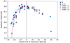 |
Fig. A.1. Bluest-band light curves of SN 2020pvb shifted at its maximum light. The solid line is the best-fit polynomial of the light curve rise. The dot-dashed vertical line indicates the B-band maximum light. |
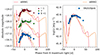 |
Fig. A.2. Absolute BVr(left) and uUBVri pseudo-bolometric (right) light curves of SN 2020pvb, compared with those for the ECSN model from Kozyreva et al. (2021) surrounded by a wind-like CSM. |
Appendix B: Tables of photometry and spectroscopy of SN 2020pvb
Basic information about the telescopes and instruments used (in alphabetical order by key).
UBV (VEGA MAG) photometry of SN 2020pvb.
ugriz (AB MAG) photometry of SN 2020pvb.
JHK (VEGA MAG) photometry of SN 2020pvb.
PS1 w-band (AB MAG) photometry of SN 2020pvb.
Cyan and orange (AB MAG) photometry of SN 2020pvb.
Log of spectroscopic observations of SN 2020pvb.
UVW2, UVM2, and UVW1 (VEGA MAG) photometry of SN 2020pvb.
All Tables
Basic information about the telescopes and instruments used (in alphabetical order by key).
All Figures
|
Fig. 1. NOT+ALFOSC image of the SN 2020pvb field in the r band obtained on 2020 October 15. The position of the SN is indicated with a circle, and a close-up of the area around the SN is shown in the upper-right inset. |
| In the text | |
|
Fig. 2. Light curves of SN 2020pvb. Top: UV-optical-NIR light curves of SN 2020pvb. Upper limits are indicated by empty symbols with arrows. Bottom: Historical light curves of SN 2020pvb. Upper limits are indicated by empty symbols with arrows. The light curves have been shifted for clarity by the amounts indicated in the legend. The right insert is a 27″ × 27″ zoomed-in view of the transient position in the difference image (observation minus reference image) taken on 2020 July 18 in the PS1 w band. The precursor outburst is detected at a greater than 5-sigma significance. |
| In the text | |
|
Fig. 3. Absolute B light curve of SN 2020pvb, shown together with those of SNe 1994W, 2005cl, 2009kn, 2011ht, and the Type IIP SN 2004et. Upper limits are indicated by vertical arrows. The dot-dashed vertical line indicates the B-band maximum light. The uncertainties for most data points are smaller than the plotted symbols. |
| In the text | |
|
Fig. 4. Intrinsic colour evolution of SN 2020pvb, compared with those of SNe 1994W, 2005cl, 2009kn, 2011ht, and the Type IIP SN 2004et. The dot-dashed vertical line indicates the B-band maximum light of SN 2020pvb. |
| In the text | |
|
Fig. 5. Pseudo-bolometric light curve of SN 2020pvb obtained by integrating optical and NIR bands, compared with those of SNe 1994W, 2005cl, 2009kn, 2011ht, and the Type IIP SN 2004et. The UV-optical-NIR pseudo-bolometric light curve of SN 2020pvb is also included. The dot-dashed vertical line indicates the B-band maximum light of SN 2020pvb. |
| In the text | |
|
Fig. 6. Spectral sequence of SN 2020pvb extending from –24.3 d to 31.9 d from maximum light. All spectra have been corrected by redshift. The shaded wavelength regions indicate areas of strong telluric absorption, which has been removed when possible. The locations of the most prominent spectral features are also indicated. |
| In the text | |
|
Fig. 7. Superposition of the 2020 October 15.88 UTC (–21.3 d, solid grey line) and 2020 December 08.03 UTC (31.9 d, dotted black line) spectra of SN 2020pvb. The insert is a zoomed-in view of the absorptions between 6300 and 6400 Å. The most prominent spectral features are indicated. |
| In the text | |
|
Fig. 8. Comparison of SN 2020pvb spectra before (a), around (b), and after (c) the maximum peak. We also include those of SNe 1994W, 2005cl, 2009kn, and 2011ht at similar epochs. The Hα profiles are enlarged on the right of each panel and shifted to the peak ((d), (e), and (f)). The Hα profiles of each SN match the colours of their label on the left. All spectra have been corrected for their host-galaxy recessional velocities and extinctions (values adopted from the literature). |
| In the text | |
|
Fig. 9. Evolution of the best-fit blackbody temperatures (a), photospheric radius (b), FWHM and blueshift evolution for the whole profile and P Cygni Hα emission (c), and evolution of the total luminosity of Hα (d) of SN 2020pvb and SN 2011ht. The dot-dashed vertical line indicates the B-band maximum light of SN 2020pvb. |
| In the text | |
|
Fig. 10. Deblend of the Hα emission line of SN 2020pvb at –24.3, 1.7, and 31.9 d from the B-band maximum light. |
| In the text | |
|
Fig. 11.
|
| In the text | |
|
Fig. 12. Hertzsprung–Russell diagram showing the SN 2020pvb bolometric luminosity upper limit as a function of the effective temperature (solid blue line). The solid and dashed grey lines show single star evolutionary tracks from 8 to 60 M⊙ from the single star BPASS models (v2.2.1; Eldridge et al. 2017; Stanway & Eldridge 2018), assuming solar metallicity. |
| In the text | |
|
Fig. A.1. Bluest-band light curves of SN 2020pvb shifted at its maximum light. The solid line is the best-fit polynomial of the light curve rise. The dot-dashed vertical line indicates the B-band maximum light. |
| In the text | |
|
Fig. A.2. Absolute BVr(left) and uUBVri pseudo-bolometric (right) light curves of SN 2020pvb, compared with those for the ECSN model from Kozyreva et al. (2021) surrounded by a wind-like CSM. |
| In the text | |
Current usage metrics show cumulative count of Article Views (full-text article views including HTML views, PDF and ePub downloads, according to the available data) and Abstracts Views on Vision4Press platform.
Data correspond to usage on the plateform after 2015. The current usage metrics is available 48-96 hours after online publication and is updated daily on week days.
Initial download of the metrics may take a while.