| Issue |
A&A
Volume 686, June 2024
|
|
|---|---|---|
| Article Number | A306 | |
| Number of page(s) | 16 | |
| Section | Astronomical instrumentation | |
| DOI | https://doi.org/10.1051/0004-6361/202347885 | |
| Published online | 25 June 2024 | |
End-to-end simulations of exoplanet detection with multiplexed volume Bragg gratings
1
Leiden Observatory, Leiden University,
Niels Bohrweg 2,
2333 CA
Leiden,
The Netherlands
e-mail: This email address is being protected from spambots. You need JavaScript enabled to view it.
2
National Solar Observatory,
3665 Discovery Drive,
Boulder,
CO
80303,
USA
e-mail: This email address is being protected from spambots. You need JavaScript enabled to view it.
Received:
5
September
2023
Accepted:
26
March
2024
Abstract
Context. Direct imaging of exoplanets greatly enhances our ability to spectroscopically detect molecules in their atmospheres, but requires both excellent angular and spectral resolution. A highly promising approach uses multiplexed transmission gratings to achieve compressed sensing, but the published theoretical calculations are not realistic enough to determine whether the approach is feasible.
Aims. We aim to determine the performance of recovering exoplanet signals of an instrument with multiplexed volume Bragg gratings in a full, detailed numerical simulation, specifically examining any effects caused by multiplexing several gratings.
Methods. Our end-to-end simulation includes realistic stellar and planetary spectra, a closed-loop adaptive optics simulation, and rigorous coupled wave analysis to model the multiplexed gratings. We chose 20 passbands around expected methane absorption features that were optically combined using 20 gratings.
Results. We find that exoplanet signals can be recovered down to contrasts of 10−6−10−7, without the addition of a coronagraph. Multiplexing a larger number of gratings improves the deepest recovered contrast, if photon noise is the dominant noise source. When residuals from our simple post-processing approach are the largest noise source, a larger number of multiplexed gratings decreases the performance, due to the stacking of the PSFs at different wavelengths. This is an artifact of our data reduction approach.
Conclusions. We conclude that multiplexed Bragg gratings are a viable method to look for exoplanets with a compressed sensing approach, and additional gains may be made in post-processing.
Key words: instrumentation: high angular resolution / instrumentation: miscellaneous / instrumentation: spectrographs / methods: numerical / techniques: imaging spectroscopy
© The Authors 2024
 Open Access article, published by EDP Sciences, under the terms of the Creative Commons Attribution License (https://creativecommons.org/licenses/by/4.0), which permits unrestricted use, distribution, and reproduction in any medium, provided the original work is properly cited.
This article is published in open access under the Subscribe to Open model. This email address is being protected from spambots. You need JavaScript enabled to view it. to support open access publication.
1 Introduction
The spectral diversity between a star and its exoplanets greatly enhances the success of direct imaging for finding and characterizing exoplanets. The differences in the spectra are largely due to the differences in composition and temperature between a host star and its planets (see for example Snellen et al. 2015). Typically, exoplanets exhibit emission spectra containing molecular lines not found in the stellar spectrum. Integral field spectrographs such as the Spectrograph for INtegral Field Observations in the Near Infrared (SINFONI; Eisenhauer et al. 2003) or the Multi Unit Spectroscopic Explorer (MUSE; Bacon et al. 2010) can detect compounds on exoplanets, such as the result of Hoeijmakers et al. (2018), who found CO2 and H2O on β Pic b, or the discovery of PDS 70c by Haffert et al. (2019a) through its Hα emission.
While it is possible to infer the presence of a molecule from a single, bright spectral line (such as Hα), molecules with lower abundances and for colder exoplanets require the combination of light from several molecular lines. These lines must then be combined in post-processing into a single signal. The data cubes resulting from integral field instruments contain both spatial and spectral information that can typically be represented as a spectrum for each spatial element. These spectra can be cross-correlated with a (possibly Doppler-shifted) template spectrum of the desired molecule, thus reducing the measured spectrum to a number proportional to the abundance of a molecule (Snellen et al. 2010).
Integral field spectroscopy is a powerful way to directly image exoplanets; however, it requires both high-resolution spectra over a broad wavelength range and high spatial resolution. High-resolution spectra are required to properly resolve individual molecular lines, and high spatial resolution is necessary to resolve the star and the planet. The intrinsically three-dimensional data need to be transformed onto a two-dimensional detector. This leads to a trade-off between spectral bandwidth, spectral resolution, and spatial resolution. For a fixed number of detector pixels and spectral bandwidth, every pixel used to increase the spectral resolution cannot be used to increase the spatial resolution or field size, and vice versa. Current solutions sacrifice spectral resolution such as in the Spectro-Polarimetric High-contrast Exoplanet REsearch (SPHERE; Beuzit et al. 2019) and the Gemini Planet Imager (GPI; Macintosh et al. 2014) with a spectral resolution of R ~ 70, or limit their number of targets for more spectral resolution like the Optical System for Imaging and low-Intermediate-Resolution Integrated Spectroscopy (OSIRIS; Cepa et al. 2003). MUSE spreads the light out over multiple detectors, spreading the three-dimensional data over multiple two-dimensional detectors. This allows for both high spatial and spectral resolution, at the cost of a very large and complex instrument.
When looking for a specific molecule, we can sidestep this trade-off by noting that we do not need to record an entire spectrum: we only need to measure narrow passbands around spectral features of interest. Taking this approach even further, we can use correlations of spectra; for narrow absorption lines this corresponds approximately to a weighted summing over multiple spectral lines. This can be done in post-processing (Hoeijmakers et al. 2018), but can also be approximated by incoherently adding the light from these multiple passbands before detection. In the latter case, we do not need to measure individual lines at all, thereby greatly reducing the amount of detector space needed per spatial feature.
Haffert et al. (2019b) propose to use an acousto-optical tunable filter (AOTF) to create multiplexed volume Bragg gratings to stack molecular lines. Spectrometers based on AOTFs are widely used in science, for instance to measure trace gases like NO2 in the Earth’s atmosphere (Dekemper et al. 2016). They did not multiplex gratings, instead using the AOTF as a filter to take two separate images with different central grating wavelengths.
The simulations of Haffert et al. (2019b) use a simplified model of the Bragg gratings and the optical system. Our goal in this paper is two-fold: we want to expand on their model and create a code that fully simulates multiplexed Bragg gratings and that can function in an end-to-end high-contrast imaging simulation. We then wish to use this code to create a set of end-to-end simulations of a star and exoplanet. We will attempt to recover the exoplanet, and derive requirements for the optical system when using this novel device for exoplanet detection.
Our code for the multiplexed Bragg gratings is based on the rigorous coupled wave analysis (RCWA) description of multiplexed Bragg gratings by Moharam & Gaylord (1981). This code solves Maxwell’s equations for a plane wave propagating through the grating.
We use this code in an end-to-end simulation of a star with an exoplanet. We attempt to recover an exoplanet with a fully simulated emission spectrum from several different molecules and at separations of 1 to 4λ/D from its star. We attempt to detect the exoplanet without using any prior knowledge of its spectrum. We only rely on the absorption spectrum from CH4 to choose central wavelengths for the gratings. With this restriction we wish to determine 1) if we can still recover an exoplanet with our more realistic simulation; 2) what exoplanet contrasts can be achieved in ideal circumstances and when limited by shot noise; and 3) the effect of multiplexing more gratings on the limiting contrast. We also discuss several factors to consider when designing an instrument using multiplexed Bragg gratings, such as the beam size used in the instrument and the arrangement of a fiber array in our simulated optical setup.
We start by discussing the architecture of the end-to-end simulation code using hcipy (Por et al. 2018) in Sect. 2, starting with the optical layout (Sect. 2.1), implementation of an atmosphere corrected by an adaptive optics (AO) system (Sect. 2.2), and generating source spectra (Sect. 2.3). We discuss Bragg gratings and our implementation in Sect. 3, introducing Bragg grating properties and their advantages for compressed spec-troscopy in Sect. 3.1, the concept of multiplexing Bragg gratings in 3.2, and how Bragg gratings are typically implemented in Sect. 3.3. We follow with a description of the rigorous coupled wave analysis (RCWA) code written for our simulations in Sects. 3.4 and 3.5, and our approach for the data reduction in Sect. 4. We present the results of the end-to-end simulation in Sect. 5, showing the reduced data cube of a single simulation in Sect. 5.1, the effect of varying the number of gratings in Sect. 5.2, and contrast limits in Sect. 5.3. In Sect. 6 we discuss considerations when using multiplexed Bragg gratings to design an instrument, such as the required beam size on a grating and ways to reformat the fiber array to maximize the performance.
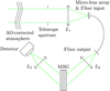 |
Fig. 1 Layout of the optical system in our simulations. The light starts in the upper left corner, being propagated to a fiber array. The output of the fiber array is passed through the set of multiplexed Bragg gratings and focused onto the detector. See the text in Sect. 2.1 for more details. |
2 Exoplanet integral field unit simulation
We simulated an instrument with the general layout of a fiber-fed integral field spectrograph (IFS) that uses multiplexed Bragg gratings as the main dispersive element. The multiplexed Bragg gratings are present in a single optic, but act as several transmission gratings at the same time. Each of these gratings has their own narrow passband (centered on spectral lines of a specific molecule) with a spectral width of ~1 nm and a tunable central wavelength of light being sent to the detector. The light from each grating overlaps with the light from the other gratings, giving us a set of optically stacked passbands on our detector for each fiber. The core concept of this instrument is stacking multiple passbands of interest for exoplanet detection.
2.1 Optical layout
The general layout for our optical setup in the simulation is shown in Fig. 1, with specific parameters shown in Table 1. Broadly speaking, the optical setup has two main parts: an ideal telescope with a turbulent atmosphere focusing light onto a fiber array, and the output of the fiber array being passed through a set of multiplexed Bragg gratings (MBG). Apart from using our own code for the MBG, we used hcipy (Por et al. 2018) with some custom additions to model the wavefronts and calculate their propagation through the various optical elements.
Incoming light passes through a phase screen from a simulated atmosphere corrected by adaptive optics (AO) (see Sect. 2.2). It is subsequently focused by an idealized telescope with a circular, unobstructed aperture. The focal plane is imaged again by a rectangular micro-lens array onto a single-mode fiber array, so every fiber sees a small square of the telescope PSF. The bottom panel in Fig. 2 shows our placement of the micro-lens and fiber array. We used single-mode fibers, both to reduce the computational complexity of the simulation, and to reduce the coupling of the first Airy ring into the fibers (cf. Por & Haffert 2020).
Following Por & Haffert (2020) we did not forward-propagate every wavefront through the telescope and then calculate the coupling to a fiber. Instead we back-propagated the Gaussian fiber modes through the telescope and calculated the coupling between a back-propagated fiber mode and an incoming wavefront. This required us to perform Fresnel and Fraunhofer propagations on wavefronts for every fiber mode (121 total) and every wavelength (2360 total), giving 2360 × 121 ≈ 2.9 × 10⁵ wavefronts to propagate. If we forward-propagated every wavelength (again 2360 total) we used and every atmospheric wavefront aberration (300 total), we would have ended up with around 2360 × 300 ≈ 7 × 10⁵ wavefronts to propagate. The advantages of the back-propagation approach therefore increase with the number of atmospheric wavefront realizations.
Our focus on exoplanet direct imaging implies a small field of view (FOV). Each fiber sees a 0″.18 by 0″.18 square, so the total FOV we consider with an 11 × 11 fiber array is a square with 2″ sides. We did not consider any light outside this FOV, though in principle this could be used to track a guide star. We wished to reach a high spectral resolution to resolve molecular lines. We therefore chose a passband of ~±100 km s−1 velocity offset for our gratings. Around 100 spectral data points per spaxel resulted in a spectral resolution of R ≈ 1.5 × 10⁵ for our MBG.
We used the flexibility of fibers to reformat the input configuration (see Sect. 6.2) and separate each fiber by a distance Dbeam. The light from each fiber is then collimated by a separate lens and passes through the MBG. The MBG diffracts part of the light to its first transmitted order and leaves the rest in its zeroth transmitted order (see Sect. 3.1). We discarded the light in the zeroth transmitted order in our simulation, but in an instrument this may be used for wavefront sensing or astrometry. The light from the first transmitted order is finally focused onto a detector. This creates an optically stacked spectrum for each fiber (see Sect. 3.2 and Fig. 5). An example spectrum for a single fiber can be seen in the top panel in Fig. 2. Because the fibers are well separated and separately focused, the different spectra on the detector do not overlap. We summed all pixels perpendicular to the dispersion direction to obtain a 1-dimensional spectrum for each fiber (also shown in Fig. 2). The full simulation produces a data cube similar to the output of an IFU, with two spatial dimensions and one spectral. We separately propagated the light from the star and exoplanet, using their mutual incoherence to calculate the final data cube as a weighted sum at the desired contrast. We also saved the result for each grating separately, providing us with a simple way to vary the number of multiplexed gratings. We did not include any optical errors such as alignment or surface errors for any of the optics in our optical model, as we want to focus on the inherent limitations of using multiplexed Bragg gratings, rather than any effects of imperfect optics.
Simulation parameters for the telescope, micro-lens array, fiber bundle, and the multiplexed Bragg gratings.
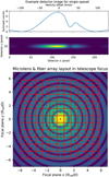 |
Fig. 2 Example detector output for a single spaxel and the layout of the micro-lens and input fiber array in the telescope focus. The top figure shows both the simulated detector image and that image summed along one axis. The top x-axis gives the velocity offset from the Bragg wavelength corresponding to the pixel values. The figure uses the data for a single spaxel with one multiplexed Bragg grating with Bragg wavelength 1.083 µm and the emission spectrum of the planet. The planet has an absorption feature between the 0 and 50 km s−1 velocity offsets. The bottom figure shows the boundaries of each micro-lens in the micro-lens array with red lines and the fiber positions behind the micro-lens array with red dots. The Airy pattern visible beneath is a perfect Airy pattern at wavelength λref to illustrate the rough position of each fiber. |
2.2 Atmospheric simulation
The parameters for the telescope, atmosphere, and AO can be found in Table 2. For simplicity and because of the large set of possible telescope shapes, we chose an unobscured circular aperture.
We used a model consisting of multiple frozen flow layers at different altitudes for the atmospheric simulation, excluding scintillation for simplicity. Every layer consists of Kolmogorov noise with separate  values and wind speeds. The wind speed per layer is kept fixed, but the wind direction per layer is randomized, so the total atmospheric phase is not a single frozen flow. The atmospheric noise is corrected by a square grid of Gaussian pokes as a simple model for a deformable mirror. We did not include a model for a wavefront sensor, only adding a small lag between the current atmospheric phase screen and the correction by the deformable mirror. This means that the corrected wave-front will be less noisy than otherwise expected. Together with neglecting any wavefront errors including surface errors in all optics, we therefore expect our contrast and limits on the signal-to-noise ratio (S/N) to be upper bounds. We used two time steps to generate a phase screen: one large step to reduce correlations between separate phase screens and a small step to implement the AO lag.
Parameters used in the telescope and atmospheric & adaptive optics simulation.
2.3 Source spectra
Initial tests for the simulation code were performed with absorption lines with idealized Gaussian profiles on a flat continuum. For the simulations presented here the stellar spectrum is taken from the BT-Settl stellar spectra library (Allard 2014). We chose a model with similar properties to HR8799 as found in Gray & Kaye (1999).
The planetary spectrum is generated using the petitRADTRANS software package (Mollière et al. 2019). The planet properties are based on the properties of HR8799c from Marois et al. (2008) and Wang et al. (2021). The species included in the emission spectrum calculation are H2O, CO, CH4, CO2, and K, with H2 and He included for Rayleigh scattering and continuum opacities. Table 3 shows parameters and values used in the petitRADTRANS simulation. We calculated the mass fractions for each species with the chemical equilibrium model included with petitRADTRANS, using the resulting values to calculate the emission spectrum. We linearly shifted the emission spectrum by 30 km s−1 to model the Doppler shift of the exoplanet with respect to the host star.
Each grating in the MBG has a small passband with a central wavelength and spectral width Δλ (see Sect. 3.1) of light that gets diffracted to the first transmitted order. The petitRADTRANS planetary spectrum simulation uses (up to) 20 of the most prominent absorption features of CH4 between 1 and 2 µm to determine the central wavelengths for each grating. For this line selection, we used the absorption spectrum for CH4 from the HITRAN database (Gordon et al. 2017). The biggest absorption features are determined by the general peak-finding algorithm of scipy (Virtanen et al. 2020). To ensure that the gratings can be modeled independently (see Sect. 3.5), we picked the central wavelengths of each grating such that there is at least 3ΔλB between each pair of central wavelengths (Fu et al. 1997), greedily choosing the highest peaks first.
Parameters used in the petitRADTRANS calculation of the planetary emission spectrum and selection of the BT-Settl stellar spectrum.
3 Bragg gratings
3.1 Basics
A Bragg grating functions as a transmission grating where the grating is created by a periodic modulation of the index of refraction in the bulk material, rather than a periodic surface structure. Incoming light is diffracted into various transmission orders, with the throughput per order depending on the grating spacing, incoming angle, and the grating thickness. An incoming wave satisfies the grating equation
 (1)
(1)
with λ the wavelength of the incoming light, n the average refractive index of the grating material, and σ the grating pitch, equivalent to the line spacing of a standard diffraction grating. A schematic of a Bragg grating setup can be seen in Fig. 3. Similar to an electromagnetic plane wave, we can assign a wave vector to the periodic modulation in refractive index. In our case this wave vector is parallel to the grating surface such that the grating acts as a transmission grating. If this wave vector is normal to the grating surface, the Bragg grating behaves similar to a thin-film stack. This is used in for example fiber Bragg gratings.
For gratings with thicknesses comparable to a wavelength d ~ λ, there is diffraction into various orders (Moharam & Gaylord 1981), but for thick gratings d >> λ we enter the Bragg regime, where transmission into all orders but the zeroth and first can be neglected. The diffraction efficiency (DE) of a diffraction order is the fraction of the input energy going into that diffraction order. When we refer to the DE without referencing a diffraction order, we mean the DE to the first transmitted order. For example, a DE of 100% means that all incoming light is diffracted into the first transmission order. An approximation for the DE for the zeroth and first transmitted orders as a function of wavelength and incoming angle was first derived by Kogelnik (1969). An example DE curve as a function of wavelength is shown in Fig. 4. The DE is maximized for an incoming angle θB and a wavelength λB. These are called the Bragg angle and Bragg wavelength, respectively. The DE, T, is approximately given by Ciapurin et al. (2005) as
![Mathematical equation: $$T = {{{{\sin }^2}\left[ {\pi /2 \cdot \sqrt {1 + {{\left( {{c_1}\left( {\lambda - {\lambda _{\rm{B}}}} \right) + {c_2}\left( {\theta - {\theta _{\rm{B}}}} \right)} \right)}^2}} } \right]} \over {1 + {{\left( {{c_1}\left( {\lambda - {\lambda _{\rm{B}}}} \right) + {c_2}\left( {\theta - {\theta _{\rm{B}}}} \right)} \right)}^2}}},$$](/articles/aa/full_html/2024/06/aa47885-23/aa47885-23-eq3.png) (2)
(2)
when the peak DE is tuned to 100%. The parameters c1, c2 depend on the properties of the grating and its material.
The Bragg angle and Bragg wavelength are related to the grating pitch and material and satisfy the relation:
 (3)
(3)
where  is the Bragg angle inside the grating material. Typically one fixes θB in the grating design, so a grating pitch σ is directly proportional to the Bragg wavelength λB. The thickness of the grating d influences the bandpass Δλ of light diffracted to the 1st transmitted order (this is the width of the main DE lobe in Fig. 4) and can be calculated using the relation (Ciapurin et al. 2005):
 (4)
(4)
The peak DE of a grating is influenced by how strongly the refractive index varies. A grating that varies the refractive index by 1% has a different peak DE than one where the refractive index varies by 0.1%. If the refractive index changes from its average of n to at most n + δn for some grating, then the DE reaches its maximum of 100% for an s-polarized (or TE) wave when
 (5)
(5)
As can be seen in Fig. 4, a Bragg grating performs less well for a p-polarized incident wave. Therefore, a polarizer typically selects the s-polarized part of the beam before the light reaches the grating. All equations shown here therefore only hold for s-polarized light.
There are several advantages of using Bragg gratings over a standard transmission grating. First, the thickness d of the grating and Bragg wavelength λB can be changed independently, allowing for a fine control of the grating central wavelength and bandwidth. Second, a peak DE >70% can be reached with commercially available implementations of Bragg gratings (see for example Brimrose 2023). Third, if used for an Integral Field Unit (IFU), the small bandwidth per grating can be used to reduce the number of detector pixels required per spatial pixel (spaxel). We follow the standard definition in integral-field spectroscopy and define a spaxel as the spectrum of a spatial resolution element. Our datasets are data cubes, with two spatial axes and one spectral axis (equivalent to a set of 2D images for a set of wavelengths). On a detector with a fixed number of pixels N, and using Nλ detector pixels to fully record a spaxel, the total number of spaxels that can be recorded is proportional to N/Nλ. Using a smaller bandwidth reduces Nλ (we have to record less spectral information), therefore increasing the number of spax-els we can record for a fixed N. Every detector pixel that is not used to record unnecessary spectral information can be used to record more spatial information.
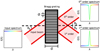 |
Fig. 3 Schematic top-down view of a Bragg grating as an optical component and its effect on a beam. A collimated input beam with a flat spectrum enters the Bragg grating from the left. The grating diffracts the beam into the zeroth and first orders transmission orders. Inside the Bragg grating the refractive index modulation is visualized by the black and white stripes. The Bragg angle θB, grating thickness d, and grating pitch σ are also visualized. Based on Fig. 2 from Haffert et al. (2019b). |
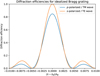 |
Fig. 4 Diffraction efficiencies for transverse electric and transverse magnetic waves transmitted by a Bragg grating with a single-layer antireflection coating, plotted here as a function of deviation from the central Bragg wavelength λB. This grating has a Bragg angle of π/6, a thickness of 500 Bragg wavelengths, and an average index of refraction of 1.4. |
3.2 Multiplexing Bragg gratings
Bragg gratings have another major advantage over regular transmission gratings: multiple Bragg gratings can be created (multiplexed) in the same block of material at the same time. We then refer to them an MBG, a multiplexed Bragg grating. Each of the gratings has its own Bragg wavelength and works largely independently of the others. All the multiplexed gratings in a block of material have to have the same Bragg angle θB, because they all receive the same input beam of light. The ith grating with Bragg wavelength λB,i then sends the light with wavelength λB,i to the 1st diffraction order with that same angle θB (each grating has the setup from Fig. 3, with different σi and λB,i· but the same θB such that Eq. (3) is satisfied). This means that light with wavelengths λB,1, λB,2, λB,3,… ends up having the same output angle θB. Similarly, all light with wavelengths (1 − є)λB,1,(1 − є)λB,2,… for some small number є ends up with the same output angle. This angle will be slightly different from θB due to the gratings’ dispersion (from Eq. (1)). The light that ends up on the detector is then the incoherent sum of the light from each grating separately, that is, we can optically stack the individual spectra transmitted by the respective grating passbands. In practice, this means that the total detector signal is simply the sum of the light seen by each grating. This is visualized in Fig. 5.
Multiplexing Bragg gratings is similar to optically correlating the spectrum of an exoplanet with a reference spectrum. Instead of directly cross-correlating a measured spectrum with a template spectrum, we can multiplex a set of Bragg gratings with Bragg wavelengths around wavelengths of interest. Our detector signal is then the sum of all the individual spectra transmitted by these gratings. Any common features in all spectra will still be present in the total signal, but features only present in a single spectrum will be strongly reduced due to the averaging over individual spectra (Fig. 5). This is what allows us to differentiate between stellar and planetary spectral features.
There is a small difficulty in interpreting the measured detector signal: For a single grating it is possible to plot the measured spectrum as a function of λ − λB, but when multiplexing gratings we have light with multiple wavelengths contributing to a single data point in our spectrum. We therefore cannot plot the spectrum as a function of a single wavelength anymore. Using the relation between wavelength shift and the corresponding Doppler velocity circumvents this issue. The spectrum from the ith grating can be plotted as a function of (λ − λB,i)/λB,i·. This corresponds directly to a Doppler shift δυ:
 (6)
(6)
This Doppler shift is the same for all gratings, which allows us to unambiguously plot the combined spectrum as a function of velocity offset δυ from the Bragg wavelengths. We therefore plot our spectra (see Figs. 8–10) as a function of velocity offset or radial velocity.
A set of multiplexed Bragg gratings incoherently adds light from multiple gratings per spaxel. This increases the S/N per spaxel. In this paper, we estimate the noise based on the variation in the signal at similar wavelengths in other spaxels (see Sect. 4). The expected gain in S/N over a normal spectrograph is approximately given in Haffert et al. (2019b):
 (7)
(7)
where F0 is the average photon flux ratio between the continuum and the selected lines, N the number of gratings, and  the variance of read and dark noise.
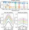 |
Fig. 5 Passbands for example spectra and the process and result of multiplexing several Bragg gratings. The top panel shows two example spectra, one for a planet that contains spectral features we wish to extract and one for a star whose spectral features we want to ignore. The colored bands represent the passbands of five multiplexed Bragg gratings, each chosen to have a Bragg wavelength around a planetary spectral feature. The colors of each band correspond to the line colors in the lower plots, which show the spectra after individual gratings for the star and planet separately, with an offset between the lines for clarity. The individual spectra are plotted as a function of velocity offset that is proportional to the wavelength. The black spectra are the total signals, which have been optically stacked (effectively summed) due to the multiplexed gratings. The stellar spectral features are different for every grating; the optically combined stellar spectrum therefore becomes smoother as more and more gratings are used. On the other hand, the planet has its spectral features of interest aligned due to the choice of Bragg wavelengths, leading to a prominent overall spectral feature. Figure based on Fig. 4 from Haffert et al. (2019b). |
3.3 Bragg grating implementations
Bragg gratings are commonly realized with volume phase holographic (VPH) gratings (Barden et al. 2000) that have the index of refraction modulation permanently inscribed in the base material. Possible base materials for VPHs are polymers (Tomlinson et al. 1976) or photo-thermo-refractive glasses (Glebov 2009) exposed to an ultraviolet interference pattern, or high index glasses inscribed with a femtosecond laser (Richter et al. 2011). For example, a triple VPH is used in Haffert et al. (2020) in a compact Integral Field Unit (IFU). Once manufactured, the index modulation of a VPH is fixed. Multiplexing a large number of gratings in a VPH is difficult, because the incoherent combination of gratings can saturate the base material. Saturation refers to the phenomenon that the inscribed index of refraction modulation δn(x) depends linearly on the applied radiation field U(x) at low intensities, but becomes nonlinear and flattens out at a maximum δnmax for high intensity radiation fields (see Eq. (8) and Fig. 1 in Kaim et al. (2015)). A tunable set of central wavelengths can be accomplished with an acousto-optical tunable filter (AOTF). The AOTF creates the index of refraction modulation by generating high-frequency sound waves in a block of base material (see Bei et al. 2004 for an overview). By coherently superimposing multiple sinusoidal sound waves, it is possible to multiplex a large number of Bragg gratings at the same time without saturating the base material. The sound waves are generated by a piezo element, allowing for a quickly tunable set of multiplexed Bragg gratings controlled by a computer. AOTFs in the optical or near infrared are often made from TeO2 (tellurium dioxide), a uni-axial crystal (Brimrose 2023). We also use the permittivity of TeO2 for the base permittivity matrix of our simulated Bragg gratings. An AOTF can be placed in an optical setup such as the multiplexed Bragg gratings (MBG) shown in Fig. 1 or the Bragg grating in Fig. 3.
3.4 Rigorous coupled wave analysis (RCWA) of multiplexed Bragg gratings
We implement an idealized multiplexed Bragg grating through rigorous coupled wave theory (Moharam & Gaylord 1981). We choose coordinates such that the ẑ-axis is along the surface normal of the grating. The  -axis is chosen such that the input beam is in the
  plane and the ŷ-axis such that the
  axes are a right-handed triplet. The +ẑ and
  are oriented such that the input beam is propagating in the
  and +ẑ directions. Figure 3 shows the
  plane with +ẑ pointing from left to right,
  pointing up, and +ŷ pointing into the page. The Bragg grating then has surfaces of constant refractive index in the ŷ–ẑ plane. Rigorous coupled wave analysis allows us to calculate the effect of the grating on a fully polarized plane wave. A fully polarized plane wave is diffracted by the grating to several reflected and transmitted plane waves, each with their own phase shift and polarization. Our code starts with an input polarized wavefront, which we decompose into a sum of fully polarized plane waves by calculating the angular spectrum of the wavefront. The polarization vector of each plane wave is the sum of two basis vectors (for example,
  and ŷ for a wave propagating in the ẑ-direction). This allows us to write the polarization as a two-component vector x (Bos et al. 2017; McLeod & Wagner 2014). This is different from the coordinate vector
  . When writing x we refer to the polarization vector, and when writing
  we refer to the spatial coordinate. An infinite number of polarization basis vectors e1, e2 for a given wave vector k satisfy the required orthogonality relations e1 • e2 = e1 • k = e2 • k = 0. We use:
![Mathematical equation: $${e_1} = {C_1}\left[ {\matrix{ {{k_z}} \cr 0 \cr { - {k_x}} \cr } } \right],\quad {e_2} = {C_2}\left[ {\matrix{ { - {k_x}{k_y}} \cr {k_x^2 + k_z^2} \cr { - {k_z}{k_y}} \cr } } \right]{\rm{, }}$$](/articles/aa/full_html/2024/06/aa47885-23/aa47885-23-eq21.png) (8)
(8)
with constants C1 and C2 making the length of the two vectors unity. These are unit vectors along the  and ŷ axes if k is parallel to the ẑ axis. The output wave for the 1st transmitted order as calculated by RCWA is a linear transformation of the input wave, so we can calculate a 2 × 2 response matrix Pk per wave vector k for the optic. We calculate the grating output for plane waves with x = [1, 0], [0, 1], which gives us the columns of Pk. Afterward, we obtain the output polarization vector for an arbitrarily polarized wave, represented by a general xk,in, through simple matrix multiplication xk,out = Pk xk,in.
We follow the method of Glytsis & Gaylord (1989) for a rigorous coupled wave theory with multiplexed Bragg gratings. This method allows for an arbitrarily polarized plane wave with arbitrary wave vector to be propagated through a multiplexed set of Bragg gratings and reduces to the Berreman calculus (Berreman 1972) in the case that the index modulation amplitude goes to zero. The methods in Glytsis & Gaylord (1987) allow for multiple layers of materials, which allows us to create antire-flection coatings for the material containing the multiplexed Bragg gratings. In a physical instrument, antireflection coatings over the full bandpass of interest will be necessary to prevent Fabry-Perot fringes (for example the Y, J, H bands for our chosen wavelength range between 1 and 2 micron). We use the idealization that each grating has a separate single-layer coating that is optimized for that grating’s Bragg wavelength, instead of a single (but more complex and multilayer) coating for our entire wavelength range of interest. To include the single-layer coatings on the MBG, we need to make some changes to the original formalism in Glytsis & Gaylord (1987). These are detailed in Appendix A. Since these algorithms assume an infinite extent of each interface, we thereby neglect edge effects. This implementation also neglects the wavelength change caused by the phonon-photon energy exchange in an AOTF (Bei et al. 2004). Because our optical setup does not have any components that are highly sensitive to wavelength after the MBG, we ignore this change in wavelength.
We assume that the multiplexed Bragg gratings can be modeled by a set of independent single gratings. Fu et al. (1997) found that this assumption holds if the Bragg wavelengths of each grating are separated by at least ~3 times the full width at half maximum (FWHM) of the diffraction efficiency curve or passband (see also top panel in Fig. 6). We ensure that this assumption holds in our Bragg wavelength selection. Modeling each grating separately greatly reduces computational and numerical complexity. Although our implementation of the rigorous coupled wave theory can in principle handle multiple gratings, we ran into numerical issues and problems with computation time. Calculating the resulting beam intensities for M gratings, retaining just the zeroth and first order per grating, scales as 2M both in required computation time and storage capacity. If multiple gratings are added (or even a single grating with an input angle very far from normal incidence), some of the eigenmodes in the gratings represent evanescent waves. Evanescent modes have a propagation factor proportional to eΛd for some complex Λ with positive real part. For d >> λ this factor cannot be stored with 64-bit floating point numbers, leading to difficulties with the boundary conditions.
Since the incident and output beams impinge on the Bragg gratings at a nonparaxial angle, applying a tilt correction to the phase does not accurately represent the rotated wavefront. Furthermore, the sampling of the wavefronts is too low to apply the tilt to the wavefront. Attempting to apply the required phase tilt directly would result in serious problems with aliasing. This is solved by separately saving the offset of the beam in k-space, similar to parabasal wavefront propagation (Asoubar et al. 2012). The beam rotation is implemented using the method of Zhang et al. (2013). With this method we interpolate the angular spectrum of the original beam onto the angular spectrum of a set of rotated wave vectors. This also models the beam changing shape due to the rotation, in addition to the tilt offset.
3.5 RCWA code verification
We verified the performance of our RCWA implementation by comparing it to two known results from the literature, and by checking energy conservation in Fig. 6. The top panel of Fig. 6 shows what happens when two multiplexed gratings have similar Bragg wavelengths. The gratings start to influence each other, leading to a lower peak diffraction efficiency for each grating. In the limit where both Bragg wavelengths are the same, we have a single grating with modulation amplitude 2δn (with each grating having a modulation amplitude δn), which also leads to a lower diffraction efficiency. This effect was also found by Fu et al. (1997), who found that a set of coupled gratings can be approximated by a set of independent single gratings as long as all the Bragg wavelengths of all gratings are separated by at least ≳3Δλ. Our result agrees with this. Given a range of wavelengths between λmin and λmax, we can use Eq. (4) to obtain a rough upper limit on the number of multiplexed gratings that we can make in that wavelength range:
 (9)
(9)
For example, using wavelengths between 1 and 2 µm, a Bragg angle of π/6 and grating thickness of a few centimeters, we find an upper limit on the order of ~103 gratings.
The middle panel of Fig. 6 shows our result for energy conservation. A necessary (but not sufficient) requirement for our RCWA code is energy conservation. All the incoming light has to go somewhere; the sum of diffraction efficiencies over all diffraction orders must therefore equal 100% (Moharam & Gaylord 1981). This means 100% of the input energy has gone into a diffraction order. Our RCWA code conserves energy to above a 10−10 relative precision. RCWA requires calculating the eigenvalues, eigenvectors, and inverse of a matrix (see Appendix A). Using more modes than the minimum of two or using more gratings than the minimum of one causes the dimension of those matrices to be larger, leading to bigger numerical errors in their inversion, eigenvalue, or eigenvector determination. Increasing the grating thickness d leads to bigger exponents in the propagation factor computation (these factors are proportional to exp (Λd) for some Λ), leading to larger relative errors in the evaluation of the exponent and the subsequent matrix inversion.
The bottom panel of Fig. 6 compares our DE curve to the analytical prediction by Ciapurin et al. (2005). Our code matches their equation 14 for the DE of the 1st transmitted order to a 10−3 level in the main lobe and 10−2 in the first side-lobes. An exact correspondence is not expected, because Ciapurin et al. (2005) rely on several simplifications to reach their result, but we do not make in our RCWA code. One of these is reflection and transmission at the interfaces, which influences the diffraction efficiency of the main lobe. Ciapurin et al. (2005) neglect the second derivative in the wave equation, leading to differences in the side lobes of the DE curves. They also assume an isotropic material, while our code supports a general permittivity matrix. This allows us to use uni-axial materials such as the TeO2 used in our simulations.
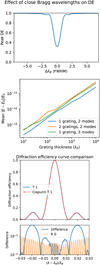 |
Fig. 6 Three simulations for code verification. The first panel shows how the peak diffraction efficiency of two gratings changes as a function of the difference in their central wavelengths. The difference in central wavelength is measured in terms of the FWHM of a diffraction efficiency curve. The second simulation shows energy nonconserva-tion through a slab of material containing one or two Bragg grating(s), with the [0, 1(, 2)] modes used. Any energy nonconservation here stems from numerical errors. The third panel shows the comparison between a diffraction efficiency curve from our RCWA code and an analytically derived diffraction efficiency curve from Ciapurin et al. (2005). The top plot shows the first transmitted order, and the bottom plot shows the difference of the two curves in the top plot and the zeroth reflected order. The differences between our result and Ciapurin et al. (2005) are at or below the level of ~1%. |
4 Data reduction
Each spaxel has a copy of the stellar and planetary spectra, scaled by the value of the telescope PSF (averaged over the different stacked wavelengths cf. Fig. 5). As we want to extract a spectral feature from the exoplanet, we need to remove the appropriate fraction of the stellar spectrum in each spaxel. To recover the stellar and planetary spectra, we let each spaxel count as a separate measurement of a combined spectrum. Our data reduction approach consists of the following steps: we construct an estimate of the stellar spectrum, remove that, and then remove several principal component analysis (PCA) components to determine the planetary spaxel and spectrum. This approach assumes that the stacked spectrum of the star and planet are different enough to avoid light from the planet being removed when subtracting out the stellar spectrum. A flowchart showing the data reduction can be seen in Fig. 7.
Our data reduction is similar to the approach in Landman et al. (2021) (see also Tamuz et al. 2005; Hoeijmakers et al. 2018), because we have a similar set of input data to their approach. The main difference is that they have measurements of the system at different times during a transit. We have a single overall measurement, but every spaxel provides a separate measurement.
We begin by creating a first estimate of the stellar spectrum by taking the brightest spaxels (20 in our case out of a total of 121 fibers) and taking the median of their spectra. We do a first pass on reducing the data by removing a scaled version of this spectrum from every spaxel. The scale can be chosen as the average intensity in each spaxel; however, we can improve this slightly by taking the low-frequency information in each spaxel’s spectrum into account. For each spaxel we divide out the first estimate of the stellar spectrum, and then smooth the result with a Gaussian kernel to reduce any narrow spectral features but preserve the continuum information. The width of this kernel is 40 pixels, corresponding to around half of the main diffraction-efficiency lobe. The model stellar spectrum for that spaxel is then the product of this smoothed ratio and the first estimate of the stellar spectrum. Afterwards we remove a variable number of PCA components (typically up to three for the results presented here) for any leftover residuals brighter than the exoplanet. The number of PCA modes to remove depends on the contrast.
We make an estimate of the noise level (which may be due to photon noise or PCA residuals) for each velocity offset using spaxels not containing the planet. We divide the reduced data cube with residuals by these noise estimates to obtain an S/N estimate for the spectrum in the planet spaxel. This approach treats any residuals as noise, so the PCA residuals can be considered a type of systematic noise. The overall S/N is then found by taking the maximum S/N found in the planet spectrum between velocity offsets of −10 and 40 km s−1. This is an interval around the main absorption feature in the simulations and excludes any spuriously high S/N near the edges of the main diffraction-efficiency lobe. The S/N curve as a function of velocity offset will generally have a slightly different shape than the raw residuals, because the noise estimation is done separately for each velocity offset.
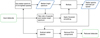 |
Fig. 7 Flowchart describing the approach for the data reduction. See the text more details. |
5 Results
5.1 Single simulation
Figure 8 shows the resulting intensities for each of the 20 gratings. The Bragg wavelengths are chosen based on the strength of a CH4 absorption feature, but in the total petitRADTRANS spectrum not all of these absorption features have the same line depth. Most of these features are also quite shallow compared to the continuum (ΔI/I ~ 10−2−10−1 for most gratings. This results in an overall absorption feature of around 7% compared to a flat spectrum. The (in this case small) depths of the CH4 absorption features depend on the planetary properties, which we do not include in our Bragg wavelength selection.
The stellar spectrum in Fig. 8 shows several spectral features present in different gratings. However, all these features are at different velocity offsets, so they average out in the total intensity curve to a 1% variation compared to a flat spectrum. In the planetary spectrum all absorption features are at the same velocity offset, so they combine into an overall absorption feature. This is analogous to the schematic shown in Fig. 5.
The result after post-processing a data cube with stellar light and a planet at 10−6 contrast is shown in Fig. 9. It shows the planet being reconstructed at the correct spatial position with its main spectral feature. The S/N estimate for this reconstruction is 30. The planet is most clearly visible when comparing between spaxels at the appropriate velocity offset, however, the planet’s spectrum has some extra features compared to the intensities shown in Fig. 8. A similar result (albeit with lower S/N) is found when using a flat spectrum for the planet. This seems a general feature in the data reduction, where the planet spaxel is very clearly identified, but the spectrum of the planet spaxel has extra features or deviates significantly from the input planet spectrum.
The extra features in the spectrum of Fig. 9 can be explained by comparing it to Figs. 10 and 8. The right panel of Fig. 10com-pares the residuals of a cube with the petitRADTRANS spectrum and a flat spectrum for the planet. The extra features in the spectrum of Fig. 9 are also present in the residuals for a planet with a flat input spectrum, suggesting they are not caused by light from the planet, but rather light from the star. In fact, the 1% variation in the bottom right panel of Fig. 8 matches these features as well. We therefore attribute the extra residuals to the small variations in the stacked stellar spectrum. These variations are from individual stellar lines in the MBG’s passbands. Even though the planet spaxel can often clearly be identified, the stellar spectrum can have an impact on the reconstructed spectrum.
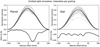 |
Fig. 8 Simulated detector intensities for the planet and star for a single fiber containing the Airy core of the respective source. In the top panels, the gray lines show the results for each of the 20 individual Bragg gratings, with the black line showing the total response of the multiplexed Bragg grating, which is the sum of all gratings. The large, Gaussian-shaped intensity profile is due to the wavelength-dependent transmission of the grating. In the bottom panels we show the ratio between these total responses and the response to a flat input spectrum as a measure of the average spectrum seen by the instrument. |
5.2 Varying the number of multiplexed gratings
Multiplexing multiple gratings has an effect on the final, reduced image even without the addition of photon noise. This is shown in Fig. 11, where it is shown that the deepest contrast found with an S/N > 5 improves with lower grating numbers. This is due to two main factors: The first factor is that every new grating adds an extra variation to the stellar spectrum per spaxel. This is because of the stacking of several PSFs of different wavelengths. Within a passband of ~ ± 100 km s−1, we have a relative change of ~7 × 10⁻⁴ in the size of 1 λ/D. The different Bragg wavelengths for each grating correspond to a change in λ/D of a little over 3% in our simulations. This mainly leads to small variations in the continuum for each spaxel, resulting in different spectral estimates for each spaxel. This will depend on how far away the spaxel is from the center of the PSF. Removing a larger number of PCA components can partially compensate this effect, but it will always leave some residuals. Adding more gratings will leave more residuals at a fixed number of removed PCA components and decrease performance at deep contrasts.
The second factor is our chosen set of passbands. This leads to the previously discussed result that not every grating we use in our simulations has an equally prominent absorption feature. If light is added from a relatively flat passband by a grating, this will reduce the relative strength of the overall absorption feature compared to the PCA residuals. This lowers the overall S/N, which is especially visible in the ‘8 gratings’ line. It has a lower overall S/N and has similar performance to 12 gratings at deep contrasts. The PCA residuals are the noise source in our S/N for this figure, and an improved line selection method will have better performance than the results from our simple line selection method.
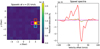 |
Fig. 9 Example reduced data cube with a 10−6 planet with its own emission spectrum located at the (4, 0) fiber. The image is scaled to the maximum intensity in the cube before data reduction. The left panel shows the absolute signal per fiber at a velocity offset of 21 km s−1. The right shows the spectra of several spaxels around the simulated planet signal, with the corresponding spaxels colored in the left panel. This data cube was reduced without the addition of detector noise but with the addition of photon noise and a closed-loop AO simulation. |
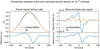 |
Fig. 10 Comparison between results from the petitRADTRANS simulated emission spectrum and a flat emission spectrum for the planet without the addition of any noise. The left panel shows the spectra of the planet spaxel without the addition of any stellar light, with the difference of the two curves plotted below. The right panel shows the residuals of analyzed data cubes with stellar and planetary light for the two planetary spectra. The planet contrast in these data cubes is set to 10−6 and at a separation of ~3λ/D. The bottom panel again shows the difference between the curves. |
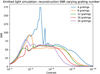 |
Fig. 11 Peak signal to noise for the reconstructed exoplanet absorption feature as a function of contrast, varying the number of multiplexed gratings. The number of removed PCA components is in the range 0– 3 and is chosen per contrast to maximize the S/N. These cubes were reduced without the addition of detector or photon noise, but included a closed-loop AO system. |
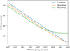 |
Fig. 12 Limiting contrast (deepest contrast with a S /N > 5 planet reconstruction) as a function of photon count for various numbers of grating. The planet is at a distance of 4λ/D from the star. The reference intensity Iref is the maximum intensity found in a single pixel in the data cube for a single grating before the addition of photon noise. Each plotted point is the result of ten instances of photon noise being averaged. |
5.3 Contrast limits
We define the limiting contrast as the deepest contrast where the planet can still be reconstructed with a signal-to-noise ratio >5. Figure 12 shows this limiting contrast as we change the amount of photon noise added to our data. The slight noisiness of each plotted line is because of specific instances of photon noise sometimes allowing a slightly fainter planet to be detected, and sometimes not.
For limiting contrasts down to ~ 10−7 photon noise is the limiting factor in the reconstruction, which produces the expected  relation between limiting contrast and photon number. From Fig. 11 it can be seen that no matter how many gratings we include in our data reduction, the S/N without photon noise is well above 5 in this range, so this does not influence our limiting contrast. Every extra grating puts more photons on the detector, pushing the limiting contrast down by an extra factor
  . Deviations from this factor are from the different continuum levels in each grating passband. If, for example, the continuum in the sixth grating lies slightly higher than the average of the first five gratings, we will obtain slightly more photons than expected, that is, our limiting contrast lowers by a bit more than the expected (6/5)−1/2.
As the number of photons increases, the dominant source of residuals will switch from photon noise to the PCA residuals. As discussed in Sect. 5.2, adding more gratings with our current data reduction leads to decreased performance at deep contrasts. This causes the limiting contrast curves to level out in the opposite order compared to when the data reduction is limited by photon noise. There is a crossover region between these two limiting cases, where using a higher number of gratings produces a comparable result to using a lower number of gratings. The location of this crossover region in general depends on the number of gratings used. Our simulations suggest that for contrasts below 10−7 our current approach for the data reduction is not sufficient when multiplexing >20 gratings, but this result will change based on the specific Bragg wavelengths and spectra of the star and planet.
Figure 13 shows the limiting contrast for different separations between star and planet. It follows the same qualitative structure as Fig. 12, with photon noise-limited contrasts at lower photon counts that level off as the photon noise levels drop below the PCA residuals. As usual the contrast determines the ratio of peak intensities for the star and planet data cubes, so the limiting contrast scales with the relative intensity of the stellar PSF at a given separation. As our simulations are run without any coronagraphic elements, these can be used to deepen the limiting contrast further (see for example SCAR from Por & Haffert 2020, given our use of a single-mode fiber array).
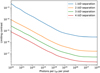 |
Fig. 13 Limiting contrast (deepest contrast with a S /N > 5 planet reconstruction) as a function of separation between the star and planet. The reference intensity Iref is the maximum intensity found in a single pixel in the data cube for a single grating before the addition of photon noise. Each plotted point is the result of ten instances of photon noise being averaged. |
6 Discussion
The simulations described in the previous sections make some idealized assumptions that cannot be made in an actual instrument; for instance, the simulations do not consider parameters such as beam diameters, the size of the gratings, or the layout of the fiber array. When converting our simulated optical setup to a physical instrument, however, these are critical considerations. We therefore discuss issues that may arise when designing an instrument with multiplexed Bragg gratings.
6.1 Multiplexed Bragg gratings in an instrument
A system similar to the simulation layout as in Fig. 1 should be possible to implement as an instrument in an existing telescope without any major difficulties. The micro-lens array can be implemented at any available focus in the telescope, with a fiber bundle possibly leading to a Nasmyth platform where the collimator, MBGs, and detector can be placed. The use of a fiber bundle gives flexibility in the positioning of the instrument. As the MBGs functions as a transmission grating, the layout of our approach is similar to an instrument with a transmission grating (see Haffert et al. 2019b).
An important parameter to consider when designing an instrument using an MBG is the required beam size Dbeam on the grating. This depends on the requirements of the instrument, such as the desired spectral (or equivalently velocity) resolution. The effects of varying the velocity resolution and Bragg angle are plotted in Fig. 14. The required beam size on the grating scales directly with the desired resolving power R ~ Dbeam as for any diffraction grating, but the Bragg angle adds an additional degree of freedom. In addition to controlling the projected beam size (the incoming beam enters at the Bragg angle), the Bragg angle also changes the spectral selectivity of the grating following Eq. (4). In particular, Bragg angles ≲π/10 can increase the required beam size by an order of magnitude compared to Bragg angles around π/4.
6.2 Fiber reformatting
We can reformat the fiber array between its input and output and/or the optics behind the fiber array to optimally use the multiplexed Bragg gratings. Using the same rectangular fiber array layout for the input and the output is not a viable option; if we collimate each fiber separately we end up with a set of submillimeter-sized beams, whose footprints on the grating are too small to achieve the spectral resolution we require. If we collimate all fibers with a single lens we end up with a set of overlapping beams, each propagating at a slightly different angle. This is a problem for the difference in angle in the  plane, because most beams will not enter the grating at the Bragg angle. This leads to different (and possibly very poor) DE for those beams. We must therefore choose a different layout for the fiber array output. We consider three options:
We replace the lenses L2 and L3 with lens arrays and increase the spacing between the fibers to create a set of larger colli-mated beams. Each beam will be completely separated from the others and have the beam diameter required to reach our desired spectral resolution of ~105;
We format the fibers to lie in a single line in the ŷ direction, creating a set of collimated beams with a slightly different propagation directions in the ŷ – ẑ plane (cf. Haffert et al. 2019b);
We swap the MBG and the lens L3, letting a set of converging beams pass through the Bragg gratings.
In our simulations, we use the first arrangement, because the Bragg grating responds to every fiber in the same way in this case, which significantly reduces the computational complexity. This also means that the final detector images of each fiber are well separated (by the diameter of each beam). For any real instrument, however, this arrangement is not feasible due to size limitations on the grating size. With our chosen fiber array we would need a grating of size 11Dbeam × 11Dbeam. In our simulations we have Dbeam = 22 cm (see Table 1). The grating is then around 2 × 2 meters, which is unworkable.
The arrangement of all fibers in a line (similar to a pseu-doslit) is not affected by this problem, because in that case all beams overlap at the grating. The grating size is then only approximately the size of a single beam, regardless of the number of fibers. There are now two angles to consider: each beam enters at the Bragg angle in the  plane, but at different angles in the ŷ–ẑ plane. The grating response will be slightly different for each fiber because of this. The effect of changing the angle in the ŷ– ẑ plane (equivalent to changing ky in the incoming wave vector k) is shown in Fig. 15. A nonzero ky for a beam will change the output polarization to lowest order, but will also see decreased diffraction efficiency as its angle increases. If polarization is of interest, either the desired polarization state must be selected before reaching the grating, or the entire instrument must be modeled and/or calibrated carefully to remove the systemically induced polarization. If polarization is not of interest, varying ky has an effect on diffraction efficiency. For angles <10 degrees this effect is only around 1%, and so does not require any significant correction apart from calibration.
Swapping the final lens L3 and the grating runs into trouble, again because of the angular selectivity of the Bragg gratings in the  plane. For a moment we consider a converging beam as consisting of a set of rays. Generally a ray in this set will be at an angle to the optical axis due to the converging nature of the beam. The largest such angle in the converging beam is 1/(2F) for a focal ratio F. A volume Bragg grating requires angles to be in the range [θB–δθ, θB + δθ] to be within the main lobe of the diffraction-efficiency curve, where
  (Ciapurin et al. 2005). The focal ratio of the beam must therefore be larger than
  to not have the beam distorted by the grating. The diffraction efficiency curve Eq. (2) acts as a virtual slit, suppressing light coming in at angles outside the above range. A collimated circular beam also has an angular spread ~λ/Dbeam in its constituent plane waves, giving a requirement
  . For d ~ 1 cm and σ ~ 1 µm, this gives F ≳ 103 and Dbeam > 104λ. This means that a converging beam is not feasible for the above parameters, and a collimated beam with a diameter of at least ~1 cm is needed.
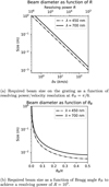 |
Fig. 14 Effect of varying the Bragg angle or desired resolving power R on the required beam diameter per fiber. Beams with smaller diameters than given here will limit spectral resolution, due to the PSFs per wavelength growing larger without a corresponding increase in separation. The top plot shows the linear relationship between R and beam diameter (and illuminated lines), which is standard for transmission gratings. The bottom plot shows the effect of varying the Bragg angle. |
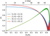 |
Fig. 15 Polarization change in the first order transmitted plane wave for an incoming plane wave at the Bragg wavelength and incoming wavevector k, with kX tuned to the Bragg angle, but with a varying ky. The lines for [0, 1] → [1,0] and [1,0] → [0,1] overlap. The lower transmission of the [0,1] → [0,1] mode can also be seen in Fig. 4, and the thicker lines at higher |ky| are unresolved Fabry-Perot fringes. |
6.3 Compressed sensing
Using MBGs for compressed sensing provides several advantages, some general to compressed sensing and some specific to MBGs. As shown in Eq. (7) and Fig. 12 we obtain a reduction in relative detector and photon noise proportional to  , compared to approaches using only a single passband or recording each passband separately. This is also accompanied by a reduction in detector pixels used for spectral resolution of Ngratings. Each new passband is stacked on top of previous ones, rather than requiring a new spot on the detector. By multiplexing the gratings in one block of material we also enable a compact instrument, as all gratings are present in one optical component. MBGs also give us significant freedom in the passbands we select, with extremely narrow passbands (Δλ/λ ~ 10−3 in our simulations) able to be picked with (if desired) a wide spread in central wavelengths. Commercially available AOTFs, for example, allow central wavelengths to be picked over a range of Δλ/λ ~ 0.5 (Brimrose 2023).
Although the MBGs allow for stacking of a mostly arbitrary set of passbands, there is a downside to this compressed sensing approach as well. With a full spectrum it is possible to look for arbitrary spectral features after having taken a measurement, so one can cross-correlate with several template spectra to try to find multiple molecules. This is not possible with our approach. As all passbands are stacked on top of each other, parallel measurements of (for instance) multiple molecules are not possible. Every new molecule to be measured requires a new measurement with a different set of MBG settings. This is partially compensated by the shorter time per measurement, which is the result of the lower detector noise per Eq. (7), as well as the reduced effect of photon noise by optically stacking each passband. If the MBG is implemented using an AOTF, the different Bragg gratings can be altered by changing the acoustic waves. As the speed of sound in crystal is on the order of several km s−1, a new acoustic signal can propagate through the entire AOTF in sub-millisecond timescales. This means it is possible to quickly and arbitrarily switch a set of passbands during an observation, if measurements for multiple species are desired.
7 Conclusion
We described our implementation of a rigorous coupled wave code to simulate multiplexed Bragg gratings, based on the formalism of Glytsis & Gaylord (1987, 1989) (Sect. 3.4 and Appendix A). We verified this code to have energy conservation and agree with literature results (Fig. 6). With this code we have presented an end-to-end simulation of an optical system containing multiplexed Bragg gratings, containing up to 20 separate Bragg gratings (Fig. 1). We included simulated source spectra based on the HR8799 system for a star and exoplanet system, a simplified closed-loop adaptive optics system, and modeled the multiplexed Bragg grating using our own implementation of rigorous coupled wave theory. Our simulations show that it is possible to recover a stacked CH4 absorption feature with its Doppler shift from an exoplanet down to contrasts around 10−6–10−7 (the exact limiting contrast depends on telescope diameter and AO residuals) when not limited by shot noise. The relation between the deepest contrast we were able to reconstruct for different numbers of multiplexed gratings can be seen in Figs. 11 and 12, with 13 showing the lower contrast limit for various separations. Specifically we confirmed that deeper contrasts can be reached with multiple multiplexed gratings when limited by photon noise. We also found that at deep contrasts and high photon counts our data reduction approach based on principal-component analysis limits the deepest achievable contrast. Using a higher number of stacked gratings adds more spectral variations per spaxel, which PCA has difficulty removing.
The optical setup as presented here is not the only way to include a multiplexed Bragg grating in an instrument. We have already discussed some options for rearranging the fibers in the fiber bundle, but not including a fiber bundle at all is also a possibility (this is already done when using an AOTF as a filter, see for example Dekemper et al. 2016). When using multiplexed Bragg gratings as an IFU, spectral and spatial information are mixed, but this could be addressed by taking a set of measurements with different spatial offsets of the target per measurement. The spatial and spectral information can then be disentangled. Multiplexing a large set of gratings is possible in principle in an AOTF (see Haffert et al. 2019b), but testing an AOTF’s ability as a spectrometer with multiple stacked gratings is important to test. The data reduction as presented in this paper can also likely be improved on. We have used a general PCA to remove residuals, but this general method does not use any of the extra information we have (such as the set of Bragg wavelengths or the position of each spaxel in the focal plane). A different approach that includes this information will likely give better results, especially at deep contrasts.
The code to run the simulations in this paper is written in Python 3.7, and we have made extensive use of the packages numpy and matplotlib (Harris et al. 2020; Hunter 2007). This research made use of HCIPy, an open-source object-oriented framework written in Python for performing end-to-end simulations of high-contrast imaging instruments (Por et al. 2018).
Acknowledgements
We acknowledge funding from the NWO-TTW SYNOPTICS program, and co-funding from Airbus D&S NL. The authors would also like to thank Rico Landman, David Doelman, and Frans Snik for helpful discussions. We also thank the anonymous referee for their feedback and many helpful comments.
Appendix A Rigorous coupled wave theory reformulation
To construct the simulation framework we combined the results from Glytsis & Gaylord (1987) and Glytsis & Gaylord (1989) to support a stack of materials, where a single layer of material may contain multiple gratings. This is necessary to be able to add antireflection coatings to the AOTF model, which removes Fabry-Perot fringes in the final diffraction efficiency curve. We also reformulated their results to have the propagation direction be the +z axis rather than the −y axis, which is more in line with the standards used in optics and software environments such as hcipy. For more information on the steps mentioned here, we refer to the above-mentioned papers and their appendices.
We divide space up into three regions: region 1 has an isotropic material where the incident beam and reflected orders exist, region 2 contains the grating and any other possible layers of material in the stack, and region 3 has an isotropic material where the transmitted orders exist. In region 2 we have L layers with possibly different permittivity matrices and gratings, which are indexed with l and have a uniform thickness sl. All the interfaces between layers are assumed to be infinite and parallel to each other. Grating modes under consideration are the same for each grating and are integers m1 ≤ ml ≤ m2 for some fixed m1, m2 (the simplest case is typically m1 = 0, m2 = 1). For N total gratings, the total number of modes is then M = (1 + m2 − m1)N. The grating modes for the n-th grating are indicated with mn. We will also use the shorthand I for a specific mode combination m1 m2… mN, so  .
.
Due to the gratings the permittivity matrix in the l-th region has the form
 (A.1)
(A.1)
where the hn are Fourier components, the matrices  give the amplitude of each grating for each Fourier component of the grating, and el0 is the base permittivity matrix of the material. The vectors Kn are the grating vectors and determine the kx, ky offsets for each grating order. We have wavevector components k(x,y)l = k1(x,y) − Σn mnKn(x,y) per grating order.
We assume the original source is a fully polarized plane wave in the first region, with polarization vector u and wave vector k1 satisfying |k1| = k0n1 and k1 • u = 0, where n1 is the refractive index in the first region and k0 = 2π/λ the vacuum wavenum-ber. The gratings create a set of 2M new plane waves for the M reflected and M transmitted orders. The reflected orders have wavevectors [kxI, kyI, k1zI]⊤ and the transmitted orders have wavevectors [kxI, kyI, k3zI]⊤. The z-components k1zI and k3zI ensure the final wavevectors satisfy  .
.
The electric field amplitudes of each reflected (transmitted) order are given by RI (TI) and satisfy RI • k1I = TI • k3I = 0. In region 2 the electric field of each layer is written as
![Mathematical equation: $${E_{2l}}(x,y,z) = \sum\limits_{n,{m_n}} {{S_{II}}} (z)\exp \left[ { - i\left( {{k_{xI}}x + {k_{yI}}y - {k_{2zI}}z} \right)} \right],$$](/articles/aa/full_html/2024/06/aa47885-23/aa47885-23-eq37.png) (A.2)
(A.2)
and the magnetic field is similarly written as
![Mathematical equation: $${H_{2l}}(x,y,z) = {\left[ {{{{_0}} \over {{\mu _0}}}} \right]^{{1 \over 2}}}\sum\limits_{n,{m_n}} {{U_{II}}} (z)\exp \left[ { - i\left( {{k_{xI}}x + {k_{yI}}y - {k_{2zI}}z} \right)} \right]{\rm{, }}$$](/articles/aa/full_html/2024/06/aa47885-23/aa47885-23-eq38.png) (A.3)
(A.3)
where k2zI = − Σn mnKnz. We take z = 0 as the start for each layer, so E2l and H2l are defined in the region 0 ≤ z ≤ sl.
Maxwell’s equations for E2l and H2l lead to a linear differential equation Vl(z)′ = iAlVl(z), where Vl(z) = [SlxI, SlyI, UlxI, UlyI]⊤ is a column vector with 4M components (4 per mode, because Maxwell’s equations do not produce differential equations for the SlzI and UlzI), and Al is a 4M × 4M matrix:
 (A.4)
(A.4)
where the aij are M × M sub-matrices:

The  are M × M matrices with k(x,y,z)I along the diagonal for each mode, and the
  are the spatial components of the total permittivity matrices for the layer, taking into account the mode coupling caused by the grating through off-diagonal elements caused by nonzero
  .
.
The solution for each region l is then Vl(z) =  , where Wl = [Wl1, Wl2, Wl3, Wl4]⊤ and
  are matrices with the eigenvectors and the eigenvalues of iAl. The sub-matrices Wl1 to Wl4 all have size M × 4M. The electric and magnetic field components gain an additional phase contribution from the complex exponential in Eqs. A.2 & A.3 and at every interface we have continuity of the tangential components of the electric and magnetic field, leading to the following boundary conditions

where δ is the Kronecker delta. The S and U components at the end of the stack can be rewritten using the boundary conditions between regions, which give Vl(0) = Vl–1(sl–1). Together with the solution  this gives
  , where
![Mathematical equation: $$\eqalign{ & B = W_L^{ - 1}\left[ {{W_{L - 1}}\exp \left( {{{\tilde \lambda }_{L - 1}}{s_{L - 1}}} \right)W_{L - 1}^{ - 1}} \right] \cr & \quad \left[ {{W_{L - 2}}\exp \left( {{{\tilde \lambda }_{L - 2}}{s_{L - 2}}} \right)W_{L - 2}^{ - 1}} \right] \ldots \left[ {{W_1}\exp \left( {{{\tilde \lambda }_1}{s_1}} \right)} \right]. \cr} $$](/articles/aa/full_html/2024/06/aa47885-23/aa47885-23-eq50.png) (A.5)
(A.5)
The boundary conditions and orthogonality requirements for RI, TI give a unique solution for all the unknowns  . The solution satisfies the linear system of equations
 (A.6)
(A.6)
where P11,P12, P13, P14 are M × 4M sub-matrices and p1, p2 vectors of length M. The zeros above are zero vectors of length M. Each component of p1 , p2 corresponds to a unique mode, and has a corresponding set m1m2… mN. The above sub-matrices and vectors have the values
![Mathematical equation: $$\eqalign{ & {P_{11}} = \left( {{{\tilde k}_y}\tilde k_{1z}^{ - 1}{{\tilde k}_x}} \right){W_{11}} + \left( {{{\tilde k}_y}\tilde k_{1z}^{ - 1}{{\tilde k}_y} + {{\tilde k}_{1z}}} \right){W_{12}} + {k_0}{W_{13}}, \cr & {P_{12}} = \left( {{{\tilde k}_x}\tilde k_{1z}^{ - 1}{{\tilde k}_x} + {{\tilde k}_{1z}}} \right){W_{11}} + \left( {{{\tilde k}_x}\tilde k_{1z}^{ - 1}{{\tilde k}_y}} \right){W_{12}} - {k_0}{W_{14}}, \cr & {P_{13}} = \left[ {\left( {{{\tilde k}_y}\tilde k_{3z}^{ - 1}{{\tilde k}_x}} \right){W_{L1}} + \left( {{{\tilde k}_y}\tilde k_{3z}^{ - 1}{{\tilde k}_y} + {{\tilde k}_{3z}}} \right){W_{L2}} + {k_0}{W_{L3}}} \right]\exp \left( {{\lambda _L}{s_L}} \right), \cr & {P_{14}} = \left[ {\left( {{{\tilde k}_x}\tilde k_{3z}^{ - 1}{{\tilde k}_x} + {{\tilde k}_{3z}}} \right){W_{L1}} + \left( {{{\tilde k}_x}\tilde k_{3z}^{ - 1}{{\tilde k}_y}} \right){W_{L2}} - {k_0}{W_{L4}}} \right]\exp \left( {{\lambda _L}{s_L}} \right), \cr & {\left( {{p_1}} \right)_I} = {\delta _{{m_1}{m_2} \ldots {m_N},00 \ldots 0}}\left[ {{u_x}{k_{yI}}k_{1zI}^{ - 1}{k_{xI}} + {u_y}\left( {k_{yI}^2k_{1zI}^{ - 1} + {k_{1zI}} - {k_{1z}}} \right) + {u_z}{k_{1y}}} \right], \cr & {\left( {{p_2}} \right)_I} = {\delta _{{m_1}{m_2} \ldots {m_N},00 \ldots 0}}\left[ {{u_x}\left( {k_{xI}^2k_{1zI}^{ - 1} + {k_{1zI}} - {k_{1z}}} \right) + {u_{yy}}{k_{xI}}{k_{1zI}}{k_{yI}} + {u_z}{k_{1x}}} \right], \cr} $$](/articles/aa/full_html/2024/06/aa47885-23/aa47885-23-eq53.png) (A.7)
(A.7)
References
- Allard, F. 2014, in Exploring the Formation and Evolution of Planetary Systems, 299, eds. M. Booth, B. C. Matthews, & J. R. Graham, 271 [NASA ADS] [Google Scholar]
- Asoubar, D., Zhang, S., Wyrowski, F., & Kuhn, M. 2012, Opt. Express, 20, 23502 [CrossRef] [Google Scholar]
- Bacon, R., Accardo, M., Adjali, L., et al. 2010, SPIE Conf. Ser., 7735, 773508 [Google Scholar]
- Barden, S. C., Arns, J. A., Colburn, W. S., & Williams, J. B. 2000, PASP, 112, 809 [NASA ADS] [CrossRef] [Google Scholar]
- Bei, L., Dennis, G. I., Miller, H. M., Spaine, T. W., & Carnahan, J. W. 2004, Progr. Quant. Electron., 28, 67 [NASA ADS] [CrossRef] [Google Scholar]
- Berreman, D. W. 1972, J. Opt. Soc. Am., 62, 502 [NASA ADS] [CrossRef] [Google Scholar]
- Beuzit, J. L., Vigan, A., Mouillet, D., et al. 2019, A&A, 631, A155 [NASA ADS] [CrossRef] [EDP Sciences] [Google Scholar]
- Bos, S. P., Haffert, S. Y., & Keller, C. U. 2017, SPIE Conf. Ser., 10407, 1040709 [NASA ADS] [Google Scholar]
- Brimrose 2023, Acousto-optical tunable filters datasheet, https://www.brimrose.com/free-space-ao/acousto-optic-tunable-filters [Google Scholar]
- Cepa, J., Aguiar-Gonzalez, M., Bland-Hawthorn, J., et al. 2003, in Instrument Design and Performance for Optical/Infrared Ground-based Telescopes, 4841, eds. M. Iye, & A. F. M. Moorwood, International Society for Optics and Photonics (SPIE), 1739 [NASA ADS] [CrossRef] [Google Scholar]
- Ciapurin, I. V., Glebov, L. B., & Smirnov, V. I. 2005, in Practical Holography XIX: Materials and Applications, 5742, eds. T. H. Jeong, & H. I. Bjelkhagen, International Society for Optics and Photonics (SPIE), 183 [NASA ADS] [CrossRef] [Google Scholar]
- Dekemper, E., Vanhamel, J., Van Opstal, B., & Fussen, D. 2016, Atmos. Meas. Tech., 9, 6025 [NASA ADS] [CrossRef] [Google Scholar]
- Eisenhauer, F., Abuter, R., Bickert, K., et al. 2003, in Instrument Design and Performance for Optical/Infrared Ground-based Telescopes, 4841, SPIE, 1548 [CrossRef] [Google Scholar]
- Fu, X., Fay, M., & Xu, J. M. 1997, Opt. Lett., 22, 1627 [NASA ADS] [CrossRef] [Google Scholar]
- Glebov, L. B. 2009, J. Hologr. Speckle, 5, 77 [CrossRef] [Google Scholar]
- Glytsis, E. N., & Gaylord, T. K. 1987, J. Opt. Soc. Am. A, 4, 2061 [CrossRef] [Google Scholar]
- Glytsis, E. N., & Gaylord, T. K. 1989, Appl. Opt., 28, 2401 [NASA ADS] [CrossRef] [Google Scholar]
- Gordon, I., Rothman, L., Hill, C., et al. 2017, JQSRT, 203, 3 [NASA ADS] [CrossRef] [Google Scholar]
- Gray, R. O., & Kaye, A. B. 1999, AJ, 118, 2993 [NASA ADS] [CrossRef] [Google Scholar]
- Haffert, S. Y., Bohn, A. J., de Boer, J., et al. 2019a, Nat. Astron., 3, 749 [Google Scholar]
- Haffert, S. Y., Por, E. H., & Keller, C. U. 2019b, Opt. Express, 27, 33925 [NASA ADS] [CrossRef] [Google Scholar]
- Haffert, S. Y., Harris, R. J., Zanutta, A., et al. 2020, J. Astron. Telescopes Instrum. Syst., 6, 045007 [NASA ADS] [Google Scholar]
- Harris, C. R., Millman, K. J., van der Walt, S. J., et al. 2020, Nature, 585, 357 [NASA ADS] [CrossRef] [Google Scholar]
- Hoeijmakers, H. J., Schwarz, H., Snellen, I. A. G., et al. 2018, A&A, 617, A144 [NASA ADS] [CrossRef] [EDP Sciences] [Google Scholar]
- Hunter, J. D. 2007, Comput. Sci. Eng., 9, 90 [NASA ADS] [CrossRef] [Google Scholar]
- Kaim, S., Mokhov, S., Divliansky, I., et al. 2015, J. Opt. Soc. Am. A, 32, 22 [NASA ADS] [CrossRef] [Google Scholar]
- Kogelnik, H. 1969, Bell Syst. Tech. J., 48, 2909 [NASA ADS] [CrossRef] [Google Scholar]
- Landman, R., Sánchez-López, A., Mollière, P., et al. 2021, A&A, 656, A119 [NASA ADS] [CrossRef] [EDP Sciences] [Google Scholar]
- Macintosh, B., Graham, J. R., Ingraham, P., et al. 2014, PNAS, 111, 12661 [NASA ADS] [CrossRef] [Google Scholar]
- Marois, C., Macintosh, B., Barman, T., et al. 2008, Science, 322, 1348 [Google Scholar]
- McLeod, R. R., & Wagner, K. H. 2014, Adv. Opt. Photon., 6, 368 [NASA ADS] [CrossRef] [Google Scholar]
- Moharam, M. G., & Gaylord, T. K. 1981, J. Opt. Soc. Am., 71, 811 [NASA ADS] [CrossRef] [Google Scholar]
- Mollière, P., Wardenier, J. P., van Boekel, R., et al. 2019, A&A, 627, A67 [Google Scholar]
- Por, E. H., & Haffert, S. Y. 2020, A&A, 635, A55 [NASA ADS] [CrossRef] [EDP Sciences] [Google Scholar]
- Por, E. H., Haffert, S. Y., Radhakrishnan, V. M., et al. 2018, Proc. SPIE, 10703, 1070342 [Google Scholar]
- Richter, D., Voigtländer, C., Becker, R., et al. 2011, in 2011 Conference on Lasers and Electro-Optics Europe and 12th European Quantum Electronics Conference (CLEO EUROPE/EQEC), 1 [Google Scholar]
- Snellen, I. A. G., de Kok, R. J., de Mooij, E. J. W., & Albrecht, S. 2010, Nature, 465, 1049 [Google Scholar]
- Snellen, I., de Kok, R., Birkby, J. L., et al. 2015, A&A, 576, A59 [NASA ADS] [CrossRef] [EDP Sciences] [Google Scholar]
- Tamuz, O., Mazeh, T., & Zucker, S. 2005, MNRAS, 356, 1466 [Google Scholar]
- Tomlinson, W., Chandross, E., Weber, H., & Aumiller, G. 1976, Appl. Opt., 15, 534 [NASA ADS] [CrossRef] [Google Scholar]
- Virtanen, P., Gommers, R., Oliphant, T. E., et al. 2020, Nat. Meth., 17, 261 [Google Scholar]
- Wang, J. J., Ruffio, J.-B., Morris, E., et al. 2021, AJ, 162, 148 [NASA ADS] [CrossRef] [Google Scholar]
- Zhang, S., Zhong, H., Asoubar, D., Wyrowski, F., & Kuhn, M. 2013, in Optical Systems Design 2012, 8550, eds. L. Mazuray, R. Wartmann, A. P. Wood, M. C. de la Fuente, Tissot, J. M. Raynor, D. G. Smith, F. Wyrowski, A. Erdmann, T. E. Kidger, S. David, & P. Benítez, International Society for Optics and Photonics (SPIE), 85503I [CrossRef] [Google Scholar]
All Tables
Simulation parameters for the telescope, micro-lens array, fiber bundle, and the multiplexed Bragg gratings.
Parameters used in the petitRADTRANS calculation of the planetary emission spectrum and selection of the BT-Settl stellar spectrum.
All Figures
|
Fig. 1 Layout of the optical system in our simulations. The light starts in the upper left corner, being propagated to a fiber array. The output of the fiber array is passed through the set of multiplexed Bragg gratings and focused onto the detector. See the text in Sect. 2.1 for more details. |
| In the text | |
|
Fig. 2 Example detector output for a single spaxel and the layout of the micro-lens and input fiber array in the telescope focus. The top figure shows both the simulated detector image and that image summed along one axis. The top x-axis gives the velocity offset from the Bragg wavelength corresponding to the pixel values. The figure uses the data for a single spaxel with one multiplexed Bragg grating with Bragg wavelength 1.083 µm and the emission spectrum of the planet. The planet has an absorption feature between the 0 and 50 km s−1 velocity offsets. The bottom figure shows the boundaries of each micro-lens in the micro-lens array with red lines and the fiber positions behind the micro-lens array with red dots. The Airy pattern visible beneath is a perfect Airy pattern at wavelength λref to illustrate the rough position of each fiber. |
| In the text | |
|
Fig. 3 Schematic top-down view of a Bragg grating as an optical component and its effect on a beam. A collimated input beam with a flat spectrum enters the Bragg grating from the left. The grating diffracts the beam into the zeroth and first orders transmission orders. Inside the Bragg grating the refractive index modulation is visualized by the black and white stripes. The Bragg angle θB, grating thickness d, and grating pitch σ are also visualized. Based on Fig. 2 from Haffert et al. (2019b). |
| In the text | |
|
Fig. 4 Diffraction efficiencies for transverse electric and transverse magnetic waves transmitted by a Bragg grating with a single-layer antireflection coating, plotted here as a function of deviation from the central Bragg wavelength λB. This grating has a Bragg angle of π/6, a thickness of 500 Bragg wavelengths, and an average index of refraction of 1.4. |
| In the text | |
|
Fig. 5 Passbands for example spectra and the process and result of multiplexing several Bragg gratings. The top panel shows two example spectra, one for a planet that contains spectral features we wish to extract and one for a star whose spectral features we want to ignore. The colored bands represent the passbands of five multiplexed Bragg gratings, each chosen to have a Bragg wavelength around a planetary spectral feature. The colors of each band correspond to the line colors in the lower plots, which show the spectra after individual gratings for the star and planet separately, with an offset between the lines for clarity. The individual spectra are plotted as a function of velocity offset that is proportional to the wavelength. The black spectra are the total signals, which have been optically stacked (effectively summed) due to the multiplexed gratings. The stellar spectral features are different for every grating; the optically combined stellar spectrum therefore becomes smoother as more and more gratings are used. On the other hand, the planet has its spectral features of interest aligned due to the choice of Bragg wavelengths, leading to a prominent overall spectral feature. Figure based on Fig. 4 from Haffert et al. (2019b). |
| In the text | |
|
Fig. 6 Three simulations for code verification. The first panel shows how the peak diffraction efficiency of two gratings changes as a function of the difference in their central wavelengths. The difference in central wavelength is measured in terms of the FWHM of a diffraction efficiency curve. The second simulation shows energy nonconserva-tion through a slab of material containing one or two Bragg grating(s), with the [0, 1(, 2)] modes used. Any energy nonconservation here stems from numerical errors. The third panel shows the comparison between a diffraction efficiency curve from our RCWA code and an analytically derived diffraction efficiency curve from Ciapurin et al. (2005). The top plot shows the first transmitted order, and the bottom plot shows the difference of the two curves in the top plot and the zeroth reflected order. The differences between our result and Ciapurin et al. (2005) are at or below the level of ~1%. |
| In the text | |
|
Fig. 7 Flowchart describing the approach for the data reduction. See the text more details. |
| In the text | |
|
Fig. 8 Simulated detector intensities for the planet and star for a single fiber containing the Airy core of the respective source. In the top panels, the gray lines show the results for each of the 20 individual Bragg gratings, with the black line showing the total response of the multiplexed Bragg grating, which is the sum of all gratings. The large, Gaussian-shaped intensity profile is due to the wavelength-dependent transmission of the grating. In the bottom panels we show the ratio between these total responses and the response to a flat input spectrum as a measure of the average spectrum seen by the instrument. |
| In the text | |
|
Fig. 9 Example reduced data cube with a 10−6 planet with its own emission spectrum located at the (4, 0) fiber. The image is scaled to the maximum intensity in the cube before data reduction. The left panel shows the absolute signal per fiber at a velocity offset of 21 km s−1. The right shows the spectra of several spaxels around the simulated planet signal, with the corresponding spaxels colored in the left panel. This data cube was reduced without the addition of detector noise but with the addition of photon noise and a closed-loop AO simulation. |
| In the text | |
|
Fig. 10 Comparison between results from the petitRADTRANS simulated emission spectrum and a flat emission spectrum for the planet without the addition of any noise. The left panel shows the spectra of the planet spaxel without the addition of any stellar light, with the difference of the two curves plotted below. The right panel shows the residuals of analyzed data cubes with stellar and planetary light for the two planetary spectra. The planet contrast in these data cubes is set to 10−6 and at a separation of ~3λ/D. The bottom panel again shows the difference between the curves. |
| In the text | |
|
Fig. 11 Peak signal to noise for the reconstructed exoplanet absorption feature as a function of contrast, varying the number of multiplexed gratings. The number of removed PCA components is in the range 0– 3 and is chosen per contrast to maximize the S/N. These cubes were reduced without the addition of detector or photon noise, but included a closed-loop AO system. |
| In the text | |
|
Fig. 12 Limiting contrast (deepest contrast with a S /N > 5 planet reconstruction) as a function of photon count for various numbers of grating. The planet is at a distance of 4λ/D from the star. The reference intensity Iref is the maximum intensity found in a single pixel in the data cube for a single grating before the addition of photon noise. Each plotted point is the result of ten instances of photon noise being averaged. |
| In the text | |
|
Fig. 13 Limiting contrast (deepest contrast with a S /N > 5 planet reconstruction) as a function of separation between the star and planet. The reference intensity Iref is the maximum intensity found in a single pixel in the data cube for a single grating before the addition of photon noise. Each plotted point is the result of ten instances of photon noise being averaged. |
| In the text | |
|
Fig. 14 Effect of varying the Bragg angle or desired resolving power R on the required beam diameter per fiber. Beams with smaller diameters than given here will limit spectral resolution, due to the PSFs per wavelength growing larger without a corresponding increase in separation. The top plot shows the linear relationship between R and beam diameter (and illuminated lines), which is standard for transmission gratings. The bottom plot shows the effect of varying the Bragg angle. |
| In the text | |
|
Fig. 15 Polarization change in the first order transmitted plane wave for an incoming plane wave at the Bragg wavelength and incoming wavevector k, with kX tuned to the Bragg angle, but with a varying ky. The lines for [0, 1] → [1,0] and [1,0] → [0,1] overlap. The lower transmission of the [0,1] → [0,1] mode can also be seen in Fig. 4, and the thicker lines at higher |ky| are unresolved Fabry-Perot fringes. |
| In the text | |
Current usage metrics show cumulative count of Article Views (full-text article views including HTML views, PDF and ePub downloads, according to the available data) and Abstracts Views on Vision4Press platform.
Data correspond to usage on the plateform after 2015. The current usage metrics is available 48-96 hours after online publication and is updated daily on week days.
Initial download of the metrics may take a while.