| Issue |
A&A
Volume 686, June 2024
|
|
|---|---|---|
| Article Number | A160 | |
| Number of page(s) | 19 | |
| Section | Stellar structure and evolution | |
| DOI | https://doi.org/10.1051/0004-6361/202347777 | |
| Published online | 06 June 2024 | |
The enigma of Gaia18cjb: A possible rare hybrid of FUor and EXor properties⋆,⋆⋆
1
INAF-Osservatorio Astronomico di Capodimonte, via Moiariello 16, 80131 Napoli, Italy
e-mail: This email address is being protected from spambots. You need JavaScript enabled to view it.
2
Konkoly Observatory, HUN-REN Research Centre for Astronomy and Earth Sciences, Konkoly-Thege Miklós út 15-17, 1121 Budapest, Hungary
3
CSFK, MTA Centre of Excellence, Konkoly-Thege Miklós út 15-17, 1121 Budapest, Hungary
4
ELTE Eötvös Loránd University, Institute of Physics and Astronomy, Pázmány Péter sétány 1/A, 1117 Budapest, Hungary
5
Institute for Astronomy (IfA), University of Vienna, Türkenschanzstrasse 17, 1180 Vienna, Austria
6
Max Planck Institute for Astronomy, Königstuhl 17, 69117 Heidelberg, Germany
7
Institut de Recherche en Astrophysique et Planétologie, Université de Toulouse, UT3-PS, OMP, CNRS, 9 av. du Colonel Roche, 31028 Toulouse Cedex 4, France
8
Grantecan S.A., Centro de Astrofísica de La Palma, Cuesta de San José, 38712 Breña Baja, La Palma, Spain
9
Instituto de Astrofísica de Canarias, Avenida Vía Láctea, 38205 La Laguna, Tenerife, Spain
10
INAF-Osservatorio Astronomico di Roma, via di Frascati 33, 00078 Monte Porzio Catone, Italy
11
Max-Planck-Institut für Radioastronomie, Auf dem Hügel 69, 53121 Bonn, Germany
12
Scottish Universities Physics Alliance (SUPA), School of Physics and Astronomy, University of St Andrews, North Haugh, St Andrews KY16 9SS, UK
13
MTA-ELTE Lendület “Momentum” Milky Way Research Group, Budapest, Hungary
14
Mount Suhora Astronomical Observatory, Cracow Pedagogical University, ul. Podchorazych 2, 30-084 Kraków, Poland
15
Adiyaman University, Department of Physics, 02040 Adiyaman, Turkey
16
Astrophysics Application and Research Center, Adiyaman University, Adiyaman 02040, Turkey
17
Astronomical Observatory, University of Warsaw, Al. Ujazdowskie 4, 00-478 Warszawa, Poland
18
Institute of Astronomy, Faculty of Physics, Astronomy and Informatics, Nicolaus Copernicus University in Toruń, Grudziądzka 5, 87-100 Toruń, Poland
Received:
22
August
2023
Accepted:
12
March
2024
Abstract
Context. Gaia18cjb is one of the Gaia-alerted eruptive young star candidates that has been experiencing a slow and strong brightening during the last 13 years, similarly to some FU Orionis-type objects.
Aims. The aim of this work is to derive the young stellar nature of Gaia18cjb and determine its physical and accretion properties to classify its variability.
Methods. We conducted monitoring observations using multi-filter optical and near-infrared (NIR) photometry, as well as NIR spectroscopy. We present an analysis of pre-outburst and outburst optical and IR light curves, color-magnitude diagrams in different bands, the detection of NIR spectral lines, and estimates of both stellar and accretion parameters during the burst.
Results. The optical light curve shows an unusually long (over 8 years) brightening event of 5 mag in the last 13 years, before reaching a plateau indicating that the burst is still ongoing, suggesting a FU Orionis-like (FUor-like) nature. The same outburst is less strong in the IR light curves. The NIR spectra, obtained during the outburst, exhibit emission lines typical of highly accreting low-intermediate mass young stars with typical EX Lupi-type (EXor) features. The spectral index of Gaia18cjb SED classifies it as a Class I in the pre-burst stage and a flat-spectrum young stellar object (YSO) during the burst.
Conclusions. Gaia18cjb is an eruptive YSO that exhibits FUor-like photometric features (in terms of brightening amplitude and length of the burst) as well as EXor-like spectroscopic features and accretion rate. Its nature appears similar to that of V350 Cep and V1647 Ori, which have been classified as objects in between FUors and EXors.
Key words: accretion / accretion disks / techniques: imaging spectroscopy / stars: formation / stars: low-mass / stars: pre-main sequence / stars: protostars
Spectra from various sources (LT, LBT, GTC) are available at the CDS via anonymous ftp to cdsarc.cds.unistra.fr (130.79.128.5) or via https://cdsarc.cds.unistra.fr/viz-bin/cat/J/A+A/686/A160
Based on observations collected at the Large Binocular Telescope under LBT programme IT-2019B-008, the European Southern Observatory under ESO/NTT programmes 105.203T.001 and 105.203T.003, and the Gran Telescopio Canarias under GTC program GTC29-22B.
© The Authors 2024
 Open Access article, published by EDP Sciences, under the terms of the Creative Commons Attribution License (https://creativecommons.org/licenses/by/4.0), which permits unrestricted use, distribution, and reproduction in any medium, provided the original work is properly cited.
This article is published in open access under the Subscribe to Open model. This email address is being protected from spambots. You need JavaScript enabled to view it. to support open access publication.
1. Introduction
Low-mass (< 2 M⊙) young stellar objects (YSOs) exhibit photometric variability in the optical and infrared (IR) bands on timescales spanning from minutes to centuries (Carpenter et al. 2001; Megeath et al. 2012; Cody et al. 2014; Siwak et al. 2018). Their photometric variability can be caused by changes in accretion rate, varying line-of-sight extinction, or rotating accretion hot or cold spots (see Fischer et al. 2022, for a review).
Among variable sources, the so-called eruptive young stars (EYSs) show the largest brightness increases. Historically, we classified EYSs on the amplitude of the brightness change. EX Lupi-type objects (EXors, Herbig 1989) present an EXor burst of about 1 − 2.5 mag on timescales ranging from several weeks up to one year in the framework of the magnetospheric accretion scenario. Their spectra are very similar to Class II pre-main sequence stars (PMSs) or classical T Tauri stars (CTTSs). FU Orionis-type objects (FUors, Herbig 1977), on the other hand, present a stronger brightening, of 2.5 − 6 mag, and it takes from months to years to reach the peak. Spectroscopically, FUors show absorption-line profiles, formed because the disc atmosphere is heated from the mid-plane, and their spectral types depend on the observed wavelengths: F−G type in optical and K−M type in near-infrared (NIR; Hartmann & Kenyon 1996; Audard et al. 2014; Connelley & Reipurth 2018; Fischer et al. 2022). Most importantly, the nature of the FUor outburst cannot be explained by magnetospheric accretion and it is likely to be related to other accretion mechanisms; for example, in boundary layer accretion, where the mass accretion rate (Ṁacc) is so high that shrinks the stellar magnetic field down to the stellar radius. No matter the mechanism and the order of magnitude, both EXor and FUor outbursts fuel the build-up of the protostellar mass, dramatically increasing the mass accretion rate from the disk to the central forming star. Such strong bursts are thought to be a possible explanation to the protostellar luminosity spread (Kenyon et al. 1990; Evans et al. 2009; Fischer et al. 2022), consisting of the fact that YSO’s observed luminosity is larger by about an order of magnitude than what was expected by the standard steady-state collapse mode by Shu (1977).
Recent works show that some outbursting YSOs have peculiar spectroscopic properties and light-curves that do not fit any of the aforementioned two classical categories (see Fischer et al. 2022, and references therein). Detailed studies of individual objects are important to understand the physical mechanism, evolution, and properties of very different EYSs, as well as to understand how eruptive accretion impacts the protostellar mass building process and the interplay with the steady magnetospheric accretion process.
In the last decade, also thanks to the whole-sky monitoring of the Gaia space observatory and its Gaia Photometric Science Alerts Program1 (Hodgkin et al. 2021), many EYSs have been discovered. These new EYSs have been classified as FUors, such as Gaia17bpi (Hillenbrand et al. 2018), Gaia18dvy (Szegedi-Elek et al. 2020), Gaia21bty (Siwak et al. 2023), and Gaia21elv (Nagy et al. 2023); EXors, like Gaia18dvz (Hodapp et al. 2019), Gaia19fct (Park et al. 2022), and Gaia20eae (Cruz-Sáenz de Miera et al. 2022; Ghosh et al. 2022); and in between, such as Gaia19ajj (Hillenbrand et al. 2019), and Gaia19bey (Hodapp et al. 2020).
Our study of Gaia18cjb enters in this context. An alert was issued for this source by Gaia Photometric Science Alerts Program on 2018 August 21. After the alert, we started monitoring this source with photometric and spectroscopic follow-up observations.
Based on information from Gaia DR2, the Wide-field Infrared Survey Explorer (WISE), and Planck measurements, Marton et al. (2019) evaluated that the probability of Gaia18cjb being a YSO is 83%. It is located at (RA, Dec) = (06h39m07.54s, 00d08m54.49s). Gaia DR3 measured a parallax of p = 0.83 ± 0.69 mas, corresponding to a distance range between 660 pc and 7140 pc. Bailer-Jones et al. (2021) proposed a prior-dominated distance estimate for sources with large uncertainties on their parallax, finding Gaia18cjb can be located at a distance of  kpc. However, this determination uses a prior for the absolute G-band which is dominated by main sequence (MS) stars. The issue of Gaia18cjb’s distance is further discussed in Sect. 4.1.
In this work, we present the data we collected (Sect. 2) and our analysis of these data (Sect. 3). We discuss the distance, the YSO nature of Gaia18cjb, and its outburst on the basis of our results in Sect. 4. Our conclusions are highlighted in Sect. 5.
2. Observations and data reduction
To probe the eruptive nature of Gaia18cjb, we collected a plethora of new photometric and spectroscopic observations, along with archival data from a range of telescopes. In this section, we describe the dataset and its reduction.
2.1. Photometry
Technical details of the optical, IR, and archival photometric data are listed in Table 1. In the following subsections, we describe in details the observations and the data reduction of the collected photometry.
Summary of photometric observations of Gaia18cjb.
2.1.1. Optical photometry
We have been monitoring Gaia18cjb since October 2020 with an approximately monthly cadence using the 80 cm Ritchey-Chrétien (RC80) telescope at the Piszkéstetö mountain station of Konkoly Observatory (Hungary). The telescope is equipped with an FLI PL230 CCD camera and Johnson BV and Sloan g′r′i′ filters. The aperture photometry for Gaia18cjb was obtained using 40 comparison stars located within a 12′×12′ box around our science target. We used an aperture radius of 5 pixels ( 75) and sky annulus between 20 and 40 pixels (11″ and 22″). The instrumental magnitudes were converted to the standard system using the APASS9 magnitudes (Henden et al. 2016) of the comparison stars and fitting a linear color term.
Gaia18cjb was also observed on three nights between 2021 January and February at the Mount Suhora Observatory of the Cracow Pedagogical University (Poland) with the 60 cm Carl-Zeiss telescope equipped with an Apogee Aspen-47 camera (Johnson BV and Sloan g′r′i′ filters). We obtained aperture photometry using the same aperture radius and sky annulus (in arcseconds) as for the RC80 data, and same 40 comparison stars for the photometric calibration.
Further observations were collected on six nights between 2020 November and 2021 February at Adiyaman University using ADYU60 Application and Research Center using ADYU60, a PlaneWave 60 cm f/6.5 corrected Dall-Kirkham Astrograph telescope. This telescope is equipped with an Andor iKon-M934 camera (Sloan g′r′i′ filters). Aperture photometry and calibration was done the same way as described above.
On 2021 May 9, we further observed Gaia18cjb with the 3.6 m New Technology Telescope (NTT) located in La Silla Observatory (Chile). We used the ESO Faint Object Spectrograph and Camera (EFOSC, Arnaboldi et al. 2016, Bessell BVR filters). Aperture photometry was obtained as above. For the photometric calibration, we used five stars from the set above that were included in the smaller FoV of the detector without fitting a color term. We calculated their Bessell R magnitudes by interpolating in their spectral energy distribution using their APASS9 BVg′r′i′ fluxes. In all the images that we acquired, the target appeared to be point-like and there were no issues with respect to the extended emission.
2.1.2. IR photometry
On 2021 May 9, we observed Gaia18cjb with the ESO New Technology Telescope (NTT) IR spectrograph and imaging camera, namely, SofI (Arnaboldi et al. 2016). The data reduction of the photometry was done as prescribed by SOFI manual2. We first constructed a sky frame by taking the median of the five dither positions after scaling them to the same mean level. The flatfield frame was constructed by subtracting a lamp off image from a lamp on frame and correcting for the residual shade pattern. The resulting flat frames show vertical stripes on the left hand quadrants. To remove the stripes in the SW quadrant, we applied an empirical correction by taking the horizontal lines one-by-one from the affected upper-right quadrant. We subtracted the median value from each of the 512 pixel-long horizontal lines and added back the median of the remaining three quadrants of the whole image. Afterward, we divided the sky-subtracted and stripe-corrected frames by the flatfield. From the five dither positions, we constructed a mosaic per filter. Finally, we performed photometry on the mosaics. We used a 9 pixel radius aperture, with a sky ring between 7.8″ and 10.4″. For photometric calibration we used 30 2MASS sources with quality flag ‘A’.
We also obtained JHK-band photometry of Gaia18cjb on 2022 October 10th and 26th using the 10.4m Gran Telescopio Canarias (GTC) installed at the Spanish Observatorio del Roque de los Muchachos of the Instituto de Astrofísica de Canarias, on the island of La Palma, with the wide field Espectrógrafo Multiobjeto Infra-Rojo (EMIR) Imager (Garzón et al. 2022). The images were reduced using dedicated python routines customised by the GTC staff for EMIR photometric data. The images were flat-fielded and the sky background was eliminated. The astrometric solution was also calculated. The final reduced image is the average of all the available images for each filter. We performed photometry on the reduced data using the same aperture selected for SOFI photometry (2.6″). For the photometric calibration, we used 30 2MASS sources with quality flag “A”.
2.1.3. Archival photometry
We complemented our monitoring data with public-domain photometry data. For the optical bands, we used the Gaia G band from the Gaia Photometric Science Alerts database, the Zwicky Transient Facility (ZTF, Masci et al. 2019) DR17 g′- and r′-band from the ZTF archive, and the Panoramic Survey Telescope & Rapid Response System (PanSTaRRS).
We used the ZTF data with “catflags = 0”, that is, perfectly clean-extracted, to filter out bad-quality images. We downloaded the multi-epoch 2010–2014 Pan-STaRRS images obtained in the g′r′i′zY bands3. We performed aperture photometry of Gaia18cjb using only the good quality images in 2.5″ aperture. Then, to calibrate the results to absolute magnitudes, we used the magnitude zero points provided in the headers for each image and filter. While this approach may result in increased light losses during poor seeing conditions, we estimated that it does not exceed 0.2 mag in the g-band, and 0.05 − 0.1 mag for the other bands, which is sufficient for checking the light variability history before Gaia. As a consequence, we used a 0.2 dex of uncertainty for the g′-band photometry, and 0.1 dex for the other bands photometry. In addition, the smaller aperture increased the number of useful images, as their certain fraction suffers from detector imperfections. We compared our results to APASS9 g′r′i′ magnitudes of stars in the same field determined by Henden et al. (2016) finding that their measurements are reproduced with our method within 0.05 mag.
For IR wavelengths, we used JHKS photometric results from the Two Micron All Sky Survey (2MASS, Cutri et al. 2003) and downloaded processed JHKS images at two epochs from the UKIRT Infrared Deep Sky Survey (UKIDSS, Lucas et al. 2008). For UKIDSS images, to obtain results consistent with our SOFI and GTC IR photometry results (Sect. 2.1.2), we performed aperture photometry using the same aperture and sky radii (in arcseconds) as we had done for the SOFI and GTC data. Photometric calibration was performed via comparison with 15–25 2MASS sources, with the quality flag “A”. We also downloaded 3.35 μm (W1) and 4.60 μm (W2) photometry from the AllWISE Multiepoch Photometry Table and the NEOWISE-R Single Exposure (L1b) Source Table (Wright et al. 2010; Mainzer et al. 2011, 2014), available at the NASA/IPAC Infrared Science Archive4. After filtering out bad photometry, for instance, due to smeared images, images affected by the South Atlantic Anomaly or by scattered light from the moon, we averaged the magnitudes taken in each observing season (WISE scans the sky and takes a few frames of a certain area once every 6 months). Saturation correction was not necessary.
2.2. Spectroscopy
To probe the eruptive nature of Gaia18cjb, we observed it in the visible in one epoch and in the near-IR in three epochs, with different telescopes. Technical details on the spectroscopic data are listed in Table 2.
Summary of spectroscopic observations of Gaia18cjb.
2.2.1. LT SPRAT
On 2020 November 11 we observed Gaia18cjb in the visible at low resolution (R = 350) with the SPectrograph for the Rapid Acquisition of Transients (SPRAT, Piascik et al. 2014), mounted on the Liverpool Telescope (LT)5. The spectrum was reduced and calibrated to absolute flux units by means of the dedicated SPRAT pipeline. The low resolution and high noise of the spectrum prevented us from using it for any quantitative analysis; however, it clearly shows the presence of the Hα line in emission (see Fig. 1).
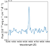 |
Fig. 1. Hα line of Gaia18cjb from LT SPRAT spectrum. |
2.2.2. LBT LUCI
We observed Gaia18cjb at the Large Binocular Telescope (LBT Observatory, Arizona) with LUCI1 and LUCI2 intruments in the zJ and HK filters on 2021 January 17. We reduced the data by using the SIPGI pipeline (Gargiulo et al. 2022), following the recipes indicated in the SIPGI documentation6 for the flat field correction, sky subtraction, wavelength calibration, and telluric correction. We then averaged the LUCI1 and LUCI2 spectra, to maximize the signal-to-noise ratio (S/N). Since we do not have contemporary zJHK photometry, we flux-calibrated the spectrum using SOFI continuum as both optical and NIR light curves suggest that the photometry does not vary much (e.g., Δmr = 0.2 mag and ΔmW1 = 0.1 mag) between January and May 2021 (see Fig. 2).
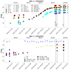 |
Fig. 2. Visible (top) and IR (bottom) light curves of Gaia18cjb. The red circle highlights the Gaia Alert trigger. The error bars smaller than the symbol size are not presented. Grey dashed lines correspond to the epochs for which we collected NIR spectroscopy. |
2.2.3. NTT SOFI
The blue part (0.95–1.64 μm) of the NTT/SOFI spectrum was observed on the 2021 May 5 and 8, while the red part (1.53–2.52 μm) only on the 8th. For the observed data, flat-fielding, bad pixel removal, sky subtraction, aperture tracing, and wavelength calibration were applied with the Image Reduction and Analysis Facility (IRAF, Tody 1993). For the wavelength calibration, a Xenon spectrum was used. The hydrogen lines in the telluric standard stars were removed by Gaussian fitting. The spectra were flux calibrated using the contemporary photometry (see Sect. 2.1). Technical details are reported in Table 2 and the spectra are presented in Sect. 3.
2.2.4. GTC EMIR
We obtained JHK-band spectroscopy of Gaia18cjb with the GTC/EMIR medium-resolution multi-object spectrograph (Espectrógrafo Multiobjeto Infra-Rojo, Garzón et al. 2022) in long slit mode on 2022 October 26. EMIR is equipped with a 2048 × 2048 Teledyne HAWAII-2 HgCdTe NIR-optimised chip with a pixel size of 0.2″. The total exposure time on source was 1920 seconds per grism. One grism per each band (J, H and K) was used. A typical ABBA nodding pattern was applied. The seeing during the observations was FWHM ∼ 1.2″.
The spectra were reduced using several python routines customised by GTC staff for EMIR spectroscopic data. The sky background was first eliminated using consecutive A-B pairs. They were subsequently flat-fielded, calibrated in wavelength and combined to obtain the final spectrum. To correct for telluric absorption, we observed a telluric standard star with the same observing set up as the science target, right after the Gaia18cjb observations and at similar airmass. To apply the correction, we used a version of Xtellcor (Vacca et al. 2003) specifically modified to account for the atmospheric conditions of La Palma observatory (Ramos Almeida et al. 2009). We calibrated the flux scale of GTC spectra using the GTC contemporary photometry, see Sect. 2.1.2.
3. Results
Our photometric results, used for the optical and IR light curves (see Sect. 3.1), are shown in Appendix A. Uncertainties are computed as the quadratic sum of the uncertainty of the aperture photometry, the scatter of the individual exposures, and the uncertainty of the photometric calibration. Normalized and flux calibrated spectra are presented in Sect. 3.4 and Appendix B, respectively. They show emission lines typical of YSOs such as magnetospheric accretion features (HI), winds and outflows (H2), and CO/NaI from the disk.
3.1. Light curves
Figure 2 shows the optical (top panel) and IR (bottom panel) light curve of Gaia18cjb.
3.1.1. Optical light curve
The optical light curve shows the Gaia G-band brightening event of about 4.6 mag from 2015 February to 2020 May (black stars). Afterwards, the brightness still increased, albeit more slowly, by only 0.3 mag, up to the last epoch in March 2023. The overall brightening in the Gaia light curve is of about 4.9 mag. The outburst is still ongoing and there is no indication that the peak of the outburst has been reached. However, it looks as though Gaia18cjb reached a constant plateau in 2022-23. The photometric data, collected from other observatories after 2016, cover timescales shorter than Gaia. They confirm the brightening and the current “plateau” phase. Indeed, the r-band data (orange stars, filled circles, triangles, diamonds, and crosses, depending on the telescope) show a strong increase of brightness consistent with the Gaia data acquired with the G filter. The variability within 13 years is ∼5.0 mag, a typical value for FUors variability (Fischer et al. 2022). However, the rise time (several years) is atypical for these kinds of objects, although there are FUors-like objects whose light curve has been increased for decades (e.g., V1515 Cyg, Hartmann & Kenyon 1996; Szabó et al. 2022). The ZTF g-band shows brightening of 2.8 mag within 4.75 years, and only of 0.5 mag after 2021 January (LUCI Epoch). NTT, RC80, Suhora, and ADYU60 light curves are in agreement within each other when the filter is the same and confirm the fact that since 2020 May the brightness of Gaia18cjb is still increasing but with a smaller amplitude than before (about 0.1 mag) in the i-, r-, V-, g-, and B- bands.
PanSTaRRS monitored Gaia18cjb prior to Gaia in the g, r, and i bands from 2010 to 2013. During these years the variation in the r band is only 0.65 mag, suggesting a quiescent phase before the ongoing outburst. The same behavior is also seen in other bands. We note that the last data points from the PanSTaRRs r band are brighter than the first data points of Gaia, suggesting the presence of some possible pre-burst variability. We also note that PanSTaRRS r and g variability is greater in a specific epoch (i.e., May 2012) than in the three years overall. This can be a hint of ordinary small-amplitude accretion events as seen in CTTSs (see e.g., Fischer et al. 2022, and references therein).
3.1.2. IR light curve
We studied the variability also in the IR using WISE, UKIDSS, and PanSTaRRS archival data together with our acquired photometry (bottom panel of Fig. 2). The W1 channel at 3.4 μm (yellow filled dots) varies by 0.6 mag, while the variability is only 0.4 mag at 4.6 μm (W2 channel, blue dots) from 2010 March to 2022 October. The variability of both W1 and W2 channels reduced down to 0.1 since 2021 January. The W2 variability does not seem to follow the variability we see in the optical bands and it hovers around a mean value between the pre-burst phase and the burst phase. We cannot confirm this trend in the W1 band since there were no W1 observations in the pre-burst phase. The IR light curve is similar to V1057 Cyg, one of the classical FUors (Szabó et al. 2021) post-1995, in displaying some kind of minor modulation.
The variability in the near-IR between UKIDSS (2007 April) and SOFI (2021 May) observations decreases with increasing wavelength: 2.70 mag, 2.14 mag, and 1.35 mag in J, H, and K bands, respectively. Interestingly, PanSTaRRS light curves, observed from 2010 to 2014, invert the trend: in the Y band the variability is larger (0.89 mag) than in the z band (0.39 mag). This can be explained by the large variability in the first epoch (2010 February), which may be due to the presence of a small burst or to a sudden increase of the light curve, as is often the case before a strong FUor-like burst (Audard et al. 2014). However, this could also be the result of the different sampling for the PanSTaRRS filters and, in turn, not necessarily associated with the intrinsic variability of the star.
We highlight that the photometric variability in the IR is moderate in general and it does not reflect the strong burst we observe in the visible. Indeed, the IR variability is as small as in typical non eruptive sources (see, e.g., Lorenzetti et al. 2012; Zsidi et al. 2022; Fiorellino et al. 2022). However, this result is puzzling since it suggests that the burst is restricted to the star and its immediate circumstellar environment and does not affect the dusty disk at all. We discuss possible interpretations of this result in Sect. 4.
3.2. Color-magnitude diagrams
To investigate the photometric properties of Gaia18cjb in the visible and IR bands, we built color-magnitude diagrams (shown in Fig. 3). The top-left panel corresponds to the g′ versus g′−r′ diagram. It shows extinction related to color variations and a linear decreasing trend. This trend suggests that g′- and r′-band variations are correlated, but the g′-band variation is larger than r′-band variations (see light curves in Fig. 2). A similar trend is also present in the IR color-magnitude diagram in the bottom-right panel, where W1 and W1–W2 are strongly correlated following the direction of the reddening vectors. It appears that the source is redder when fainter, hence, the downward trend in the color-magnitude diagram. The top-right panel and the bottom-left panel present the V-band photometry versus V − i′ and V − r′, respectively. In both cases, the distribution appears to be vertical, suggesting that the variability amplitude is similar in the V and i′ and in the V and r′ bands. In all the color-magnitude diagrams in Fig. 3 we note a temporal trend: the variation of the colors decreases with time as the source brightens. This produces a trend on the opposite direction of the reddending vectors. In general, the difference between the reddening law with RV = 3.1 (black arrow) and RV = 5.5 (red arrow) is small, and it is hard to distinguish which one of the two is followed better from the data points. In the g versus g − r plot this difference is more evident and the black arrow better reproduces the variation of extinction from 2018 to 2020 (orange-blue filled dots), while the steeper slope of the red arrow better reproduces AV variations in the quiescent phase and in the latest epochs (from 2021 onward, yellow-blue filled dots). We discuss possible interpretations of this result in Sect. 4.
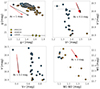 |
Fig. 3. Color-magnitude diagrams of Gaia18cjb based on data from Pan-STARRS data (yellow filled circles), ZTF, Konkoly, Mt Suhors, and WISE data before LUCI epoch (orange filled circles), and after LUCI epoch (blue filled circles). The arrows show the reddening vector, assuming extinction law from Cardelli et al. (1989) with RV = 3.1 (black arrow) and RV = 5.5 (red arrow), respectively. |
Figure 4 shows the J − H vs. H − K diagram, which can be used to classify a YSO and to estimate its extinction. We used UKIDSS and 2MASS archival data and the newly acquired SOFI and GTC data points. In the same figure, we plot the giant branch (GB) locus (green dot-dashed line), zero age main sequence (ZAMS, orange line), and classical T Tauri Stars (CTTS) locus (Meyer et al. 1997), where CTTS are not extincted (AV = 0 mag, blue dashed line). By following the extinction vector by Cardelli et al. (1989) and RV = 3.1 (black arrow), it is possible to compute the extinction of a CTTS. The 2MASS and UKIDSS data of Gaia18cjb lie within the CTTS locus, suggesting negligible extinction, while recent data points lie below the CTTS locus, making not possible to compute its extinction with this method and suggesting that Gaia18cjb is less evolved than a typical CTTS. However, in the case of GTC data, considering the error bars, it is possible that the Gaia18cjb colors lie on the CTTS locus, suggesting low extinction. This movement along the CTTS locus from redder to bluer is similar to what was found in Kóspál et al. (2011, see Fig. 7 therein) for HBC 722. In general, it is known that highly accreting stars become bluer in burst with respect to quiescence (see e.g., Lorenzetti et al. 2007, 2011; Hillenbrand et al. 2018; Szegedi-Elek et al. 2020), suggesting an accreting nature for Gaia18cjb.
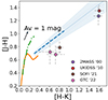 |
Fig. 4. NIR color-color diagram of Gaia18cjb. Purple and red circles are pre-outburst data from 2MASS and UKIDSS observations in 2000 and 2010, respectively, while the brown and pink dots correspond to SOFI and GTC photometry in the burst phase (2021 and 2022, respectively). The blue dashed line and light blue region represent the CTTS locus and its uncertainty (Meyer et al. 1997), and the tiny blue dotted line its extension toward larger color indices. The orange solid and green dotted-dashed lines correspond to the colors of ZAMS and GB stars, respectively. The black arrow shows the reddening vector for a source with 1 mag of extinction (Cardelli et al. 1989, RV = 3.1). |
3.3. Spectral energy distribution
From an observational point of view, YSOs are usually classified on the basis of their spectral energy distribution (SED, Lada & Wilking 1984; Lada et al. 1987; André 1995; Greene et al. 1994). Figure 5 shows the SED of Gaia18cjb, in the low brightening state (dots, before 2020), resembling the SED of an embedded object as a Class I YSOs, and in the outburst state (after 2020, star symbols), which is similar to a flat spectrum source. The data we used to build up the SEDs were observed at different periods and are listed in Appendix A.
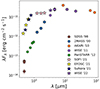 |
Fig. 5. Spectral energy distribution. Circles and stars are observations taken before and after 2020, respectively. |
We note that, based on the light curve, it is challenging to determine when the outburst begun. The Gaia alert was triggered in 2018, but the luminosity had already increased since 2015 (when first Gaia data are available), while the PanSTARRS monitoring between 2010 and 2014 does not provide definitive conclusions about the quiescent phase of this object, even if we can tentatively assume the average PanSTARRS magnitudes as values for the quiescent phase (mg = 21.8 ± 0.4, mr = 20.0 ± 0.2, mi = 19.1 ± 0.1, mz = 18.5 ± 0.1, and mY = 18.2 ± 0.2). However, we distinguish here between the first part of the optical light curve, where the luminosity increases by 4.6 mag over about 10 years, and the second part, after the LUCI epoch, where the luminosity moderately increases by only 0.3 mag in three years (see the top panel of Fig. 2 and Sect. 3.1). We refer to the first one as the “brightening” or “low-state” phase and to the latter one as the “bursting” or “high-state” phase. We stress that this nomenclature is only useful to distinguish between the amplitude in the variability while in both the phases the burst is on, with the luminosity increasing.
We computed the spectral index  between 2.16 μm and 22.1 μm using 2MASS and WISE data, respectively. For the pre-outburst phase, we obtain α = 0.55 ± 0.28, which classifies Gaia18cjb as a Class I protostar (α > 0.3). We note that the spectral index is also compatible with a flat spectrum object (−0.3 < α < 0.3) within the error. We conclude that Gaia18cjb is most likely a Class I YSOs, with a small chance that it is a flat spectrum. We also note that the classification we use computes the spectral index using λFλ at 2 μm and 24 μm (not 22 μm as we do), but based on the SED shape, we do not expect a large difference between the flux at 22 μm and at 24 μm.
We also computed the spectral index using SOFI K-band and WISE W4 data to get an estimate of α for the eruptive phase. SOFI observations were taken during the eruptive phase, while WISE observations are not, but since the low variability at long wavelengths and the lack of observations around 20 μm during the outburst, we used the same value as before (when considering the brightening SED). We obtained: α = 0.09 ± 0.02, which is compatible with a flat spectrum.
In both the low level and high level phases, the spectral index we compute does not describe Gaia18cjb as a Class II PMS young star. In the scenario where the empirical classification of YSOs based on the SED spectral index corresponds to an evolutionary classification, Gaia18cjb seems to be in between the protostellar phase, where the star is embedded in its envelope and the accretion is very high (Class 0 and I YSOs), and the pre-MS phase, where most of the stellar mass is accessed and the star is approaching the ZAMS (Class II and III YSOs). Estimates of Class 0 lifetimes are between 0.2 and 0.6 Myr, whereas based on Spitzer timescales, we see lifetimes of Class I and flat spectrum YSOs are 0.54 Myr and 0.40 Myr, respectively (Evans et al. 2009). Therefore, if the classification based on SED spectral index corresponds to evolutionary stages and our classification is correct, we can assume an age of about 1 Myr for Gaia18cjb.
3.4. Emission lines
The spectra of young solar-type stars show many features tracing the star-disk interaction as, for example, accretion and/or ejection. Our NIR spectra of Gaia18cjb covers several emission lines and, in particular, some accretion tracers, such as Brγ and Paβ. We describe here how we have measured the fluxes of these lines to be used for the analysis.
We measured the equivalent width (Weq) and the observed line flux (Fobs) from the normalized and flux calibrated spectra, respectively, as follows. We fitted a linear curve to the local continuum in a wavelength range of Δλ = 2 nm, centered on the emission line wavelength λ0. We slightly modified this range (when needed), taking the one most suitable for each line; for example, by avoiding other emission lines (if present) or telluric absorption lines. The line flux was determined by subtracting the local continuum from the spectra and integrating it over the line. We computed the noise of the line by multiplying the standard deviation of the local continuum (rms) for the wavelength element between two pixels, Δλ, and multiplying this by the square root of the number of pixels within the wavelength range (Npix). We considered a line to be detected when its S/N > 3. For those lines that were detected in at least one epoch, we estimated the upper limits in the other epochs as three times the noise:
 (1)
(1)
For LUCI spectra, the flux calibration with contemporary photometry was not possible. Therefore, we computed the observed flux by multiplying the equivalent width of each line by its local continuum in the SOFI spectrum. We stress that the acquisition of the LUCI spectrum was contemporaneous to that of the SOFI data. Equivalent widths and fluxes are reported in Tables 3 and 4, respectively.
Equivalent width of Gaia18cjb emission lines for the three epochs we observed.
Observed fluxes of the emission lines in the Gaia18cjb spectra.
LBT spectrum: 2021 January. Figure 6 reports the LBT normalized spectrum and the emission lines detected. This spectrum shows several accretion tracers such as Paβ, Paγ, Paδ, Brγ, Br10, Br11, Br12, Br13, Br14, and the Na I doublet. The H2 line in emission suggests the presence of some shocked material in ejection, as winds. We also detected Fe I in the emission.
SOFI spectrum: 2021 May. Figure 7 shows the SOFI normalized spectrum. It confirms the presence of accretion (Paβ, Paγ, Brγ, Br16, Br18, Na I doublet) and ejection (H2) tracers. Emission lines of Mg I and Ca I were also detected.
GTC spectrum: 2022 October. The GTC spectrum shows up to 9 lines of the Brackett series, but, due to the restricted wavelength range in the blue part of the spectrum, only the brightest line of the Paschen series (Paβ see Fig. 8). Then, Fe I, Mg I, Ca I, and Na I lines were detected, while H2 emission was confirmed.
4. Discussion
In this section, we discuss evidences supporting that Gaia18cjb is a YSO and put its accretion properties into context with respect to other erupting YSOs.
4.1. On the distance of Gaia18cjb
Measuring the distance of an unknown object is a complex task. In particular, the case of Gaia18cjb presents its own set of challenges, given the large parallax uncertainty derived by Gaia. In this section, we discuss strengths and limitations of the photogeometric distance by Bailer-Jones et al. (2021).
The Gaia DR3 parallax for Gaia18cjb is p = 0.83 ± 0.69 mas. With such a large uncertainty, the parallax method does not yield accurate results. Indeed, the main DR3 catalog does not provide a distance for sources whose parallax has a low S/N, including our target. For this reason, Bailer-Jones et al. (2021) developed a probabilistic approach to estimate stellar distances. This method relies on the prior using a full range of populations in the mock catalogue, based on the Besancon Galaxy model. For each source, they computed two posterior probability distributions over distance: a geometric distance, based only on the prior and the parallax, and the photogeometric distance, based also on the G magnitude and the BP−RP color. Gaia18cjb’s geometrical distance is  kpc, while the photogeometrical distance is
  kpc. The recommendation of Bailer-Jones et al. (2021) is to adopt the photogeometric distance for sources whose parallax has a low S/N. This is the case of Gaia18cjb.
The point of the distance inference in Bailer-Jones et al. (2021) is to provide a gradual transition from data-dominated to prior-dominated distance estimates. While the populations used by Bailer-Jones et al. (2021) contained YSOs, their results are not optimized for intrinsically red sources with high circumstellar extinction, such as YSOs. While a more appropriate photometric prior constructed solely for young stars would provide more accurate photometric distances, this is not the primary objective of our study. With the aim of remaining conservative, we discuss how our main results change, considering the spread in the distance suggested from Gaia parallax d ∼ 1/p = 660 pc − 7140 pc. In the following, we discuss results assuming dmin = 660 pc, dBJ = 1030 pc, and dmax = 7140 pc.
4.1.1. Interstellar extinction
To compute the reddening of Gaia18cjb due to the interstellar extinction, we used the 3D dust maps based on Gaia parallaxes and stellar photometry from Pan-STaRRS 1 and 2MASS (Green et al. 2019). We ran the dustmaps python package7, using the most updated version Bayestar 2019, assuming RV = 3.1, and the reddening law by Cardelli et al. (1989). We performed the same exercise using the STructuring by Inversion the Local Interstellar Medium (STILIsM, Capitanio et al. 2017; Lallement et al. 2018) with the online tool8. In both cases, we consider these values as lower limits for the extinction towards the source, because they are values averaged in a certain area and, most importantly, not sensitive to local circumstellar extinction. We repeate the calculation for dmin, dBJ, and dmax. In Table 5AV results are listed, ranging from 0.4 mag to 3.0 mag depending on the distance. We note that extinction estimates obtained with STILIsM show slightly higher values, but compatible within the errors.
Interstellar extinction and bolometric luminosity at different distances.
4.1.2. Bolometric luminosity
Using the fluxes reported in Appendix A, we computed the bolometric luminosity by integrating the SED fluxes (Fλ) with a dedicated python procedure, following the same method already used in literature (e.g., Antoniucci et al. 2008; Fiorellino et al. 2021, 2023). We integrated the SED from the shortest wavelength, interpolating with straight lines in the log λ − log Fλ plane between the available SED points. We denote the value found with this method as  to highlight that this is the bolometric luminosity corresponding to the pre-burst phase, obtained using the photometry observed before 2015 (filled circles in Fig. 5).
We added optical and NIR photometry acquired during the outburst (i.e., after 2015, filled stars). For the high-level phase, we computed the bolometric luminosity using Suhora, NTT/EFOSC, NTT/SOFI, and W1 photometry (blue, yellow, pink, and purple stars in the figure) instead of SDSS, PanSTARR, and 2MASS photometry (brown, green, and blue filled circles in the figure). As there is little or no variability in W2, we assumed that the source was constant within about 0.4 mag at 4.5 μm and we used the ALLWISE and AKARI points reward these wavelengths for the outburst SED, too. We name the value found with this method  , to highlight that this is the bolometric luminosity computed using the photometry observed during the ourtburst (see Fig. 5).
To build the SED and to measure the bolometric luminosity of Gaia18cjb we used the observed fluxes that were not corrected for extinction. We note that the longest wavelength data point we have is AKARI at 90 μm, and we assume a decrease in the emission as 1/λ2 after that. Even after applying this correction, we are aware that the bolometric luminosity derived so can be underestimated due to the lack of information at longer wavelengths. We also assume that beyond 3.6 μm the SED did not change during the burst.
It is desirable to correct the flux for extinction and compute the bolometric luminosity corrected for the extinction ( ). Following Evans et al. (2009), since the spectral index suggest Gaia18cjb can be classified as a Class I/flat spectrum YSO, we used the interstellar AV to remove foreground extinction, but not local extinction from the surrounding envelope, which will be reradiated in the FIR. We used the mean value between the values we obtain with the dustmaps and STILIsM softwares. Results are listed in Table 5.
The lowest possible distance and the BJ distance both results in pre-outburst luminosities (1.4 − 3.5 L⊙) typical of a low-mass young protostar, and the outburst luminosities (3.1 − 8.3 L⊙) are reasonable for modest accretion outbursts (cf. HBC 722 or some EXors). The luminosities obtained with the largest possible distance are in the several hundred L⊙ range both in quiescence (173 L⊙) and in outburst (534 L⊙). While such a large outburst luminosity is possible in some of the most luminous and most highly accreting FUors (e.g., V1057 Cyg or FU Ori; Audard et al. 2014, and references therein), the quiescence luminosity is definitely too high for a low-mass YSO.
4.1.3. Stellar parameters and accretion rates
In this section, the stellar parameters (spectral type, extinction, luminosity, radius, and mass) and accretion properties (accretion luminosity and accretion rate) of Gaia18cjb are determined.
An estimate of the total extinction can be done by assuming that the accretion luminosity, Lacc, as derived from different accretion tracers, is the same. In order to derive Lacc, we used the Paβ and Brγ lines and the empirical relationships between Lacc and the line luminosity, Lline, by Alcalá et al. (2017). By minimizing the quantity |Lacc(Paβ)−Lacc(Brγ)| it is possible to estimate the circumstellar extinction, AV, as follows: the observed fluxes of the Paβ and Brγ lines were dereddened with a series of AV values ranging from 0 to 200 mag in steps of 0.1 mag. The AV values minimizing the |Lacc(Paβ)−Lacc(Brγ)| quantity are given in Table 6 and shown graphically in Fig. 9. For these, we determined values of log(Lacc/L⊙) between −0.07 and 2.63 dex, depending on the chosen distance (see Table 6). A robust value of AV for the eruptive phase can be then obtained by computing the average from the three individual estimates, the standard deviation being the error. This value ranges from AV = 10.5 ± 2.7 mag to AV = 15.0 ± 0.3 mag, depending on the distance (see Table 6).
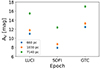 |
Fig. 9. Extinction estimates of Gaia18cjb computed from the empirical relations between the accretion luminosity and Brγ and Paβ lines. Different colors represent AV estimates at different distances as described in the legend. |
Circumstellar extinction and accretion luminosity estimates for Gaia18cjb using empirical relations from Alcalá et al. (2017).
Assuming that Lbol = L⋆ + Lacc, we get a rough estimate of the stellar luminosity for Gaia18cjb by knowing the dereddened bolometric luminosity for the eruptive phase,  , and the accretion luminosity, Lacc. We thus obtain L⋆ = 1.9 ± 1.2 L⊙ for a dmin = 660 pc, L⋆ = 6.0 ± 1.2 L⊙ for dBJ = 1030 pc, and L⋆ = 107 ± 62 L⊙ for dmax = 7140 pc.
Based on the spectral features, we discard the possibility for Gaia18cjb to be a high-mass star, since high excitation lines, such as He I are not detected. The stellar luminosity we obtain if assuming a distance of 7140 pc (L⋆ = 107 ± 62 L⊙) is, therefore, not compatible with information contained in our spectra. Our spectra also discarded the possibility that the spectral type of Gaia18cjb could be later than K7. Indeed, M-type and later type sperctra show photospheric absorption features such as the CO and VO bands. It is plausible to argue that the molecular bands could be veiled by the strong continuum emission; however, if that were the case, then the accretion luminosity should be extremely high – but the Weq value we obtained suggests this is not the case.
Then, we used the evolutionary tracks by Siess et al. (2000), assuming an age of ∼1 Myr (see Sect. 3.3) and considering only spectral type earlier than K7. We found that our results for L⋆ at 660 pc are compatible with a young star with stellar mass of M⋆ = (0.7 − 1.6) M⊙, a radius of R⋆ = (3.5 − 1.4) R⊙, and Teff = 4000 − 4600 K, corresponding to SpT = K7–K3. The same exercise for L⋆ at 1030 pc leads to a young star with stellar mass of M⋆ = (0.7 − 2.2) M⊙, radius of R⋆ = (4.4 − 2.6) R⊙, and Teff = 4000 − 5080 K, corresponding to SpT = K1–K7.
From the derived Lacc and stellar parameters, we computed the mass accretion rate (Ṁacc) in the bursting phase using the relation from Hartmann et al. (1998) in the framework of magnetospheric accretion scenario:
 (2)
(2)
where Rin is the inner-disk radius which we assume to be Rin ∼ 5R⋆ as discussed by Hartmann et al. (2016, see their Eq. (3)) and for consistency with previous similar studies (e.g., Park et al. 2022; Cruz-Sáenz de Miera et al. 2022, 2023). We obtained Ṁacc = 1.8 × 10⁻⁷ 1.6 × 10⁻⁷ M⊙ yr−1, for dmin; and Ṁacc = 1.0 − 5.3 × 10⁻⁷ M⊙ yr−1, for dBJ. Both the estimates are similar to the values found in highly accreting CTTSs and in EXors-like objects (e.g., Giannini et al. 2022).
4.2. On the YSO Nature of Gaia18cjb
Besides the photometric and spectroscopic features presented in the previous sections, another important aspect supporting the PMS nature of Gaia18cjb is the enviroment in which the object is located. We investigated the region nearby Gaia18cjb looking for its possible association with a star-forming region. Figure 10 shows the environment in the general direction of Gaia18cjb, with the nearby known star-forming regions highlighted. Gaia18cjb is located three degrees south-west of the Rosette star-forming region in the Monoceros constellation. Three degrees angular distance corresponds to ∼50 pc at 1 kp. The distance to the Rosette complex is 1489 ± 32 pc (Mužić et al. 2022). Thus, it is unlikely that Gaia18cjb is connected with the Rosette star-forming region if its distance is d ≤ dBJ. In contrast, if Gaia18cjb distance is similar to the Rosette star-forming region, then it might be part of the star-forming complex. The VDB 85 cluster is about ∼1.5 degrees away from Gaia18cjb and its measured distance is about ∼1.69 kpc (Cantat-Gaudin & Anders 2020), so, for the same reasoning applied to the Rosetta Complex, it is unlikely for Gaia18cjb to belong to this cluster. According to the 3D extinction map STILIsM, in correspondence of the TGU 1475 dark cloud position (l, b = 210.87°, −3.28°), there is one dark cloud at a distance of ∼0.9 − 1.0 kpc, which we may suspect that corresponds to TGU 1475. The ellipse in Fig. 10 shows its nominal size from Dobashi et al. (2005). Although TGU 1475 and Gaia18cjb could have similar distances based on the assumption that d ≤ dBJ, in looking at Fig. 10, we note that our target is outside the dark cloud. Therefore, we may conclude that Gaia18cjb is not a member of any of the known star-forming regions.
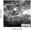 |
Fig. 10. Background of the figure is the Planck 857 GHz map, 10 degrees in size, centred on Gaia18cjb, the red star symbol in the plot. Blue and orange dots are sources with Hα-excess from Fratta et al. (2021) whose distances are 0.95 pc < d < 1.05 pc. The orange dots are sources whose proper motions are within 3 mas yr−1 from Gaia18cjb proper motions (see Fig. 11). The regions closes to Gaia18cjb are highlighted. |
Recent investigations (Fratta et al. 2021; Prisinzano et al. 2022), based on Hα surveys and on Gaia DR3, have shown evidence of populations of YSO candidates distributed in large volumes around the previously known star-forming regions. We consider whether Gaia18cjb might be part of such population in the general area of Monoceros. The sources showing Hα−excess are overplotted in Fig. 10, based on the areas selected by Fratta et al. (2021) and whose Gaia distance is between 0.95 kpc and 1.05 kpc, similar to the Gaia18cjb distance proposed by Bailer-Jones et al. (2021). The lack of Hα emitting objects in the southern part is due to the latitude limit of the INT Photometric Hα Survey of the north Galactic plane, IPHAS. We also distinguish in this plot objects having proper motions consistent, within 3σ, to the proper motion of Gaia18cjb (orange dots) and those with inconsistent with proper motion (blue dots). These two samples are also plotted in the proper motion diagram in Fig. 11 (right panel). Gaia18cjb, shown as a red star symbol in the figure, is not associated with any source in this catalog.
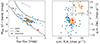 |
Fig. 11. Analysis on the young stellar nature of Gaia18cjb. Left: color-absolute magnitude diagram not corrected for the extinction. The red star symbol corresponds to Gaia18cjb. The black solid and dashed lines show the ZAMS and the 1 Myr isochrone, respectively (Dell’Omodarme & Valle 2013). Dots are sources which show Hα-excess from Fratta et al. (2021) catalog whose distance is 0.95 kpc < d < 1.05 kpc. Orange dots are sources with proper motions consistent within 3σ the propoer motion of Gaia18cjb (see right panel). The error bars smaller than the symbol size are not presented. The purple arrow represents an extinction vector of 1 mag. However, the AV vector depends on the color index and on the position in the diagram; see Prisinzano et al. (2022). Right: proper motions diagram of the Hα-excess sample. Symbols are the same as in the left panel. |
Figure 11 (left panel) shows a color-magnitude diagram of the sample with Hα excess, where the absolute magnitude computed from the Gaia G band as a function of the GBP − GRP color (blue and orange colors are as in Fig. 10). The black lines correspond to the ZAMS (solid) and to the 1 Myr isochrone (dashed, see Dell’Omodarme & Valle 2013; Randich et al. 2018; Tognelli et al. 2018, 2020). Models have been converted into the Gaia observed plane using the recent EDR3 filters passbands9 with the MARCS 2008 (Gustafsson et al. 2008) synthetic spectra for Teff ≤ 8000 K and Castelli & Kurucz (2003) spectra for higher Teff (see e.g., Prisinzano et al. 2022). About 97% (91/94) of the Hα-excess sample lie above the ZAMS (blue dots), while only three lie below the ZAMS line. However, many of these objects, in particular, those piled-up close to the ZAMS, may be evolved Hα emitting stars, such as novae and symbiotic stars (see Munari et al. 2022). We note, however, that symbiotic stars have giant companions and so are located near the giant sequence and quiescent novae resemble nova-like cataclismatic variables which lie between white dwarf and MS phases (see, e.g., Merc et al. 2020). Classical novae in outburst would probably be much brighter than the MS. We note that basically all the objects with proper motion compatible with those of Gaia18cjb (orange dots) lie well above the ZAMS hence, it is likely they are pre-MS (PMS) stars. However, wide-band spectroscopy of these objects is necessary to definitely establish their evolutionary status.
The red star symbol lying immediately above the ZAMS corresponds to the Gaia18cjb mean values of absolute magnitude and GBP − GRP color provided by the Gaia archive: G = 19.751 ± 0.010 mag, GBP = 20.65 ± 0.77 mag, and GRP = 18.16 ± 0.77 mag. These values, reported in Gaia EDR3 are averaged on the period 2014 July to 2017 May, when Gaia18cjb had already started brightening, but was still relatively faint; thus, it is more likely to display quiescent than outburst properties. We stress that the magnitudes of all these sources are not dereddened, implying that after correcting each source for its extinction, they will move up and left in the color-magnitude diagram. With respect to Gaia18cjb, we estimated an accretion luminosity in burst which is about 27% of the bolometric luminosity and AV ∼ 8 − 12 mag. With these values, the contribution of the extinction is larger than the contribution of the accretion, ending up moving Gaia18cjb up in the Mabs versus GBP − GRP plot. Therefore, we can speculate that these sources lie above the ZAMS, and are young stars. The study of the spatial distribution of YSO candidates within 1.5 kpc by Prisinzano et al. (2022), based on Gaia DR3, highlighted a population of distributed YSO candidates surrounding the previously known star-forming regions in the Monoceros region, but Gaia18cjb was not selected by their criterion, probably because it was too faint to be included in their catalog.
In summary, we selected 20 emission line stars (19 + Gaia18cjb) that: 1) lie above the ZAMS in the Gaia color-magnitude diagram; 2) are located at approximately the same distance (0.95 kpc < d < 1.5 kpc); and 3) have coherent proper motion. We therefore conclude that these likely YSOs, including Gaia18cjb might be part of the distributed population of the Monoceros complex. This results may indicate that the dBJ could be a good estimate of the real distance of Gaia18cjb. However, as discussed in Sect. 4.1, the photogeometric distance dBJ may be strongly affected by the prior for the absolute G-band mag, being dominated by the sample of MS stars.
Several pieces of evidence suggest that Gaia18cjb is a young star, based on: (i) the high probability of Gaia18cjb to be a YSO: 83%, computed by Marton et al. (2019; ii) the similarity between Gaia18cjb SED and the SED of a young accreting object (Fig. 5); (iii) the spectral index which classifies Gaia18cjb as Class I YSO during the pre-burst phase and as a flat spectrum YSO during the burst (Sect. 3.3); (iv) the detection of CTTSs typical features, as accretion and ejection tracers in the NIR spectra (see Sect. 3.4); and (v) the environment in which the object is projected on the sky. All these facts together lead us to conclude that Gaia18cjb is an accreting young star.
4.3. On the outburst of Gaia18cjb
The optical light curve (Fig. 2) presents a typical amplitude of a FUor-like object, on timescales that are compatible with EYOs, and longer than typical EXors and smaller than typical FUors. On the contrary, the WISE light curves in the MIR show no evidence of such FUor-like strong burst and the variability is smaller than expected for a FUor-like object, while it is compatible with the EXor-like YSOs or even CTTs variability.
If a burst is present, as the optical light curves suggest, it is not clear why it is less pronounced at NIR wavelengths and does not affect the SED at (and possibly beyond) the WISE band 2 (4.6 μm), since eruptive objects usually show similar variability at optical and IR wavelengths (see for example Gaia19fct, Park et al. 2022). Naively, we could conclude that the large optical and smaller amplitude in the IR for Gaia18cjb is due to variability in extinction. Looking at the color-magnitude diagrams in Fig. 3, we see that the extinction would only partially explain the variability of Gaia18cjb as well as its low-level and high-level colors.
For example, if the observed NIR variability (ΔW1 ∼ 0.6 mag, ΔmK ∼ 0.7 mag, ΔmH ∼ 2.2 mag, ΔmJ ∼ 2.9 mag) were caused only by extinction, this would correspond to a visible amplitude of ΔmV ∼ 10 − 12 mag, that is too large in comparison with the observed visual variability (Δmr ∼ 5 mag). This suggests that at least some of the observed blueing is intrinsic and not just linked to reddening. On the other hand, the accretion burst has to be relatively mild, as the continuum at 4.6 μm is barely or not affected at all. It is thus possible that the observed photometric variability of Gaia18cjb is a combination of enhanced accretion and reduced extinction, as inferred in Gaia19ajj (Hillenbrand et al. 2019). The reduced extinction might possibly rise from winds triggered by the enhanced accretion. These would partially clear the dust in the outflow cavities. This scenario is compatible with the H2 line seen during the burst (see Sect. 3.4).
The burst weakness is also supported by the analysis of the spectra. The latter do not show typical FUors-like features such as the triangular shape in the H band or the undetected NIR HI and CO lines in absorption (Greene et al. 2008). On the contrary, accretion tracers are detected in emission in all the epochs we investigated, confirming this source is an accreting young star and strengthening the EXor nature of Gaia18cjb burst.
In Sect. 4.1.3, using empirical relations, we report that Lacc ranges from 0.85 L⊙ to 2.24 L⊙, while Ṁacc ranges from 2.8 × 10⁻⁸ M⊙ yr−1 to 1.0 × 10⁻⁷ M⊙ yr−1 if dmin ≤ d ≤ dBJ.
Calculating Lacc using empirical relationships from Alcalá et al. (2017) is an indirect method that has shown success with CTTSs; however, some evidence has recently emerged that it may not be always applicable to eruptive sources, even if we expect magnetospheric accretion, as would be the case for EXors objects. For instance, a recent analysis of EX Lupi revealed that several emission lines indicated lower values of Lacc compared to the slab model, the direct way to determine Lacc in the framework of magnetospheric accretion (Cruz-Sáenz de Miera et al. 2023). They suggested that this discrepancy may arise from the challenge of identifying the continuum in a highly accreting objects. To investigate whether this holds true for Gaia18cjb, we would require wide-band spectroscopic data covering the Balmer continuum and Balmer jump to apply a slab model fit. Since we lack such spectroscopic data and, conversely, since we can only calculate Lacc from the Paβ and Brγ lines in the NIR, the estimate of Lacc obtained from empirical relationships using these lines is currently the best estimate of Lacc. However, we emphasize that due to the likely overestimated value of Gaia18cjb’s stellar luminosity and the uncertainty on the distance, there is a high probability that the accretion luminosity exceeds Lacc = 2.24 L⊙. This needs to be tested through the direct measurement of Lacc by studying the Balmer continuum excess emission and Balmer jump, using wide-band spectra.
Figure 12 shows the Lacc vs. L⋆ (top panel) and Ṁacc vs. M⋆ (bottom panel) of Gaia18cjb at dmin = 660 pc and dBJ = 1.03 kpc (red star symbols), compared to EX Lup (black stars, quiescent value from Cruz-Sáenz de Miera et al. 2023, and burst value from Fischer et al. 2022) and typical distributions for CTTSs in Lupus (grey, Alcalá et al. 2017), and Class I+flat spectrum protostars (pink, Fiorellino et al. 2023).
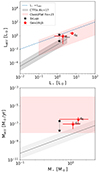 |
Fig. 12. Accretion parameters as a function of the stellar parameters. Top:Lacc − L⋆ diagram. The red and black star symbols correspond to Gaia18cjb and EX Lup, respectively. The blue dashed line represents the Lacc = L⋆ locus. The grey line is the best fit for the CTTSs of Lupus from Alcalá et al. (2017) and the grey region corresponds to the standard deviation of the t. Bottom: Ṁacc − M⋆ diagram. Star symbols are as in the top panel. The grey line is the best fit for the CTTSs of Lupus from Alcalá et al. (2017) and the grey region corresponds to the standard deviation of the t. The pink area corresponds to Ṁacc ranges for embedded Class I+flat spectrum YSOs from Fiorellino et al. (2023). |
The top panel of Fig. 12 shows that Gaia18cjb is located in the Class I+flat spectrum YSO parameter space, right below the Lacc = L⋆ threshold (dashed blue line). Therefore, during the epochs we investigated with spectroscopy (i.e., during the burst), the ratio between the stellar and the accretion luminosity was more similar to a YSO more evolved than a protostar if dmin ≤ d ≤ dBJ, and its accretion rate and stellar parameters are compatible with a Class I/flat spectrum object, suggesting Gaia18cjb’s evolutionary stage lies between the protostellar and the PMS phases. This in agreement with the flat spectrum classification suggested by the spectral index (Sect. 3.3). We note, however, that the luminosity of Gaia18cjb is still compatible with that of typical CTTS, if the distance dmin = 660 pc is adopted.
Regarding the Ṁacc versus M⋆ plot, the bottom panel of Fig. 12 shows that Gaia18cjb accretes more than typical CTTSs of the same stellar mass. Gaia18cjb location in this plot is in agreement with bright Class I and flat spectrum sources and the mass accretion rate is similar to what derived for EX Lup during the burst. Indeed, while the optical light curve resemble a FUor, the spectroscopic features and the accretion rate suggest an EXor-like nature of Gaia18cjb. Interestingly, there are at least two young stars, V350 Cep and V1647 Ori, displaying photometric characteristics of FUors in the visible bands and spectral characteristics of EXors (Herbig 2008; Ibryamov et al. 2014; Aspin & Reipurth 2009). In both cases, the conclusion was that the sources were probably intermediate objects between FUors and EXors.
The similarities between V350 Cep, V1647 Ori, and Gaia18cjb, might suggest that also Gaia18cjb is an intermediate object between FUors and EXors. However, there are a few aspects to take into account. First, V350 Cep and V1647 Ori also show P Cyg Hα profile, and random fluctuations in brightness with amplitudes of a few tenths of a magnitude in timescales of several days that we do not see in Gaia18cjb. Second, the current discussion about EYSs classification highlights that the classification in very tight containers (e.g., FUor, EXor, V1647 Or) is not sufficient. Gaia18cjb is another star suggesting instead a spectrum of classifications in the EYSs. Last, our results about accretion rates and stellar parameters should be considered as rough estimates, because our analysis is based only on NIR spectroscopy and because of the large uncertainty on the distance. To provide accurate parameters and hence, a robust characterization of Gaia18cjb, further observations and analysis are needed:
-
Continuing monitoring optical and IR light curves is crucial to follow the evolution of the Gaia18cjb burst. Also, JHK NIR IR monitoring is needed to study the light -curve variability in between the FUor-like visible light curve and the EXor-like IR light curves.
-
By having a flux-calibrated intermediate and high-resolution spectrum from the UVB to the NIR (as ESO/VLT XShooter can provide), we will be able to study the Li I (λ6708 Å) absorption line to reinforce the YSOs nature of Gaia18cjb, to perform a direct spectral typing and determine in a more accurate way the stellar parameters, and hence, measure the accretion luminosity from the Balmer continuum excess emission. As a consequence, we will be able to provide robust estimates of the stellar and accretion parameters and of the mass accretion rate.
-
Millimeter interferometry will provide estimates for disk mass and radius which are needed to prove the instability of the disk and believed to trigger the eruptive accretion.
-
Accurate distance estimate, by using a pre-MS-dominated prior in the Bailer-Jones et al. (2021) prescription or a more accurate parallax estimate from GDR4.
5. Conclusions
The goal of this discovery paper is to determine the nature of the Gaia-alerted object Gaia18cjb. For this purpose, we collected all the available photometry in the archives and monitored Gaia18cjb in optical bands. NIR spectroscopy was also performed in three epochs between 2020 and 2022 and we studied the object’s variability, stellar and accretion parameters, and inspected the sky region nearby Gaia18cjb.
The large uncertainty on the Gaia parallax and the MS-dominated prior of the Bailer-Jones et al. (2021) method, prevented us from adopting a precise distance for this source. Because of this, we cannot derive precise values, but only ranges for the stellar and accretion parameters based on the comparison between analytical results and spectral features. Comparing the Gaia stellar parameters and accretion rates with those of CTTSs, protostars, FUors, and other similar eruptive objects as EX Lup, V350 Cep, V1647 Ori, and Gaia19ajj, our results suggest Gaia18cjb is a young star experiencing eruptive accretion. It can be classified as in between FUors and EXors, namely: the length of the burst points to a FUor-like nature, whereas the strength of the burst and detected spectral features point to an EXor. However, further optical and NIR monitoring campaigns, based on at least one intermediate or high-resolution spectrum from UVB to NIR and millimeter interferometry, are needed to determine accurate stellar and accretion parameters and thereby provide robust conclusions on the Gaia18cjb variability classification.
ProgID: XOL20B01, PI: Pawel Zielinski.
Gaia EDR3 passbands are available at https://www.cosmos.esa.int/web/gaia/edr3-passbands
Acknowledgments
We thank Dr. C. Bailer Jones for discussions on the parallax of the object and Dr. L. Prisinzano for providing the isochrones in the Gaia photometric system. We acknowledge Dr. András Ordasi for his contribution to this paper. This work has been supported by the project PRIN’INAF 2019 “Spectroscopically Tracing the Disk Dispersal Evolution (STRADE)” and by the INAF Large Grant 2022 “YSOs Outflow, Disks and Accretion (YODA)”. This project has received funding from the European Research Council (ERC) under the European Union’s Horizon 2020 research and innovation programme under grant agreement No 716155 (SACCRED). We acknowledge ESA Gaia, DPAC and the Photometric Science Alerts Team (https://gsaweb.ast.cam.ac.uk/alerts) This work is (partly) based on data obtained with the instrument EMIR, built by a Consortium led by the Instituto de Astrofísica de Canarias. EMIR was funded by GRANTECAN and the National Plan of Astronomy and Astrophysics of the Spanish Government. This work is (partly) based on data obtained at the Mount Suhora Observatory, Krakow Pedagogical University, Poland. This work has been supported by the Hungarian National Research, Development and Innovation Office grants OTKA K131508, OTKA K138962, the Élvonal KKP-143986 and KKP-137523 ‘SeismoLab’ grants of the Hungarian Research, Development and Innovation Office (NKFIH). We acknowledge support from the ESA PRODEX contract nr. 4000132054. KV, LK, ZN, and GM are supported by the Bolyai János Research Scholarship of the Hungarian Academy of Sciences, KV is supported by the Bolyai+ grant ÚNKP-22-5-ELTE-1093. Authors acknowledge the financial support of the Austrian-Hungarian Action Foundation (112öu1). LK is supported by the Hungarian National Research, Development and Innovation Office grant PD-134784. G.M. acknowledges support from the European Union’s Horizon 2020 research and innovation programme under grant agreement No. 101004141. This work is supported by the Polish MNiSW grant DIR/WK/2018/12 and the European Union’s Horizon 2020 research and innovation program under grant agreement No. 101004719 (OPTICON-RadioNet Pilot). Zs.M.Sz. acknowledges funding from a St Leonards scholarship from the University of St Andrews. For the purpose of open access, the author has applied a Creative Commons Attribution (CC BY) licence to any Author Accepted Manuscript version arising. BZs is supported by the ÚNKP-22-2 New National Excellence Program of the Ministry for Culture and Innovation from the source of the National Research, Development and Innovation Fund. The Liverpool Telescope is operated on the island of La Palma by Liverpool John Moores University in the Spanish Observatorio del Roque de los Muchachos of the Instituto de Astrofisica de Canarias with financial support from the UK Science and Technology Facilities Council. We acknowledge the Hungarian National Research, Development and Innovation Office grant OTKA FK 146023. FCSM received financial support from the European Research Council (ERC) under the European Union’s Horizon 2020 research and innovation programme (ERC Starting Grant “Chemtrip”, grant agreement No 949278). This work was also supported by the NKFIH excellence grant TKP2021-NKTA-64.
References
- Alcalá, J. M., Manara, C. F., Natta, A., et al. 2017, A&A, 600, A20 [NASA ADS] [CrossRef] [EDP Sciences] [Google Scholar]
- André, P. 1995, Ap&SS, 224, 29 [CrossRef] [Google Scholar]
- Antoniucci, S., Nisini, B., Giannini, T., & Lorenzetti, D. 2008, A&A, 479, 503 [NASA ADS] [CrossRef] [EDP Sciences] [Google Scholar]
- Arnaboldi, M., Delmotte, N., Geier, S., et al. 2016, in The Universe of Digital Sky Surveys, eds. N. R. Napolitano, G. Longo, M. Marconi, M. Paolillo, & E. Iodice, Astrophys. Space Sci. Proc., 42, 25 [NASA ADS] [CrossRef] [Google Scholar]
- Aspin, C., & Reipurth, B. 2009, AJ, 138, 1137 [NASA ADS] [CrossRef] [Google Scholar]
- Audard, M., Ábrahám, P., Dunham, M. M., et al. 2014, in Protostars and Planets VI, eds. H. Beuther, R. S. Klessen, C. P. Dullemond, & T. Henning, 387 [Google Scholar]
- Bailer-Jones, C. A. L., Rybizki, J., Fouesneau, M., Demleitner, M., & Andrae, R. 2021, AJ, 161, 147 [Google Scholar]
- Cantat-Gaudin, T., & Anders, F. 2020, A&A, 633, A99 [NASA ADS] [CrossRef] [EDP Sciences] [Google Scholar]
- Capitanio, L., Lallement, R., Vergely, J. L., Elyajouri, M., & Monreal-Ibero, A. 2017, A&A, 606, A65 [NASA ADS] [CrossRef] [EDP Sciences] [Google Scholar]
- Cardelli, J. A., Clayton, G. C., & Mathis, J. S. 1989, ApJ, 345, 245 [Google Scholar]
- Carpenter, J. M., Hillenbrand, L. A., & Skrutskie, M. F. 2001, AJ, 121, 3160 [NASA ADS] [CrossRef] [Google Scholar]
- Castelli, F., & Kurucz, R. L. 2003, in Modelling of Stellar Atmospheres, eds. N. Piskunov, W. W. Weiss, & D. F. Gray, 210, A20 [Google Scholar]
- Cody, A. M., Stauffer, J., Baglin, A., et al. 2014, AJ, 147, 82 [Google Scholar]
- Connelley, M. S., & Reipurth, B. 2018, ApJ, 861, 145 [NASA ADS] [CrossRef] [Google Scholar]
- Cruz-Sáenz de Miera, F., Kóspál, Á., Ábrahám, P., et al. 2022, ApJ, 927, 125 [CrossRef] [Google Scholar]
- Cruz-Sáenz de Miera, F., Kóspál, Á., Ábrahám, P., et al. 2023, A&A, 678, A88 [NASA ADS] [CrossRef] [EDP Sciences] [Google Scholar]
- Cutri, R. M., Skrutskie, M. F., van Dyk, S., et al. 2003, Vizier Online Data Catalog: II/246 [Google Scholar]
- Dell’Omodarme, M., & Valle, G. 2013, The R Journal, 5, 108 [Google Scholar]
- Dobashi, K., Uehara, H., Kandori, R., et al. 2005, Vizier Online Data Catalog: VII/244A [Google Scholar]
- Evans, N. J., Dunham, M. M., Jorgensen, J. K., et al. 2009, Vizier Online Data Catalog: J/ApJS/181/321 [Google Scholar]
- Fiorellino, E., Manara, C. F., Nisini, B., et al. 2021, A&A, 650, A43 [NASA ADS] [CrossRef] [EDP Sciences] [Google Scholar]
- Fiorellino, E., Zsidi, G., Kóspál, Á., et al. 2022, ApJ, 938, 93 [NASA ADS] [CrossRef] [Google Scholar]
- Fiorellino, E., Tychoniec, Ł., Cruz-Sáenz de Miera, F., et al. 2023, ApJ, 944, 135 [NASA ADS] [CrossRef] [Google Scholar]
- Fischer, W. J., Hillenbrand, L. A., Herczeg, G. J., et al. 2022, ArXiv e-prints [arXiv:2203.11257] [Google Scholar]
- Fratta, M., Scaringi, S., Drew, J. E., et al. 2021, Vizier Online Data Catalog: J/MNRAS/505/1135 [Google Scholar]
- Gargiulo, A., Fumana, M., Bisogni, S., et al. 2022, MNRAS, 514, 2902 [NASA ADS] [CrossRef] [Google Scholar]
- Garzón, F., Balcells, M., Gallego, J., et al. 2022, A&A, 667, A107 [CrossRef] [EDP Sciences] [Google Scholar]
- Ghosh, A., Sharma, S., Ninan, J. P., et al. 2022, ApJ, 926, 68 [NASA ADS] [CrossRef] [Google Scholar]
- Giannini, T., Giunta, A., Gangi, M., et al. 2022, ApJ, 929, 129 [NASA ADS] [CrossRef] [Google Scholar]
- Green, G. M., Schlafly, E., Zucker, C., Speagle, J. S., & Finkbeiner, D. 2019, ApJ, 887, 93 [NASA ADS] [CrossRef] [Google Scholar]
- Greene, T. P., Wilking, B. A., Andre, P., Young, E. T., & Lada, C. J. 1994, ApJ, 434, 614 [NASA ADS] [CrossRef] [Google Scholar]
- Greene, T. P., Aspin, C., & Reipurth, B. 2008, AJ, 135, 1421 [CrossRef] [Google Scholar]
- Gustafsson, B., Edvardsson, B., Eriksson, K., et al. 2008, A&A, 486, 951 [NASA ADS] [CrossRef] [EDP Sciences] [Google Scholar]
- Hartmann, L., & Kenyon, S. J. 1996, ARA&A, 34, 207 [NASA ADS] [CrossRef] [Google Scholar]
- Hartmann, L., Calvet, N., Gullbring, E., & D’Alessio, P. 1998, ApJ, 495, 385 [Google Scholar]
- Hartmann, L., Herczeg, G., & Calvet, N. 2016, ARA&A, 54, 135 [Google Scholar]
- Henden, A. A., Templeton, M., Terrell, D., et al. 2016, Vizier Online Data Catalog: II/246 [Google Scholar]
- Herbig, G. H. 1977, ApJ, 217, 693 [NASA ADS] [CrossRef] [Google Scholar]
- Herbig, G. H. 1989, in European Southern Observatory Conference and Workshop Proceedings, 33, 233 [Google Scholar]
- Herbig, G. H. 2008, AJ, 135, 637 [Google Scholar]
- Hillenbrand, L. A., Contreras Peña, C., Morrell, S., et al. 2018, ApJ, 869, 146 [NASA ADS] [CrossRef] [Google Scholar]
- Hillenbrand, L. A., Reipurth, B., Connelley, M., Cutri, R. M., & Isaacson, H. 2019, AJ, 158, 240 [NASA ADS] [CrossRef] [Google Scholar]
- Hodapp, K. W., Reipurth, B., Pettersson, B., et al. 2019, AJ, 158, 241 [NASA ADS] [CrossRef] [Google Scholar]
- Hodapp, K. W., Denneau, L., Tucker, M., et al. 2020, AJ, 160, 164 [NASA ADS] [CrossRef] [Google Scholar]
- Hodgkin, S. T., Harrison, D. L., Breedt, E., et al. 2021, A&A, 652, A76 [NASA ADS] [CrossRef] [EDP Sciences] [Google Scholar]
- Ibryamov, S., Semkov, E., & Peneva, S. 2014, Res. Astron. Astrophy., 14, 1264 [NASA ADS] [CrossRef] [Google Scholar]
- Kenyon, S. J., Hartmann, L. W., Strom, K. M., & Strom, S. E. 1990, AJ, 99, 869 [Google Scholar]
- Kóspál, Á., Ábrahám, P., Acosta-Pulido, J. A., et al. 2011, A&A, 527, A133 [NASA ADS] [CrossRef] [EDP Sciences] [Google Scholar]
- Lada, C. J. 1987, in Star Forming Regions, eds. M. Peimbert, & J. Jugaku, IAU Symp., 115, 1 [NASA ADS] [Google Scholar]
- Lada, C. J., & Wilking, B. A. 1984, ApJ, 287, 610 [NASA ADS] [CrossRef] [Google Scholar]
- Lallement, R., Capitanio, L., Ruiz-Dern, L., et al. 2018, A&A, 616, A132 [NASA ADS] [CrossRef] [EDP Sciences] [Google Scholar]
- Lorenzetti, D., Giannini, T., Larionov, V. M., et al. 2007, ApJ, 665, 1182 [CrossRef] [Google Scholar]
- Lorenzetti, D., Giannini, T., Larionov, V. M., et al. 2011, ApJ, 732, 69 [NASA ADS] [CrossRef] [Google Scholar]
- Lorenzetti, D., Antoniucci, S., Giannini, T., et al. 2012, ApJ, 749, 188 [NASA ADS] [CrossRef] [Google Scholar]
- Lucas, P. W., Hoare, M. G., Longmore, A., et al. 2008, MNRAS, 391, 136 [Google Scholar]
- Mainzer, A., Bauer, J., Grav, T., et al. 2011, ApJ, 731, 53 [Google Scholar]
- Mainzer, A., Bauer, J., Cutri, R. M., et al. 2014, ApJ, 792, 30 [Google Scholar]
- Marton, G., Ábrahám, P., Szegedi-Elek, E., et al. 2019, MNRAS, 487, 2522 [Google Scholar]
- Masci, F. J., Laher, R. R., Rusholme, B., et al. 2019, PASP, 131, 018003 [Google Scholar]
- Megeath, S. T., Gutermuth, R., Muzerolle, J., et al. 2012, AJ, 144, 192 [NASA ADS] [CrossRef] [Google Scholar]
- Merc, J., Gális, R., Kára, J., Wolf, M., & Vrašt’ák, M. 2020, MNRAS, 499, 2116 [NASA ADS] [CrossRef] [Google Scholar]
- Meyer, M. R., Calvet, N., & Hillenbrand, L. A. 1997, AJ, 114, 288 [Google Scholar]
- Munari, U., Alcalá, J. M., Frasca, A., et al. 2022, A&A, 661, A124 [NASA ADS] [CrossRef] [EDP Sciences] [Google Scholar]
- Mužić, K., Almendros-Abad, V., Bouy, H., et al. 2022, A&A, 668, A19 [NASA ADS] [CrossRef] [EDP Sciences] [Google Scholar]
- Nagy, Z., Park, S., Ábrahám, P., et al. 2023, MNRAS, 524, 3344 [NASA ADS] [CrossRef] [Google Scholar]
- Park, S., Kóspál, Á., Ábrahám, P., et al. 2022, ApJ, 941, 165 [NASA ADS] [CrossRef] [Google Scholar]
- Piascik, A. S., Steele, I. A., Bates, S. D., et al. 2014, in Ground-based and Airborne Instrumentation for Astronomy V, eds. S. K. Ramsay, I. S. McLean, & H. Takami, SPIE Conf. Ser., 9147, 91478H [NASA ADS] [Google Scholar]
- Prisinzano, L., Damiani, F., Sciortino, S., et al. 2022, A&A, 664, A175 [NASA ADS] [CrossRef] [EDP Sciences] [Google Scholar]
- Ramos Almeida, C., Pérez García, A. M., & Acosta-Pulido, J. A. 2009, ApJ, 694, 1379 [NASA ADS] [CrossRef] [Google Scholar]
- Randich, S., Tognelli, E., Jackson, R., et al. 2018, A&A, 612, A99 [NASA ADS] [CrossRef] [EDP Sciences] [Google Scholar]
- Shu, F. H. 1977, ApJ, 214, 488 [Google Scholar]
- Siess, L., Dufour, E., & Forestini, M. 2000, A&A, 358, 593 [Google Scholar]
- Siwak, M., Ogloza, W., Moffat, A. F. J., et al. 2018, MNRAS, 478, 758 [NASA ADS] [CrossRef] [Google Scholar]
- Siwak, M., Hillenbrand, L. A., Kóspál, Á., et al. 2023, MNRAS, 524, 5548 [NASA ADS] [CrossRef] [Google Scholar]
- Szabó, Z. M., Kóspál, Á., Ábrahám, P., et al. 2021, ApJ, 917, 80 [CrossRef] [Google Scholar]
- Szabó, Z. M., Kóspál, Á., Ábrahám, P., et al. 2022, ApJ, 936, 64 [CrossRef] [Google Scholar]
- Szegedi-Elek, E., Ábrahám, P., Wyrzykowski, Ł., et al. 2020, ApJ, 899, 130 [Google Scholar]
- Tody, D. 1993, in IRAF in the Nineties, eds. R. J. Hanisch, R. J. V. Brissenden, & J. Barnes, ASP Conf. Ser., 52, 173 [NASA ADS] [Google Scholar]
- Tognelli, E., Prada Moroni, P. G., & Degl’Innocenti, S. 2018, MNRAS, 476, 27 [Google Scholar]
- Tognelli, E., Prada Moroni, P. G., Degl’Innocenti, S., Salaris, M., & Cassisi, S. 2020, A&A, 638, A81 [NASA ADS] [CrossRef] [EDP Sciences] [Google Scholar]
- Vacca, W. D., Cushing, M. C., & Rayner, J. T. 2003, PASP, 115, 389 [NASA ADS] [CrossRef] [Google Scholar]
- Wright, E. L., Eisenhardt, P. R. M., Mainzer, A. K., et al. 2010, AJ, 140, 1868 [Google Scholar]
- Zsidi, G., Fiorellino, E., Kóspál, Á., et al. 2022, ApJ, 941, 177 [CrossRef] [Google Scholar]
Appendix A: Photometry
Tables A.1 and A.2 collect the optical and NIR photometry of Gaia18cjb, respectively.
Optical photometry of Gaia18cjb we acquired and/or reduced. EFOSC r photometry was taken with Bessell R filter.
NIR photometry of Gaia18cjb we reduced.
Photometry used for the SED of Gaia18cjb.
Appendix B: Spectra
Figure B.1 shows the NIR flux calibrated spectra of Gaia18cjb.
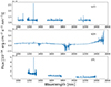 |
Fig. B.1. Flux-calibrated NIR spectra of Gaia18cjb. |
All Tables
Circumstellar extinction and accretion luminosity estimates for Gaia18cjb using empirical relations from Alcalá et al. (2017).
Optical photometry of Gaia18cjb we acquired and/or reduced. EFOSC r photometry was taken with Bessell R filter.
All Figures
|
Fig. 1. Hα line of Gaia18cjb from LT SPRAT spectrum. |
| In the text | |
|
Fig. 2. Visible (top) and IR (bottom) light curves of Gaia18cjb. The red circle highlights the Gaia Alert trigger. The error bars smaller than the symbol size are not presented. Grey dashed lines correspond to the epochs for which we collected NIR spectroscopy. |
| In the text | |
|
Fig. 3. Color-magnitude diagrams of Gaia18cjb based on data from Pan-STARRS data (yellow filled circles), ZTF, Konkoly, Mt Suhors, and WISE data before LUCI epoch (orange filled circles), and after LUCI epoch (blue filled circles). The arrows show the reddening vector, assuming extinction law from Cardelli et al. (1989) with RV = 3.1 (black arrow) and RV = 5.5 (red arrow), respectively. |
| In the text | |
|
Fig. 4. NIR color-color diagram of Gaia18cjb. Purple and red circles are pre-outburst data from 2MASS and UKIDSS observations in 2000 and 2010, respectively, while the brown and pink dots correspond to SOFI and GTC photometry in the burst phase (2021 and 2022, respectively). The blue dashed line and light blue region represent the CTTS locus and its uncertainty (Meyer et al. 1997), and the tiny blue dotted line its extension toward larger color indices. The orange solid and green dotted-dashed lines correspond to the colors of ZAMS and GB stars, respectively. The black arrow shows the reddening vector for a source with 1 mag of extinction (Cardelli et al. 1989, RV = 3.1). |
| In the text | |
|
Fig. 5. Spectral energy distribution. Circles and stars are observations taken before and after 2020, respectively. |
| In the text | |
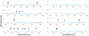 |
Fig. 6. Normalized LBT zJHK normalized spectrum. Emission lines reported in Table 3 are labeled. |
| In the text | |
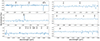 |
Fig. 7. Normalized SOFI spectrum. Emission lines reported in Table 3 are labeled. |
| In the text | |
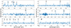 |
Fig. 8. Normalized GTC JHK spectrum. Emission lines reported in Table 3 are labeled. |
| In the text | |
|
Fig. 9. Extinction estimates of Gaia18cjb computed from the empirical relations between the accretion luminosity and Brγ and Paβ lines. Different colors represent AV estimates at different distances as described in the legend. |
| In the text | |
|
Fig. 10. Background of the figure is the Planck 857 GHz map, 10 degrees in size, centred on Gaia18cjb, the red star symbol in the plot. Blue and orange dots are sources with Hα-excess from Fratta et al. (2021) whose distances are 0.95 pc < d < 1.05 pc. The orange dots are sources whose proper motions are within 3 mas yr−1 from Gaia18cjb proper motions (see Fig. 11). The regions closes to Gaia18cjb are highlighted. |
| In the text | |
|
Fig. 11. Analysis on the young stellar nature of Gaia18cjb. Left: color-absolute magnitude diagram not corrected for the extinction. The red star symbol corresponds to Gaia18cjb. The black solid and dashed lines show the ZAMS and the 1 Myr isochrone, respectively (Dell’Omodarme & Valle 2013). Dots are sources which show Hα-excess from Fratta et al. (2021) catalog whose distance is 0.95 kpc < d < 1.05 kpc. Orange dots are sources with proper motions consistent within 3σ the propoer motion of Gaia18cjb (see right panel). The error bars smaller than the symbol size are not presented. The purple arrow represents an extinction vector of 1 mag. However, the AV vector depends on the color index and on the position in the diagram; see Prisinzano et al. (2022). Right: proper motions diagram of the Hα-excess sample. Symbols are the same as in the left panel. |
| In the text | |
|
Fig. 12. Accretion parameters as a function of the stellar parameters. Top:Lacc − L⋆ diagram. The red and black star symbols correspond to Gaia18cjb and EX Lup, respectively. The blue dashed line represents the Lacc = L⋆ locus. The grey line is the best fit for the CTTSs of Lupus from Alcalá et al. (2017) and the grey region corresponds to the standard deviation of the t. Bottom: Ṁacc − M⋆ diagram. Star symbols are as in the top panel. The grey line is the best fit for the CTTSs of Lupus from Alcalá et al. (2017) and the grey region corresponds to the standard deviation of the t. The pink area corresponds to Ṁacc ranges for embedded Class I+flat spectrum YSOs from Fiorellino et al. (2023). |
| In the text | |
|
Fig. B.1. Flux-calibrated NIR spectra of Gaia18cjb. |
| In the text | |
Current usage metrics show cumulative count of Article Views (full-text article views including HTML views, PDF and ePub downloads, according to the available data) and Abstracts Views on Vision4Press platform.
Data correspond to usage on the plateform after 2015. The current usage metrics is available 48-96 hours after online publication and is updated daily on week days.
Initial download of the metrics may take a while.