| Issue |
A&A
Volume 695, March 2025
|
|
|---|---|---|
| Article Number | A130 | |
| Number of page(s) | 19 | |
| Section | Stellar structure and evolution | |
| DOI | https://doi.org/10.1051/0004-6361/202451061 | |
| Published online | 12 March 2025 | |
Gaia20bdk – New FU Ori-type star in the Sh 2-301 star-forming region
1
Konkoly Observatory, HUN-REN Research Centre for Astronomy and Earth Sciences, MTA Centre of Excellence, Konkoly-Thege Miklós út 15-17, 1121 Budapest, Hungary
2
Mt. Suhora Astronomical Observatory, University of the National Education Commission, ul. Podchorążych 2, 30-084 Kraków, Poland
3
Institute of Physics and Astronomy, ELTE Eötvös Loránd University, Pázmány Péter sétány 1/A, H-1117 Budapest, Hungary
4
Max-Planck-Institut für Astronomie, Königstuhl 17, D-69117 Heidelberg, Germany
5
Department of Astrophysics, Türkenschanzstraße 17, 1180 Vienna, Austria
6
Institute of Astronomy, Faculty of Physics, Astronomy and Informatics, Nicolaus Copernicus University in Toruń, ul. Grudziądzka 5, PL-87-100 Toruń, Poland
7
Astronomical Observatory, University of Warsaw, Al. Ujazdowskie 4, 00-478 Warszawa, Poland
8
South African Astronomical Observatory, PO Box 9 Observatory, 7935 Cape Town, South Africa
9
Department of Physics, University of Johannesburg, PO Box 524 Auckland Park 2006, South Africa
10
Department of Physics, University of the Free State, PO Box 339 Bloemfontein 9300, South Africa
11
Department of Astronomy, University of Cape Town, Private Bag X3, Rondebosch 7701, South Africa
12
INAF-Osservatorio Astronomico di Roma, via di Frascati 33, 00040 Monte Porzio Catone, Italy
13
Instituto de Astrofísica de Canarias, IAC, Vía Láctea s/n, 38205 La Laguna (S.C.Tenerife), Spain
14
Departamento de Astrofísica, Universidad de La Laguna, 38206 La Laguna (S.C.Tenerife), Spain
15
Institut de Recherche en Astrophysique et Planétologie, Université de Toulouse, UT3-PS, OMP, CNRS, 9 av. du Colonel-Roche, 31028 Toulouse Cedex 4, France
16
Scottish Universities Physics Alliance (SUPA), School of Physics and Astronomy, University of St Andrews, North Haugh, St Andrews KY16 9SS, UK
17
Max-Planck-Institut für Radioastronomie, Auf dem Hügel 69, 53121 Bonn, Germany
18
Centre for Astrophysics, University of Hertfordshire, College Lane, Hatfield AL10 9AB, UK
19
Astronomical Observatory, Jagiellonian University, ul. Orla 171, PL-30-244 Kraków, Poland
⋆ Corresponding author; This email address is being protected from spambots. You need JavaScript enabled to view it.
Received:
11
June
2024
Accepted:
16
December
2024
Abstract
Context. We analyse multi-colour photometric and spectroscopic observations of the young stellar object (YSO) Gaia20bdk.
Aims. We aim to investigate the exact nature of the eruptive phenomenon that the star has been undergoing since 2018.
Methods. We used public-domain archival photometry to characterise the quiescent phase and to establish the major physical parameters of the progenitor. We used our own optical and infrared (IR) photometry and spectroscopy, along with data from the public domain, to study the outburst.
Results. Gaia20bdk is a member of the Sharpless 2-301 star-forming region, at a distance of 3.3 kpc. The progenitor is a rather massive 2.7 ± 0.5 M⊙, G7-type Class I young star, with an effective temperature of 5300−300+500 K and bolometric luminosity of 11 ± 2 L⊙. The optical and IR photometric and spectroscopic data obtained during the outburst reveal a variety of signatures commonly found in classical FU Ori-type stars (FUors). Our disc modelling gives a bolometric luminosity of 100 − 200 L⊙ and mass accretion rate of 1 − 2 × 10⁻⁵ M⊙ yr−1, also confirming the object’s FUor classification. Further monitoring is necessary to track the light changes, accretion rate, and spectral variations, as well as to understand the mechanisms behind the disc flickering.
Key words: accretion, accretion disks / stars: formation
© The Authors 2025
 Open Access article, published by EDP Sciences, under the terms of the Creative Commons Attribution License (https://creativecommons.org/licenses/by/4.0), which permits unrestricted use, distribution, and reproduction in any medium, provided the original work is properly cited.
This article is published in open access under the Subscribe to Open model. This email address is being protected from spambots. You need JavaScript enabled to view it. to support open access publication.
1. Introduction
FU Ori-type stars (FUors) were recognized by Herbig (1977) as classical T Tauri-type stars (CTTS) undergoing enhanced disc-matter accretion onto the forming star over a few decades or longer (see also Hartmann & Kenyon 1996). According to Fischer et al. (2023), in terms of the accumulated mass and luminosity rise, FUors represent the most spectacular end of the continuum of eruptive accretion in young stars. It is followed by EX Lupi-type stars (EXors), showing less dramatic eruptive events lasting a few months to a year, but re-appearing on a timescale of a few years (Herbig 1989), as well as intermediate cases (Audard et al. 2014) of eruptive stars showing properties of both FUors and EXors in various proportions; e.g. V1647 Ori (Andrews et al. 2004; Acosta-Pulido et al. 2007; Muzerolle et al. 2005), 2MASS 22352345+7517076 (Kun et al. 2019), V899 Mon (Ninan et al. 2015; Park et al. 2021), Gaia19ajj (Hillenbrand et al. 2019b), Gaia19bey (Hodapp et al. 2020), Gaia18cjb (Fiorellino et al. 2024), ASASSN-13db (Holoien et al. 2014; Sicilia-Aguilar et al. 2017), ASASSN-15qi (Herczeg et al. 2016), and a few dozens other objects discovered by Guo et al. (2024a).
According to Contreras Peña et al. (2019, 2024), Guo et al. (2021), and Fiorellino et al. (2023), eruptive events are much more common for Class I than Class II young stellar objects (YSOs) and all these stars are expected to undergo at least a dozen eruptive accretion events (Contreras Peña et al. 2019, 2024). These events have a major impact on the inner disc temperature, causing the expansion of the snow line of various volatiles (Cieza et al. 2016). Therefore, multi-wavelength studies of young eruptive stars (especially FUor events, lasting for several decades and centuries and thus having a major impact on the protoplanetary disc properties ) are crucial for understanding their chemical evolution and eventually also the composition and morphology of planetary systems, including our Solar System (Ábrahám et al. 2009, 2019; Hubbard 2017a,b; Molyarova et al. 2018; Wiebe et al. 2019; Kóspál et al. 2020, 2023).
The recently most recognised list of 26 FUors compiled by Audard et al. (2014) has been expanding constantly thanks to the ground- and the space-based sky surveys. Since 2014, the Gaia spacecraft has been observing each part of the sky in broad-band filters several dozen times a year (Gaia Collaboration 2016). After a few years of continuous observations, Gaia became an effective tool for catching long-term brightness changes in various astronomical objects down to 21 mag. The community is regularly notified about significant brightness variations via the Gaia Photometric Science Alert system (Hodgkin et al. 2021). Gaia17bpi (Hillenbrand et al. 2018) and Gaia18dvy (Szegedi-Elek et al. 2020) are the first two FUors discovered by Gaia. The spacecraft also played a significant role in recognizing ESO-Hα 148 (Gaia21elv) as a bona fide FUor (Nagy et al. 2023); we note that in contrast, to the previous stars, the alert was triggered due to a brightness decrease. Gaia was instrumental in the discovery of Gaia21bty, tentatively identified as a FUor by Siwak et al. (2023). Other FUors (or at least FUor candidates; among them Class 0 objects), were recently discovered from the ground and space-based infrared (IR) telescopes, such as PTF14jg (Hillenbrand et al. 2019a), PGIR 20dci (Hillenbrand et al. 2021), IRAS 16316-1540 (Yoon et al. 2021), WTP 10aaauow (Tran et al. 2024), SST-gbs J21470601+4739394 (Ashraf et al. 2024), VVVv721 (Contreras Peña et al. 2017; Guo et al. 2020), SPICY 99341 & SPICY 100587 (Contreras Peña et al. 2023), and L222-78 (Guo et al. 2024b), while in the accompanying paper, Guo et al. (2024a) present 15+ confirmed FUors. Finally, RNO 54 was recently recognized as a FUor by Magakian et al. (2023) and Hillenbrand et al. (2023).
The object of interest here, Gaia20bdk (αJ2000 = 7h10m14 92, δJ2000 = −18°27′01
 04), was identified by the Gaia Photometric Science Alert system on 2020 March 2 as a 1.2 mag brightening of a red star 2MASS 07101491–1827010 or Gaia DR3 2934263554310209536 (Gaia Collaboration 2023). The star is located in the outskirts of an optically bright nebula in Canis Major, only about 4 degrees from the Galactic mid-plane. The progenitor of Gaia20bdk was initially classified as Class I/II YSO candidate by Marton et al. (2016), and Class II by Pandey et al. (2022). The authors listed the star among a cluster of 37 identified YSOs, north-east of H II region Sharpless 2-301 (shortly Sh 2-301). During the modelling of these 37 YSO’s spectral energy distributions (SEDs), they determined typical extinction at AV = 5.8 mag and age 2.5 ± 1.6 Myr. The mass of our target was determined at 2.67 ± 1.5 M⊙. These authors also determined the distance to the cluster at 3.54 ± 0.54 kpc. This distance is in agreement with another determination 4.3 ± 0.6 kpc to the nearby bubble [HKS2019] E93 (Hanaoka et al. 2019; Hou & Han 2014). This is important as the Gaia DR3 catalogue does not offer a well determined parallax specifically for our target; the photogeometric distance obtained by Bailer-Jones et al. (2021) is
  pc.
pc.
We present and analyse new and archival data for Gaia20bdk and draw conclusions about its current nature. In Sect. 2, we describe the reduction of the archival photometry, and our new spectroscopic and photometric data obtained during the outburst until early 2024. The results obtained from the analysis are presented and immediately discussed in Sect. 3 and summarised in Sect. 4.
2. Observations
2.1. Pre-outburst photometry
In order to study the star during the quiescent phase, we collected archival public-domain visual and IR photometry. The earliest multi-epoch 2010–2014 optical data were obtained by the Panoramic Survey Telescope & Rapid Response System (PanSTaRRS) survey in the grizy-bands (Chambers et al. 2016; Magnier et al. 2020; Waters et al. 2020). We performed our own photometry of Gaia20bdk, using the aperture of 11 pixels ( ) and computed the sky within 13–27 pixels annulus. Then, to calibrate the results to standard magnitudes, we used the magnitude zero points provided in the headers for each image and filter. We compared our results to APASS9 gri magnitudes of stars in the same field determined by Henden et al. (2015, 2016), finding that their measurements are reproduced with our method within 0.05 mag, which is sufficient for our purposes. We show our results in Table A.1 in Appendix A and plot in Figure 1.
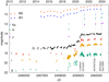 |
Fig. 1. Combined griJHKS light curves of Gaia20bdk obtained by several ground-based surveys and telescopes, and G, W1, and W2 light curves obtained by Gaia and (NEO)WISE space telescopes, as described in Sects. 2.1 and 2.2. The first JHKS data points from 1999 Feb 1 obtained by 2MASS were shifted forward by exactly 11 years, so they appear on this plot on 2010 Feb 1. |
Between 2014 December – 2021 September, observations in the griz-filters were collected by the SkyMapper wide-field survey by a 1.35-m telescope located at Siding Spring Observatory, Australia (Onken et al. 2019). In this paper we use the photometric data computed by the dedicated pipeline and available from the fourth data release (Onken et al. 2024). In nearly the same time, observations were made on two close epochs – 2017 February 4 and March 19 – at the European Southern Observatory (ESO), from the Cerro Paranal peak hosting the Very Large Telescope (VLT) and supporting telescopes. The data were obtained by means of the 2.6-m ESO VLT Survey Telescope (VST) equipped with the OMEGACAM and ugriHα filters, as part of VST Photometric Hα Survey of the Southern Galactic Plane and Bulge (VPHAS+; Drew et al. 2014). We performed photometry on the calibrated fits images downloaded from the public ESO archive using DAOPHOT II procedures (Stetson 1987) distributed within the astro-idl library. To ensure optimal extraction and to comply with our future observations (see in Sect. 2.2), the aperture of 20.95 pixel ( ) was used for the target and four comparison stars. The inner and outer sky annuli were specifically adjusted for each star between 25–50 pixels to enable accurate sky level calculation. We took the gri magnitudes of the four comparison stars from the APASS9 catalogue. As no colour trends were found, we simply averaged the results obtained from all comparison stars and computed standard deviation as the uncertainty measure (Table A.1, Fig. 1). The target was not detected in the u-filter; therefore, it was assumed to be fainter than 21.86 mag, as inferred from the magnitude zero point provided in the image header.
Starting in 2014, the Gaia spacecraft has been monitoring the sky more regularly. In Figure 1 we show the public domain light curve obtained in the G-band until November, 2023, thereby covering the rising branch and the outburst plateau.
The first pre-outburst near-infrared (NIR) data were obtained in JHKS filters by the 2MASS survey on 1999 Feb 1 (Skrutskie et al. 2006), while the second were taken on 2018 December 25-26, during the initial brightness rise (Pandey et al. 2022). On 2010 April 7, the IR data were collected during the fully cryogenic phase of the Wide-field Infrared Survey Explorer (WISE; Wright et al. 2010) in the W1, W2, W3, and W4 bands, centered at 3.4, 4.6, 12, and 22 μm, respectively. Then, in the post-cryogenic phase data were collected in W1 and W2-bands on 2010 October 15. From 2014 October, the NEOWISE mission continued to operate in W1 and W2-bands (Mainzer et al. 2011), providing long-term IR light curves covering the quiescent phase and the outburst. Usually, over a dozen individual measurements per filter were obtained during each of two (typically 2 days long) pointings towards our target. We downloaded individual catalogue measurements, removed obvious outliers, and computed the averages along with their standard deviations per each epoch (Fig. 1). Prior to this, to make sure that the measurements are unaffected by companions or nebulosity, we examined the individual images. We note that a saturation correction was not necessary.
2.2. Outburst photometry
We obtained our first observations of Gaia20bdk in BVRI Bessell filters on three nights from December 2020 to January 2021 at the South African Astronomical Observatory (SAAO). We used the modern 1-m Lesedi telescope, equipped with a Sutherland High Speed Optical Camera (SHOC), providing  field of view. To match typical seeing conditions, we chose a 2 × 2 binning resulting in 0
 666 pixel scale.
We continued optical monitoring at the Piszkéstető Mountain Station of Konkoly Observatory (Hungary) and at the Mount Suhora Observatory (MSO) of the University of the National Education Commission (Poland). In the first observatory we used the 80 cm Ritchey-Chretien (RC80) telescope equipped with an FLI PL230 charged-coupled device (CCD) camera, giving a 0 55 pixel scale and
  field of view, and Johnson BV and Sloan r′i′ filters; while in the second we used the 60 cm Carl-Zeiss telescope equipped with Apogee Aspen-47 CG47-MB CCD camera operating in the primary 2.4 meter focus, which results in the 1
 166 pixel scale and
  field of view. A modern set of BVRI interference filters manufactured by Custom Scientific was used.
Observations were also obtained at the ESO-LaSilla observatory on 2021 May 10. We used the 3.58-m New Technology Telescope (NTT) equipped with ESO Faint Object Spectrograph and Camera version 2 (EFOSC2) and BVR filters (Prog. ID 105.203T.002, PI: Giannini). With the 2 × 2 binning, the angular resolution is 0 24 per pixel.
The original frames were corrected for bias, dark, and flat field in a standard way in IRAF, while the RC80 data in IDL. For the MSO data, the correction for bias was accomplished using the same exposure used for dark, as well as for the science frames. For the photometric reduction, we used custom IDL scripts, utilising the astro-idl procedures from the DAOPHOT II package. The aperture photometry was always made in the same aperture size  , which translates to 4 pixels in MSO, 8.12 in RC80, 18.59 in EFOSC2, 6.66 in SHOC, and 20.95 at VST for pre-outburst photometry. The photometric calibration was done based on stable (to 0.02 mag) comparison stars, whose magnitudes were taken from the APASS9 catalogue. As this catalogue provides Bessell BV and Sloan g′r′i′ magnitudes, in the case of RI-filters, the magnitudes were inferred from interpolation of their SEDs for the effective wavelengths of those filters. The SEDs of these stars were constructed with the help of the 2MASS catalogue (Cutri et al. 2003). In the case of MSO and RC80 observations, performed usually between an airmass of 3–2.6, the correction for effects introduced by differential and colour extinction between each comparison star and the target were included. The mean first- and second-order extinction coefficients determined for MSO were used for both observatories. The MSO data were also transformed to the standard BVRI Johnson-Cousins system using colour transformation equations. These corrections considerably decreased the scatter between individual measurements and comparison stars, especially in the B-filter. In all observatories, 3–6 frames per filter per night were typically obtained. After the removal of obvious outliers (caused by satellite trails, guiding errors, cosmic rays) the results were averaged and the standard deviation was computed to estimate the uncertainty (Table A.2).
Multi-colour coverage of the outburst is also provided by the Zwicky Transient Facility (ZTF, Bellm et al. 2019). ZTF monitoring is conducted by means of the 48-inch Samuel Oschin Schmidt Telescope at the Palomar Observatory, equipped with a custom-built mosaic CCD camera and Sloan filters. Regular monitoring of our target with a 2 day cadence in gr-filters started on 2018 September 17, just 1-2 months before the star showed the first signs of the major brightness rise. We downloaded the data provided by the dedicated pipeline (Masci et al. 2019) from data release no. 20 (Fig. 1).
We also use the photometry obtained in the broad-band c (cyan) and o (orange) filters of the Asteroid Terrestrial-impact Last Alert System (ATLAS, Tonry et al. 2018; Smith et al. 2020; Heinze et al. 2018). The photometry was downloaded from the ATLAS Forced Photometry web service (Shingles et al. 2021). Although the data quality is low during the pre-outburst and the rising branch, it increases in the plateau. In combination with the 1 day sampling interrupted only by the seasonal breaks, this makes this dataset most suitable for studying the small-scale light variability during the plateau.
Our first NIR observations were obtained on 2021 May 9 by means of NTT equipped with the IR spectrograph and imaging camera, Son of ISAAC (SOFI, Moorwood et al. 1998). We constructed the ‘sky’ frame by taking the median of the five dither positions after scaling them to the same level, as computed by mode statistic. Then, as the resulting image was very uniform, we only subtracted the ‘sky’ frame from individual images and performed photometry on individual images in 4.88 pixel ( ) aperture and the sky ring in the range 15–30 pixels. For this purpose, we chose seventeen stable comparison stars from the 2MASS catalogue. The results obtained from individual images (after removal of obvious outliers) were averaged and the standard deviation was computed to estimate the uncertainty (Table A.2, Fig. 1).
One year-and-a-half later, on 2023 Jan 7, we performed observations in the JHKs filters of the NOTCam, installed on the 2.56 m Nordic Optical Telescope (NOT), located at the Roque de los Muchachos Observatory (La Palma, Canary Islands, Spain, Program ID: 66-103; PI: Nagy). For each filter, we used a five-point dither pattern with offsets of five pixels only. This small value and close vicinity of our target to the middle of the FoV, with an intersecting bad column and line separating four chip quadrants, caused severe difficulties in obtaining proper photometry. Given we were unable to compute a ‘sky’ frame as for NTT/SOFI, we used the dark frames obtained on the same night with the same exposure times as our science frames, as well as the sky flats. The flatfield was constructed as a mean of a series of images, each obtained by subtracting a ‘fainter’ from a ‘brighter’ image. The resulting science images (after dark subtraction and division by flat frames) show horizontal nonlinear gradients of the background, strongest at the target position. To remove these gradients, we applied an empirical correction, by computing and subtracting the median value of each line. Then, we also removed the bad intersecting column and line by taking the average of the two neighbouring columns and lines. These operations resulted in a uniform background in the entire FoV, including the close vicinity of the target. Images where the target’s point-spread function (PSF) was most seriously affected by the bad column and/or line, have been discarded from the scientific analysis. In other cases, we further limited potential distortion of target’s PSFs by using fairly small 6 pixel aperture ( ). The sky was computed in the ring of 11–22 for the target and 15–30 pixels for comparison stars (the same used for NTT/SOFI). We also obtained photometry from the J-band acquisition image, taken on the same night during the pointing setup for spectroscopic observations, where the target was placed in the CCD region that was unaffected by the bad columns. We obtained the same magnitude (well within the errorbars), which proves that our results (Table A.2, Fig. 1) should not be impaired by the procedures detailed above.
On 2023 December 3 and 4, followed by 2024 February 22, we performed photometry on mosaics obtained in JHK filters, each composed from a five-point dither, taken by the guide camera of SpeX. This is a medium-resolution 0.7–5.3 μm spectrograph, mounted on the 3.2-m NASA InfraRed Telescope Facility (IRTF) on Mauna Kea. The photometric calibration was done using the 2MASS magnitudes of a few faint stars visible in the small,  field of view (Table A.2, Fig. 1).
2.3. Low-resolution optical spectrum
On 2020 December 21/22 we observed Gaia20bdk by means of the SPectrograph for the Rapid Acquisition of Transients (SPRAT, Piascik et al. 2014), mounted on the Liverpool Telescope (LT; Steele et al. 2004), under ProgID: XOL20B01 (PI: Pawel Zielinski). SPRAT provides low spectral resolution (R = 350) in the range of 4020 − 7994 Å. The spectrum was reduced and calibrated to absolute flux units by a dedicated pipeline. The flux appears to be underestimated by 15–20%, as obtained by comparison with the nearly-simultaneous ZTF and SAAO griBVRI photometry. The low resolution of the spectrum makes it impossible to perform more detailed analyses; however, it clearly shows the Hα line in emission, while the Na Iλλ5890 and 5896, K Iλ7699, and O Iλ7774 triplet are seen in absorption (Fig. 2a).
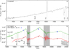 |
Fig. 2. Low-resolution LT/SPRAT spectrum (panel a), and the NTT/SOFI (2021 May 9) and the IRTF/SpeX (2023 December 3) low- and medium-resolution flux-calibrated spectra of Gaia20bdk (panel b). The grey-shaded areas in this panel demarcate regions strongly affected by telluric lines. The IRTF spectrum and photometry were shifted up by 3 × 10⁻¹⁵ erg cm−1 s−1 Å−1 for clarity. Only the major spectral lines and bands characteristic of FUors are indicated. Telluric absorption bands were not removed from the visual spectrum. |
2.4. High-resolution optical spectrum
On 2023 December 7 we used the High Resolution Spectrograph (HRS) mounted on the South African Large Telescope (SALT) under program 2021-2-LSP-001 (PI: Buckley). HRS is dual-beam, white-pupil, fibre-fed, échelle spectrograph, employing volume phase holographic (VPH) gratings as cross dispersers. Due to the low brightness of our target, we used the ‘low resolution mode’ (R ≈ 14 000, Crause et al. 2014). The spectrum was extracted, wavelength-calibrated, and corrected for the heliocentric-velocity by means of the dedicated pipeline (Kniazev et al. 2016, 2017). Despite using the longest possible exposure time for this declination (2400 s), the flux in the blue arm of the spectrum is almost zero. The flux increases only around 6000 Å, reaching signal-to-noise ratio (S/N) of 2-3 at the continuum, so that the Hα line clearly shows the P-Cygni profile, typical for FUors. The Li Iλ6707 line is undefined, but the spectra smoothed by means of Gaussian function of 5-10 pixel width show depression at the expected wavelength. Except for the K Iλ7699 line, the spectra are too noisy to show any well-defined absorption lines that could be used for radial velocity determination and analysis of the disc’s rotational profile. Another drawback is that the sky-fibre was most likely placed in the region with slightly brighter nebulae. Also, the wavelength calibration made by the pipeline resulted in shifts between the object- and the sky- fibres within each échelle order. Thus, in addition to the above problem, after the sky subtraction we observe strong artificial absorption lines. We identified those nebulae-related lines and distinguished them from terrestrial sky-lines by a manual scaling of the sky-spectrum intensity and subtracting it from the target spectrum. At the same time, the discrepancies in wavelength calibrations were to some degree averted for individual targets lines by manual shift of the sky spectrum in wavelength to match the position of sky lines observed in the target’s spectrum. It was only then that the subtraction of the corrected sky spectrum from target spectrum resulted in satisfactory results.
2.5. Near-infrared spectroscopy
On 2021 May 9, we obtained our first NIR spectrum by means of SOFI on NTT (Prog. ID 105.203T.002, PI: Giannini). We used the low-resolution blue and red grisms with GBF and GRF order sorting filters through the 0.6 arcsec wide slit, covering 0.95 − 1.64 and 1.53 − 2.52 μm with R = 930 and 980, respectively. We reduced the spectra in IRAF: first the thermal noise and the sky level were approximately removed by subtraction of images obtained in consecutive A and B nod positions. We skipped the flat-fielding as this operation slightly increased the background scatter of the otherwise fairly smooth differential images (i.e. consecutive A-B pairs), as well as the overall scatter of the extracted spectrum. Due to the field curvature, further steps were performed using the tasks under the longslit package: the xenon lamp spectra and respective line lists provided for SOFI users were used for the wavelength calibration, performed with the (re)identify, fitcoords, and transform tasks, to transform the original (x, y) image coordinates into the (x, λ). The apall task, with variance weight extraction method and with sky-residuals removal by median, was used for spectrum extraction. Finally we removed atmospheric lines using the telluric task, where we interactively scaled the normalised spectrum of the telluric standard star HD143520, obtained on the same night, but at different airmass and hour angle; however, this did not affect the cleaning process. Finally, we combined the individual telluric-corrected images to form average ‘blue’ (0.95 − 1.64 μm) and ‘red’ (1.53 − 2.52 μm) spectra. We then approximately flux-calibrated the spectra to the simultaneously obtained JHKS photometry. The response function was estimated by means of the Planck spectrum closely aligned to the JHKS points, with the help of nearly-simultaneous rRiIW1W2 photometric points (Fig. 2b). Only the blue edge of the response function was not perfectly estimated, so that the spectrum level is slightly underestimated below 10 000 Å.
On 2023 Jan 7, we obtained the second low-resolution NIR spectrum by means of NOTCam (Program ID: 66-103; PI: Nagy). We reduced the spectra in the same way as SOFI spectra. Argon arc lamp was used for J-band wavelength calibration and xenon for the H and K. We also decided to skip the flat-fielding operation as it only increased the noise in the extracted spectrum and/or disturbed its otherwise smooth shape. A telluric correction was achieved using HD56405 spectrum, observed at very similar airmass and hour angle as the target. Despite having the simultaneous JHKS photometry, we decided to skip the flux-calibration of the spectrum due to a ‘rectangular’ response function of all gratings, making the proper shape of the spectrum hard to recover.
The third and the best set of NIR spectra was obtained on 2023 December 2 and 3 (Program ID: 2023B037; PI: Kóspál) by means of the IRTF equipped with SpeX (Rayner et al. 2003). SpeX is a medium-resolution IR spectrograph, which we used in the Short XD (SXD) mode, providing spectra in the range 0.7 − 2.55 μm. We used the 0.8 × 15 arcsec slit, providing a spectral resolution of R = 800. The integration time of the single spectrum was 180 s. We collected 11 spectra on the first night and 12 spectra on the second. Following the spectrum extraction by the SPEXTOOL software (Vacca et al. 2003; Cushing et al. 2004), a telluric correction was performed using the A0V stars HD20995 on the first night, and HD65102 on the second. Due to a rapidly increasing cloudiness during the end of the first night, the telluric standard was observed in the close vicinity of the target only on the second night. We calibrated these spectra to absolute flux by matching to the JHKS photometry obtained on the second night (Fig 2b).
3. Data analysis
3.1. Further insights into the distance
Rather than adopting the literature value for the distance to the target (Sect. 1), we sought to refine it using data from Gaia DR3. A recent study for open clusters shows that Gaia20bdk shares common proper motions with the members of the open cluster [DBS2003] 3 (Dutra et al. 2003), comprising part of the NE part of the Sh 2-301 star-forming region. This cluster can also be found in other catalogues (e.g. Kharchenko et al. 2013; Cantat-Gaudin et al. 2020; Pandey et al. 2022; Hunt & Reffert 2023). The mean distance obtained by Hunt & Reffert (2023) for [DBS2003] 3 is 3.3 kpc, comparable to the distance others found. Analysing the distance distribution of the member stars, we adapted the uncertainty of ±0.3 kpc. We use these values throughout this paper.
3.2. General description of the variability
Based on the Gaia light curve displayed in Fig. 1, the object had quiescent brightness of G = 18.95 ± 0.15 mag, and this situation lasted until mid-November, 2018. Since then, until about mid-November, 2019, Gaia measurements started to show little brightening to G = 18.44 ± 0.13 mag. This initially slow brightening process accelerated sometime in December, 20191, which ultimately led to the Gaia Alert issued on 2020 March 2. Gaia20bdk continued the fast brightening until mid-December, 2020, when it peaked at 16.02 mag. In the next few months it slightly dropped to ∼16.2 mag, but immediately started slow rise with superimposed wave-like variability (G = 16.11 ± 0.08 mag) – we call this stage as ‘plateau’ later in this paper. The total brightness rise from the mean quiescent level to ‘the first peak’ was ΔG = 2.93 mag. Due to the slow brightening trend in the plateau and the wave-like variability, ΔG reached 3 mag for a short time in 2023. We note that this two-stage brightening behaviour is very similar to what was found for HBC 722, as described by Kóspál et al. (2016) in their in Sect. 3.1.
The same evolution is observed in gri light curves, combined from the data collected by PanSTaRRS, SkyMap, VPHAS+, ZTF, and at the Piszkéstető Mountain Station (Fig. 1). The quiescent levels in these filters were g = 21.48 ± 0.12, r = 19.51 ± 0.20 and i = 18.16 ± 0.12 mag. After the initial (Nov, 2018 – Nov, 2019) slow brightening phase, the brightening rate increased and, in December, 2020, the light curves initially peaked for a few days at 17.76, 16.02 and ∼15.02 mag in gri-bands, respectively. Similarly to what is seen in the G-band, the brightness dropped slightly after ‘the first peak’, then rose and started to vary around g = 18.30 ± 0.17, r = 16.28 ± 0.11 and i = 15.24 ± 0.11 mag. The total brightness rise from the quiescent level to ‘the first peak’ was Δg = 3.86, Δr = 3.44, Δi ≈ 3.14 mag. Due to the brightening trend (slower in the g band, but faster in the ri bands), these values may be crossed in the near future.
Information extracted from the JHKS bands is less accurate due to worse sampling. Based on 2MASS and NTT/SOFI observations, we got ΔJ ≈ 2.57, ΔH ≈ 2.30 and ΔKS ≈ 2.08 mag. The brightness is also slowly rising during the plateau. This is even more evident in NEOWISE data, where after the quiescent stage (W1 = 10.51 ± 0.20 and W2 = 9.57 ± 0.21 mag), in 2017 and 2018, the brightness started to rise with almost constant rate until 2022. To estimate the amplitude at the same moment as for the optical bands (‘the first peak’), we interpolated between the points obtained just before and just after December, 2020. We got W1 ≈ 9.21 and W2 ≈ 8.53 mag, which gives ΔW1 ≈ 1.30 and ΔW2 ≈ 1.04 mag. In October 2022, and March 2023, the values were higher by 0.3 mag.
To extract more accurate information about the outburst timing in different bands, we fit the analytical logistic function in the form m = m0 − Δm/(1 + e−(t − t1/2)/τ)) to the sufficiently well sampled light curves in grGW1W2 filters (Hillenbrand et al. 2018; Kuhn et al. 2024; Guo et al. 2024b). In this function, m0 is the quiescent magnitude, known from the observations and listed above. The adjustable parameters are t1/2 (the midpoint of the rising branch), Δm (the outburst amplitude2), and τ (the characteristic timescale of the brightness growth). We show the results in Figure 3a. However, the combination of the short timescale secular variability superimposed on the major outburst – especially strong in the optical bands during the brightness rise in 2018-2020 (Fig. 3b) – and the nonuniform sampling caused a failure of the analytical method. There is especially no consensus in t1/2, that is, we did not observe any monotonic wavelength-dependency (as reported by the authors cited above). In our case, t1/2 changes from JD − 2458000 = 875, 885 and 965 d for grG and then returns to 840 and 900 for W1W2, respectively. We see some evidence of a trend in the characteristic brightness increasing over time, τ0, which gradually progressed from 103 ± 4, 105 ± 10, 125 ± 6 d in grG to 370 ± 55, and 445 ± 70 d in W1W2.
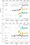 |
Fig. 3. Analytical fits of logistic function to the best sampled grGW1W2 light curves (panel a). Second panel shows the residuals after subtraction of respective logistic functions. |
At first glance, the visual analysis and trend seen in τ0 may suggests that the outburst could start first in the W1W2 bands; namely, around 2017/2018, which is one year earlier than noticed in the grG-filters. However, this is likely to be the result of some confusion, due to the significant (of about ±0.2 mag) quiescent variability in the W1W2 bands (Fig. 3b), as compared to the total brightness rise (ΔW1 ≈ 1.30 and ΔW2 ≈ 1.04 mag). We note that the local minimum visible in the end of 2017 (which on the first sight may look as the outburst start in the IR bands) is similar to that from the beginning of 2015, which suggests (quasi-)periodic event. Taking this fact into account we cannot exclude that the outburst could in fact start later in the W1W2 bands, possibly in the middle of 2018 (or even together with the optical bands). Therefore, we conclude that there is no clear evidence of an outside-in outburst propagation mechanism, as seen for Gaia17bpi and Gaia18dvy (Hillenbrand et al. 2018; Szegedi-Elek et al. 2020). Our data suggest, instead, that this outburst has been driven in a similar way to what is seen in HBC 722, that is, by a rapid increase in accretion caused by piled-up material from the inner disc leading to ‘the first peak’ (and perhaps the earlier variation best seen in the 2019 residuals), followed by a slower outward expansion of a hot component, as predicted by Bell et al. (1995). However, we do not have enough measurements to prove this (as noted in Sect. 3.8) analytically as accurately as reported in the work in Kóspál et al. (2016) and, most recently, Carvalho et al. (2024).
3.3. Small-scale variability
In addition to the major outburst, the sufficiently well sampled grioGW1W2 light curves show low-amplitude (typically 0.01–0.2 mag) light changes, some of them likely quasi-periodic oscillations (QPOs). In the pre-outburst stage they are visible as ∼2 yr variation in the W1W2-bands (Fig. 3a), then they improve a bit after the subtraction of the respective logistic functions (Fig. 3b)3. Until mid-2018 the variation remained invisible in (at the time best sampled optical) rG-bands. The 2 yr variation apparently continues during the plateau in the IR bands, but with a smaller amplitude, which is probably due to the increase in disc temperature. The variation also became visible in the optical bands, while our measurements of the G-band light curve have refined the period to 1.8 ± 0.2 yr. In the case of the g-band, the 1.8 yr QPO appears to be less securely defined, which is probably caused by a combination of the dominant inner disc high frequency variability and the lower photometric precision. The 1.8 yr QPO suggests 2 au location, assuming it is caused by Keplerian rotation of a disc inhomogeneity around 2.67 M⊙ star. However, during the outburst this variation is visible at shorter wavelengths as well, as the disc temperature increased and the previously colder disc annuli dominating at IR wavelengths during quiescence became more active in the optical ones. A few more years of multi-colour monitoring, supported by high-resolution spectroscopy, will shed more light on the physics behind the 1.8 yr QPO.
The above low-frequency variations are not the only ones visible in the residuals. According to Fig. 3b, the largest variations are noticed in 2019–2021 during the rising branch, when they reached 1 mag in the gr-bands. Amplitude of these oscillations gradually decreases towards longer wavelengths, but they are still visible by NEOWISE. One can notice likely positive correlation between variability in optical and IR bands. Similar conclusion can be drawn with regard to ‘the first peak’, which we conventionally treat as the beginning of the plateau. We speculate that ‘the first peak’ may have common driving mechanism with the preceding 1 mag variation from 2019.
Subsequently, the best-sampled o-band ATLAS data show various light changes occurring in the timescales of days, weeks, and months during the plateau (Fig. 4a). These light changes are also visible in the grG data, but in much less detail due to sparse sampling. Therefore, the Sloan-filter data were not taken into account in the frequency analysis; however, they are included in the discussion (Sect. 3.4) of the investigation of colour properties of the small-scale light variations during the plateau.
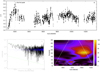 |
Fig. 4. ATLAS o-band light curve obtained during the plateau, with the slow brightening trend removed (panel a). The second panel shows Fourier spectrum (black line) in the log-log scale, calculated from the o-band data taken during the plateau and transformed to normalised flux unit. The flickering noise nature (af ∼ f−1/2) of these oscillations is indicated by the two parallel green dashed lines, while the amplitude errors are represented by blue dots. Third panel (c) shows respective WWZ spectrum. The major edge effects lie outside of the white dashed lines. The WWZ power is expressed in colours, as shown in the right label. |
To perform a frequency analysis of the o-band time series, in the first step, all outliers were manually removed. The long-term trend in brightness was removed by a second-order polynomial fit (Fig. 4a). Then the magnitudes were transformed to flux units, normalised to unity at the mean brightness level. The Lomb-Scargle diagram (Zechmeister & Kürster 2009) reveals a dozen of significant peaks (with the false alarm of probability of 10−10 : −36), especially at 68 and 207 days. Still, none of them represent a stable period or quasi-period. Instead, in accordance with visual inspection, they usually exhibited only two quickly disappearing oscillations. We also computed a Fourier spectrum, as described in Siwak et al. (2013). It shows the flicker-noise nature of the light changes, as the spectrum amplitude af scales with the frequency, f, as af ∼ f−1/2 (Press 1978). This relation is indicated by the two parallel green dashed lines in Fig. 4b. This feature of the Fourier spectrum is typical in a variety of accreting objects (Scaringi et al. 2015) and was studied for the first time in FU Ori by Kenyon et al. (2000). According to the authors, flickering is observed as a series of random brightness fluctuations with amplitudes of 0.01–1.0 mag that recur on dynamical timescales (a feature observed during Gaia20bdk’s plateau); therefore, they believed to be a dynamical variation of the energy output from the disc.
A wavelet analysis allows us to trace temporal changes and localise in time finite oscillatory packages. The goal of this analysis is to get deeper insights into the physical processes occurring at different disc annuli, which make up the entire flicker-noise spectrum (Siwak et al. 2013, 2018). Due to non-uniform coverage from the ground, instead of a wavelet analysis applied to a uniformly sampled space-base data, here we computed the weighted wavelet Z-transform (WWZ) proposed by Foster (1996). The major edge effects are indicated by the two white lines, which means that significant signals are contained only inside the trapezium region defined by these lines. We show only signals longer than 10 days, to avoid spurious results at the highest frequencies, most seriously affected by non-uniform sampling. We also decided to cut-off ‘the first peak’ and start the analysis from HJD = 2459263, as the strong variation caused by ‘the first peak’ strongly re-scaled the spectrum’s dynamical range, worsening the visibility of the more subtle features. Our examination of the WWZ spectrum (Fig. 4c) suggests that the 68 ± 10 d signal could represent the final stage of a drifting QPO, which starts as a 115 d signal. However the significance of this drifting feature before it reached 68 d is low due to poor data coverage in the beginning of the plateau. After that the WWZ spectrum became dominated by the 207 ± 25 d signal. Further monitoring should reveal whether it is just a single oscillatory event or whether it represents the beginning of a new QPO. The WWZ spectrum also reveals a handful of isolated low-significance events at 15–40 d periods; these may, in fact, be identified directly in the light curve after a more careful visual inspection. It is possible that some of them lasted for a few cycles, which would enable to classify them as ordinary QPOs, but this is impossible now due to unequal sampling from the ground. If they are indeed ordinary QPOs, they could stand as the equivalent of the 11 day family in FU Ori itself (Siwak et al. 2018), likely appearing at the sharp drop in the disc temperature (Zhu et al. 2020).
The one- and two-dimensional frequency analyses performed above did not firmly reveal time-coherent light variability patterns, as in FU Ori (Siwak et al. 2013, 2018), as well as possibly in V2493 Cyg (Green et al. 2013; Baek et al. 2015) and V646 Pup (Siwak et al. 2020). As for now, the available data suggest that Gaia20bdk shares common properties with FUors with larger AV values, such as V1057 Cyg (Szabó et al. 2021) and V1515 Cyg (Szabó et al. 2022), where TESS data revealed incoherent light changes of even stronger af ∼ f−1 stochastic (Brownian) nature, but evolving towards flicker noise (af ∼ f−1/2) in ground-based data; namely, at frequencies like those those investigated here. In the case of V1057 Cyg, Szabó et al. (2021) speculated that apparently the stochastic ‘Brownian motion’ of hypothetical clumpy condensations in the disc wind destroyed the coherence of the incoming light; namely, information that the light from the innermost disc is carrying. Longer, preferably space-based monitoring would resolve this ambiguity. We checked that angular resolution provided by TESS is unfortunately too low to study these issues for our target.
3.4. Colour-magnitude diagrams
Colour-magnitude diagrams (CMDs) composed of gri-band data obtained in various observatories show that the transition from the quiescence to the outburst stage did not occur due to the reduction in the extinction (Fig. 5a and b). The extinction path, computed for Sloan filters by applying the Cardelli et al. (1989) law for total-to-selective extinction RV = 3.1 and AV = 3.2 mag, is indicated as the red semi-arrow. Due to the fact that observations in quiescence were never obtained simultaneously in all bands, we computed the colour indices by pairing data obtained ± 90 days apart. Thus, these data cannot be used for detailed colour variability studies in the quiescence, but just as an indicator of the mean value of the quiescent colour index. Later, during the rising and the plateau, we computed the colour indices by pairing points obtained during the same night.
 |
Fig. 5. CMDs in the optical and IR part of the spectrum. The (NEO)WISE data are colour-coded: blue represents the quiescence, yellow: the rising branch and red: the plateau. The bottom line shows two diagrams computed from the detrended ZTF and RC80 gri data taken during the plateau only. |
Near-IR CMDs in the JHKS filters, colour index versus time and CMDs based on NEOWISE W1W2 photometry are shown in Fig. 5c, d, e, and f, respectively. According to the CMDs composed of the ground-based JHKS data (Fig. 5c and d), the transition from the quiescent phase to the outburst cannot be explained by reduction in the extinction, which is similar as seen in Sloan bands. Even though the NEOWISE data obtained during the major brightness rise (marked by yellow) are distributed along the extinction path, the observed brightness and colour change is much higher than expected just via a ΔAV = 3.2 mag reduction. We note that although the brightness in the W1W2 bands was increasing until 2022/2023, the points obtained after ‘the first peak’ (2020/2021, marked by red) are showing different trend, similar to that seen in quiescence (marked by blue).
An analysis of the CMDs obtained during the plateau to understand the colour properties of the flickering (Sect. 3.3) is difficult due to the observing strategy adopted in the ZTF survey, providing the only source of nearly simultaneous multi-colour data. In that survey, data in distinct Sloan filters are usually obtained a few hours apart, so that the colour indices are of lower precision. The strategy was much more unfortunate in the case of ATLAS, where the data in co-bands were usually obtained on different nights (and therefore rejected from our colour analysis). We performed a least-squares fitting (weighted by xy errors) of a linear function to the trends observed in the CMDs composed of ZTF and Piszkéstető data obtained during the plateau. The best fit is indicated by the black line and the 1-sigma errors in the slope are indicated by the grey-dashed lines. There is a very weak signature, where the data points in the (g − r)−r CMD show the star being bluer when brighter (Fig. 5g). Slightly more significant is the distribution observed in the (r − i)−r diagram, showing that the star is redder when brighter (Fig. 5h). This result is similar to that obtained from fits to respective Johnson filters in FU Ori by Kenyon et al. (2000). The temperature of the flickering source obtained by the authors suggested the G0 I spectral type, which is the inner disc atmosphere. We decided not to investigate that issue in detail here, as the proper treatment of such CMDs requires more accurate, preferably space based light curves to determine associated QPOs, if exists (Siwak et al. 2018, 2020; Szabó et al. 2021, 2022). We plan to return to this topic in a few years, once long, uniformly sampled, accurate light curves in (preferably) several filters are available.
3.5. Determination of AV during the quiescent phase from the NIR colour-colour diagram
In Figure 6, we present the J − H vs. H − KS colour-colour diagram and the empirical position of unreddened CTTS established by Meyer et al. (1997). Works in the iterature and our own (see Sects. 1, 3.7) indicate our target does not reveal a very embedded Class I membership. The colour-colour diagram itself suggests that the progenitor of Gaia20bdk is a rather ordinary, but substantially reddened CTTS. Assuming RV = 3.1 for Cardelli et al. (1989) extinction law, we obtained AV = 5.9 ± 0.1 mag during the only epoch covered with NIR pre-outburst observations obtained by 2MASS. A slightly larger value is seen in the data of Pandey et al. (2022), but we skipped this determination, as those observations were obtained during the initial brightness rise of Gaia20bdk.
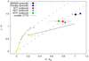 |
Fig. 6. J − H vs. H − KS colour-colour diagram prepared from pre-outburst (2MASS and Pandey et al. 2022) & outburst (SOFI, NOT, IRTF) data of Gaia20bdk. The squares represent zero age main sequence (ZAMS) stars, while the open circles show giant branch (GB) stars (Bessell & Brett 1988). The black line is the locus of unreddened CTTS (Meyer et al. 1997). The two parallel lines formed from pluses represent the reddening path; the step represents the reddening by additional 1 mag in AV. |
3.6. Determination of AV during the outburst phase from the NIR spectra
As the extinction towards FU Ori is low and relatively well determined (AV = 1.7 ± 0.1 mag; see in Zhu et al. 2007; Siwak et al. 2018; Green et al. 2019; Lykou et al. 2022), we used another approach to determine the interstellar extinction towards our target – during the outburst instead. This method relies on a considerable similarity of all bona fide FUor spectra in NIR, and follows the methodology of Connelley & Reipurth (2018) with respect to checking how much de-reddening ΔAV should be applied to our NIR flux calibrated spectra to match the calibrated spectrum of FU Ori (but scaled to match the flux level of the target). For the single NTT/SOFI GB- and GR-band flux-calibrated spectra, we obtained the best match for ΔAV = 4.0 ± 0.1 mag. In the case of the two IRTF/SpeX spectra, the best match was also found for ΔAV = 4.0 − 4.2 mag. This results in AV = 5.7 ± 0.2 mag and AV = 5.6 − 6.0 mag towards Gaia20bdk during the outburst, respectively. These values are consistent with AV = 5.9 ± 0.1 mag obtained in Sect. 3.5 during quiescence. This means that the increased disc wind caused by the outburst itself did not lead to the substantial drop in extinction, as sometimes observed in young eruptive stars like Gaia19ajj (Hillenbrand et al. 2019b).
3.7. Analysis of the quiescent SED. The progenitor
Based on WISE magnitudes and using equation 8 in Kuhn et al. (2021), we derived the spectral index, α, in the range of +0.3 to −0.6 for the pre-outburst SED (Fig. 7a). Assuming that the single W4 measurement is representative for the entire pre-outburst stage, this suggests either Class I or flat-spectrum membership for Gaia20bdk.
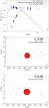 |
Fig. 7. Pre-outburst SED suggesting either flat spectrum or Class I membership (panel a). The same panel shows results of the dereddened quiescent data modelling. Position of the star in the H-R diagram based on modelling results (panels b&c); the one obtained with the assumption of the optimal temperature (5300 K) and distance (3.3 kpc) is indicated by the largest dot. The size of the dot fairly well represent the uncertainty in L* and R* caused by uncertainty in distance (3.0–3.6 kpc); Similar size should be applied to the two small dots to indicate uncertainties. |
In addition to the data described above, using the pre-outburst de-reddened data, we derived the physical parameters of the progenitor in order to supplement those presented by Pandey et al. (2022). For this purpose, we manually aligned a few dozens of Planck functions, computed for different effective temperatures Teff and stellar radii R⋆ (with 100 K and 0.5 R⊙ steps, respectively) to the lower part of the data, coming from the 4800–9200 Å region (i.e. to 2–5 points with lowest flux densities per wavelength bin). This choice was dictated by the lack of obvious dips in the pre-outburst stage, which suggests that most of the variability came from the ordinary low-state accretion typical for CTTS. Bearing in mind that blue wavelengths are more enhanced by accretion effects and that the disc radiation starts to dominate over the stellar one roughly from the J-band, we derived the best fits for  K (Fig. 7a). For a distance of d = 3.3 kpc, this results in a stellar radius
  R⊙. The ±0.3 kpc uncertainty in the distance introduces an extra ±0.5 R⊙ uncertainty to R⋆ in addition to the listed above (±1 R⊙ in total).
We integrated the Planck function over the entire wavelength range. Assuming that the solar bolometric luminosity is L⊙ = 3.85 × 10⁻³³ erg s−1, we derived a bolometric luminosity of the progenitor of L⋆ = 11.3 L⊙ for 5000 K and 5300 K (SpT G7), and 12.4 L⊙ for 5800 K. The more realistic uncertainty in L⋆ is related to uncertainty in distance and for the most reliable temperature (Teff = 5300 K), the values are seen to change from 8.7 L⊙ for 3 kpc, to 14.5 L⊙ for 3.6 kpc. Our results superimposed on the evolutionary tracks of Siess et al. (2000) confirm the mass 2.67 ± 1.50 M⊙ derived by Pandey et al. (2022) (Fig. 7b and c); however, our results strongly suggest that the real mass uncertainty is smaller, namely, about 0.5 M⊙. We also explored the grid of evolutionary tracks prepared for different ages by Siess et al. (2000) in mass, radius, effective temperature, and luminosity. Most of them indicate an age of 2–3 Myr for Gaia20bdk, but 0.5–4 Myr is also possible.
3.8. Analysis of the outburst SED. Determination of the mass accretion rate
The accretion disc model introduced by Kóspál et al. (2016) for HBC 722, and then applied to other FUors (Szabó et al. 2021, 2022; Nagy et al. 2023; Siwak et al. 2023) was used here to extract more information about the outburst physics. For this purpose, we first constructed three separate outburst SEDs from the data gathered in JHKS filters on 2021 May 9 (epoch 1), 2023 Jan 7 (epoch 2), and 2023 December 3 (epoch 3), along with the griBVRIW1W2-band data, usually interpolated from the closest data points. The errors of all data points were conservatively assumed to be 5%. As no information on system geometry was available, we set the disc inclination at i = 60 deg because cos i = 0.54. The radius of the inner disc was assumed to be equal to the stellar radius Rin = 4.0 ± 0.5 R⊙. The errors of the remaining parameters were derived using the models computed for the upper (4.5) and lower (3.5) values of Rin. For each epoch, we considered three values of the distance: 3.0, 3.3, and 3.6 kpc. The passive disc component (e.g. Liu et al. 2022; Carvalho et al. 2024) was roughly estimated and taken into account during the search for the outer disc radius, Rout, for each epoch.
For epoch 1, our best-fit model for the most likely distance (3.3 kpc) resulted in an outer disc radius of 0.3 au (0.4 au with passive disc emission component unaccounted), disc bolometric luminosity of Ld = 133 L⊙, MṀ = 4.0 × 10⁻⁵ M⊙2 yr−1 (where Ṁ is the mass accretion rate), and AV = 4.75 mag. The last parameter is 1.2 mag lower than the value determined in Sects. 3.6 and 3.5. We speculate that this may be due to the model imperfections and possibly by the fact that in all cases, our extinction estimates are based on photometric and spectroscopic data gathered in JHKS-bands.
The fit to epoch 2 data is less accurate (χ2 = 9.23). The best fit resulted in higher outer disc radii, about 0.8 au (1–1.1 au with passive disc emission component unaccounted) and slightly lower Ld and MṀ. We also encountered problems with the proper reproduction of AV, which resulted in 4.15 mag only.
We encountered the same dilemmas with model-returned AV = 4.70 mag when modelling the epoch 3 dataset. The model resulting in the most realistic parameters gave χ2 = 3.60. As for epoch 1, we obtained 0.4 au for the outer disc radius (0.5–0.6 au with passive disc emission component unaccounted). The disc luminosity is higher (165 L⊙) than in earlier epochs and the same is true for MṀ. We show the modelling results for d = 3.3 kpc in Figure 8.
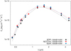 |
Fig. 8. Results from disc modelling of SOFI, NOTCam and SpeX data (i.e. Epoch 1, 2, and 3, respectively), as shown in Table 1. |
Taking d = 3.3 kpc and a stellar mass of 2.67 M⊙, we calculated a mass accretion rate of Ṁ = 1.50 × 10⁻⁵ M⊙ yr−1 during the first epoch, Ṁ = 1.24 × 10⁻⁵ M⊙ yr−1 during the second, and Ṁ = 1.78 × 10⁻⁵ M⊙ yr−1 during the third. Based on results listed in Table 1, slightly larger values of Ṁ can be derived for d = 3.6 kpc, while smaller ones would be seen for 3.0 kpc. The uncertainty in the stellar mass given by Pandey et al. (2022) affects the results more seriously (to ±60%), but even then, the mass accretion rate remains in the range typical for FUors. We do find, however, that the real uncertainty in mass is much smaller based on evolutionary tracks (Fig. 7b and c) and it does not exceed 0.5 M⊙, so that the Ṁ computed from individual models are accurate to about 20–30%.

The variations of the outer disc radius seen in the three epochs are probably not real. They appear to be a side effect of the non-negligible small-scale variability observed in all bands. We found that SEDs from epochs 1 and 3 were composed of measurements obtained close to the local light minima, whereas those of epoch 2 were obtained during the local light maximum. Future observations may let us determine the mechanism staying behind these small-scale light variations, and to determine Rout in an unambiguous way.
3.9. Spectral features and their variability
Our spectra of Gaia20bdk contain all features commonly found in spectra of classical FUors, as summarised by Connelley & Reipurth (2018). The most pronounced are the strong molecular Δν = 2 CO band heads absorptions (starting from 2.29 μm in the K-band) and the triangular shape of the entire H-band, caused by water vapour absorption typically observed in low-gravity young stars (Fig. 2b). The spectra also show the two major absorption lines in the J-band, He I and Paβ (although, on 2021 May 9, the second line was likely still in emission or equal to the continuum). Both 2021 and 2023 spectra show TiO and VO molecular absorption bands. The first dominate the red part of late-type stars spectra, while the second are typical of higher luminosity M7 stars, but absent in M-dwarfs. We mark these sharply starting bands by continuous black lines and arrows in Fig. 2b, similarly to the beginning of the water vapour absorption (H2O).
In addition to Paβ, the more detailed look into the J-band spectra reveals Paγ and Paδ (Fig. B.1a). These were likely to be in emission or undetected in 2021 May 9, but they are very well defined in spectra from 2023 December. Attempts to find Paα (1.875 μm) failed, even in the best SpeX spectrum due to strong contamination of this region by telluric lines.
We identified five lines from the Bracket series in the H-band (Fig. B.1b). They are typically weak in FUors; thus, they are most visible in the SpeX spectra, which have the best signal-to-noise ratio (S/N) among the spectra we obtained. Positions and names of six undetected or tentatively detected lines from the Bracket series are indicated for completeness, but these are marked with question mark. In the K-band SpeX spectra we also detected Brγ showing P-Cygni profile (Fig. B.1c), as typically observed in classical FUors by Connelley & Reipurth (2018).
In addition to the major CO bands visible in the K-band, in the H-band, we also identified three (out of six) lines belonging to the Δν = 3 band head. We mark their positions with solid black lines. The first two lines closely coincide with positions of other lines, but detailed look reveals stronger broadening (caused by lines merging/blending) and two separate bottoms (local minima) at the expected positions of each line. Other young eruptive stars also show this CO series, such as Gaia19ajj (Hillenbrand et al. 2019b), PGIR20dci (Hillenbrand et al. 2021), V960 Mon, and RNO 54 (Hillenbrand et al. 2023).
We also detected metals commonly found in other FUors by Connelley & Reipurth (2018). Many of these positive detections we owe to the SpeX spectra, which reveal Na I and Ca I in the K-band, Mg I in the H-band, and AlI, and Na I in the J-band. Following the authors cited here, we measured the equivalent widths (EWs) of Na I, Ca I and the first Δν = 2 CO band overtone (measured from 2.292 to 2.320 μm), obtaining EW(Na I+Ca I) ≈ 4.4 and EW(CO) ≈ 29.4 Å. This places Gaia20bdk exactly in the region occupied by the bona fide FUors and FUor-like objects in Figs. 9 and 10 of Connelley & Reipurth (2018). More specifically, Gaia20bdk in practise overlaps with FU Ori itself on those diagrams.
Three metal elements commonly found in FUors were also identified in absorption in our LT/SPRAT spectrum, that is, Na D, K Iλ7699, and the O Iλ7774 triplet (Fig. 2a). The SALT/HRS spectrum obtained three years later firmly confirmed the absorption status of the K Iλλ7665 and 7699; (however, the first one is strongly contaminated by telluric lines) and the O I triplet. In the case of the K Iλ7699, in addition to the depression (likely intrinsic to the disc; i.e. near the expected wavelength), the HRS spectrum reveals stronger and blueshifted absorption components (at a heliocentric radial velocity −75 ± 2 km s−1; see Fig. 9). Assuming that the systemic radial velocity of Gaia20bdk is not larger than ±30 km s−1, this may indicate a wind outflow or a shell feature, such as those observed in V1057 Cyg by Herbig et al. (2003) and Szabó et al. (2021). According to the authors of the first paper, who decomposed such lines into several separate components, they are probably due to condensation in the expanding wind passing in front of the star-disc system.
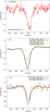 |
Fig. 9. Single snapshot of K Iλ7699, and the evolution of He I and Paβ lines in velocity space. |
Although the HRS spectrum is too noisy to directly reveal the Na D and Li Iλ6707 lines, spectra (especially those from the target fibre; i.e. without the sky subtraction) smoothed with gaussian functions of different widths, always show flux depression near the expected wavelength. However, similarly as observed by Herbig et al. (2003) and Szabó et al. (2021), the lithium line appears to be blueshifted, thus we likely detected the shell component dominating the entire line profile like in K Iλ7699.
The visual and NIR spectra contain only a few emission lines. The strongest is Hα and slightly weaker are those from the calcium IR triplet (Ca II IRT), as shown in Fig. 2ab. However, high-resolution SALT/HRS spectra revealed their P-Cygni nature (Fig. 10), commonly found in FUors. The highest wind velocities inferred from the blueshifted absorption components reach −400 km s−1 (Hα), and almost twice less in the calcium triplet.
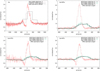 |
Fig. 10. Evolution of Hα and Ca II IRT in velocity space. |
The structure of Hα is likely variable, as inferred from comparison of the line profiles obtained by SPRAT and HRS. As these instruments have very different spectral resolutions, to enable direct comparison we downgraded resolution of the HRS spectrum (0.04 Å pix−1) to that of SPRAT (9.2 Å pix−1). The result shown in Figure 10 reveals that three years earlier (2020 December 21) the Hα line most likely showed the emission component only. This could be true if the absorption component was relatively weak or just moderate in comparison to the emission one, as observed in the spectrum of Gaia21bty (likely a FUor), obtained at the beginning of the outburst (Siwak et al. 2023).
Three spectra covering the calcium IR triplet, obtained within five days, reveal a strong variability for all three components. Both SpeX spectra show just a strongly redshifted emission. However, a more careful look reveals similar variations of all the three components within one day, which may be interpreted as a gradual evolution towards the shape observed four days later by HRS. The HRS spectrum reveals stronger emission component, but also previously unseen absorption component (both leading to the P-Cygni profile) in all but the first lines (Fig. 10). Based on the HRS spectrum resampled to the SpeX’s resolution, the absorption component was likely absent in the SpeX spectra. Thus, it appears that P-Cygni profile is not always present in Ca II IRT. Time-series observations obtained with a daily cadence are necessary to study this phenomenon, while the same conclusion is also applied to the Hα (see also in Powell et al. 2012).
We made similar comparisons for the He I 10830 (for this purpose the SpeX spectra were resampled to the lower SOFI’s resolution), where the line turned out to be the strongest in 2023 (Fig. 9). The variability of Paβ is more complex, as seen in the first spectrum taken by SOFI (2021 May 9), the line was undefined in the noisy continuum, but only later (2023) was it seen in absorption. In Gaia21bty, the two IR spectra taken early in the outburst showed the line first in emission and then (48 days later), probably equal to the continuum (Siwak et al. 2023). We note that the Paβ depth in the Gaia20bdk spectra is also variable, as inferred from the NOTCam and SpeX spectra, both offering practically the same resolutions. We also note that in both He I and Paβ, their blue and red wings extend to ±500 km s−1, noting that the blue ones are more affected by an extended wind absorption.
4. Conclusions
Gaia20bdk, a Class I member of relatively distant (3–3.6 kpc) Sh 2-301 star-forming region in Canis Major, started systematic brightening in late 2018. It became quickly obvious that both the brightening amplitude (from 3.9 in blue to 1.3 mag in the IR) and the rate may indicate a new FU Ori-type eruptive event. Literature studies have shown that the brightening process was similar to that observed for HBC 722. The CMDs show that the brightening did not occur along the extinction path; therefore, it can not be explained by extinction reduction in the line of sight. Our NIR spectra show all features typical for FUors, especially the CO-bandhead in absorption, triangular shape of H-band spectrum, and most of hydrogen and heavier elements in absorption. These data have definitively confirmed the FUor classification of the object. The Hα and Ca II IRT lines are showing P-Cygni profiles, with stronger emission components accompanied by weaker absorptions, are indicative of a high-velocity (up to −500 km s−1) disc wind. The shape of the Ca II IRT varies on a timescale of days, which is probably caused by non-uniform density of the inner disc wind.
The light curve plateau shows small-scale photometric variability. It is usually associated with disc flickering observed in other FUors and accreting objects. The longest variability component shows 1.8 yr quasi-periodicity and it was probably also present in the quiescence. If so, it would have been caused by variable extinction or a wind, which means that it originates in the outer disc environments rather than in the inner; thus, it would probably not be related with the eruptive event. The shorter 68–210 d significant signals are likely single oscillatory events, thus it would not meet the QPO definition. However, the wavelet spectrum suggests possible family of 10–40 d QPOs, which could originate in the inner disc at the place of the sharp temperature drop, such as that numerically predicted at 0.15 au in FU Ori by Zhu et al. (2020).
From the data gathered during the plateau, we constructed three SEDs. Models assuming the distance of 3.3 kpc, the inner disc radius 4 R⊙, and the stellar mass 2.67 M⊙ result in a disc luminosity of 133–165 L⊙ and a mass accretion rate of 1.2 − 1.8 × 10⁻⁵ M⊙ yr−1, which is typical for FUors. In practice, these values are invariant on the assumed distance (3–3.6 kpc) and the stellar mass (2.2–3.2 M⊙). Our best-fit models suggest rather small outer ‘active’ disc radius (0.3–0.4 au). Unfortunately, the AV value of 5.6–6.0 mag obtained from the NIR observations is not well reproduced by our disc models.
Further observing efforts are necessary to monitor the outburst behaviour and to resolve several inconsistencies raised above. The target is bright enough to make time-series spectroscopic and photometric observations for a range of further analyses, in particular the Doppler imaging of the inner disc atmosphere and the wind structure.
Due to the break in Gaia measurements of our target, to estimate this moment, we used the combined r-band light curve.
Although this parameter was determined above from our observations, we got much better results when we were fitting it, as the brightness of Gaia20bdk is still rising.
Although the logistic functions failed in their original application, they are good enough for removing the general brightness increase associated with the outburst.
We also considered other values, but we always came to the conclusion that they do not lead to more satisfactory results.
Acknowledgments
We acknowledge support from the ESA PRODEX contract nr. 4000132054. We acknowledge the Hungarian National Research, Development and Innovation Office grant OTKA FK 146023. G. M. and Zs. N. were supported by the János Bolyai Research Scholarship of the Hungarian Academy of Sciences. G.M. acknowledges support from the European Union’s Horizon 2020 research and innovation programme under grant agreement No. 101004141. This project has received funding from the European Research Council (ERC) under the European Union’s Horizon 2020 research and innovation programme under grant agreement No 716155 (SACCRED). This work was also supported by the NKFIH excellence grant TKP2021-NKTA-64. E.F. acknowledges financial support from the project PRIN-INAF 2019 ‘Spectroscopically Tracing the Disc Dispersal Evolution (STRADE)’. Zs.M.Sz. acknowledges funding from a St Leonards scholarship from the University of St Andrews. For the purpose of open access, the author has applied a Creative Commons Attribution (CC BY) licence to any Author Accepted Manuscript version arising. Member of the International Max Planck Research School (IMPRS) for Astronomy and Astrophysics at the Universities of Bonn and Cologne. Based on observations made with the Nordic Optical Telescope, owned in collaboration by the University of Turku and Aarhus University, and operated jointly by Aarhus University, the University of Turku and the University of Oslo, representing Denmark, Finland and Norway, the University of Iceland and Stockholm University at the Observatorio del Roque de los Muchachos, La Palma, Spain, of the Instituto de Astrofisica de Canarias. The research leading to these results has received funding from the European Community’s Horizon 2020 Programme (H2020/2021-2024) under grant agreement number 101004719 (ORP). Based on observations made with ESO Telescopes at the La Silla and Paranal Observatories under programme ID: 105.203T.001. Based on data obtained from the ESO Science Archive Facility. This work is based in part on data obtained with the NASA Infrared Telescope Facility, which is operated by the University of Hawaii under a contract with the National Aeronautics and Space Administration. The authors wish to recognize and acknowledge the very significant cultural role and reverence that the summit of Maunakea has always had within the indigenous Hawaiian community. We are most fortunate to have the opportunity to conduct observations from this mountain. This paper uses observations made at the South African Astronomical Observatory (SAAO). Some of the observations reported in this paper were obtained with the Southern African Large Telescope (SALT). Polish participation in SALT is funded by grant No. MNiSW DIR/WK/2016/07. This publication makes use of data products from the Two Micron All Sky Survey, which is a joint project of the University of Massachusetts and the Infrared Processing and Analysis Center/California Institute of Technology, funded by the National Aeronautics and Space Administration and the National Science Foundation. This publication makes use of data products from the Wide-field Infrared Survey Explorer, which is a joint project of the University of California, Los Angeles, and the Jet Propulsion Laboratory/California Institute of Technology, funded by the National Aeronautics and Space Administration. This research has made use of the NASA/IPAC Infrared Science Archive, which is funded by the National Aeronautics and Space Administration and operated by the California Institute of Technology. We acknowledge ESA Gaia, DPAC and the Photometric Science Alerts Team (http://gsaweb.ast.cam.ac.uk/alerts). The Pan-STARRS1 Surveys (PS1) and the PS1 public science archive have been made possible through contributions by the Institute for Astronomy, the University of Hawaii, the Pan-STARRS Project Office, the Max-Planck Society and its participating institutes, the Max Planck Institute for Astronomy, Heidelberg and the Max Planck Institute for Extraterrestrial Physics, Garching, The Johns Hopkins University, Durham University, the University of Edinburgh, the Queen’s University Belfast, the Harvard-Smithsonian Center for Astrophysics, the Las Cumbres Observatory Global Telescope Network Incorporated, the National Central University of Taiwan, the Space Telescope Science Institute, the National Aeronautics and Space Administration under Grant No. NNX08AR22G issued through the Planetary Science Division of the NASA Science Mission Directorate, the National Science Foundation Grant No. AST-1238877, the University of Maryland, Eotvos Lorand University (ELTE), the Los Alamos National Laboratory, and the Gordon and Betty Moore Foundation. The national facility capability for SkyMapper has been funded through ARC LIEF grant LE130100104 from the Australian Research Council, awarded to the University of Sydney, the Australian National University, Swinburne University of Technology, the University of Queensland, the University of Western Australia, the University of Melbourne, Curtin University of Technology, Monash University and the Australian Astronomical Observatory. SkyMapper is owned and operated by The Australian National University’s Research School of Astronomy and Astrophysics. The survey data were processed and provided by the SkyMapper Team at ANU. The SkyMapper node of the All-Sky Virtual Observatory (ASVO) is hosted at the National Computational Infrastructure (NCI). Development and support of the SkyMapper node of the ASVO has been funded in part by Astronomy Australia Limited (AAL) and the Australian Government through the Commonwealth’s Education Investment Fund (EIF) and National Collaborative Research Infrastructure Strategy (NCRIS), particularly the National eResearch Collaboration Tools and Resources (NeCTAR) and the Australian National Data Service Projects (ANDS). This research has made use of the Spanish Virtual Observatory (http://svo.cab.inta-csic.es) supported from Ministerio de Ciencia e Innovación through grant PID2020-112949GB-I00. This paper uses observations made at the Mount Suhora Astronomical Observatory, Poland. The operation of the RC80 telescope at Konkoly Observatory has been supported by the GINOP 2.3.2-15-2016-00033 grant of the National Research, Development and Innovation Office (NKFIH) funded by the European Union. Based on the observations made with the Liverpool Telescope operated on the island of La Palma by Liverpool John Moores University in the Spanish Observatorio del Roque de los Muchachos of the Instituto de Astrofisica de Canarias with financial support from the UK Science and Technology Facilities Council. The Liverpool Telescope is operated on the island of La Palma by Liverpool John Moores University in the Spanish Observatorio del Roque de los Muchachos of the Instituto de Astrofisica de Canarias with financial support from the UK Science and Technology Facilities Council. This paper made use of NASA’s Astrophysics Data System (ADS) Bibliographic Services. Special thanks are also due to an anonymous referee for highly useful suggestions and comments on the previous version of the paper.
References
- Ábrahám, P., Juhász, A., Dullemond, C. P., et al. 2009, Nature, 459, 224 [Google Scholar]
- Ábrahám, P., Chen, L., Kóspál, Á., et al. 2019, ApJ, 887, 156 [Google Scholar]
- Acosta-Pulido, J. A., Kun, M., Ábrahám, P., et al. 2007, AJ, 133, 2020 [NASA ADS] [CrossRef] [Google Scholar]
- Andrews, S. M., Rothberg, B., & Simon, T. 2004, ApJ, 610, L45 [NASA ADS] [CrossRef] [Google Scholar]
- Ashraf, M., Jose, J., Lee, H.-G., et al. 2024, MNRAS, 527, 11651 [Google Scholar]
- Audard, M., Ábrahám, P., Dunham, M. M., et al. 2014, in Protostars and Planets VI, eds. H. Beuther, R. S. Klessen, C. P. Dullemond, & T. Henning, 387 [Google Scholar]
- Baek, G., Pak, S., Green, J. D., et al. 2015, AJ, 149, 11 [NASA ADS] [CrossRef] [Google Scholar]
- Bailer-Jones, C. A. L., Rybizki, J., Fouesneau, M., Demleitner, M., & Andrae, R. 2021, AJ, 161, 147 [Google Scholar]
- Bell, K. R., Lin, D. N. C., Hartmann, L. W., & Kenyon, S. J. 1995, ApJ, 444, 376 [NASA ADS] [CrossRef] [Google Scholar]
- Bellm, E. C., Kulkarni, S. R., Graham, M. J., et al. 2019, PASP, 131, 018002 [Google Scholar]
- Bessell, M. S., & Brett, J. M. 1988, PASP, 100, 1134 [Google Scholar]
- Cantat-Gaudin, T., Anders, F., Castro-Ginard, A., et al. 2020, A&A, 640, A1 [NASA ADS] [CrossRef] [EDP Sciences] [Google Scholar]
- Cardelli, J. A., Clayton, G. C., & Mathis, J. S. 1989, ApJ, 345, 245 [Google Scholar]
- Carvalho, A., Hillenbrand, L., Seebeck, J., & Covey, K. 2024, ApJ, 971, 44 [NASA ADS] [Google Scholar]
- Chambers, K. C., Magnier, E. A., Metcalfe, N., et al. 2016, arXiv e-prints [arXiv:1612.05560] [Google Scholar]
- Cieza, L. A., Casassus, S., Tobin, J., et al. 2016, Nature, 535, 258 [Google Scholar]
- Connelley, M. S., & Reipurth, B. 2018, ApJ, 861, 145 [NASA ADS] [CrossRef] [Google Scholar]
- Contreras Peña, C., Lucas, P. W., Kurtev, R., et al. 2017, MNRAS, 465, 3039 [Google Scholar]
- Contreras Peña, C., Naylor, T., & Morrell, S. 2019, MNRAS, 486, 4590 [CrossRef] [Google Scholar]
- Contreras Peña, C., Ashraf, M., Lee, J.-E., et al. 2023, JKAS, 56, 253 [Google Scholar]
- Contreras Peña, C., Lucas, P. W., Guo, Z., & Smith, L. 2024, MNRAS, 528, 1823 [Google Scholar]
- Crause, L. A., Sharples, R. M., Bramall, D. G., et al. 2014, in Ground-based and Airborne Instrumentation for Astronomy V, eds. S. K. Ramsay, I. S. McLean, & H. Takami, SPIE Conf. Ser., 9147, 91476T [NASA ADS] [Google Scholar]
- Cushing, M. C., Vacca, W. D., & Rayner, J. T. 2004, PASP, 116, 362 [NASA ADS] [CrossRef] [Google Scholar]
- Cutri, R. M., Skrutskie, M. F., van Dyk, S., et al. 2003, VizieR Online Data Catalog, II/246 [Google Scholar]
- Drew, J. E., Gonzalez-Solares, E., Greimel, R., et al. 2014, MNRAS, 440, 2036 [Google Scholar]
- Dutra, C. M., Bica, E., Soares, J., & Barbuy, B. 2003, A&A, 400, 533 [NASA ADS] [CrossRef] [EDP Sciences] [Google Scholar]
- Fiorellino, E., Tychoniec, Ł., Cruz-Sáenz de Miera, F., et al. 2023, ApJ, 944, 135 [NASA ADS] [CrossRef] [Google Scholar]
- Fiorellino, E., Ábrahám, P., Kóspál, Á., et al. 2024, A&A, 686, A160 [NASA ADS] [CrossRef] [EDP Sciences] [Google Scholar]
- Fischer, W. J., Hillenbrand, L. A., Herczeg, G. J., et al. 2023, in Protostars and Planets VII, eds. S. Inutsuka, Y. Aikawa, T. Muto, et al., ASP Conf. Ser., 534, 355 [NASA ADS] [Google Scholar]
- Foster, G. 1996, AJ, 112, 1709 [NASA ADS] [CrossRef] [Google Scholar]
- Gaia Collaboration (Prusti, T., et al.) 2016, A&A, 595, A1 [NASA ADS] [CrossRef] [EDP Sciences] [Google Scholar]
- Gaia Collaboration (Vallenari, A., et al.) 2023, A&A, 674, A1 [NASA ADS] [CrossRef] [EDP Sciences] [Google Scholar]
- Green, J. D., Robertson, P., Baek, G., et al. 2013, ApJ, 764, 22 [Google Scholar]
- Green, G. M., Schlafly, E., Zucker, C., Speagle, J. S., & Finkbeiner, D. 2019, ApJ, 887, 93 [NASA ADS] [CrossRef] [Google Scholar]
- Guo, Z., Lucas, P. W., Contreras Peña, C., et al. 2020, MNRAS, 492, 294 [NASA ADS] [CrossRef] [Google Scholar]
- Guo, Z., Lucas, P. W., Contreras Pena, C., et al. 2021, MNRAS, 504, 830 [NASA ADS] [CrossRef] [Google Scholar]
- Guo, Z., Lucas, P. W., Kurtev, R., et al. 2024a, MNRAS, 528, 1769 [NASA ADS] [CrossRef] [Google Scholar]
- Guo, Z., Lucas, P. W., Kurtev, R. G., et al. 2024b, MNRAS, 529, L115 [Google Scholar]
- Hanaoka, M., Kaneda, H., Suzuki, T., et al. 2019, PASJ, 71, 6 [NASA ADS] [CrossRef] [Google Scholar]
- Hartmann, L., & Kenyon, S. J. 1996, ARA&A, 34, 207 [NASA ADS] [CrossRef] [Google Scholar]
- Heinze, A. N., Tonry, J. L., Denneau, L., et al. 2018, AJ, 156, 241 [Google Scholar]
- Henden, A. A., Levine, S., Terrell, D., & Welch, D. L. 2015, Am. Astron. Soc. Meeting Abstr., 225, 336.16 [Google Scholar]
- Henden, A. A., Templeton, M., Terrell, D., et al. 2016, VizieR Online Data Catalog, II/336 [Google Scholar]
- Herbig, G. H. 1977, ApJ, 217, 693 [NASA ADS] [CrossRef] [Google Scholar]
- Herbig, G. H. 1989, Eur. Southern Obs. Conf. Workshop Proc., 33, 233 [NASA ADS] [Google Scholar]
- Herbig, G. H., Petrov, P. P., & Duemmler, R. 2003, ApJ, 595, 384 [Google Scholar]
- Herczeg, G. J., Dong, S., Shappee, B. J., et al. 2016, ApJ, 831, 133 [NASA ADS] [Google Scholar]
- Hillenbrand, L. A., Contreras Peña, C., Morrell, S., et al. 2018, ApJ, 869, 146 [NASA ADS] [CrossRef] [Google Scholar]
- Hillenbrand, L. A., Miller, A., Carpenter, J. M., et al. 2019a, ApJ, 874, 82 [NASA ADS] [Google Scholar]
- Hillenbrand, L. A., Reipurth, B., Connelley, M., Cutri, R. M., & Isaacson, H. 2019b, AJ, 158, 240 [NASA ADS] [CrossRef] [Google Scholar]
- Hillenbrand, L. A., De, K., Hankins, M., et al. 2021, AJ, 161, 220 [NASA ADS] [CrossRef] [Google Scholar]
- Hillenbrand, L. A., Carvalho, A., van Roestel, J., & De, K. 2023, ApJ, 958, L27 [NASA ADS] [CrossRef] [Google Scholar]
- Hodapp, K. W., Denneau, L., Tucker, M., et al. 2020, AJ, 160, 164 [NASA ADS] [CrossRef] [Google Scholar]
- Hodgkin, S. T., Harrison, D. L., Breedt, E., et al. 2021, A&A, 652, A76 [NASA ADS] [CrossRef] [EDP Sciences] [Google Scholar]
- Holoien, T. W. S., Prieto, J. L., Stanek, K. Z., et al. 2014, ApJ, 785, L35 [NASA ADS] [CrossRef] [Google Scholar]
- Hou, L. G., & Han, J. L. 2014, A&A, 569, A125 [NASA ADS] [CrossRef] [EDP Sciences] [Google Scholar]
- Hubbard, A. 2017a, ApJ, 840, 6 [Google Scholar]
- Hubbard, A. 2017b, ApJ, 840, L5 [NASA ADS] [CrossRef] [Google Scholar]
- Hunt, E. L., & Reffert, S. 2023, A&A, 673, A114 [NASA ADS] [CrossRef] [EDP Sciences] [Google Scholar]
- Kenyon, S. J., Kolotilov, E. A., Ibragimov, M. A., & Mattei, J. A. 2000, ApJ, 531, 1028 [NASA ADS] [CrossRef] [Google Scholar]
- Kharchenko, N. V., Piskunov, A. E., Schilbach, E., Röser, S., & Scholz, R. D. 2013, A&A, 558, A53 [NASA ADS] [CrossRef] [EDP Sciences] [Google Scholar]
- Kniazev, A. Y., Gvaramadze, V. V., & Berdnikov, L. N. 2016, MNRAS, 459, 3068 [NASA ADS] [CrossRef] [Google Scholar]
- Kniazev, A. Y., Gvaramadze, V. V., & Berdnikov, L. N. 2017, in Stars: From Collapse to Collapse, eds. Y. Y. Balega, D. O. Kudryavtsev, I. I. Romanyuk, & I. A. Yakunin, ASP Conf. Ser., 510, 480 [NASA ADS] [Google Scholar]
- Kóspál, Á., Ábrahám, P., Acosta-Pulido, J. A., et al. 2016, A&A, 596, A52 [NASA ADS] [CrossRef] [EDP Sciences] [Google Scholar]
- Kóspál, Á., Ábrahám, P., Carmona, A., et al. 2020, ApJ, 895, L48 [CrossRef] [Google Scholar]
- Kóspál, Á., Ábrahám, P., Diehl, L., et al. 2023, ApJ, 945, L7 [CrossRef] [Google Scholar]
- Kuhn, M. A., de Souza, R. S., Krone-Martins, A., et al. 2021, ApJS, 254, 33 [NASA ADS] [CrossRef] [Google Scholar]
- Kuhn, M. A., Hillenbrand, L. A., Connelley, M. S., et al. 2024, MNRAS, 529, 2630 [CrossRef] [Google Scholar]
- Kun, M., Ábrahám, P., Acosta Pulido, J. A., Moór, A., & Prusti, T. 2019, MNRAS, 483, 4424 [NASA ADS] [CrossRef] [Google Scholar]
- Liu, H., Herczeg, G. J., Johnstone, D., et al. 2022, ApJ, 936, 152 [NASA ADS] [CrossRef] [Google Scholar]
- Lykou, F., Ábrahám, P., Chen, L., et al. 2022, A&A, 663, A86 [NASA ADS] [CrossRef] [EDP Sciences] [Google Scholar]
- Magakian, T. Y., Movsessian, T. A., Andreasyan, H. R., Moiseev, A. V., & Uklein, R. I. 2023, A&A, 675, A79 [NASA ADS] [CrossRef] [EDP Sciences] [Google Scholar]
- Magnier, E. A., Chambers, K. C., Flewelling, H. A., et al. 2020, ApJS, 251, 3 [NASA ADS] [CrossRef] [Google Scholar]
- Mainzer, A., Bauer, J., Grav, T., et al. 2011, ApJ, 731, 53 [Google Scholar]
- Marton, G., Tóth, L. V., Paladini, R., et al. 2016, MNRAS, 458, 3479 [Google Scholar]
- Masci, F. J., Laher, R. R., Rusholme, B., et al. 2019, PASP, 131, 018003 [Google Scholar]
- Meyer, M. R., Calvet, N., & Hillenbrand, L. A. 1997, AJ, 114, 288 [Google Scholar]
- Molyarova, T., Akimkin, V., Semenov, D., et al. 2018, ApJ, 866, 46 [NASA ADS] [CrossRef] [Google Scholar]
- Moorwood, A., Cuby, J. G., & Lidman, C. 1998, The Messenger, 91, 9 [Google Scholar]
- Muzerolle, J., Megeath, S. T., Flaherty, K. M., et al. 2005, ApJ, 620, L107 [CrossRef] [Google Scholar]
- Nagy, Z., Park, S., Ábrahám, P., et al. 2023, MNRAS, 524, 3344 [NASA ADS] [CrossRef] [Google Scholar]
- Ninan, J. P., Ojha, D. K., Baug, T., et al. 2015, ApJ, 815, 4 [NASA ADS] [CrossRef] [Google Scholar]
- Onken, C. A., Wolf, C., Bessell, M. S., et al. 2019, PASA, 36, e033 [Google Scholar]
- Onken, C. A., Wolf, C., Bessell, M. S., et al. 2024, PASA, 41, e061 [NASA ADS] [CrossRef] [Google Scholar]
- Pandey, R., Sharma, S., Dewangan, L. K., et al. 2022, ApJ, 926, 25 [NASA ADS] [CrossRef] [Google Scholar]
- Park, S., Kóspál, Á., Cruz-Sáenz de Miera, F., et al. 2021, ApJ, 923, 171 [NASA ADS] [CrossRef] [Google Scholar]
- Piascik, A. S., Steele, I. A., Bates, S. D., et al. 2014, in Ground-based and Airborne Instrumentation for Astronomy V, eds. S. K. Ramsay, I. S. McLean, & H. Takami, SPIE Conf. Ser., 9147, 91478H [NASA ADS] [Google Scholar]
- Powell, S. L., Irwin, M., Bouvier, J., & Clarke, C. J. 2012, MNRAS, 426, 3315 [NASA ADS] [CrossRef] [Google Scholar]
- Press, W. H. 1978, Comm. Mod. Phys., Part C - Comm. Astrophys., 7, 103 [NASA ADS] [Google Scholar]
- Rayner, J. T., Toomey, D. W., Onaka, P. M., et al. 2003, PASP, 115, 362 [NASA ADS] [CrossRef] [Google Scholar]
- Scaringi, S., Maccarone, T. J., Kording, E., et al. 2015, Sci. Adv., 1, e1500686 [NASA ADS] [CrossRef] [Google Scholar]
- Shingles, L., Smith, K. W., Young, D. R., et al. 2021, Transient Name Server AstroNote, 7, 1 [NASA ADS] [Google Scholar]
- Sicilia-Aguilar, A., Oprandi, A., Froebrich, D., et al. 2017, A&A, 607, A127 [NASA ADS] [CrossRef] [EDP Sciences] [Google Scholar]
- Siess, L., Dufour, E., & Forestini, M. 2000, A&A, 358, 593 [Google Scholar]
- Siwak, M., Ruciński, S. M., Matthews, J. M., et al. 2013, MNRAS, 432, 194 [NASA ADS] [CrossRef] [Google Scholar]
- Siwak, M., Winiarski, M., Ogłoza, W., et al. 2018, A&A, 618, A79 [NASA ADS] [CrossRef] [EDP Sciences] [Google Scholar]
- Siwak, M., Ogłoza, W., & Krzesiński, J. 2020, A&A, 644, A135 [NASA ADS] [CrossRef] [EDP Sciences] [Google Scholar]
- Siwak, M., Hillenbrand, L. A., Kóspál, Á., et al. 2023, MNRAS, 524, 5548 [NASA ADS] [CrossRef] [Google Scholar]
- Skrutskie, M. F., Cutri, R. M., Stiening, R., et al. 2006, AJ, 131, 1163 [NASA ADS] [CrossRef] [Google Scholar]
- Smith, K. W., Smartt, S. J., Young, D. R., et al. 2020, PASP, 132, 085002 [Google Scholar]
- Steele, I. A., Smith, R. J., Rees, P. C., et al. 2004, in Ground-based Telescopes, eds. J. Oschmann, & M. Jacobus, SPIE Conf. Ser., 5489, 679 [NASA ADS] [CrossRef] [Google Scholar]
- Stetson, P. B. 1987, PASP, 99, 191 [Google Scholar]
- Szabó, Z. M., Kóspál, Á., Ábrahám, P., et al. 2021, ApJ, 917, 80 [CrossRef] [Google Scholar]
- Szabó, Z. M., Kóspál, Á., Ábrahám, P., et al. 2022, ApJ, 936, 64 [CrossRef] [Google Scholar]
- Szegedi-Elek, E., Ábrahám, P., Wyrzykowski, Ł., et al. 2020, ApJ, 899, 130 [Google Scholar]
- Tonry, J. L., Denneau, L., Heinze, A. N., et al. 2018, PASP, 130, 064505 [Google Scholar]
- Tran, V., De, K., & Hillenbrand, L. 2024, MNRAS, 530, 2076 [NASA ADS] [CrossRef] [Google Scholar]
- Vacca, W. D., Cushing, M. C., & Rayner, J. T. 2003, PASP, 115, 389 [NASA ADS] [CrossRef] [Google Scholar]
- Waters, C. Z., Magnier, E. A., Price, P. A., et al. 2020, ApJS, 251, 4 [NASA ADS] [CrossRef] [Google Scholar]
- Wiebe, D. S., Molyarova, T. S., Akimkin, V. V., Vorobyov, E. I., & Semenov, D. A. 2019, MNRAS, 485, 1843 [Google Scholar]
- Wright, E. L., Eisenhardt, P. R. M., Mainzer, A. K., et al. 2010, AJ, 140, 1868 [Google Scholar]
- Yoon, S.-Y., Lee, J.-E., Lee, S., et al. 2021, ApJ, 919, 116 [NASA ADS] [CrossRef] [Google Scholar]
- Zechmeister, M., & Kürster, M. 2009, A&A, 496, 577 [CrossRef] [EDP Sciences] [Google Scholar]
- Zhu, Z., Hartmann, L., Calvet, N., et al. 2007, ApJ, 669, 483 [NASA ADS] [CrossRef] [Google Scholar]
- Zhu, Z., Jiang, Y.-F., & Stone, J. M. 2020, MNRAS, 495, 3494 [NASA ADS] [CrossRef] [Google Scholar]
Appendix A: Photometric data for Gaia20bdk
Optical pre-outburst photometry of Gaia20bdk, with only our own photometric determinations extracted from public-domain fits images listed.
Near-infrared and optical photometry of Gaia20bdk gathered in this study during the outburst.
Appendix B: Line identification in the near–infrared spectra.
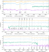 |
Fig. B.1. Lines identified in the near-infrared spectra. In the case of H&K bands, unidentified lines (or with uncertain identification) from the bracket and CO series are labelled with a smaller font and a question mark. Note: the large fraction of positive results we owe to the IRTF/SpeX spectra. In the H-band, the position of CO series is marked by solid black lines, while the bracket series and metal lines by the dashed lines. |
All Tables
Optical pre-outburst photometry of Gaia20bdk, with only our own photometric determinations extracted from public-domain fits images listed.
Near-infrared and optical photometry of Gaia20bdk gathered in this study during the outburst.
All Figures
|
Fig. 1. Combined griJHKS light curves of Gaia20bdk obtained by several ground-based surveys and telescopes, and G, W1, and W2 light curves obtained by Gaia and (NEO)WISE space telescopes, as described in Sects. 2.1 and 2.2. The first JHKS data points from 1999 Feb 1 obtained by 2MASS were shifted forward by exactly 11 years, so they appear on this plot on 2010 Feb 1. |
| In the text | |
|
Fig. 2. Low-resolution LT/SPRAT spectrum (panel a), and the NTT/SOFI (2021 May 9) and the IRTF/SpeX (2023 December 3) low- and medium-resolution flux-calibrated spectra of Gaia20bdk (panel b). The grey-shaded areas in this panel demarcate regions strongly affected by telluric lines. The IRTF spectrum and photometry were shifted up by 3 × 10⁻¹⁵ erg cm−1 s−1 Å−1 for clarity. Only the major spectral lines and bands characteristic of FUors are indicated. Telluric absorption bands were not removed from the visual spectrum. |
| In the text | |
|
Fig. 3. Analytical fits of logistic function to the best sampled grGW1W2 light curves (panel a). Second panel shows the residuals after subtraction of respective logistic functions. |
| In the text | |
|
Fig. 4. ATLAS o-band light curve obtained during the plateau, with the slow brightening trend removed (panel a). The second panel shows Fourier spectrum (black line) in the log-log scale, calculated from the o-band data taken during the plateau and transformed to normalised flux unit. The flickering noise nature (af ∼ f−1/2) of these oscillations is indicated by the two parallel green dashed lines, while the amplitude errors are represented by blue dots. Third panel (c) shows respective WWZ spectrum. The major edge effects lie outside of the white dashed lines. The WWZ power is expressed in colours, as shown in the right label. |
| In the text | |
|
Fig. 5. CMDs in the optical and IR part of the spectrum. The (NEO)WISE data are colour-coded: blue represents the quiescence, yellow: the rising branch and red: the plateau. The bottom line shows two diagrams computed from the detrended ZTF and RC80 gri data taken during the plateau only. |
| In the text | |
|
Fig. 6. J − H vs. H − KS colour-colour diagram prepared from pre-outburst (2MASS and Pandey et al. 2022) & outburst (SOFI, NOT, IRTF) data of Gaia20bdk. The squares represent zero age main sequence (ZAMS) stars, while the open circles show giant branch (GB) stars (Bessell & Brett 1988). The black line is the locus of unreddened CTTS (Meyer et al. 1997). The two parallel lines formed from pluses represent the reddening path; the step represents the reddening by additional 1 mag in AV. |
| In the text | |
|
Fig. 7. Pre-outburst SED suggesting either flat spectrum or Class I membership (panel a). The same panel shows results of the dereddened quiescent data modelling. Position of the star in the H-R diagram based on modelling results (panels b&c); the one obtained with the assumption of the optimal temperature (5300 K) and distance (3.3 kpc) is indicated by the largest dot. The size of the dot fairly well represent the uncertainty in L* and R* caused by uncertainty in distance (3.0–3.6 kpc); Similar size should be applied to the two small dots to indicate uncertainties. |
| In the text | |
|
Fig. 8. Results from disc modelling of SOFI, NOTCam and SpeX data (i.e. Epoch 1, 2, and 3, respectively), as shown in Table 1. |
| In the text | |
|
Fig. 9. Single snapshot of K Iλ7699, and the evolution of He I and Paβ lines in velocity space. |
| In the text | |
|
Fig. 10. Evolution of Hα and Ca II IRT in velocity space. |
| In the text | |
|
Fig. B.1. Lines identified in the near-infrared spectra. In the case of H&K bands, unidentified lines (or with uncertain identification) from the bracket and CO series are labelled with a smaller font and a question mark. Note: the large fraction of positive results we owe to the IRTF/SpeX spectra. In the H-band, the position of CO series is marked by solid black lines, while the bracket series and metal lines by the dashed lines. |
| In the text | |
Current usage metrics show cumulative count of Article Views (full-text article views including HTML views, PDF and ePub downloads, according to the available data) and Abstracts Views on Vision4Press platform.
Data correspond to usage on the plateform after 2015. The current usage metrics is available 48-96 hours after online publication and is updated daily on week days.
Initial download of the metrics may take a while.