| Issue |
A&A
Volume 678, October 2023
|
|
|---|---|---|
| Article Number | A88 | |
| Number of page(s) | 18 | |
| Section | Interstellar and circumstellar matter | |
| DOI | https://doi.org/10.1051/0004-6361/202347063 | |
| Published online | 11 October 2023 | |
Brightness and mass accretion rate evolution during the 2022 burst of EX Lupi★
1
Konkoly Observatory, HUN-REN Research Centre for Astronomy and Earth Sciences,
Konkoly-Thege Miklós út 15-17,
1121
Budapest, Hungary
2
CSFK, MTA Centre of Excellence,
Konkoly-Thege Miklós út 15-17,
1121
Budapest, Hungary
3
Institut de Recherche en Astrophysique et Planétologie, Université de Toulouse,
UT3-PS, OMP, CNRS, 9 av. du Colonel-Roche,
31028
Toulouse Cedex 4, France
e-mail: fernando.cruz-saenz@irap.omp.eu
4
ELTE Eötvös Loránd University, Institute of Physics,
Pázmány Péter sétány 1/A,
1117
Budapest, Hungary
5
Max Planck Institute for Astronomy,
Königstuhl 17,
69117
Heidelberg, Germany
6
European Southern Observatory,
Karl-Schwarzschild-Strasse 2,
85748
Garching bei München, Germany
7
Department of Astronomy & Institute for Astrophysical Research, Boston University,
725 Commonwealth Avenue,
Boston, MA
02215, USA
8
INAF – Osservatorio Astronomico di Capodimonte,
via Moiariello 16,
80131
Napoli, Italy
9
INAF – Osservatorio Astronomico di Roma,
Via di Frascati 33,
00078
Monte Porzio Catone, Italy
10
SUPA, School of Science and Engineering, University of Dundee,
Nethergate, Dundee
DD1 4HN, UK
11
Department of Physics, Texas State University,
749 N Comanche Street,
San Marcos, TX
78666, USA
12
Max Planck Institute for Radioastronomy,
Auf dem Hügel 69,
53121
Bonn, Germany
13
SUPA, School of Physics and Astronomy, University of St Andrews,
North Haugh,
St Andrews,
KY16 9SS, UK
Received:
31
May
2023
Accepted:
3
August
2023
Context. EX Lupi is the prototype by which EXor-type outbursts have been defined. It has experienced multiple accretion-related bursts and outbursts throughout the past decades, and the study of these events has greatly extended our knowledge about their effects. Notably, this star experienced a new burst in 2022.
Aims. We aim to investigate whether the recent brightening was caused by temporarily increased accretion or by a brief decrease in the extinction and study the evolution of the EX Lupi system throughout this event.
Methods. We used multi-band photometry to create color-color and color-magnitude diagrams to exclude the possibility that the brightening could be explained by a decrease in extinction. We obtained spectra using the X-shooter instrument of the Very Large Telescope (VLT) to determine the Lacc and Ṁacc during the peak of the burst and after its return to quiescence using two different methods: empirical relationships between line luminosity and Lacc, and a slab model of the whole spectrum. We examined the 130-yr light curve of EX Lupi to provide statistics on the number of outbursts experienced during this period of time.
Results. Our analysis of the data taken during the 2022 burst confirmed that a change in extinction is not responsible for the brightening. Our two approaches in calculating the Ṁacc were in agreement and resulted in values that are two orders of magnitude above what had previously been estimated for EX Lupi using only a couple of individual emission lines, thus suggesting that EX Lupi is a strong accretor even when in quiescence. We determined that in 2022 March, the Ṁacc increased by a factor of seven with respect to the quiescent level. We also found hints that even though the Ṁacc had returned to near pre-outburst levels, certain physical properties of the gas (i.e., temperature and density) had not returned to the quiescent values.
Conclusions. We found that the mass accreted during this three-month event was 0.8 lunar masses, which is approximately half of what is accreted during a year of quiescence. We calculated that if EX Lupi remains as active as it has been for the past 130 yr, during which it has experienced at least three outbursts and ten bursts, then it will deplete the mass of its circumstellar material in less than 160 000 yr.
Key words: stars: individual: EX Lupi / stars: protostars / stars: formation / accretion, accretion disks
© The Authors 2023
 Open Access article, published by EDP Sciences, under the terms of the Creative Commons Attribution License (https://creativecommons.org/licenses/by/4.0), which permits unrestricted use, distribution, and reproduction in any medium, provided the original work is properly cited.
This article is published in open access under the Subscribe to Open model. Subscribe to A&A to support open access publication.
1 Introduction
Over the past 130 yr, EX Lupi has experienced at least three large outbursts (1944, 1955, and 2008) and more than a dozen smaller bursts (see Fig. 1 for the light curve and references). This star has been taken as the prototype of eruptive young stars that experience outbursts of 2–5 magnitudes lasting from a few months up to a year (EXors; Herbig 1989). Together with their longer and more powerful counterparts (FUors), EXors represent the most dramatic cases of variability in low-mass young stellar objects (Hartmann & Kenyon 1996; Audard et al. 2014; Fischer et al. 2023). Both types of events are caused by a sudden increase of the mass accretion rate (Ṁacc) from 10−10−10−8 M⊙ yr−1 in quiescence to 10−6−10−4 M⊙ yr−1 during outburst, resulting in an increase of their bolometric luminosity by up to two orders of magnitude. These accretion-related events can be detected via a 2–5 mag brightening in optical and/or near-infrared photometric bands. Recently, Fischer et al. (2023) proposed an additional classification for the accretion-related events. They classify the events when a young star brightens by 1–2.5 magnitudes for at least a week and for as long as a year as “bursts”, whereas they classify events that brighten by 2.5–6 magnitudes for many years to decades as “outbursts”.
EXors can present both bursts and outbursts, and, due to their short durations, these events can occur repeatedly (Herbig 1989; Audard et al. 2014). For example, V1118 Ori has experienced at least five outbursts in the last 30 yr (Giannini et al. 2020), ASASSN-13db has gone through one burst and one outburst since its discovery in 2013 (Sicilia-Aguilar et al. 2017), VY Tau experienced 14 outbursts between 1940 and 1970 (Herbig 1977), and, as mentioned above, EX Lupi has experienced multiple bursts and outbursts in the past 130 yr (Fig. 1). Indeed, the two latest identified EXors, namely, Gaia19fct (Hillenbrand 2019; Park et al. 2022) and Gaia20eae (Ghosh et al. 2022; Cruz-Sáenz de Miera et al. 2022) also show recurring bursts.
Historically, the discovery and monitoring of similar bursts in T Tauri stars was rare and accidental. However, in recent years, the availability of all-sky monitoring and time-series surveys operating at optical or infrared wavelengths have been very sensitive to new bursts, thus adding to the amount of known events. This increased quantity of bursts now makes possible the further evaluation of the astrophysical significance of such bursts in the formation of low-mass stellar systems, including their contribution to the buildup of the protostar and their impact on disk structure, material, and chemistry. Therefore, to properly evaluate their effects, we need to take into account that while such bursts are less energetic than the outbursts, they have a shorter duty cycle and may produce significant cumulative effects that could impact the observations (Claes et al. 2022) and our overall interpretation of how disks evolve (Manara et al. 2023).
In 2022 March, Zhou & Herczeg (2022) and Kóspál et al. (2022) reported that EX Lupi was brightening again, based on ɡ band magnitudes from the All-Sky Automated Survey for Supernovae (ASAS-SN) survey as well as on dedicated optical and near-infrared monitoring. By 2022 March 10, the source had become 1.6 mag brighter than the previous baseline in 2021. An analysis of multi-band photometry taken during the early stages of the outbursts suggested that the brightening was not due to a decrease in the extinction but instead to an increase of the Ṁacc. We performed a multi-facility campaign using REM, LCOGT, VLT/X-shooter, VLTI/MATISSE, and ALMA observations in order to characterize the multi-band photometric evolution of the 2021 event, study the elevated mass accretion, and learn about the post-burst chemical and mineralogical impact on the disk. Among the main astrophysical questions, our aims were also to verify whether the magnetospheric accretion model is suitable to describe such bursts and outbursts, investigate the possible role of instabilities in triggering the brightenings, and test if the bursts would fit into a general picture that connects routine variability with the FUor-type outbursts (e.g., Liu et al. 2022). In this work, we report on the photometric monitoring and the UV, optical, and near-infrared spectroscopic data sets. We note that a detailed analysis of the VLTI and ALMA measurements is planned for subsequent papers. Two additional papers related to the accretion history of EX Lupi, including the 2022 burst, are being prepared by Wang et al. (2023) and Sicilia-Aguilar et al. (2023). The 2022 event of EX Lupi is potentially one of the best studied bursts in history, and thus, it may be used as a prototype for bursts, just as the 2008 event became the prototype of EXor outbursts.
We introduce EX Lupi and its accretion history in Sect. 2. In Sect. 3, we describe our observations and our calibration procedures. We present the results and analysis of our photometric and spectroscopic observations in Sects. 4 and 5, respectively. In Sect. 6, we discuss our findings and put the 2022 burst in context of other bursts and outbursts. Finally, we summarize our work and list our conclusions in Sect. 7.
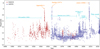 |
Fig. 1 Light curve of EX Lupi spanning the last ~130 yr. The photometry is a combination of Visible and V magnitudes taken from DASCH (red markers) and AAVSO (blue markers). It shows three large outbursts in 1944 (see Appendix A), 1955 (Herbig 1977) and 2008 (Jones 2008), multiple bursts reported by McLaughlin (1946), Bateson et al. (1991), Herbig et al. (2001), Herbig (2007) and the one presented in this work (see Fig. 2). |
2 EX Lupi
EX Lupi is the prototype of the EXor-type outbursts, and as such, it has been studied extensively by the astronomical community over the past decades. It is a young stellar object located at a distance of  (Gaia DR3; Gaia Collaboration 2016, 2023). Its photospheric lines indicate that it has a radial velocity (RV) period of 7.417 days (Kóspál et al. 2014). Alcalá et al. (2017) used an X-shooter spectrum to analyze EX Lupi, and among their results, they found an extinction AV = 1.1. Its first reported powerful (>5 mag) outburst began in 1955 (Herbig 1977) and was not observed spectroscopically. In 2008, EX Lupi underwent its largest outburst ever observed, during which the disk-to-star accretion rate increased to at least 2 × 10⁻⁷ M⊙ yr−1 (Juhász et al. 2012), leading to a more than 5 mag optical brightening. This elevated Ṁacc was confined to within the innermost 0.2–0.4au region (Goto et al. 2011; Kóspál et al. 2011). Indeed, the mass accretion in EX Lupi proceeds through remarkably stable accretion columns during both quiescence and outburst (Sicilia-Aguilar et al. 2012, 2015), and there are multiple indications for a complicated radial and azimuthal disk structure (e.g., Rigliaco et al. 2020). Observations during this powerful outburst provided the first evidence for on-going crystallization of silicate grains on the disk surface (Ábrahám et al. 2009), and follow-up observations showed evidence of vertical and radial mixing within the disk (Juhász et al. 2012; Ábrahám et al. 2019). Recent JWST/MIRI observations have shown that these crystals are now close to the water snowline, and as such, they are in a position to be incorporated into planetesimals (Kóspál et al. 2023). Moreover, the infrared molecular spectra showed strong signatures of enhanced UV photochemistry in the inner disk during outburst, with increased OH emission (probably from photo-dissociation of H2O) and the disappearance of organic molecules previously observed in quiescence (Banzatti et al. 2012). In addition to these extreme outbursts, EX Lupi has undergone at least 19 bursts in the past 130 yr (McLaughlin 1946; Bateson et al. 1991; Lehmann et al. 1995; Herbig et al. 2001; Herbig 2007; Ábrahám et al. 2019).
3 Observations
3.1 Optical and near-infrared photometry
We monitored EX Lupi at optical and near-infrared wavelengths between 2022 February 1 and 2022 September 6 with the Rapid Eye Mount (REM) telescope1 (LT 44025; PI: E. Fiorellino). We obtained images with an approximately nightly cadence using Sloan ɡ′r′i′z′and JHKs filters, except for several weeks in 2022 July through 2022 August when telescope operations had to be stopped due to an unusually strong and unprecedented snowstorm at La Silla. We obtained aperture photometry for the target and ten comparison stars within 3 of EX Lupi. We selected comparison stars with good quality APASS9 (Henden et al. 2015) and 2MASS (Cutri et al. 2003) photometry and with sufficiently constant brightness (σ V < 0.1 mag). We used an aperture radius of 3 pixels (or 3.67) and a sky annulus between 9 and 12 pixels (11″ and 22″). Data from the first few weeks of our monitoring were published in Kóspál et al. (2022), while the full data set is shown in Fig. 2.
Additional ɡ′r′i′z′ photometry of EX Lupi was obtained between 2022 March 30 and 2022 July 31 using the Las Cumbres Observatory global network of telescopes (LCOGT). Data sets were obtained with a roughly 5-h cadence but were sporadic due to weather and schedule constraints. The LCOGT utilizes the BANZAI pipeline2 (McCully et al. 2018) to perform standard image reduction, astrometric correction, and photometry. However, we found these pipeline results to be inconsistent, particularly for images with a low signal-to-noise ratio. Thus, we performed astrometric corrections on each frame using the Astrometry.net website3. Frames for which no solution could be found were discarded, except when an image was obtained within a set and the WCS information from a nearby corrected image could be used. We selected all sources in the frame cross-matched with the ATLAS-REFCAT 2 survey4 (Tonry et al. 2018) down to ɡ′~16mag. We pruned weak sources from each frame by carrying out aperture photometry, using a 20-pixel wide aperture and a background annulus between 30 and 40 pixels, and we discarded sources with a S/N less than five. Afterwards, we used least-squares to fit each source with a profile composed of a 2D Gaussian profile and a Moffat profile. The flux of each source was computed as the total integral of the best-fit profile, while we kept the uncertainty obtained with the aforementioned annulus. We then calculated a magnitude zero-point for each source using the flux estimated from our images and the magnitude from the ATLAS-REFCAT 2 catalog. Magnitude zero-points were converted to flux zero-points, 3σ outlying flux zero-points were discarded, and the average flux zero-point was then converted back to an average magnitude zero-point. This resulting value was then used to calculate a calibrated apparent magnitude for each source in the frame, including EX Lupi.
We complemented our photometric light curve with the ɡ-band measurements obtained as part of the All-Sky Automated Survey for Supernovae (ASAS-SN) project5, which monitors the full sky every night down to ɡ ~ 18 mag (Shappee et al. 2014; Kochanek et al. 2017). The earliest date with ASAS-SN data for EX Lupi in 2022 is January 14.
When we compared the magnitudes obtained with different facilities, we found that there are systematic differences. We corrected these by taking the median difference between the magnitudes of our REM program and the LCOGT and ASASSN data when we had observations on the same nights. In the case of the LCOGT data, the differences were +0.144 mag, +0.072 mag, +0.006 mag, and −0.200 mag for the ɡ′r′i′z′ filters, respectively, and for the ASAS-SN g photometry, we used a shift of +0.041 mag. We present the multi-filter light curve in Fig. 2, where these shifts have already been applied.
3.2 X-shooter spectroscopy
We obtained spectra of EX Lupi using the X-shooter échelle spectrograph (Vernet et al. 2011) on ESO’s Very Large Telescope (VLT) on 2022 March 27 (108.23N8.001, PI: F. Cruz-Sáenz de Miera) and 2022 July 29 (109.24F7.001, PI: F. Cruz-Sáenz de Miera). We complemented our spectroscopy data set with archival X-shooter observations taken on 2010 May 5 (085.C-0764, PI: H.M. Günther) and already published by Alcalá et al. (2017). We used the 0″.5, 0″.4, and 0″.4 wide slits, providing spectral resolutions of 9860, 18 300, and 11 400 in the UVB (0.30–0.56 µm), VIS (0.53–1.02 µm), and NIR (0.99–2.48 µm) arms, respectively. In the case of the two 2022 observations, we also observed EX Lupi with the 5” slit on the three arms to correct for slit losses and thus have a reliable flux calibration. The 2022 observations were carried out using an ABBA nodding pattern, while the 2010 ones were done with an AB pattern. We reduced the raw data using the X-shooter pipeline (v.3.5.3) within the EsoReflex environment, and we corrected for telluric absorption using ESO’s Molecfit (Kausch et al. 2015; Smette et al. 2015). The results of our calibration for the NIR arm of the 2010 snapshot had an abnormal continuum shape. Thus, for this arm, we used the calibrated product found in the ESO Science Archive6 and then corrected it for telluric absorption just as we did for our own data reduction. As final steps, we scaled each of the 2022 spectra so that their continuum levels matched those observed with the 5” broad slit. The 2010 observations did not include the broad slit as part of their setup; thus, we based our flux correction on a reprocessed version of the VJHK REM photometry published by Kóspál et al. (2014), which was coincidentally taken just 2 h before the X-shooter spectrum. These observations were reprocessed for the present study, which led to higher flux densities for the X-shooter spectrum by 20% in the UV and optical, while no change was observed in the infrared. We carried out synthetic photometry on the X-shooter spectrum and used the ratio between this and the observed photometry to find the scaling constants to correct the spectra. We utilized the V band to scale the UVB and VIS arms and the JHK bands to scale the NIR arm. In the case of the latter, we fit a straight line with the three ratios (and their respective wavelengths) to find the correction for the whole arm. We present the three X-shooter spectra in Fig. 3.
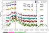 |
Fig. 2 Light curve of EX Lupi using optical and NIR photometry. Each color represents a different filter. Colors are indicated on the left side of the plot. The square, circle, and diamond symbols represent the different telescopes used to construct the light curve, and the “X” symbol indicates the synthetic photometry of the X-shooter spectra. The dates when these spectroscopic observations were taken are indicated with vertical dashed lines. The LCOGT and ASAS-SN magnitudes include the shifts mentioned in Sect. 3.1. The colored line beneath the light curve indicates the start and end dates of the different stages of the light curve. |
4 Results and analysis: Photometry
4.1 Light curve
In Fig. 2, we present the light curve for EX Lupi composed of different photometric filters at optical and near-infrared wavelengths. Using the ɡ band to monitor the brightness levels of EX Lupi, we divided the light curve into four stages: the “pre-burst” stage for all photometric points before 2022 February 14; the “brightening” stage for points between the previous date and when EX Lupi reached its burst peak on 2022 March 28; the “dimming” phase, which is immediately after EX Lupi reached the burst peak and finishes when it went back to its pre-burst brightness level of 2022 May 23; and finally the “post-burst” stage for all points after this latter date. The four stages are indicated in Fig. 2 beneath the light curves. We used these time intervals to determine the brightening and dimming rates, and we found that EX Lupi brightened and dimmed at 0.036 and 0.026 mag d−1, respectively.
 |
Fig. 3 Three X-shooter spectra: our two observations taken in 2022 and one archival epoch from 2010. The figure shows how significant the brightening of the whole spectrum due to the burst can be and how the spectrum had almost returned to its pre-burst shape after the burst ended. |
4.2 Period analysis
A visual inspection of our photometric light curve indicated that EX Lupi has periodic brightness fluctuations with a period similar to the rotational period of 7.417 days found by Kóspál et al. (2014). To determine the periodicity of EX Lupi in our data set, we produced Lomb-Scargle diagrams using only the ɡ-band photometry and its uncertainties, as it has the best time coverage due to a combination of ASAS-SN, REM, and LCOGT photometry. The other bands exhibit similar periodicity characteristics, albeit with lower significance (owing to their poor coverage), and are not considered in the rest of our periodicity analysis. Our first step was to remove the burst from the light curve, which we did by fitting four straight lines covering the four stages previously mentioned (pre-burst, brightening, dimming, and post-burst) and subtracting the best-fit lines from each phase. Afterwards, we produced a Lomb-Scargle diagram for each stage using the LombScargle function of Astropy (Astropy Collaboration 2013, 2018, 2022). The pre-burst stage consists only of 20 data points; thus, its Lomb-Scargle diagram did not produce significant results, and we did not analyze it further. The periodograms for the remaining three stages are shown in Fig. 4.
The dimming and post-outburst stages have periods of 7.4 days and are thus in agreement with the estimate by Kóspál et al. (2014) of 7.417 days within 0.5h. The periodogram of the brightening stage shows an almost flat peak, where the periods between 7.2 and 8.2 days have quite similar probabilities. An assumption of the Lomb-Scargle analysis is that the input light curve behaves sinusoidally. Therefore, a non-sinusoidal behavior of the light curve during this phase could broaden the width of this distribution.
It is not clear what physical process could have changed the behavior of the light curve for only this phase. However, we expect it to be related to changes in the accretion column, such as the appearance of a second accretion column at a different position on the star or the growth of the bright spot where the column makes contact with the star. Understanding the nature behind these changes is beyond the scope of this paper, and for now, we only conclude that the periodogram of the brightening phase should not be considered as a reliable deviation from the periodicity found by Kóspál et al. (2014).
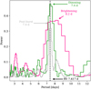 |
Fig. 4 Lomb-Scargle periodograms for three of the light curve stages. The periodograms show that the periods during the dimming and post-burst stages are in agreement with the estimate by Kóspál et al. (2014) from RV measurements. The periodogram of the brightening stage suggests that there was a change in the sinusoidal-like periodicity of EX Lupi. |
4.3 Color-color and color-magnitude diagrams
Our long-term multi-filter photometric monitoring can be used to construct color-magnitude and color-color diagrams, which can then be used to test whether the brightening of EX Lupi is caused by a decrease in the extinction or by an increase of the luminosity of the system. In Fig. 5, we present the color-magnitude diagrams using the seven photometric filters, and Fig. 6 shows the color-color diagram constructed with the three near-infrared filters. In both diagrams, the symbols are color-coded depending on the stage of the light curve as shown in the bottom of Fig. 2.
A visual comparison between our photometric data and the extinction vectors shows that, as reported by Kóspál et al. (2022), the burst did not follow the extinction vector. For a quick numerical check, we carried out a linear fit to each color-magnitude diagram and compared the fitted slope with the extinction vector from the extinction curve of Cardelli et al. (1989) with RV = 3.1. We found that, with the exception of the r – i color, nearly all colors follow a different path than the extinction, which suggests that the brightening was not due to a decrease in the line-of-sight extinction. In the g versus g – r diagram, a slight “knee” can be seen at ɡ ≈ 12.5 mag, and it is at this magnitude that EX Lupi was unequivocally in burst, while data points when EX Lupi was fainter than this magnitude mean that the source was in quiescence. The i – z color panel shows an interesting behavior where the brightening and the dimming stages follow different paths, with EX Lupi becoming slightly redder than when in quiescence while the dimming became bluer.
The near-infrared color-color diagram (Fig. 6) also shows how the colors of EX Lupi changed during the burst. The figure shows that an AV = 1.1 suggests that EX Lupi is a slightly extincted T Tauri star and, more importantly, that a change in extinction cannot explain the changes in the near-infrared colors seen during our monitoring of the burst. The changes in color during its 2022 burst are both significantly smaller and with a different direction than what has been observed in other EXortype sources during their (out)bursts, including EX Lupi itself during its powerful 2008 outburst (Lorenzetti et al. 2009, 2012). Indeed, while the other EXors shift to bluer J–H and Η–K colors, during its 2022 burst, EX Lupi became bluer in J – H and redder in H – K (see also the two rightmost panels of Fig. 5).
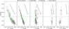 |
Fig. 5 Color-magnitude diagrams for the optical and NIR photometry. The circle and square symbols are the REM and LCOGT observations, respectively. The colors indicate the different stages of the light curve, where black is the pre-burst quiescence, pink is the brightening phase, green is the dimming phase, and gray is the post-burst quiescence (cf. Sect. 4.1). The arrow is the AV = 1.1 mag extinction vector following the extinction curve of Cardelli et al. (1989). The dotted horizontal lines indicate the ɡ = 12.5 mag threshold indicative of when EX Lupi is in burst. |
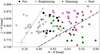 |
Fig. 6 Color-color diagram showing J – H versus H – K. The marker colors indicate the stages of the outburst as labeled in Fig. 5. The circle and “X” symbols are the REM photometry and the X-shooter synthetic photometry, respectively. The black tri markers indicate the colors when EX Lupi was in outburst (i.e., when ɡ ≤ 12.5 mag). In the bottom left, the light gray cross shows the median uncertainties of both photometric colors, and the arrow is the AV = 1.1 mag extinction vector following the extinction curve of Cardelli et al. (1989). The dash-dotted line is the locus of the unreddened Τ Tauri stars (Meyer et al. 1997). |
5 Results and analysis: Spectroscopy
The three spectra obtained for EX Lupi with X-shooter are presented in Fig. 3. During the peak of the burst, the level of the continuum is higher across the full wavelength coverage, and the overall shape of the spectrum is much flatter than for the two epochs in quiescence. The difference in flux levels between the two quiescent snapshots and the peak of the burst is, as expected, larger at shorter wavelengths, suggesting the appearance of an extra hot continuum during the burst. The Balmer jump is not seen in the burst spectrum, while it is clearly seen in the two quiescent spectra. Between the two quiescent measurements, the 2022 July spectrum has some UV excess with respect to the 2010 one. This excess can be interpreted as a slightly elevated Ṁacc leftover from the 2022 burst, as an intrinsic variability that occurs even during quiescence, or as changes related to the seven-day modulation found by Kóspál et al. (2014).
EX Lupi is an МО-type star; thus its spectra feature several photospheric absorption lines (Herbig et al. 2001). We removed the photospheric contribution from our three X-shooter spectra by using archival observations with the same instrument of an M0 pre-main sequence (or Class III) template star, TYC 7760-283-1 (085.C-0238, PI: J.M. Alcalá). To do this subtraction, we carried out an iterative fitting of the stellar template to the RV and veiling of EX Lupi. We split our continuum-normalized spectra into 5 nm chunks and varied these two parameters until we minimized the difference between our target and the template star. The best fits of some spectral chunks resulted in radial velocities that were significantly different from the median. Thus we shifted the complete photospheric spectrum to the median RV of each epoch and fit only the veiling for each spectral chunk. Finally, we subtracted the absorption component of our best-fitting template spectra from our EX Lupi measurements.
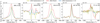 |
Fig. 7 Continuum-subtracted spectra of five emission lines found in the three epochs of EX Lupi observations that we used to calculate the Lacc. For better visual comparison between epochs, the 2010 and 2022 spectra have been scaled up by factors of 25 and 20, respectively. Below the name of each line is the rest wavelength for each transition, with the exception of the О I triplet where the wavelength is in between the three transitions. The yellow, red, and blue lines represent the 2010 quiescent, 2022 bursting, and 2022 post-burst quiescent spectra taken with X-shooter. The x-axes are the heliocentric-corrected velocities calculated with respect to the rest wavelength, and the vertical dashed line indicates the zero velocity. A visual inspection of these spectral lines shows how the burst strengthened and broadened the lines and, in the case of the О I triplet, how the blending worsened as a result of this. |
5.1 Emission lines
As previous works have shown, the EX Lupi spectrum (Fig. 3) is crowded with lines (Herbig et al. 2001; Herbig 2007; Kóspál et al. 2011; Sicilia-Aguilar et al. 2012; Alcalá et al. 2017; Rigliaco et al. 2020; Campbell-White et al. 2021). Similar to these previous studies, our observations show that the EX Lupi spectrum has multiple hydrogen emission lines of the Brackett, Balmer, and Paschen series. In addition, it exhibits multiple emission lines of neutral atoms (e.g., Na, Ca, Fe, Ti, К, Ni, Mn, Cr, Co, and V) and of ionized species (e.g., Ti, Sc, He, Ca, Cr, Fe). We used the National Institute of Standards and Technology (NIST) Atomic Spectra Database7 to identify the emission lines found for each of these atoms; however, an in-depth presentation of the lines will be prepared for a follow-up publication. Unsurprisingly, the spectrum taken close to the peak of the burst shows the largest number of lines, which are also stronger and broader than the pre- and post-burst spectra. In Fig. 7, we show a few of the lines we identified. A comparison between the three epochs is discussed in Sect. 6.1.
5.2 Accretion luminosity
Our first method to calculate the Lacc and Ṁacc is by using the empirical relationships between line luminosity and accretion luminosity as determined by Alcalá et al. (2017) for 38 emission lines that include several transitions for the Balmer, Paschen, and Brackett hydrogen series, plus some He I, He II, Ca II, Na I, and О I lines. For the first step of this process, we corrected the three photosphere-subtracted spectra for interstellar extinction using the extinction curve of Cardelli et al. (1989) with RV = 3.1 and assuming AV = 1.1 mag, as estimated by Alcalá et al. (2017). Next, we generated a sub-spectrum per accretion tracer using +2000 km s−1 as limits for each window. We estimated the continuum of each spectral window by fitting a straight line to the two-sigma clipped spectral window. After subtracting the continuum, we computed the line flux (Fline) by integrating all the emission inside a narrow spectral window tailored for each line. Finally, we used this line flux to calculate the line luminosity as Lline = 4πd2Fline and the accretion luminosity as log Lacc = a log Lline + b, where d is the distance to the source and a and b are parameters empirically obtained by Alcalá et al. (2017). In Fig. 7, we show five of the lines we used for this computation. In Table 1, we present our values of Lacc and Ṁacc for each line in each epoch, and in Tables B.1–B.3, we present the line fluxes and line luminosities. As mentioned earlier, our main goal is to study how the Lacc and Ṁacc have changed during the outburst; therefore, we only included the uncertainties of the line fluxes and of the a and b coefficients from Alcalá et al. (2017) because considering the uncertainties of the distance would only increase the size of the error bars without providing information for our analysis. Nevertheless, a comparison of EX Lupi with other young stars should take it into account.
For the second method, we fit slab models to the shorter wavelengths of the spectra (<1010 nm) without subtracting the photosphere and without correcting for extinction. The method is described in Manara et al. (2013) and has been used in studies of accretion in young stellar objects (e.g., Manara et al. 2016; Alcalá et al. 2017; Claes et al. 2022). It consists of finding the best χ2 fit between the observed spectrum and the sum of a photospheric template and a slab model, both reddened with an extinction AV. The slab model represents the excess emission due to accretion. The best-fit model is then used to estimate the accretion luminosity, Lacc.
We ran the fitting procedure for our three X-shooter spectra with a fixed spectral type (M0) and extinction (AV = 1.1). The 2010 spectrum has been fit by Alcalá et al. (2017) using the slab model, and we re-ran this analysis due to the difference in the slit-loss correction (see Sect. 3.2) and the fixed parameters. The fitting procedure also uses the previously mentioned distance to the object to scale the flux. In Fig. 8, we show a visual representation of our best-fitting results, where we show the observed spectra, the photospheric template, the emission of the accretion slab, and the total model for the three epochs. Using the bestfit values, we calculated Lacc values of 0.162 L⊙, 1.48 L⊙, and 0.292 L⊙ for the 2010 May, 2022 March, and 2022 July epochs, respectively.
In Fig. 9, we show a comparison of the Lacc calculated from each line per epoch with the two different methods. A comparison between these is discussed in Sect. 6.3.
Accretion luminosities (Lacc) and mass accretion rates (Ṁacc) for the three X-shooter epochs.
5.3 Mass accretion rate
We calculated the mass accretion rate taking the Lacc calculated for each emission line and from the slab modeling, and we used it as input for the relationship between Lacc and Ṁacc during magnetospheric accretion (Gullbring et al. 1998):
 (1)
(1)
where G is the gravitational constant; R⋆ and M⋆ are the stellar radius and mass, respectively; and Rin is the inner disk radius, for which we have assumed Rin = 5 R⋆ (Hartmann et al. 2016). For the two latter parameters, we first used the values determined by Sipos et al. (2009): R⋆ = 1.6R⊙ and M⋆ = 0.6 Μ⊙. Our resulting Ṁacc values are shown in Table 1.
The slab fitting procedure finds the best fit for the stellar luminosity per spectrum from which a stellar radius is calculated. It also finds a stellar mass by interpolating the best-fit stellar luminosity and effective temperature on different stellar tracks for young objects; see Manara et al. (2013) for details. This results in each epoch having a slightly different stellar radius and mass and each epoch being different from the ones calculated by Sipos et al. (2009). Using the Baraffe et al. (2015) tracks, we obtained Ṁасс values of 2.34 × 10⁻⁸ Μ⊙ yr−1, 1.62 × 10⁻⁷ М⊙уr−1, and 3.58 × 10⁻⁸ M⊙yr−1 for the 2010 May, 2022 March, and 2022 July epochs, respectively. Alternatively, the values obtained by using the Siess et al. (2000) tracks are 2.22 × 10⁻⁸М⊙уr−1, 1.57 × 10⁻⁷М⊙уr−1, and 3.41 × 10⁻⁸М⊙уr−1, respectively. We can only directly compare our results from both methods if we use the same stellar parameters. Thus, by taking the stellar parameters from Sipos et al. (2009), we found Ṁасс values of 1.72 × 10⁻⁸M⊙yr−1, 1.57 × 10⁻⁷М⊙уr−1, and 3.10 × 10⁻⁷М⊙уr−1 for the 2010 May, 2022 March, and 2022 July epochs, respectively. In the next section, we compare these values with the ones obtained using the emission lines.
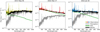 |
Fig. 8 Best-fitting slab models for the three epochs. Each panel contains the dereddened spectrum (each epoch represented by a different color), the photosphere template (gray), the best-fit slab (green), and the total combination of the slab and photosphere (black) used to calculate the χ2 during the fitting process. |
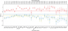 |
Fig. 9 Accretion luminosity (Lacc) calculated for each line per epoch. Each epoch is represented by a different color as shown earlier: yellow for the 2010 May 4 epoch, red for 2022 March 27, and blue for 2022 July 29. The horizontal lines are the values obtained from the slab model fitting per epoch. |
5.4 Evolution of the mass accretion rate during the outburst
The previous two analyses provided estimates of the Ṁacc at specific times, which is a strong constraint for our goals of learning how the Ṁacc evolved through the outburst and what the total mass accreted by EX Lupi was during this event. To follow the evolution of Ṁacc along the burst in a more detailed way, we decided to use the results from our slab modeling of the 2022 July 29 (i.e., post-burst) epoch as anchor to translate the light curves from the photometric monitoring into an “accretion curve”. The procedure is similar to that of the spectroscopic fitting, but instead of fitting to a spectrum, we calculated synthetic photometry of a large grid of models (i.e., the reddened sum of photosphere and slab) at the three optical filters (ɡ′r′i′) and then found the best-fitting model from the grid for each photometric epoch. The slabs are defined with three free parameters: different Tslab, ne, and τ. This procedure has fewer points to carry out the fitting; thus our results are degenerate, that is, slabs with different properties can fit the photometric points within the error bars. However, we found that the slab models that give the best match (lowest χ2) result in Lacc values within a relatively narrow range. Thus, while the parameters of the best-fitting models are degenerate, their Lacc values are not. We took these best-fitting Lacc estimates, averaged them to obtain an approximation of the Lacc per photometric epoch, and derived Ṁacc from them. We reran our calculations using the 2022 March 27 measurement (i.e., almost at the peak of the burst) as the anchor; however, the differences with respect to our chosen epoch are of less than 8%. Our resulting accretion curve is shown in Fig. 10, and we discuss its significance in the following section.
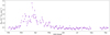 |
Fig. 10 Mass accretion rate as a function of time. The peak of the outburst reached a Ṁacc value seven times higher than the quiescent level, and the total mass integrated during the outburst was 2.9 × 10⁻⁸ M⊙, or 0.8 lunar masses. See Sect. 5.4 for more detail. |
6 Discussion
We have shown that the brightening experienced by EX Lupi in 2022 was caused by an increase in the mass accretion rate and not by a change in the line-of-sight extinction. EX Lupi has gone through more than a dozen bursts that have reached magnitudes brighter than V ~ 11 mag, such as the one presented in this work. Outbursts as powerful as the three previously experienced by EX Lupi have been shown to cause important changes in the mineralogy of the disk by the creation of silicate crystals (Ábrahám et al. 2009) and molecular abundances (Banzatti et al. 2012, 2015). Importantly, the impact that bursts can have on a system, either individually or collectively, is still understudied.
6.1 Line variability
In this subsection, we present a brief qualitative discussion of the features found in the emission lines of the three X-shooter spectra. A more detailed analysis of this is reserved for a future publication. In Fig. 7, we show a sub-set of continuum-subtracted emission lines that we use to showcase the differences and similarities between the three epochs. One of our snapshots was taken within a few days from the peak of the burst (red lines in Fig. 7), which is when we expect higher gas temperatures due to the increased accretion rate. Thus we expect this spectrum to show the largest differences with respect to the other two (blue and yellow lines in Fig. 7).
We found that during the peak of the burst, some lines become stronger and broader (e.g., Na I, O I, Hα), as expected from the analysis of the 2008 outburst of EX Lupi (Aspin et al. 2010; Goto et al. 2011; Kóspál et al. 2011; Sicilia-Aguilar et al. 2012, 2015; Banzatti et al. 2015). Some lines showed higher levels of asymmetry (e.g., Hα and Hβ), broad components reaching velocities in the order of a few 100 km s−1 (e.g., He I), and strong red-shifted absorption (e.g., O I triplet). As shown in the previous works, the blending between lines increased when EX Lupi was in burst. In the case of the O I triplet, we observed that during quiescence, the 777.4 and 777.5 nm lines are blended, while the 777.1 nm line is not, and while in burst, the three lines are blended with each other.
Our last snapshot was taken after EX Lupi went back to its pre-outburst levels of Ṁacc. Thus, we expected its spectrum to be similar to the one taken in 2010. However, we found that some lines have features that are in between the outburst and the quiescent spectra. For example, the Na I blue-shifted absorption has not returned to its pre-outburst shape in this snapshot, and its emission components remain broader. In the case of the O I triplet, the post-outburst emission lines are the same as the pre-outburst ones, but the red-shifted absorption feature seen during outburst can still be seen, albeit weaker. These differences indicate that even though the Ṁacc has gone back to normal, the physical properties (i.e., temperature and density) of the gas have not entirely done so. Therefore, any evolution caused by these outburst-driven changes could still be occurring months after the outburst ended.
Finally, we point out that the variations mentioned here should be taken with caution because the spectral lines of EX Lupi have shown variations that are not related to the accretion outburst (Sicilia-Aguilar et al. 2012, 2015; Campbell-White et al. 2021). Thus, we expect that the differences discussed here are caused by both the accretion burst and the rotational effects.
6.2 Searching for winds and jets with [O I]
The [O I] line at 630 nm is often used to study outflows, including those emanating from young T Tauri stars. There is a correlation between the kinematic properties obtained from analyzing the line and the Ṁacc of their ejecting stars (e.g., Nisini et al. 2018; Banzatti et al. 2019; Gangi et al. 2020, 2022). Since our spectral data set covers this line and we know that there was a temporary increase in the accretion, the 2022 burst of EX Lupi provides a great opportunity to study how the line changed due to the variations in the Ṁacc. In this paper, we present a short qualitative description of these changes as a more in-depth analysis is being prepared for a follow-up publication.
We extracted a narrow spectral window from the spectrum of each epoch, which we show in Fig. 11 plotted with respect to the heliocentric-corrected velocities. In the case of moderate-resolution spectra of T Tauri stars, the line profile of [O I] is often separated into two components: one with a low velocity (i.e., within a few kilometers per second from the systemic velocity of the star) and one with a high velocity (≥40 km s−1 away from the systemic). Therefore, we fit each spectral window using two Gaussian functions. The best fits are also shown in Fig. 11. The 2010 spectrum shows a strong feature in emission at ~130 km s−1, but we do not consider this as a real redshifted [O I] emission, and we do not take it into consideration in this discussion. Banzatti et al. (2019) carried out a study dedicated to this line using high spectral resolution near-infrared spectra of 64 T Tauri stars. Their sample included two spectra of EX Lupi, one taken during its 2008 outburst and another in its post-outburst stage in 2012, and they fit multiple Gaussian functions to each spectrum. In the bottom-right panel of Fig. 11, we show our best-fit Gaussians as well as the two from Banzatti et al. (2019).
The best fit of the 2010 spectrum is composed of two blueshifted broad components. The one with the highest velocity (−115 km s−1) has a comparable shape to the one found by Banzatti et al. (2019) in the 2012 spectrum, but we did not recover the narrower low-velocity component seen by them. During the 2022 burst, [O I] is only characterized by a broad low-velocity component. Indeed, fitting a single Gaussian produced an equally good result. Finally, the best fit found for the post-burst spectrum is composed of two low-velocity components, one broad and one narrow. The centroid velocities for all the low-velocity components are comparable with the spectral resolution of our observations, and thus, it is not clear whether they are blueshifted or redshifted.
The high-velocity component is used as a tracer of highvelocity jet emission, and the low-velocity is used as a tracer of slow winds. Therefore, the 2008 outburst (dark gray shaded area in Fig. 11) generated strong blueshifted and redshifted jet emission and strong blueshifted slow winds. By 2010 (yellow line) and 2012 (light gray area), the redshifted emission is not seen, but there is some remaining emission from the blueshifted jet. It is unclear if the lack of slow wind in the 2010 spectrum is real or a side effect of the low spectral resolution of X-shooter. During the 2022 burst (red line), there appears to be weak emission from slow winds, and by the time of the post-burst spectrum (blue line), the emission from this slow wind had strengthened. Banzatti et al. (2019) found that sources with higher Lacc have narrower low-velocity components. Thus, it is possible that the low spectral resolution diluted a narrow component that broadened as the Lacc decreased, making it detectable.
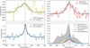 |
Fig. 11 Evolution of the [O I] line due to the 2022 burst and a comparison with the line profiles seen during and after the 2008 outburst. The top panels and the bottom-left panel show the [O I] line profile from the three X-shooter spectra analyzed in this work as a colored line and the best-fit Gaussians with a black line. In the bottom-right panel, we use colored lines to show the best-fit Gaussians and shaded-gray areas to show the best-fit Gaussians by Banzatti et al. (2019) calculated on their high-resolution spectra taken during the 2008 outburst and in quiescence in 2012. |
6.3 Accretion luminosity calculation
Using the emission lines, we found that for each epoch, the values of Lacc per emission line are in agreement with each other within a factor of a few when considering the uncertainties. In addition, we found that the pre- and post-outburst spectra resulted in the same values of Lacc, indicating that the outburst indeed had finished by late 2022 July. The outburst spectrum resulted in Lacc values higher than the 2010 and 2022 post-outburst spectra by factors of 11-380 and 9-250 (depending on the line), respectively. Based on the results of our slab modeling, the LACC increased by factors of five and nine when compared to the 2010 and 2022 quiescent spectra, respectively. The resulting values of Lacc can be found in Table 1, and we present a visual comparison of the Lacc values calculated with both methods in Fig. 9. For the quiescent spectra, most of the emission lines indicated lower values of Lacc than the slab model, and only a few lines are in agreement with the slab model within an factor of 2σ. For the outburst spectrum, more lines are in agreement with the slab model.
What causes the discrepancy between the two methods is not clear. We would naively expect that the coefficients found by Alcalá et al. (2017) would apply for EX Lupi, even when in outburst, for multiple reasons. First, the sample analyzed to find these relationships consisted of multiple T Tauri stars, including EX Lupi itself. Second, the stars in their sample were considered to be in quiescence, but even if they were experiencing EXor-type outbursts, the stars would be still experiencing magnetospheric accretion albeit at a higher rate (Sicilia-Aguilar et al. 2015). Third, the coefficients are the best-fit parameters of a linear fit found between the logarithm of the line luminosity (for each emission line) and the logarithm of the accretion luminosity, which was determined using the same slab model fitting procedure we used. Fourth, the line luminosities derived from our spectra are well within the range used by Alcalá et al. (2017) to determine these coefficients (see their Figs. E.1–E.6). Therefore, we suspect that these differences can be attributed to the computation of the line fluxes because this is highly sensitive to how the continuum-subtracted spectrum was constructed and what spectral range was used for each line. Indeed, EX Lupi has a high Ṁacc, even when in quiescence, thus finding its continuum level is not trivial for shorter wavelengths, and it is a line-rich star, which causes the accretion-tracing emission lines to be contaminated by other non-related lines. In addition, as mentioned earlier, when the star was in outburst, the line-blending is of higher concern because the lines became broader, and any lines that were previously too weak to be detected became stronger and possibly contaminated the accretion-tracing lines. These complications motivated us to only use the results from the slab modeling for the remainder of the discussion.
6.4 Mass accretion rate
The transformation of Lacc to Ṁacc depends on the assumptions of stellar radius and mass. For this discussion, we focus on the Ṁacc values calculated using the stellar parameters by Sipos et al. (2009). The accretion and stellar values used can be found in Table 1. Afterwards, we briefly discuss how our conclusions would change if we had chosen slightly different values for the stellar properties.
Our estimations of Ṁacc during quiescence are two orders of magnitude higher than was estimated previously by Sipos et al. (2009) and Sicilia-Aguilar et al. (2012). Both studies used the relationship between 10% width of Hα and the Ṁacc as determined by Natta et al. (2004) and obtained values on the order of 10−10 M⊙ yr−1. We verified that the discrepancies between their estimates and ours are not due to observational differences (e.g., signal-to-noise ratio and spectral resolution) by using the Natta et al. (2004) relationship with our Hα line profile. The 10% widths for our three Hα measurements are 320, 470, and 360 km s−1 for the 2010 May, 2022 March, and 2022 July epochs, respectively, which would indicate Ṁacc values of 1.6 × 10⁻¹⁰ M⊙ yr−1,4.6 × 10−9 M⊙ yr−1, and 3.8 × 10⁻¹⁰ M⊙ yr−1, respectively. Therefore, we confirm that using the 10% width of Hα on EX Lupi would underestimate the Ṁacc. Sipos et al. (2009) also calculated Lacc and Ṁacc based on the Paß line luminosity via the relationship by Muzerolle et al. (1998), and they found a value similar to the one from the Hα method. The Lacc calculated by Sipos et al. (2009) using Paß is an order of magnitude lower than our lowest Lacc estimate from the emission lines and two orders lower than our estimate using the slab model (see Table 1). These differences indicate that, when possible, one should aim to obtain more than one or two lines to determine the Ṁacc. When this is not possible, the estimated Ṁacc should be considered highly uncertain.
Our value of Lacc is in agreement with the value estimated by Alcalá et al. (2017), which is expected, as both estimates were done using the same spectra and with the only difference being the slit-loss correcting factor. However, the Ṁacc values are in disagreement by a factor of a few, but this can be explained by the differences in distance to EX Lupi and the stellar properties assumed during this calculation. These earlier estimates of Ṁacc, including the 10% widths of Hα, had suggested that EX Lupi is a young star with one of the lowest mass accretion rates. However, our Ṁacc results place EX Lupi as one of the strongest accretors, even when in quiescence (e.g., Alcalá et al. 2017; Banzatti et al. 2019).
We used our new estimate of the quiescent Ṁacc to determine how strong the 2008 outburst was. For that event, Juhász et al. (2012) determined an outbursting Ṁacc value of 2 × 10⁻⁷ M⊙ yr−1 using a Brγ measurement taken ~83days after the outburst reached its peak. However, their spectrum was taken when EX Lupi had dimmed by ~2 magnitudes (see their Fig. 1), and they assumed an extinction AV of 0 mag, so we considered their value of Ṁacc as a lower limit. Indeed, their estimate of Ṁacc for the 2008 outburst is comparable to our estimates for the 2022 burst. We obtained a new estimate using the methodology explained in Sect. 5.4 and anchoring our best-fit slab models to the photometry reported by Juhász et al. (2012) in their Table 1. This resulted in Ṁacc ≈ (8.96 ± 1.28) × 10−7 M⊙ yr−1 for the 2008 outburst. Therefore, we find that this powerful event was due to an increase of the Ṁacc by a factor of 52 and 29 when compared to our 2010 and 2022 quiescent spectra, respectively. These ratios are comparable to what has been found for other EXor type stars (e.g., Sicilia-Aguilar et al. 2017; Giannini et al. 2020).
As can be seen in Fig. 10, during the peak of its 2022 burst, EX Lupi reached Ṁacc values seven times higher than its quiescent level. As we have shown, the 2022 burst was weaker and shorter than the 2008 outburst by a factor of a few, which is similar to the factor of two found by Sicilia-Aguilar et al. (2017) between the outburst and burst of ASASSN-13db.
Our analysis has a couple of caveats to be considered when comparing our results to those from other works. First, we assumed that the extinction is AV = 1.1, when some studies have shown that this value could be as low as 0.0 (Sipos et al. 2009) or 0.1 (Wang et al. 2023), so our Ṁacc could be overestimated. We tested for this possible overestimation by running our slab model fitting routine, fixing AV = 0, and we found that the Ṁacc of all three epochs decreased by a factor of four to five. Therefore, our estimations of how Ṁacc increased from quiescence are consistent, but the impact of our choice of AV should be acknowledged when comparing our Ṁacc values with those calculated for other stars. The second caveat concerns our choice of stellar parameters and distance. The choice of these parameters can affect the value of Ṁacc by a factor of a few, as shown by our slab model fitting results in Sect. 5.3. Thus, when comparing our values with other analyses of EX Lupi, these stellar parameters (radius and mass) and the distance to the star must be taken into account. However, even though bursts are weaker than outbursts, they occur more frequently and could also have a significant impact on the young star.
6.5 Significance of one burst compared to other ones
Based on both its duration and amplitude, the 2022 burst is similar to the previous bursts seen in EX Lupi. Therefore, we can calculate the mass accreted by this event and apply this estimate to similar outbursts to obtain a rough estimate of the mass that has been accreted from the circumstellar disk during the outbursts. For the discussion in this section, we assumed that the disk of EX Lupi has a total mass of 0.01 M⊙ (Hales et al. 2018; White et al. 2020).
We calculated the total mass accreted during the 2022 burst by integrating the accretion curve found in Fig. 10. Between 2022 February 14 and 2022 May 28, EX Lupi accreted 2.90 × 10⁻⁸ M⊙ (0.8 lunar masses). To estimate how much more mass it accreted due to the burst, we took the quiescent Ṁacc value and multiplied it by the length of the burst (103 days), resulting in 1.14 × 10⁻⁸ M⊙ (0.3 lunar masses). Conversely, the excess mass accreted due to the burst was Mb = 1.76 × 10⁻⁸ M⊙ (0.5 lunar masses). Therefore, during the burst, EX Lupi accreted more than twice the mass it would have during quiescence, thus suggesting that a young star that experiences multiple bursts will deplete its circumstellar material faster than a non-outbursting one.
As mentioned above, finding the Ṁacc history during the 2008 outburst is not an easy task, and thus, estimating the total mass accreted during this event is highly uncertain. Our two estimates from Sect. 6.4 are uncertain, so we consider that the 2008 outburst reached a Ṁacc value 40 times higher than the quiescent level, and thus, that it accreted MB = 4.4 × 10⁻⁷ M⊙ = 0.15 M⊕= 11.9 Moon masses in total.
Over the past 30 yr, EX Lupi has gone through ten bursts and the powerful 2008 outburst. If we assume the ten bursts accreted a similar amount of mass as the 2022 burst, then the total mass accreted during the past three decades is (Mq × 30) + (Mb × 10) + MB = 1.8 × 10⁻⁶ M⊙. This indicates that the outbursts were responsible for 34% of the total mass accreted in the considered time span, of which 10 and 24% were the product of the bursts and the outburst, respectively. If we consider that EX Lupi lacks an envelope to replenish the disk material (Sipos et al. 2009) and assume that the accretion in EX Lupi will remain as active as it has been for these last three decades, it will deplete the total disk mass in 160 000 yr.
Nonetheless, we know from our full light curve (Fig. 1) that when compared with the 130 yr of data, the accretion in EX Lupi has been particularly active in these last three decades. The pre 1990 data of the light curve is not as high quality as the more recent measurements, so estimating the total mass accreted during this time is still more uncertain. Between 1950 and 1990, Bateson et al. (1991) reported several brightenings in the light curve, including the powerful 1955 outburst, and our inspection of the light curve indicates that during these decades, there were four bursts. The earlier data are harder to assess. We find that there were at least five bursts in the light curve of McLaughlin (1946) plus the 1944 powerful outburst that had not been reported previously. Our final tally of bursts and outbursts indicate that in the past 130 yr, there were at least 19 bursts and three outbursts, making the total accreted mass (Mq × 130) + (Mb × 19) + (MB × 3) = 6.9 × 10⁻⁶ M⊙. A similar behavior in the Ṁacc would consume the disk mass in 190 000 yr. Finally, if we assume that EX Lupi will not experience another burst or outburst and thus remain at its quiescent Ṁacc, it will deplete its mass reservoir in 250 000 yr.
As mentioned earlier, this estimate is uncertain due to the multiple assumptions, such as the constant quiescent Ṁacc (which might not be stable if we consider that the “quiescent” brightness of the full light curve has changed by ~1 magnitude between, e.g., 1980 and 2020) and the lower limit of detected bursts and outbursts (due to the long gaps in the photometric coverage). Still, all estimates suggest that EX Lupi is close to spending its disk mass and will soon move to its next evolutionary phase.
7 Summary and conclusions
The system EX Lupi started experiencing a new brightening event in 2022 February and by late May it had returned to its normal brightness levels. We carried out multi-filter photometric monitoring and obtained two spectroscopic measurements. We found that this brightening was the result of an increase in the mass accretion rate. Our main findings are as follows:
Using g-band photometry, we found that the burst started in the middle of 2022 February and ended in late 2022 May. EX Lupi brightened by ~2mag at its peak and experienced brightening and dimming rates of 0.036 mag day−1 and 0.026 mag day−1, respectively.
We saw some periodicity in the light curve and analyzed it using Lomb-Scargle diagrams at different stages of the burst. However, we did not find significant changes in the period of these brightness fluctuations. We find a ~7.4-day period in EX Lupi during and post outburst as well as during quiescence, consistent with previous studies.
Using color-color and color-magnitude diagrams, we found that the brightening was not caused by changes in the extinction.
The spectra of EX Lupi are crowded with lines due to neutral and ionized atoms, and these became broader and stronger during the burst. We briefly discussed the evolution of the [O I] line, which traces jets and winds, and found differences in the line profile that are tentatively due to the burst but can also be explained by the spectral resolution of our observations.
Using different emission lines to calculate the Lacc, we derived a wide range of values for each epoch, and these differ from the values calculated with the slab model. Using the emission lines leads to higher uncertainties, in particular with the calculation of the continuum, and we thus recommend using the slab model when possible or more than one emission line to calculate the Lacc.
Based on the slab model fitting, during the burst, the Ṁacc increased by a factor of approximately seven. The total mass accreted during the burst was 0.8 lunar masses, which is ~1.5 times more than what would have been accreted in the same length of time with the quiescent level of Ṁacc.
We have estimated that for the past 130 yr, 30% of the accreted mass has been the product of bursts and outbursts. Therefore, we find that these events can significantly accelerate the evolution of a young stellar object.
The combination of the mass of the disk surrounding EX Lupi and an extrapolation of the accretion history based on 130 yr of observations suggests that in the absence of significant replenishment, the disk will be depleted in a few hundred thousand years, and thus, it is close to reaching its next evolutionary stage.
The 2022 burst of EX Lupi provided great insight into the short-term changes brought by a single accretion burst and shed some light onto the long-term effects that multiple bursts and outbursts can have on a young star. However, several questions remain regarding the accretion bursts and outbursts (Fischer et al. 2023). In-depth multi-wavelength observational studies of future bursts and outbursts are needed to begin answering these remaining questions.
Acknowledgements
This project has received funding from the European Research Council (ERC) under the European Union’s Horizon 2020 research and innovation programme under grant agreement No 716155 (SACCRED). Funded by the European Union (ERC, WANDA, 101039452). Views and opinions expressed are however those of the author(s) only and do not necessarily reflect those of the European Union or the European Research Council Executive Agency. Neither the European Union nor the granting authority can be held responsible for them. INAF co-authors acknowledge the support of PRIN-INAF 2019 “Spectroscopically Tracing the Disk Dispersal Evolution (STRADE)” and by the Large Grant INAF 2022 YODA (YSOs Outflows, Disks and Accretion: towards a global framework for the evolution of planet forming systems) Zs.M.Sz. acknowledges funding from a St Leonards scholarship from the University of St Andrews. Zs.M.Sz. is a member of the International Max Planck Research School (IMPRS) for Astronomy and Astrophysics at the Universities of Bonn and Cologne. Zs.N. was supported by the János Bolyai Research Scholarship of the Hungarian Academy of Sciences. We acknowledge support from the ESA PRODEX contract nr. 4000132054. We thank the REM staff for the observational support. This work makes use of observations from the Las Cumbres Observatory global telescope network. Based on observations collected at the European Southern Observatory under ESO programmes 085.C-0764(A), 108.23N8.001, and 109.24F7.001.
Appendix A The 1944 outburst of EX Lupi
We searched for EX Lupi photometry on the Digital Access to a Sky Century at Harvard (DASCH) project website.8 Their light curve tool offers four different options for the input catalog to be used as reference for the magnitude estimation. We selected the APASS Input Catalog, which offers Visible magnitudes and does not need a correction factor with respect to the values obtained from AAVSO. The full light curve can be seen in Fig. 1. It roughly covers the periods from 1893 to 1953, 1970 to 1973, and 1978 to 1989; The earliest plate is from 1893 June 24.
In Fig. A.1, we show the three known powerful outbursts of EX Lupi. The sampling of the light curve for the three events is different. We lack the data points to know when the 1944 outburst began and when the star returned to quiescence. The 1955 outburst is the best sampled event, with adequate coverage of the brightening and dimming phases, and the 2008 outburst has a few data points still in brightening, but we lack information of when EX Lupi started to brighten. Nevertheless, we have shifted the three events to approximately align them by assuming that the first data point of the 1944 event is from just after the outburst reached its peak. The MJD Day 0 are 31400, 35250, and 54410 for the 1944, 1955, and 2008 outbursts, respectively.
The three outbursts show significant variability in their bright stages, dimming by as much as 2~3 mag. The 1955 outburst was the shortest, lasting for ~250 days. If we assume that EX Lupi reached its maximum brightness on the first day for which we have data of the 1944 outburst (day ~100 in Fig. A.1), then this event is the longest outburst yet, lasting ≳330 days. The three outbursts reached comparable magnitudes in their heightened stages, which is indicative of similar physical conditions for each outburst. However, there is spectroscopy only for the 2008 event, and it is of moderate quality. Therefore, the determination of these physical properties shall be pursued in a future powerful outburst.
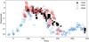 |
Fig. A.1 The three known powerful outbursts of EX Lupi. The events have been shifted to approximately align with the length of their outbursts. |
Appendix B Line fluxes and line luminosities
In this appendix, we present the line fluxes and line luminosities for each accretion-tracing emission line per epoch.
References
- Ábrahám, P., Juhász, A., Dullemond, C. P., et al. 2009, Nature, 459, 224 [Google Scholar]
- Ábrahám, P., Chen, L., Kóspál, Á., et al. 2019, ApJ, 887, 156 [Google Scholar]
- Alcalá, J. M., Manara, C. F., Natta, A., et al. 2017, A&A, 600, A20 [NASA ADS] [CrossRef] [EDP Sciences] [Google Scholar]
- Aspin, C., Reipurth, B., Herczeg, G. J., & Capak, P. 2010, ApJ, 719, L50 [NASA ADS] [CrossRef] [Google Scholar]
- Astropy Collaboration (Robitaille, T. P., et al.) 2013, A&A, 558, A33 [NASA ADS] [CrossRef] [EDP Sciences] [Google Scholar]
- Astropy Collaboration (Price-Whelan, A. M., et al.) 2018, AJ, 156, 123 [Google Scholar]
- Astropy Collaboration (Price-Whelan, A. M., et al.) 2022, ApJ, 935, 167 [NASA ADS] [CrossRef] [Google Scholar]
- Audard, M., Ábrahám, P., Dunham, M. M., et al. 2014, in Protostars and Planets VI, eds. H. Beuther, R. S. Klessen, C. P. Dullemond, & T. Henning (Tucson: University of Arizona Press), 387 [Google Scholar]
- Banzatti, A., Meyer, M. R., Bruderer, S., et al. 2012, ApJ, 745, 90 [NASA ADS] [CrossRef] [Google Scholar]
- Banzatti, A., Pontoppidan, K. M., Bruderer, S., Muzerolle, J., & Meyer, M. R. 2015, ApJ, 798, L16 [Google Scholar]
- Banzatti, A., Pascucci, I., Edwards, S., et al. 2019, ApJ, 870, 76 [Google Scholar]
- Baraffe, I., Homeier, D., Allard, F., & Chabrier, G. 2015, A&A, 577, A42 [NASA ADS] [CrossRef] [EDP Sciences] [Google Scholar]
- Bateson, F. M., McIntosh, R., & Brunt, D. 1991, Royal Astronomical Society of New Zealand Publications of Variable Star Section (New Zealand: Variable Star Section, Royal Astronomical Society of New Zealand), 16, 49 [NASA ADS] [Google Scholar]
- Campbell-White, J., Sicilia-Aguilar, A., Manara, C. F., et al. 2021, MNRAS, 507, 3331 [NASA ADS] [CrossRef] [Google Scholar]
- Cardelli, J. A., Clayton, G. C., & Mathis, J. S. 1989, ApJ, 345, 245 [Google Scholar]
- Claes, R. A. B., Manara, C. F., Garcia-Lopez, R., et al. 2022, A&A, 664, L7 [NASA ADS] [CrossRef] [EDP Sciences] [Google Scholar]
- Cruz-Sáenz de Miera, F., Kóspál, Á., Ábrahám, P., et al. 2022, ApJ, 927, 125 [CrossRef] [Google Scholar]
- Cutri, R. M., Skrutskie, M. F., van Dyk, S., et al. 2003, VizieR Online Data Catalog: II/246 [Google Scholar]
- Fischer, W. J., Hillenbrand, L. A., Herczeg, G. J., et al. 2023, ASP Conf. Ser., 534, 355 [NASA ADS] [Google Scholar]
- Gaia Collaboration (Prusti, T., et al.) 2016, A&A, 595, A1 [NASA ADS] [CrossRef] [EDP Sciences] [Google Scholar]
- Gaia Collaboration (Vallenari, A., et al.) 2023, A&A, 674, A1 [NASA ADS] [CrossRef] [EDP Sciences] [Google Scholar]
- Gangi, M., Nisini, B., Antoniucci, S., et al. 2020, A&A, 643, A32 [NASA ADS] [CrossRef] [EDP Sciences] [Google Scholar]
- Gangi, M., Antoniucci, S., Biazzo, K., et al. 2022, A&A, 667, A124 [NASA ADS] [CrossRef] [EDP Sciences] [Google Scholar]
- Ghosh, A., Sharma, S., Ninan, J. P., et al. 2022, ApJ, 926, 68 [NASA ADS] [CrossRef] [Google Scholar]
- Giannini, T., Giunta, A., Lorenzetti, D., et al. 2020, A&A, 637, A83 [NASA ADS] [CrossRef] [EDP Sciences] [Google Scholar]
- Goto, M., Regály, Z., Dullemond, C. P., et al. 2011, ApJ, 728, 5 [CrossRef] [Google Scholar]
- Gullbring, E., Hartmann, L., Briceño, C., & Calvet, N. 1998, ApJ, 492, 323 [Google Scholar]
- Hales, A. S., Pérez, S., Saito, M., et al. 2018, ApJ, 859, 111 [Google Scholar]
- Hartmann, L., & Kenyon, S. J. 1996, ARA&A, 34, 207 [NASA ADS] [CrossRef] [Google Scholar]
- Hartmann, L., Herczeg, G., & Calvet, N. 2016, ARA&A, 54, 135 [Google Scholar]
- Henden, A. A., Levine, S., Terrell, D., & Welch, D. L. 2015, AAS Meeting Abs., 225, 336.16 [Google Scholar]
- Herbig, G. H. 1977, ApJ, 217, 693 [NASA ADS] [CrossRef] [Google Scholar]
- Herbig, G. H. 1989, European Southern Observatory Conference and WorkshopProceedings, 33, 233 [NASA ADS] [Google Scholar]
- Herbig, G. H. 2007, AJ, 133, 2679 [NASA ADS] [CrossRef] [Google Scholar]
- Herbig, G. H., Aspin, C., Gilmore, A. C., Imhoff, C. L., & Jones, A. F. 2001, PASP, 113, 1547 [Google Scholar]
- Hillenbrand, L. A. 2019, ATel, 13321, 1 [NASA ADS] [Google Scholar]
- Jones, A. F. A. L. 2008, Central Bureau Electronic Telegrams, 1217, 1 [NASA ADS] [Google Scholar]
- Juhász, A., Dullemond, C. P., van Boekel, R., et al. 2012, ApJ, 744, 118 [Google Scholar]
- Kausch, W., Noll, S., Smette, A., et al. 2015, A&A, 576, A78 [NASA ADS] [CrossRef] [EDP Sciences] [Google Scholar]
- Kochanek, C. S., Shappee, B. J., Stanek, K. Z., et al. 2017, PASP, 129, 104502 [Google Scholar]
- Kóspál, Á., Ábrahám, P., Goto, M., et al. 2011, ApJ, 736, 72 [CrossRef] [Google Scholar]
- Kóspál, Á., Mohler-Fischer, M., Sicilia-Aguilar, A., et al. 2014, A&A, 561, A61 [NASA ADS] [CrossRef] [EDP Sciences] [Google Scholar]
- Kóspál, Á., Fiorellino, E., Ábrahám, P., Giannini, T., & Nisini, B. 2022, Res.Notes Am. Astron. Soc., 6, 52 [Google Scholar]
- Kóspál, Á., Ábrahám, P., Diehl, L., et al. 2023, ApJ, 945, L7 [CrossRef] [Google Scholar]
- Lehmann, T., Reipurth, B., & Brandner, W. 1995, A&A, 300, L9 [NASA ADS] [Google Scholar]
- Liu, H., Herczeg, G. J., Johnstone, D., et al. 2022, ApJ, 936, 152 [NASA ADS] [CrossRef] [Google Scholar]
- Lorenzetti, D., Larionov, V. M., Giannini, T., et al. 2009, ApJ, 693, 1056 [NASA ADS] [CrossRef] [Google Scholar]
- Lorenzetti, D., Antoniucci, S., Giannini, T., et al. 2012, ApJ, 749, 188 [NASA ADS] [CrossRef] [Google Scholar]
- Manara, C. F., Beccari, G., Da Rio, N., et al. 2013, A&A, 558, A114 [NASA ADS] [CrossRef] [EDP Sciences] [Google Scholar]
- Manara, C. F., Fedele, D., Herczeg, G. J., & Teixeira, P. S. 2016, A&A, 585, A136 [NASA ADS] [CrossRef] [EDP Sciences] [Google Scholar]
- Manara, C. F., Ansdell, M., Rosotti, G. P., et al. 2023, ASP Conf. Ser., 534, 539 [NASA ADS] [Google Scholar]
- McCully, C., Turner, M., Volgenau, N., et al. 2018, https://zenodo.org/record/1257560 [Google Scholar]
- McLaughlin, D. B. 1946, AJ, 52, 109 [CrossRef] [Google Scholar]
- Meyer, M. R., Calvet, N., & Hillenbrand, L. A. 1997, AJ, 114, 288 [Google Scholar]
- Muzerolle, J., Hartmann, L., & Calvet, N. 1998, AJ, 116, 2965 [NASA ADS] [CrossRef] [Google Scholar]
- Natta, A., Testi, L., Neri, R., Shepherd, D. S., & Wilner, D. J. 2004, A&A, 416, 179 [NASA ADS] [CrossRef] [EDP Sciences] [Google Scholar]
- Nisini, B., Antoniucci, S., Alcalá, J. M., et al. 2018, A&A, 609, A87 [EDP Sciences] [Google Scholar]
- Park, S., Kóspál, Á., Ábrahám, P., et al. 2022, ApJ, 941, 165 [NASA ADS] [CrossRef] [Google Scholar]
- Rigliaco, E., Gratton, R., Kóspál, Á., et al. 2020, A&A, 641, A33 [NASA ADS] [CrossRef] [EDP Sciences] [Google Scholar]
- Shappee, B. J., Prieto, J. L., Grupe, D., et al. 2014, ApJ, 788, 48 [Google Scholar]
- Sicilia-Aguilar, A., Kóspál, Á., Setiawan, J., et al. 2012, A&A, 544, A93 [NASA ADS] [CrossRef] [EDP Sciences] [Google Scholar]
- Sicilia-Aguilar, A., Fang, M., Roccatagliata, V., et al. 2015, A&A, 580, A82 [NASA ADS] [CrossRef] [EDP Sciences] [Google Scholar]
- Sicilia-Aguilar, A., Oprandi, A., Froebrich, D., et al. 2017, A&A, 607, A127 [NASA ADS] [CrossRef] [EDP Sciences] [Google Scholar]
- Sicilia-Aguilar, A., Campbell-White, J., Roccatagliata, V., et al. 2023, MNRAS, submitted [Google Scholar]
- Siess, L., Dufour, E., & Forestini, M. 2000, A&A, 358, 593 [Google Scholar]
- Sipos, N., Ábrahám, P., Acosta-Pulido, J., et al. 2009, A&A, 507, 881 [NASA ADS] [CrossRef] [EDP Sciences] [Google Scholar]
- Smette, A., Sana, H., Noll, S., et al. 2015, A&A, 576, A77 [NASA ADS] [CrossRef] [EDP Sciences] [Google Scholar]
- Tonry, J. L., Denneau, L., Flewelling, H., et al. 2018, ApJ, 867, 105 [NASA ADS] [CrossRef] [Google Scholar]
- Vernet, J., Dekker, H., D’Odorico, S., et al. 2011, A&A, 536, A105 [NASA ADS] [CrossRef] [EDP Sciences] [Google Scholar]
- Wang, M.-T., Herczeg, G. J., Liu, H.-G., et al. 2023, ApJ, submitted [arXiv:2308.11895] [Google Scholar]
- White, J. A., Kóspál, Á., Hughes, A. G., et al. 2020, ApJ, 904, 37 [CrossRef] [Google Scholar]
- Zhou, L., & Herczeg, G. J. 2022, ATel, 15271, 1 [NASA ADS] [Google Scholar]
REM is a 60 cm mirror diameter automatic telescope at La Silla (Chile) operated by the Italian National Institute for Astrophysics (INAF). http://www.rem.inaf.it/
All Tables
Accretion luminosities (Lacc) and mass accretion rates (Ṁacc) for the three X-shooter epochs.
All Figures
|
Fig. 1 Light curve of EX Lupi spanning the last ~130 yr. The photometry is a combination of Visible and V magnitudes taken from DASCH (red markers) and AAVSO (blue markers). It shows three large outbursts in 1944 (see Appendix A), 1955 (Herbig 1977) and 2008 (Jones 2008), multiple bursts reported by McLaughlin (1946), Bateson et al. (1991), Herbig et al. (2001), Herbig (2007) and the one presented in this work (see Fig. 2). |
| In the text | |
|
Fig. 2 Light curve of EX Lupi using optical and NIR photometry. Each color represents a different filter. Colors are indicated on the left side of the plot. The square, circle, and diamond symbols represent the different telescopes used to construct the light curve, and the “X” symbol indicates the synthetic photometry of the X-shooter spectra. The dates when these spectroscopic observations were taken are indicated with vertical dashed lines. The LCOGT and ASAS-SN magnitudes include the shifts mentioned in Sect. 3.1. The colored line beneath the light curve indicates the start and end dates of the different stages of the light curve. |
| In the text | |
|
Fig. 3 Three X-shooter spectra: our two observations taken in 2022 and one archival epoch from 2010. The figure shows how significant the brightening of the whole spectrum due to the burst can be and how the spectrum had almost returned to its pre-burst shape after the burst ended. |
| In the text | |
|
Fig. 4 Lomb-Scargle periodograms for three of the light curve stages. The periodograms show that the periods during the dimming and post-burst stages are in agreement with the estimate by Kóspál et al. (2014) from RV measurements. The periodogram of the brightening stage suggests that there was a change in the sinusoidal-like periodicity of EX Lupi. |
| In the text | |
|
Fig. 5 Color-magnitude diagrams for the optical and NIR photometry. The circle and square symbols are the REM and LCOGT observations, respectively. The colors indicate the different stages of the light curve, where black is the pre-burst quiescence, pink is the brightening phase, green is the dimming phase, and gray is the post-burst quiescence (cf. Sect. 4.1). The arrow is the AV = 1.1 mag extinction vector following the extinction curve of Cardelli et al. (1989). The dotted horizontal lines indicate the ɡ = 12.5 mag threshold indicative of when EX Lupi is in burst. |
| In the text | |
|
Fig. 6 Color-color diagram showing J – H versus H – K. The marker colors indicate the stages of the outburst as labeled in Fig. 5. The circle and “X” symbols are the REM photometry and the X-shooter synthetic photometry, respectively. The black tri markers indicate the colors when EX Lupi was in outburst (i.e., when ɡ ≤ 12.5 mag). In the bottom left, the light gray cross shows the median uncertainties of both photometric colors, and the arrow is the AV = 1.1 mag extinction vector following the extinction curve of Cardelli et al. (1989). The dash-dotted line is the locus of the unreddened Τ Tauri stars (Meyer et al. 1997). |
| In the text | |
|
Fig. 7 Continuum-subtracted spectra of five emission lines found in the three epochs of EX Lupi observations that we used to calculate the Lacc. For better visual comparison between epochs, the 2010 and 2022 spectra have been scaled up by factors of 25 and 20, respectively. Below the name of each line is the rest wavelength for each transition, with the exception of the О I triplet where the wavelength is in between the three transitions. The yellow, red, and blue lines represent the 2010 quiescent, 2022 bursting, and 2022 post-burst quiescent spectra taken with X-shooter. The x-axes are the heliocentric-corrected velocities calculated with respect to the rest wavelength, and the vertical dashed line indicates the zero velocity. A visual inspection of these spectral lines shows how the burst strengthened and broadened the lines and, in the case of the О I triplet, how the blending worsened as a result of this. |
| In the text | |
|
Fig. 8 Best-fitting slab models for the three epochs. Each panel contains the dereddened spectrum (each epoch represented by a different color), the photosphere template (gray), the best-fit slab (green), and the total combination of the slab and photosphere (black) used to calculate the χ2 during the fitting process. |
| In the text | |
|
Fig. 9 Accretion luminosity (Lacc) calculated for each line per epoch. Each epoch is represented by a different color as shown earlier: yellow for the 2010 May 4 epoch, red for 2022 March 27, and blue for 2022 July 29. The horizontal lines are the values obtained from the slab model fitting per epoch. |
| In the text | |
|
Fig. 10 Mass accretion rate as a function of time. The peak of the outburst reached a Ṁacc value seven times higher than the quiescent level, and the total mass integrated during the outburst was 2.9 × 10⁻⁸ M⊙, or 0.8 lunar masses. See Sect. 5.4 for more detail. |
| In the text | |
|
Fig. 11 Evolution of the [O I] line due to the 2022 burst and a comparison with the line profiles seen during and after the 2008 outburst. The top panels and the bottom-left panel show the [O I] line profile from the three X-shooter spectra analyzed in this work as a colored line and the best-fit Gaussians with a black line. In the bottom-right panel, we use colored lines to show the best-fit Gaussians and shaded-gray areas to show the best-fit Gaussians by Banzatti et al. (2019) calculated on their high-resolution spectra taken during the 2008 outburst and in quiescence in 2012. |
| In the text | |
|
Fig. A.1 The three known powerful outbursts of EX Lupi. The events have been shifted to approximately align with the length of their outbursts. |
| In the text | |
Current usage metrics show cumulative count of Article Views (full-text article views including HTML views, PDF and ePub downloads, according to the available data) and Abstracts Views on Vision4Press platform.
Data correspond to usage on the plateform after 2015. The current usage metrics is available 48-96 hours after online publication and is updated daily on week days.
Initial download of the metrics may take a while.