| Issue |
A&A
Volume 685, May 2024
|
|
|---|---|---|
| Article Number | A45 | |
| Number of page(s) | 15 | |
| Section | Astrophysical processes | |
| DOI | https://doi.org/10.1051/0004-6361/202348357 | |
| Published online | 03 May 2024 | |
Simulating the tidal disruption of stars by stellar-mass black holes using moving-mesh hydrodynamics
1
Max-Planck-Institut für Astrophysik, Karl-Schwarzschild-Straße 1, 85748 Garching bei München, Germany
e-mail: This email address is being protected from spambots. You need JavaScript enabled to view it.
2
Physics and Astronomy Department, Johns Hopkins University, Baltimore, MD 21218, USA
3
Anton Pannekoek Institute for Astronomy, University of Amsterdam, Science Park 904, 1098 XH Amsterdam, The Netherlands
4
Physics Department, Technion – Israel Institute of Technology, Haifa 3200003, Israel
Received:
23
October
2023
Accepted:
10
February
2024
Abstract
In the centers of dense star clusters, close encounters between stars and compact objects are likely to occur. We studied tidal disruption events of main-sequence (MS) stars by stellar-mass black holes (termed μTDEs), which can shed light on the processes occurring in these clusters, including being an avenue in the mass growth of stellar-mass BHs. Using the moving-mesh hydrodynamics code AREPO, we performed a suite of 58 hydrodynamics simulations of partial μTDEs of realistic, MESA-generated MS stars by varying the initial mass of the star (0.5 M⊙ and 1 M⊙), the age of the star (zero-age, middle-age and terminal-age), the mass of the black hole (10 M⊙ and 40 M⊙), and the impact parameter (yielding almost no mass loss to full disruption). We then examined the dependence of the masses, spins, and orbital parameters of the partially disrupted remnant on the initial encounter parameters. We find that the mass lost from a star decreases roughly exponentially with increasing approach distance and that a 1 M⊙ star loses less mass than a 0.5 M⊙ one. Moreover, a more evolved star is less susceptible to mass loss. Tidal torques at the closest approach spin up the remnant very close to break-up velocity when the impact parameter is low. The remnant star can be bound (eccentric) or unbound (hyperbolic) to the black hole; hyperbolic orbits occur when the star’s central density concentration is relatively low and the black-hole-star mass ratio is high, which is the case for the disruption of a 0.5 M⊙ star. Finally, we provide best-fit analytical formulae for the aforementioned range of parameters that can be incorporated into cluster codes to model star-black-hole interaction more accurately.
Key words: black hole physics / gravitation / hydrodynamics / stars: kinematics and dynamics
© The Authors 2024
 Open Access article, published by EDP Sciences, under the terms of the Creative Commons Attribution License (https://creativecommons.org/licenses/by/4.0), which permits unrestricted use, distribution, and reproduction in any medium, provided the original work is properly cited.
This article is published in open access under the Subscribe to Open model.
Open access funding provided by Max Planck Society.
1. Introduction
Tidal disruption events (TDEs) of stars by supermassive black holes (SMBHs) have been a subject of significant interest in the past decade (see Stone et al. 2019; Gezari 2021 for reviews). TDEs by SMBHs are observed as transients in multiple wavelengths (Gezari 2021), with ∼100 such events having been detected by observatories in the optical (ASAS-SN: Kochanek et al. 2017, ZTF: Bellm et al. 2019, PTF: Law et al. 2009, PS: Chambers et al. 2016, ATLAS: Tonry et al. 2018, SDSS: Kollmeier et al. 2019, OGLE: Udalski et al. 2015), X-ray (ROSAT: Voges et al. 1999, Swift: Gehrels et al. 2004, XMM: Jansen et al. 2001, Chandra: Weisskopf et al. 2000), and UV (GALEX: Martin et al. 2005).
In this work, we examine TDEs of stars by stellar-mass black holes or SBHs (termed μTDEs). These are less studied and have only garnered interest recently. Although μTDEs have lower observable rates (Perets et al. 2016), they can shed light on the processes occurring in the centers of globular and nuclear star clusters where they are most likely to occur. In particular, they are an important avenue in the mass growth of SBHs to form intermediate-mass black holes (IMBHs, e.g., Stone et al. 2017; Rizzuto et al. 2023). However, these studies make simplistic assumptions about the mass accreted onto a black hole after a TDE, which highlights the need for detailed simulations to model this interaction more accurately for the next generation of globular cluster simulations. Partial tidal disruptions (PTDEs), which are more likely than full tidal disruptions (FTDEs), can be responsible for the tidal capture, and subsequent encounters, of the remnant star by the BH if the remnant ends up in a bound orbit. The remnant stars of such interactions tend to be spun up from the torque due to the BH and can have peculiar internal structures (e.g., Alexander & Kumar 2001).
μTDEs are also of interest in the context of low-mass X-ray binaries (LMXBs) and the newly discovered Gaia BHs (El-Badry et al. 2023a,b; Chakrabarti et al. 2023). Isolated binary evolution cannot satisfactorily explain the observed rates of binaries with BHs and low-mass stellar companions (e.g., Podsiadlowski et al. 2003; Kiel & Hurley 2006). Hence, the dynamical formation of such binaries in clusters, through PTDEs and subsequent tidal captures, may very well be a process crucial to explaining them.
Accurate modeling of post-disruption orbits and the internal structure of remnant stars requires detailed hydrodynamics simulations. The first detailed study on μTDEs was carried out by Perets et al. (2016). They estimated that these events could occur in Milky Way globular clusters at a rate of 10−6 yr−1 MWGal−1, and might observationally resemble ultra-long GRB events. Similar rates were obtained for scenarios where a supernova natal kick to a newly formed BH results in a chance encounter with its binary companion. Wang et al. (2021) used smoothed-particle hydrodynamics (SPH) to find the fallback rates onto the BH in the case of partial μTDEs of polytropic stars. Kremer et al. (2022) performed a large suite of SPH simulations of partial and full disruptions, with varying BH and stellar masses, stellar polytropic indices, and impact parameters. Among other things, they observed that stellar structure plays a crucial role in the boundedness of the remnant stars after partial disruption, with the possibility of less centrally “concentrated” stars ending up in hyperbolic orbits. Xin et al. (2024) looked at low-eccentricity “tidal-peeling” events of realistic MS stars, with the star being slowly stripped away in multiple orbits.
Hydrodynamics studies on three-body encounters involving SBHs in globular clusters have also garnered interest, motivated by the significantly larger cross-sections of binary-single tidal interactions. Lopez et al. (2019) studied the interaction of binary BHs and polytropic stars and showed that tidal disruption can alter the spin of one of the BHs. An extensive series of studies was carried out by Ryu et al. (2022, 2023a,b, 2024a), using both SPH and moving-mesh codes, on the different combinations of close encounters between realistic MS stars and SBHs.
In our study, we use the moving-mesh code AREPO (Springel 2010; Pakmor et al. 2016; Weinberger et al. 2020) to simulate μTDEs of low-mass MS stars with SBHs. It should be noted that Ryu et al. (2023a,b, 2024a) also employed AREPO to model TDEs with remarkable success. We generate realistic stellar models from detailed 1D MESA (Paxton et al. 2011) profiles. TDEs of MESA-generated stars by SMBHs and IMBHs have been investigated in the past (e.g., Gallegos-Garcia et al. 2018; Golightly et al. 2019; Law-Smith et al. 2019, 2020; Ryu et al. 2020a,b,c, d; Kıroğlu et al. 2023), but μTDE studies have typically probed polytropic stars. In this paper, we focus on the dependence of post-disruption mass, spin, and orbital parameters on the initial conditions and provide best-fit functions for the same. These fits can be incorporated into N-body or other cluster codes for better treatment of star-BH encounters.
The paper is organized as follows. In Sect. 2, we detail our simulation methodology, including our grid of initial conditions. We briefly describe the analysis of certain quantities in Sect. 3 and present our results and best-fit functions in Sect. 4. In Sects. 5 and 6, respectively, we discuss the implications of our work and conclude.
2. Methods
2.1. Hydrodynamics
We simulated the disruption of stars by black holes using the moving-mesh magnetohydrodynamics code AREPO (Springel 2010; Pakmor et al. 2016; Weinberger et al. 2020). AREPO is a massively parallel 3D magnetohydrodynamics code with gravity that inherits many advantages of two popular schemes: Eulerian grid-based finite-volume codes and Lagrangian smoothed-particle hydrodynamics (SPH). Although initially developed for cosmological simulations, AREPO has been successfully employed in phenomena involving stars, for example, tidal disruptions and encounters (Goicovic et al. 2019; Ryu et al. 2023a,b, 2024a), TDEs in active galactic nuclei disks (Ryu et al. 2024b), collisions of main-sequence stars (Schneider et al. 2019), giant stars (Ryu et al. 2024c), white dwarfs (Pakmor et al. 2013, 2021, 2022; Burmester et al. 2023; Gronow et al. 2021; Glanz et al. 2023) and neutron stars (Lioutas et al. 2024), and common envelope evolution (Ohlmann et al. 2016a,b; Sand et al. 2020; Kramer et al. 2020; Ondratschek et al. 2022).
To solve the fluid equations, AREPO builds an unstructured Voronoi mesh with cells of varying volume and calculates fluxes between the cells in a finite-volume approach. The Voronoi mesh moves in time according to the approximate bulk velocities of the fluid elements. Gravity is handled in a tree-particle-mesh scheme (see Bagla 2002), with the minimum gravitational softening for the gas (star) cells set as one-tenth of the smallest gas cell for accuracy. AREPO allows for adaptation of spatial resolution according to arbitrary criteria on top of the default adaptivity to density, inherited from the near-Lagrangian nature of the scheme. It also includes particles that interact only gravitationally. We assume Newtonian gravity and do not include magnetic fields in our simulations.
2.2. Stellar models
We used the 1D stellar modeling code MESA (Paxton et al. 2011) to generate main-sequence (MS) stellar models with initial masses of m⋆ = 0.5 M⊙ and 1.0 M⊙, and metallicities of Z⋆ = 0.02 (near-solar) at different ages. These masses are typical of globular clusters that predominantly consist of old, low-mass stars (e.g., Salaris & Weiss 2002; De Angeli et al. 2005; Marín-Franch et al. 2009), while the metallicity is higher than those of most clusters, which typically have a tenth (or less) of Solar metallicity (e.g., Harris 2010). However, the effect of metallicity is not expected to be significant and is quantified in Sect. 4. MESA solves the stellar structure equations to compute the evolution and provides us with stellar mass- and radial-profile parameters (e.g., densities, temperatures, and chemical abundances) at different evolutionary phases. We converted these 1D profiles to 3D AREPO initial conditions using the scheme adopted by Ohlmann et al. (2017), with the Helmholtz equation of state (Timmes & Swesty 2000). After generating the star, we relaxed it for five stellar dynamical timescales,  , where r⋆ is the stellar radius and G is the gravitational constant. We then used this relaxed star for the disruption simulations.
Stellar density profiles are a major factor in determining whether a star undergoes a partial tidal disruption (PTDE) or a full tidal disruption (FTDE) for a given periapsis distance (e.g., Ryu et al. 2020c). To that end, we considered MESA models of three evolutionary stages of 1.0 M⊙ MS stars with varying core hydrogen abundances Hc, which corresponds to distinct density profiles (see also Gallegos-Garcia et al. 2018; Golightly et al. 2019; Law-Smith et al. 2019; Goicovic et al. 2019). The first is close to the onset of hydrogen burning (Hc ≈ 0.70), i.e., zero-age main sequence (hereafter ZAMS), the second is approximately midway through the main-sequence (Hc ≈ 0.34), i.e., middle-age main sequence (hereafter MAMS), and the third is close to the depletion of core hydrogen (Hc ≈ 0.00), i.e., terminal-age main sequence (hereafter TAMS). The total stellar mass remains nearly constant throughout the MS lifetime owing to the insignificant wind mass loss. In the case of the 0.5 M⊙ stars, we only examined ZAMS profiles (Hc ≈ 0.70). This choice is motivated by the fact that their internal structure barely changes over time (see Fig. 2) due to their large MS lifetimes. One could choose a 0.5 M⊙ star at an age comparable to a Hubble time (e.g., Ryu et al. 2020a,c), but the results are expected to be very similar. Table 1 lists the stellar parameters of the MS star models for the stellar masses and ages we simulated.
Parameters of the Z⋆ = 0.02 MS star models.
Furthermore, we performed resolution scaling tests to ensure that the PTDE simulations were robust. To this end, we varied the number of fluid (star) cells making up a 1 M⊙ star – 5 × 10⁴, 8 × 10⁴, 2 × 10⁵, 5 × 10⁵, and 8 × 10⁵. We then performed PTDE simulations involving a 1 M⊙ star and a 10 M⊙ BH for each resolution. The masses lost due to tidal disruption plateaued close to the resolutions 2 × 10⁵ and 5 × 10⁵, with the mass loss values using 5 × 10⁵ and 8 × 10⁵ cells being essentially the same. Hence, we chose an initial resolution of 5 × 10⁵ fluid cells for the stars in this study. It should be noted that the number of cells increases as the simulations progress since AREPO automatically adds extra cells when the density gradient is high.
Figure 1 shows that more evolved 1 M⊙ MS stars have a denser (left panel) and hotter (right panel) core and a puffier outer layer than less evolved MS stars. Since the three stars have different radii r⋆, they also have different tdyn, ⋆ and different tidal radii rt = (mBH/m⋆)1/3r⋆ for the same BH mass mBH. Figure 2 shows that 0.5 M⊙ stars of different ages – ZAMS (Hc = 0.70) and ∼13.5 Gyr (Hc = 0.60) – have very similar density and temperature profiles, which justifies excluding the latter from our simulation runs. It should be noted that the AREPO profiles, especially the temperature, diverge significantly from the MESA ones near the surface of the star (corresponding to a fractional mass of ∼10−4 − 10−3). This amount of mass near the surface that deviates from the MESA model sets the minimum amount of stripped mass in PTDEs that we can resolve. Therefore, we only present the results of PTDEs yielding a mass loss ≳10−4m⋆ in this paper.
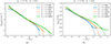 |
Fig. 1. Density (left) and temperature (right) profiles of a 1 M⊙ MS star of different models (see Table 1). The dashed and solid lines represent the 1D profiles generated by MESA and initialized (and subsequently relaxed for five dynamical timescales) in 3D in AREPO, respectively. They agree very well over most of the range, except close to the stellar surface because of smoothing during relaxation in AREPO. An older MS star (with lower Hc) has a denser and hotter core and a puffier outer layer than a younger MS star (with higher Hc). |
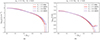 |
Fig. 2. Similar profiles to Fig. 1, but for a 0.5 M⊙ MS star. A 0.5 M⊙ star with an age of ∼13.5 Gyr with Hc = 0.60 (purple curves) is very similar to a ZAMS star with Hc = 0.70 (red curves), albeit with a slightly larger radius. |
2.3. Black hole
The black holes are initialized in AREPO as nonrotating sink particles that interact gravitationally and grow in mass through accretion. We set the gravitational softening length of the BH to be ten times the minimum softening length of the gas (star) cells. The scheme we used for accretion onto the BH, described here briefly, is the same as the one used in Ryu et al. (2022, 2023a,b, 2024a). Firstly, the cells around the BH within a radius of 104 rg, where the gravitational radius is rg = GmBH/c2, are identified. Secondly, the accretion onto the BH is calculated using a weighted average of radial flux to account for the higher contribution of gas closer to the BH and vice versa. Thirdly, mass is extracted from the neighboring cells of the BH, and momentum is inserted in the BH to conserve these quantities. Finally, the BH is spun up from accretion by adding angular momentum from the selected neighboring cells. The radiation feedback from accretion is not taken into account. Although angular momentum is conserved through this scheme, there is no guarantee that the total energy is conserved. However, given that accretion onto the black hole is small in our simulations, the energy lost due to accretion is negligible.
We ran simulations with SBH masses of 10 M⊙ and 40 M⊙, which are in proximity to the lower and higher mass peaks of observed LIGO BH masses (e.g., Abbott et al. 2021, 2023). Given the mass of the BH mBH, the mass of the star m⋆, and the radius of the star r⋆, the classical tidal radius is defined as rt = (mBH/m⋆)1/3r⋆.
2.4. Initial conditions
The distance of the closest approach is characterized by the impact parameter, b ≡ rp/rt1, where rp is the periapsis distance of the initially parabolic orbit. We varied the mass of the star (0.5 M⊙ and 1 M⊙) and the mass of the black hole (10 M⊙ and 40 M⊙). We then generated a suite of simulations of b varying from 0.25 to 2.00 (1 M⊙ stars) or 2.50 (0.5 M⊙ stars), and the three stellar ages (density profiles) to determine the post-disruption orbital, mass, and spin parameter. The additional simulations for 0.5 M⊙ and b = 2.50 are performed to properly analyze the PTDE trends since 0.5 M⊙ stars are fully disrupted for b ≲ 1.00.
We also assume that the initial stars are nonrotating and that the star-BH encounters are parabolic. This can be justified for encounters in globular clusters because the velocity dispersions of Milky Way globular clusters are in the ∼1 − 20 km s−1 range (e.g., Baumgardt & Hilker 2018). For instance, given a velocity dispersion of σ ≃ 10 km s−1, |1 − e|≃10−4 (very close to parabolic) for the parameters considered in this paper.
Each simulation was run for ∼70 tdyn, ⋆ after periapsis passage. This duration was chosen to ensure that the stellar masses reach steady values that would allow proper analysis. Table 2 provides an overview of the parameters we used in our suite of simulations.
Initial parameters of our suite of simulations.
3. Analysis
3.1. Calculation of bound and unbound mass
To find the center of mass of a self-bound object (i.e., star before disruption, remnant after disruption) in each snapshot, we used an iterative procedure fairly similar to that of Guillochon & Ramirez-Ruiz (2013), with some differences to improve the accuracy of the identification of bound and unbound cells. For each snapshot, we chose the gas cell with the maximum density as the “initial” guess for the center of mass (CoM) position. Subsequently, we calculated the specific total energies of all the star cells relative to the star’s CoM, εcell, CoM, and to the BH, εcell, BH, as the sum of their relative kinetic, potential, and internal energies. We consider a cell to be bound to a self-gravitating object if εcell, CoM < 0, εcell, CoM < εcell, BH. The last condition ensures that the cells bound to the star are “close” to the CoM. We computed a “new” CoM position (and velocity) using these bound cells and determined the new specific energy. We iterated this process until there was no change in the relative position of the CoM. Subsequently, we calculated its final bound mass. In the case of an FTDE, we also visually inspected the surface density plots and assigned the mass bound to the star to be zero.
The mass bound to the BH is calculated in a similar fashion, though the position of the BH is trivially known from the simulation. Finally, we consider any cells with εcell, CoM ≥ 0 and εcell, CoM ≥ 0 unbound from the system.
3.2. Calculation of orbital and spin parameters
For each post-disruption snapshot, we computed the instantaneous Keplerian orbital parameters – the semimajor axis a and orbital eccentricity e – using the current values of the mass bound to the star m⋆, the mass of the BH (plus the gas mass bound to it) mBH, the positions and velocities of the star’s CoM (rCoM, vCoM) and the BH (rBH, vBH). For completeness, with r ≡ rCoM − rBH and v ≡ vCoM − vBH, the equations are as follows:
 (1)
(1)
 (2)
(2)
We determine the spin angular momentum L⋆ about the star’s CoM using the masses mi, relative positions ri, and velocities vi of the bound gas cells. In the cases of full disruption, we ignored the orbital and spin parameters.
The final post-disruption mass, orbital, and spin parameters reported in the following section are the means and standard deviations of these quantities during the last ten snapshots of each simulation (the time between consecutive snapshots was chosen to be approximately equal to the initial dynamical timescale of the star). In the cases where a partially disrupted star returns on a second passage within the simulation time, we chose snapshots close to the apoapsis of the first passage for the parameter calculations.
4. Results
Figure 3 shows selected snapshots of our suite of simulations. It can be visually seen that the final outcomes (FTDE or PTDE) depend on all the parameters that we considered: the stellar mass m⋆, the core hydrogen fraction Hc, the BH mass mBH, and the impact parameter b.
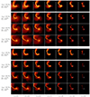 |
Fig. 3. Grid of log density slices of stars of ∼20 tdyn, ⋆ after undergoing μTDEs, with the BH at the center of each panel. Each row is for a different mBH (top and bottom half for 10 M⊙ and 40 M⊙, respectively), m⋆, or Hc, whereas the columns represent increasing b (from left to right). The dashed and solid circles around the BH, most visible in the rightmost panels, denote the tidal radius, rt, and the periapsis distance, rp, respectively. We note that the spatial range of each panel is not the same. |
The following sections detail the quantitative results. It should be noted that, henceforth, initial star parameters are given the subscript ⋆ (e.g., m⋆, L⋆), while the post-disruption remnant parameters are given the subscript ⋄ (e.g., m⋄, L⋄). Table A.1 provides detailed initial and post-disruption parameters for our 58 simulations.
4.1. Effect of density concentration factor
Ryu et al. (2020b) showed that, in the case of SMBHs, the critical impact parameter for full disruption, bFTDE, is inversely proportional to the density concentration factor  , where
  and ρc are the average and central stellar density, respectively (see also Law-Smith et al. 2020). A larger value of ρconc represents a denser core with a puffier outer layer, and vice versa. This indicates that a star with higher core density requires a smaller impact parameter to fully disrupt. Quantitatively, bFTDE can be written as
 (3)
(3)
Here,  is the critical impact parameter for the full disruption of a hypothetical star with uniform density, that is, ρconc = 1 (see also Eq. (15) of Ryu et al. 2020b). Table 3 displays the values of bFTDE of stars with polytropic indices γ (where P ∝ ργ) 4/3 and 5/3 as calculated by Mainetti et al. (2017). The analytically computed ρconc for these polytropes and the subsequently evaluated (using Eq. (3))
  values are also shown. We also estimate
  to be 1.95 ± 0.20 from our suite of simulations by fitting the remnant masses for given initial stellar and BH masses (see the following section for details) and find the values of bFTDE. Despite the significant difference in the masses of the black holes, our estimated values agree with those from Mainetti et al. (2017). Estimates of this factor calculated by Ryu et al. (2020b), Law-Smith et al. 2020, and Kıroğlu et al. (2023) all lie within the error range. Since the former two studies are on SMBHs and the latter is on IMBHs, we reiterate that
  is almost independent of the mass of the BH for a very large range of BH masses. The consensus between the previous works in spite of different numerical schemes (general relativistic grid-based hydrodynamics, adaptive-mesh refinement, and SPH) and the current work strengthens this point. Therefore, we use our computed value of
  for the fit functions in the following sections.
Evaluated values of the impact parameter for the full disruption of a star with uniform density,  .
.
For completeness, Fig. 4 (and Table 1) shows the trend  for MESA 1 M⊙ MS stars, with our three stellar models highlighted. We see that a more evolved star has a smaller
  (harder to fully disrupt) compared to a less evolved star (easier to fully disrupt) and that this relation is close to linear as a function of stellar age t⋆. Figure 5 shows the averaged
  values for a range of masses of MESA-generated MS stars (0.1 M⊙ − 20.0 M⊙) of two metallicities – 0.02 (near-solar) and 0.002 (sub-solar). We see that higher mass MS stars have denser cores and puffier outer layers (hence, lower
  values, which plateau for stars of masses ≳1 M⊙ at ∼1.6 − 2.0), while the opposite is true for lower mass MS stars. Moreover, metallicity affects
  only slightly, with the metal-poor stars being slightly less (more) centrally concentrated when m⋆ > 1.0 M⊙ (m⋆ ≤ 1.0 M⊙). The (approximate) values of
  are crucial to applying our fits (see the following sections).
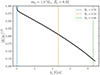 |
Fig. 4. MESA-derived inverses of density concentration factors |

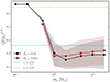 |
Fig. 5. MESA-derived inverses of density mean concentration factors |


4.2. Post-disruption stellar and BH masses
After a disruption event, a star loses mass, some of which becomes bound to (and eventually accreted onto) the BH, while the rest of it becomes unbound from the system. Evidently, the closer the approach of the star is to the BH, the larger the mass lost from the star.
Figure 6 shows this trend for the case of a 1 M⊙ (left) and a 0.5 M⊙ (right) star that is disrupted by a 10 M⊙ (top) and a 40 M⊙ (bottom) BH. The post-disruption fractional mass loss Δm⋄/m⋆, where Δm⋆ is the difference between the star’s initial mass m⋆ and the remnant mass m⋄. It decreases almost exponentially with the impact parameter b. Moreover, a more evolved MS star loses less mass compared to a less evolved star for the same value of b. This is because a more evolved star, with a higher central concentration, requires a stronger tidal force (or smaller b) to strip the same amount of mass when compared to a less evolved star. Consequently, bFTDE, corresponding to Δm⋄/m⋆ = 1, is also lower for more evolved stars.
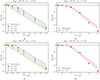 |
Fig. 6. Post-disruption fractional mass loss, Δm⋄/m⋆, for a star of mass 1 M⊙ (left) and 0.5 M⊙ (right), due to a BH of mass 10 M⊙ (top) and 40 M⊙ (bottom), as a function of impact parameter b and MS age (Hc abundance). The dashed line at the top signifies the full disruption of the star. The fractional mass losses are largely independent of BH mass. Mass loss is higher for lower b values, and this decreases roughly exponentially (best-fit lines and standard error regions shown) with increasing b. A less evolved star (higher Hc) loses more mass for the same value of b. A 0.5 M⊙ star has a higher mass loss than a 1 M⊙ star for the same b. |
Furthermore, we see that roughly half the mass lost from the star stays bound to the BH, although this is not always true, especially when there is little mass loss (see Table A.1). This bound mass decreases through time due to continuous debris interaction resulting in mass unbinding, and hence it is an upper limit for the mass that can be accreted onto the BH. Details of the accretion process and feedback from the BH might prevent some of the mass bound to the BH from being accreted, but following this process is beyond the scope of our paper. The other half of the stripped mass is unbound from the BH-star system.
We can fit (with standard 1σ errors) the fractional mass loss Δm⋆ well by
 (4)
(4)
Here, bFTDE is as given in Eq. (3). Since ρconc is taken into account, this fit differs from those obtained by Guillochon & Ramirez-Ruiz (2013) and Ryu et al. (2020c) for TDEs due to SMBHs. The remnant mass fit function does not explicitly depend on m⋆ and mBH, but only on b and ρconc. Since ρconc is higher for more evolved stars, they have a smaller bFTDE and, hence, less fractional mass loss. Figure 6 plots these best-fit curves, with the error bars shaded. It should be noted that this trend may not hold for larger values of b.
4.3. Post-disruption stellar spins
An initially nonrotating star gains spin after a tidal encounter due to tidal torques from the BH. Although we do not delve into the details of the spin-up, this results in differential, and not rigid, rotation of the star. It should be noted that, due to spurious motions in our initial AREPO stellar models, the spin angular momenta L⋆ are not zero but ∼1 − 2 × 1047 g cm2 s−1 (∼2 × 1046 g cm2 s−1) for 1 M⊙ (0.5 M⊙) stars. Since these values correspond to negligible equatorial surface velocities2 of ∼10 m s−1, the stars are considered to be nonrotating. The spin angular momentum of the remnant L⋄ depends on the internal structure of the original star and the impact parameter.
Figure 7 shows the trend of L⋄ with respect to the impact parameter b for the case of a 1 M⊙ (left) and a 0.5 M⊙ (right) star being partially disrupted by a 10 M⊙ (top) and a 40 M⊙ (bottom) BH. In addition, we indicate the approximate order-of-magnitude estimates of the break-up angular momenta (assuming uniform density and rigid rotation) of the remnant stars, L⋄, break = 0.4 m⋄r⋄v⋄, break3. Here, we crudely estimate the remnant radius as (r⋄/R⊙) = (m⋄/M⊙)0.7 and assume the break-up velocity to be the Keplerian velocity at r⋆, that is,  . In reality, the remnant is significantly puffed up, and the break-up velocity would depend on the true moment of inertia of the remnant (and thus, its density profile) and the differential rotation due to spin-up. For our range of simulation parameters, L⋄ remains below L⋄, break, although significant mass loss can bring the remnant very close to break-up, for example, m⋆ = 0.5 M⊙ and b ≲ 1.00. For higher values of b (but still less than b ∼ 2), L⋄ decreases almost exponentially as b increases. On the other hand, when b is less such that a fractional mass loss is ≥ 2 × 10⁻¹, the trend reverses until FTDE. This trend reflects the counter-balance between mass loss and spin-up: for stronger PTDEs, although the remnant is spun up more rapidly, the remnant mass is smaller.
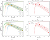 |
Fig. 7. Post-disruption spin angular momentum, L⋄, for an initially nonrotating star of mass 1 M⊙ (left) and 0.5 M⊙ (right), due to a BH of mass 10 M⊙ (top) and 40 M⊙ (bottom) and as a function of impact parameter b and MS age (Hc abundance). The dashed lines indicate the (approximate) estimated break-up angular momenta of the remnants L⋄, break, respectively. The spin angular momenta are largely independent of BH mass. It decreases almost exponentially for sufficiently high b values, and it drops for very low b values when the remnant mass is small (best-fit lines and standard error regions shown). The drop-off of angular momentum occurs at larger b for a less evolved star. |
The large spin-up for smaller b indicates that the specific angular momentum monotonically increases as b decreases. Motivated by this, we considered the scaled (moment-of-inertia-adjusted) parameter  . Here, the fractional remnant mass m⋄, frac ≡ m⋄/m⋆ and the post-disruption estimated fractional radius
  is a crude estimate of the radius of an MS star.
We found the following exponential fit (with standard 1σ errors) describes L⋄, scaled well:
 (5)
(5)
From the definition of  before, we have
 (6)
(6)
Here, (Δm⋄/m⋆) is estimated using Eq. (4). This equation implies that the post-disruption spin depends significantly on the fractional mass loss. Moreover, there is no dependence on mBH. Figure 7 plots these best-fit curves, with the error bars shaded.
4.4. Post-disruption orbital parameters
Depending on the stellar structure and the BH mass, a star in an initially parabolic orbit ends up in an eccentric or even a hyperbolic orbit after a PTDE (see also Ryu et al. 2020c; Kremer et al. 2022; Kıroğlu et al. 2023). The specific orbital energy of the star-BH system, εorb, is the sum of the specific energy injected into stellar tides, εtide, the specific binding energy of the ejected material, εbind, and the specific “kick” energy, εkick (see Kremer et al. 2022). Manukian et al. (2013) estimated the potentially unbinding kick received by a star undergoing PTDE due to an SMBH from asymmetric mass loss and observed that it depends solely on the mass loss and not on the star-SMBH mass ratio. However, this is not true for μTDEs – the mass ratio determines the kick, and hence the boundedness, of the star-SBH system (see also Fig. 2 of Kıroğlu et al. 2023 for TDEs due to IMBHs).
Figure 8 shows the post-disruption specific orbital energy of the star-BH system, εorb, for the disruption of a 1 M⊙ and a 0.5 M⊙ star by a 10 M⊙ (top panel) and a 40 M⊙ (bottom panel) BH. The values are normalized to the square of σ = 10 km s−1, which is the typical velocity dispersion of Milky Way globular clusters (e.g., Baumgardt & Hilker 2018). More negative (positive) values represent more bound (unbound) orbits. In general, εorb becomes more negative with decreasing b. If the density concentration factor ρconc is high enough (as in the case of a TAMS 1 M⊙ star; see Fig. 4), this trend continues until FTDE. However, in the case of a ZAMS 1 M⊙ star (and less extremely in a MAMS star), there is a certain value of b at which εorb starts to increase with decreasing b. This is due to the momentum kick from asymmetric mass loss, which becomes significant when the mass loss is high. In the case of a PTDE of a 1 M⊙ ZAMS star by a 40 M⊙ BH, the post-disruption orbit can be hyperbolic (unbound) for b values close to FTDE. This trend is more extreme for a 0.5 M⊙ star, with hyperbolic orbits being possible even in the case of PTDE by a 10 M⊙ BH. Moreover, their velocities at infinity are high enough (∼100 − 300 km s−1) to escape the cluster entirely. The two different BH masses result in quite different quantitative orbital parameters. Similarly to Kremer et al. (2022), we can write each of the energy components as follows:
![Mathematical equation: $$ \begin{aligned}&\varepsilon _{\mathrm{tide} } = - \frac{G m_{\mathrm{BH} }^2}{r_{\star } m_{\diamond }} \left[\left(\frac{r_{\star }}{r_{\mathrm{p} }}\right)^6 T_2 + \left(\frac{r_{\star }}{r_{\mathrm{p} }}\right)^8 T_3\right],\end{aligned} $$](/articles/aa/full_html/2024/05/aa48357-23/aa48357-23-eq36.gif) (7)
(7)
 (8)
(8)
 (9)
(9)
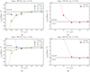 |
Fig. 8. Post-disruption normalized specific orbital energies of the star-BH system, εorb, for a star of mass 1 M⊙ (left) and 0.5 M⊙ (right) initially in a parabolic orbit, due to a BH of mass 10 M⊙ (top) and 40 M⊙ (bottom), as a function of impact parameter b and MS age (Hc abundance). The dashed line represents parabolic orbits and separates the parameter space into bound (eccentric) and unbound (hyperbolic) orbits. When mass loss is relatively low, a lower value of b generally results in more negative εorb in the case of 1 M⊙ star. This trend continues for the TAMS star. However, for the ZAMS and MAMS stars, significant mass losses can reverse this trend, with hyperbolic orbits also being a possibility (e.g., 1 M⊙ ZAMS star and 40 M⊙ BH mass with b < 1.00) 0.5 M⊙ stars, on the other hand, can become unbound for larger b, with boundedness also depending on the mass of the BH. |
Here, T2 and T3 are terms that depend on the stellar mass, radius, and density structure; BH mass; and approach distance (Press & Teukolsky 1977; Lee & Ostriker 1986). For the range of parameters considered, with mBH > m⋆ and rp ∼ r⋆, the values of T2 and T3 lie in the 0.01 − 0.1 range. These values are systematically lower for stars with lower ρconc values. As a result, in 0.5 M⊙ stars (and ZAMS 1 M⊙ stars), εtide is dominated by εkick, resulting in them becoming unbound from the BH. It should be noted that εtide depends very strongly on the distance of approach.
In addition, we find that the change in the specific orbital angular momentum of the star-BH system, horb, is not significant. For orbits very close to being parabolic, which is the case for all our post-disruption orbits (see Fig. 9),  . This implies that the post-disruption periapsis distance, rp = a(1 − e), where a is the semimajor axis and e is the eccentricity, is nearly the same as the initial periapsis distance, rp ≡ brt, which is also seen in PTDEs by SMBHs (Ryu et al. 2020c). Consequently, given that a = −0.5 G(m⋆ + mBH)/εorb, the calculation of e is straightforward. Figure 9 shows the post-disruption e, computed using Eqs. (1) and (2), as a function of b which follows the trend in εorb.
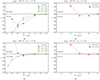 |
Fig. 9. Post-disruption orbital eccentricities, e, for a star of mass 1 M⊙ (left) and 0.5 M⊙ (right) initially in a parabolic orbit, due to a BH of mass 10 M⊙ (top) and 40 M⊙ (bottom) and as a function of impact parameter b and MS age (Hc abundance). The dashed line represents parabolic orbits and separates the parameter space into bound (eccentric) and unbound (hyperbolic) orbits. The reason for the trends is the same as that for Fig. 8. |
4.5. Rates of tidal encounters
The rate of μTDEs per year per Milky Way-like galaxy (similar to Perets et al. 2016) can be expressed as
 (10)
(10)
Here, Nclus ∼ 150 MWGal−1 is the number of globular clusters (in the Milky Way; e.g., Harris 2010), N⋆, c is the number of stars in a cluster core, NBH, c is the number of BHs in a cluster core,  is the gravitational focused encounter cross-section with periapsis distance rp = brt (see Sect. 2) and periapsis velocity
  , and σ is the velocity dispersion of the cluster. For globular clusters in the Milky Way Galaxy, the typical values of these parameters are
  pc−3 (e.g., Baumgardt & Hilker 2018), NBH, c ∼ 10 − 100 (e.g., Morscher et al. 2015; Askar et al. 2018), σ ∼ 1 − 20 km s−1 (e.g., Baumgardt & Hilker 2018). With these values, and assuming vp ≫ σ in globular clusters, and typical star and BH masses of 1 M⊙ and 10 M⊙ respectively, the rate is
 (11)
(11)
This equation implies that PTDEs (with larger rp/rt) are more frequent than FTDEs. More specifically, from our simulations of TDEs of 1 M⊙ stars by 10 M⊙, encounters with b ∼ 1 − 2 would result in eccentric bound orbits, which can circularize over time through tides. A more detailed rate calculation would involve integrating Eq. (11) over a range of star and black hole masses.
The above rates are derived for μTDEs produced in dense stellar systems such as globular clusters and nuclear star clusters. However, other channels also contribute to μTDEs (see discussion in Perets et al. 2016), such as ultra-wide binaries and triples in the field (Michaely & Perets 2016, 2020) and post-natal-kicks leading to a close encounter between a newly formed BH and a stellar companion (Michaely et al. 2016). These channels may give rise to μTDEs in young environments and in the field.
4.6. Summary of fits
Below, we present the post-disruption fits detailed in previous sections for use in globular cluster codes. m⋆ → BH refers to the gas mass bound to the black hole after disruption, including the accreted mass.
Masses of remnant star and BH:
 (12)
(12)
 (13)
(13)
Spin of remnant star:
 (14)
(14)
4.6.1. Validity of fits
It should be noted that the density concentration factor, ρconc, only captures the full disruption of a star. Similarly defined factors for each radius r, i.e.  , are required to calculate the distance at which mass beyond r is lost (see Ryu et al. 2020b). Stars of higher masses tend to have much steeper density profiles when compared to 1 M⊙ stars; thus, Eq. (4), which fits the mass loss, is not universal. In particular, the mass-loss fit for 2 M⊙ stars would involve an exponent of ∼3, unlike our derived exponent of ∼2.1 in Eq. (4). Similar arguments follow for the fits of spins and orbits.
5. Implications
In this section, we discuss the general observational implications and the caveats of our study. μTDEs can potentially produce both unique and peculiar transient events as well as longer lived systems.
5.1. Low-mass X-ray binaries
Low-mass X-ray binaries (LMXBs) are interacting binary systems that consist of compact objects (neutrons stars or black holes) accreting mass from their low-mass (≲1 M⊙) stellar companions, thereby producing X-rays. A few hundred LMXBs have been detected in the Milky Way (e.g., Liu et al. 2007; Avakyan et al. 2023), highlighting the prevalence of such systems. However, theoretical (e.g., Portegies Zwart et al. 1997; Kalogera 1999) and population synthesis (e.g., Podsiadlowski et al. 2003; Kiel & Hurley 2006) studies have not been able to match the rates of observed LMBXs through isolated binary evolution alone. The primary reason is that a low-mass companion has insufficient energy to expel a common envelope during the giant phase of the primary star, thereby resulting in the spiraling in of the companion and an eventual merger. Thus, a dynamical channel formation channel for LMXBs, where a low-mass star is tidally captured by a black hole in a globular or nuclear cluster, is promising (e.g., Voss & Gilfanov 2007; Michaely & Perets 2016; Klencki et al. 2017).
Some of our simulations of encounters of low-mass stars with black holes are not close enough for significant mass loss and can result in highly eccentric bound orbits. For example, in the parabolic encounter of a 1 M⊙ star and a 10 M⊙ BH, for b ∼ 1.0 − 1.5 (see Sect. 4), the fractional mass loss is ∼1 − 10% and the post-disruption bound orbit has a period of 0.1 − 1 yr and an eccentricity of ∼0.97 − 0.98. However, tidal dissipation at subsequent periapsis passages can reduce the eccentricity and orbital period (e.g., Klencki et al. 2017) such that the resulting bound system evolves into a compact LMXB.
Another type of system that is potentially formed through dynamical encounters are non-interacting BH-star systems (e.g., El-Badry et al. 2023a,b; Chakrabarti et al. 2023). These systems consist of ∼1 M⊙ stars orbiting ∼10 M⊙ black holes in moderately-eccentric orbits with periods of ∼1 yr. These parameters correspond quite well with our simulations with b ∼ 1.0 − 1.5, which lends credence to dynamical formation.
5.2. Intermediate-mass black-hole growth
Intermediate-mass black holes (IMBHs; see Greene et al. 2020 for a review), with masses greater than those of stellar-mass black holes (≳102 M⊙) and less than those of supermassive black holes (≲106 M⊙), are expected to exist in the centers of dwarf galaxies (e.g., Kunth et al. 1987; Filippenko & Sargent 1989; Reines 2022; Gültekin et al. 2022) and globular clusters (e.g., Davis et al. 2011; Farrell et al. 2014; Pechetti et al. 2022). Among several IMBH formation mechanisms (see Volonteri et al. 2021 for review), one possible avenue is runaway mass growth through tidal capture and disruption, which has been examined analytically (e.g., Stone et al. 2017) and numerically (e.g., Rizzuto et al. 2023; Arca Sedda et al. 2023). One of the most critical factors in this mechanism for BH growth is the amount of debris mass that ultimately accretes onto the BH. For example, Rizzuto et al. (2023) assumed that a star approaching a BH within the nominal tidal radius rt is fully destroyed and 50% of the stellar mass is accreted onto the BH.
While these assumptions may be valid for a part of the parameter space, it is important to develop a prescription for the outcomes of TDEs that works over a broader parameter range to more accurately assess the possibility of BH mass growth through TDEs. Our simulations can provide such prescriptions that can improve the treatment of TDEs. Firstly, our simulations show, as previous work on TDEs by supermassive black holes (e.g., Guillochon & Ramirez-Ruiz 2013; Mainetti et al. 2017; Goicovic et al. 2019; Ryu et al. 2020a,b,c,d; Law-Smith et al. 2020), that the periapis distances at which stars are fully or partially destroyed depend on the stellar internal structure. Ryu et al. (2020b) analytically demonstrated that the nominal tidal radius rt is a more relevant quantity for partial disruption events involving stars with m⋆ ≳ 1 M⊙. Only for lower-mass stars, where ρconc ∼ 1, does rt come close to the genuine full disruption radius4. Our fitting formula for the fractional mass loss, Eq. (4), can provide a better prescription for determining the fate of the star (full or partial disruption) as well as the mass of the remnant.
The amount of debris accreted onto the BH remains highly uncertain. To the zeroth order, if the accretion rate is super-Eddington, the strong radiation pressure gradient would drive strong outflows, hindering continuous and steady accretion (Sądowski et al. 2014). However, the accretion efficiency would be collectively affected by many factors, including magnetic fields, black hole spins, accretion-flow structure, and jet formation (e.g., Sądowski et al. 2014; Jiang et al. 2019; Curd & Narayan 2023; Kaaz et al. 2023). Our fitting formulae for the fractional mass loss cannot provide an accurate prescription for the accreted mass, but they can place constraints on the maximum mass that can be accreted onto the BH.
5.3. Fast blue optical transients
Fast blue optical transients (FBOTs) are a class of optical transients characterized by high peak luminosities > 1043 erg s−1, rapid rise and decay times on the order of a few days, blue colors (Perets et al. 2011; Drout et al. 2014), and peak black-body temperatures of a few 104 K. Although a majority of these events can be explained by supernovae with low-mass ejecta (Pursiainen et al. 2018), a “luminous” subset, for example, AT2018cow (the Cow; Smartt et al. 2018; Prentice et al. 2018), AT2018lqh (Ofek et al. 2021), AT2020mrf (Yao et al. 2022), CSS161010 (Coppejans et al. 2020), ZTF18abvkwla (the Koala; Ho et al. 2020), AT2020xnd (the Camel; Perley et al. 2021), AT2022tsd (the Tasmanian Devil; Matthews et al. 2023), and AT2023fhn (the Finch; Chrimes et al. 2024), are too bright at their peaks and fade too rapidly to be explained by supernovae. Proposed mechanisms involve compact objects, such as BH accretion or magnetars formed in core-collapse supernovae (Prentice et al. 2018), mergers between Wolf-Rayet stars and compact objects accompanied by hyper-accretion (Metzger 2022), or tidal disruption events by intermediate-mass BHs (Kuin et al. 2019) or stellar-mass BHs (Kremer et al. 2021).
Some luminous FBOTs also emit in the radio or X-ray (e.g., Margutti et al. 2019; Ho et al. 2020), which indicates the presence of a circumstellar medium that may result from partial TDEs (Kremer et al. 2021). Our simulations support this notion by showing the presence of debris near the BH with occasional weak outflows from the BH. In addition, the remnants in our simulations are often bound to the BH and can subsequently undergo multiple partial disruptions, for example, our simulations of TAMS 1 M⊙ stars and 10 M⊙ BHs for b = 0.25 or b = 0.33. While we cannot confirm a direct correlation between FBOTs and μTDEs, multiple disruption events of a star may fulfill some of the astrophysical conditions (e.g., the presence of a gas medium and rapid accretion onto a compact object) necessary to explain FBOTs with radio emission. For such cases, the detection of repeated bursts in FBOTs could provide valuable constraints on their formation mechanisms.
5.4. Ultra-long gamma-ray bursts and X-ray flares
The exact appearance of transients resulting from μTDEs is highly uncertain and depends on various assumptions. Perets et al. (2016) suggested that if the accretion onto the BH is efficient and gives rise to jets, there is a possibility of producing ultra-long gamma-ray bursts (GRBs) and/or X-ray flares (XRFs).
Assuming a proportional relation between the material accreted to the compact object and the luminosity produced by the jet, we can generally divide μTDEs into two regimes: (1) tmin ≫ tacc and (2) tmin ≪ tacc, where tmin is the typical fallback time of the debris following the disruption, and tacc is the typical viscous time of the accretion disk that can form around the BH (see Perets et al. 2016 for more details). We descrbe these regimes below:
-
tmin ≫ tacc: when the mass of the star is much smaller than that of the BH, the accretion evolution is dominated by the fallback rate; that is, the light curve should generally follow the regular power law (e.g., t−5/3 power-law for a full disruption).
-
tmin ≪ tacc: when the masses of the star and the BH are comparable, the fallback material is expected to accumulate and form a disk on the fallback time, which then drains on the longer viscous time, maintaining a low accretion rate. We would expect the flaring to begin only once the material is accreted onto the compact object. Therefore, we expect four stages in the light curve evolution. These are as follows: (1) a fast rise of the accretion flare once the disk material is processed and evolves to accrete on the compact object; (2) accretion from the disk until the accumulated early fall-back material is drained (if we assume a steady state accretion until drainage, one might expect a relatively flat light curve); (3) a steep drop in the light curve once the disk drains the accumulated early fall-back material. Finally, (4) the continuous fall-back of material would govern the accretion rate at times longer than the viscous time, and the accretion rate should then follow the t−5/3 rate (or a different power law). The exact light curve at the early stages is difficult to predict, but we do note a non-trivial signature of the μTDEs relating to the early and late stages.
The expected properties of μTDEs are consistent with and might explain the origins of ultra-long GRBs (Levan et al. 2014): long-lived (∼104 s) GRBs that show an initial plateau followed by a rapid decay. μTDEs may also explain the origin of some Swift TDE candidates (Bloom et al. 2011; Burrows et al. 2011; Cenko et al. 2012; Brown et al. 2015), which are suggested to be produced through a TDE by a supermassive BH. The typical timescales for the latter are longer than the observed 105 s, challenging the currently suggested origin, but quite consistent with a μTDE scenario.
μTDEs producing ultra-long GRBs are also expected to produce afterglow emission if or when the strong outflows and jets launched by accretion propagate into the surrounding medium, and the resulting shock interaction produces high energy particles, which give rise to synchrotron and inverse Compton radiation. Such an observational signature of μTDE has been little explored, though analogous observation and modeling have been suggested for TDEs by massive BHs (e.g., Giannios & Metzger 2011; Zauderer et al. 2011). Detection of afterglows from μTDEs would provide information on the energetics and dynamics of the outflow, robust independent evidence for the jet collimation, and the identification of the host galaxy.
5.5. Remnants
Partial μTDEs of stars by stellar BHs can spin up the stars significantly due to strong tidal interactions (see Fig. 7 and Alexander & Kumar 2001). Though magnetic breaking can potentially spin down such stars over time, observations of old, highly spun-up low-mass stars in globular clusters could provide potential signatures for partial μTDEs. In addition, the remnant undergoes violent chemical mixing during the first pericenter passage and has higher entropy than an ordinary star of the same mass and age (Ryu et al. 2020c, 2023a). If the mass loss is significant, a unique chemical composition profile may persist even after the remnant has relaxed to a stable state. This suggests that the remnant could exhibit unique asteroseismic signatures that distinguish it from ordinary stars (Bellinger et al., in prep.).
5.6. Caveats
As mentioned in Sect. 2, we exclude the effects of relativity and magnetic fields in our study. The Newtonian approximation is justified for TDEs by SBHs because most of the debris stays outside rp, which is approximately four orders of magnitude greater than the gravitational radius rg ≡ GmBH/c25. However, relativistic effects and proper treatment of radiation are more important for the accretion flow, which is beyond the scope of our paper. The effect of magnetic fields on the dynamics of the remnant is unclear, and we leave this area of study for our future work. A final point to note is that, unlike globular clusters, nuclear star clusters have typical velocity dispersions of σ ≳ 100 km s−1 (Figer et al. 2003; Schödel et al. 2009) depending on the galaxy and, subsequently, |1 − e|≳10−2. Thus, encounters are not always parabolic, and for a more thorough study, hyperbolic encounters must be taken into account.
6. Summary and conclusion
We performed a grid of 58 hydrodynamics simulations, using the moving-mesh code AREPO, of partial and full tidal disruptions of main-sequence stars with stellar-mass black holes on initially parabolic orbits. Our varied parameters include stellar mass m⋆ (0.5 M⊙ and 1.0 M⊙), SBH mass (10 M⊙ and 40 M⊙), core hydrogen abundance Hc (a proxy for MS age t⋆), and impact parameter b ≡ rp/rt. Our stellar models are initialized in accordance with 1D detailed nonrotating stellar profiles from MESA. We also define a star’s density concentration parameter  . Our main results are summarized below.
-
The mass of a post-disruption stellar remnant, m⋄, decreases with decreasing b. A higher ρconc (more centrally concentrated) results in a lesser mass loss for the same b. m⋄ only depends on b and ρconc and not on mBH. Roughly half of the disrupted mass remains bound to the black hole, while the other half is unbound from the system.
-
The spin angular momentum of a stellar remnant L⋄ increases after periapsis passage. For large b (when the mass loss is small), L⋄ increases with decreasing b, but this trend reverses for very small b (close to FTDE) due to significant mass loss. This reversal occurs for lower b when ρconc is higher. The final spin is also independent of mBH. For low b values, the rotational velocities can be very close to break-up velocities.
-
Unlike mass and spin, the orbit of the remnant star also depends on mBH. For large b, the eccentricity e and semimajor axis a decrease with decreasing b, keeping a constant periapsis distance; that is, the remnant tends to be more “bound”. Depending on mBH and ρconc, this no longer holds for approaches close to FTDE – e can increase and the remnant can become unbound. In general, a higher mBH/m⋆ ratio and a lower ρconc tend to be unbinding.
-
We provide relatively simple and accurate fitting formulae for the masses and spins of the remnant stars. These analytical fits are listed in Sect. 4.6 for easy access.
We discussed the implications that μTDEs can have on low-mass X-ray binary formation, intermediate-mass black hole formation, and transient searches. Given the limited range of stellar masses and ages that we covered in this work, we will extend our suite of simulations in the future to cover a wider parameter space, including massive stars. It is necessary to explore this regime to model stellar dynamics in dense stellar clusters.
β ≡ b−1 is often introduced in the literature for TDEs by SMBHs as the “penetration factor”.
In contrast, the Sun, a very slow rotator, has an equatorial surface velocity of ∼2 km s−1.
This is because a hypothetical star (sphere) of uniform density has a moment of inertia of  about an axis of rotation passing through the center.
The genuine full disruption radius and the partial disruption radius are proportional to  and
and  respectively (see Sect. 4 of Ryu et al. 2020b).
On the other hand, for TDEs with SMBHs, rg and rt can be comparable in scale.
Acknowledgments
The authors thank Thorsten Naab for useful discussions regarding star-black hole encounters in star clusters. P.V. acknowledges the computational resources provided by the Max Planck Institute for Astrophysics to carry out this research.
References
- Abbott, R., Abbott, T. D., Abraham, S., et al. 2021, ApJ, 913, L7 [NASA ADS] [CrossRef] [Google Scholar]
- Abbott, R., Abbott, T. D., Acernese, F., et al. 2023, Phys. Rev. X, 13, 011048 [NASA ADS] [Google Scholar]
- Alexander, T., & Kumar, P. 2001, ApJ, 549, 948 [NASA ADS] [CrossRef] [Google Scholar]
- Arca Sedda, M., Kamlah, A. W. H., Spurzem, R., et al. 2023, MNRAS, 526, 429 [NASA ADS] [CrossRef] [Google Scholar]
- Askar, A., Arca Sedda, M., & Giersz, M. 2018, MNRAS, 478, 1844 [NASA ADS] [CrossRef] [Google Scholar]
- Avakyan, A., Neumann, M., Zainab, A., et al. 2023, A&A, 675, A199 [NASA ADS] [CrossRef] [EDP Sciences] [Google Scholar]
- Bagla, J. S. 2002, JApA, 23, 185 [NASA ADS] [Google Scholar]
- Baumgardt, H., & Hilker, M. 2018, MNRAS, 478, 1520 [Google Scholar]
- Bellm, E. C., Kulkarni, S. R., Graham, M. J., et al. 2019, PASP, 131, 018002 [Google Scholar]
- Bloom, J. S., Giannios, D., Metzger, B. D., et al. 2011, Science, 333, 203 [CrossRef] [PubMed] [Google Scholar]
- Brown, G. C., Levan, A. J., Stanway, E. R., et al. 2015, MNRAS, 452, 4297 [NASA ADS] [CrossRef] [Google Scholar]
- Burmester, U. P., Ferrario, L., Pakmor, R., et al. 2023, MNRAS, 523, 527 [NASA ADS] [CrossRef] [Google Scholar]
- Burrows, D. N., Kennea, J. A., Ghisellini, G., et al. 2011, Nature, 476, 421 [NASA ADS] [CrossRef] [Google Scholar]
- Cenko, S. B., Krimm, H. A., Horesh, A., et al. 2012, ApJ, 753, 77 [NASA ADS] [CrossRef] [Google Scholar]
- Chakrabarti, S., Simon, J. D., Craig, P. A., et al. 2023, AJ, 166, 6 [NASA ADS] [CrossRef] [Google Scholar]
- Chambers, K. C., Magnier, E. A., Metcalfe, N., et al. 2016, arXiv e-prints [arXiv:1612.05560] [Google Scholar]
- Chrimes, A. A., Jonker, P. G., Levan, A. J., et al. 2024, MNRAS, 527, L47 [Google Scholar]
- Coppejans, D. L., Margutti, R., Terreran, G., et al. 2020, ApJ, 895, L23 [NASA ADS] [CrossRef] [Google Scholar]
- Curd, B., & Narayan, R. 2023, MNRAS, 518, 3441 [Google Scholar]
- Davis, S. W., Narayan, R., Zhu, Y., et al. 2011, ApJ, 734, 111 [NASA ADS] [CrossRef] [Google Scholar]
- De Angeli, F., Piotto, G., Cassisi, S., et al. 2005, AJ, 130, 116 [NASA ADS] [CrossRef] [Google Scholar]
- Drout, M. R., Chornock, R., Soderberg, A. M., et al. 2014, ApJ, 794, 23 [Google Scholar]
- El-Badry, K., Rix, H.-W., Cendes, Y., et al. 2023a, MNRAS, 521, 4323 [NASA ADS] [CrossRef] [Google Scholar]
- El-Badry, K., Rix, H.-W., Quataert, E., et al. 2023b, MNRAS, 518, 1057 [Google Scholar]
- Farrell, S. A., Servillat, M., Gladstone, J. C., et al. 2014, MNRAS, 437, 1208 [CrossRef] [Google Scholar]
- Figer, D. F., Gilmore, D., Kim, S. S., et al. 2003, ApJ, 599, 1139 [NASA ADS] [CrossRef] [Google Scholar]
- Filippenko, A. V., & Sargent, W. L. W. 1989, ApJ, 342, L11 [NASA ADS] [CrossRef] [Google Scholar]
- Gallegos-Garcia, M., Law-Smith, J., & Ramirez-Ruiz, E. 2018, ApJ, 857, 109 [CrossRef] [Google Scholar]
- Gehrels, N., Chincarini, G., Giommi, P., et al. 2004, ApJ, 611, 1005 [Google Scholar]
- Gezari, S. 2021, ARA&A, 59, 21 [NASA ADS] [CrossRef] [Google Scholar]
- Giannios, D., & Metzger, B. D. 2011, MNRAS, 416, 2102 [NASA ADS] [CrossRef] [Google Scholar]
- Glanz, H., Perets, H. B., Pakmor, R. 2023, arXiv e-prints [arXiv:2309.03300] [Google Scholar]
- Goicovic, F. G., Springel, V., Ohlmann, S. T., & Pakmor, R. 2019, MNRAS, 487, 981 [NASA ADS] [CrossRef] [Google Scholar]
- Golightly, E. C. A., Nixon, C. J., & Coughlin, E. R. 2019, ApJ, 882, L26 [NASA ADS] [CrossRef] [Google Scholar]
- Greene, J. E., Strader, J., & Ho, L. C. 2020, ARA&A, 58, 257 [Google Scholar]
- Gronow, S., Collins, C. E., Sim, S. A., & Röpke, F. K. 2021, A&A, 649, A155 [NASA ADS] [CrossRef] [EDP Sciences] [Google Scholar]
- Guillochon, J., & Ramirez-Ruiz, E. 2013, ApJ, 767, 25 [NASA ADS] [CrossRef] [Google Scholar]
- Gültekin, K., Nyland, K., Gray, N., et al. 2022, MNRAS, 516, 6123 [CrossRef] [Google Scholar]
- Harris, W. E. 2010, arXiv e-prints [arXiv:1012.3224] [Google Scholar]
- Ho, A. Y. Q., Perley, D. A., Kulkarni, S. R., et al. 2020, ApJ, 895, 49 [NASA ADS] [CrossRef] [Google Scholar]
- Jansen, F., Lumb, D., Altieri, B., et al. 2001, A&A, 365, L1 [NASA ADS] [CrossRef] [EDP Sciences] [Google Scholar]
- Jiang, Y.-F., Stone, J. M., & Davis, S. W. 2019, ApJ, 880, 67 [Google Scholar]
- Kaaz, N., Murguia-Berthier, A., Chatterjee, K., Liska, M. T. P., & Tchekhovskoy, A. 2023, ApJ, 950, 31 [CrossRef] [Google Scholar]
- Kalogera, V. 1999, ApJ, 521, 723 [NASA ADS] [CrossRef] [Google Scholar]
- Kiel, P. D., & Hurley, J. R. 2006, MNRAS, 369, 1152 [NASA ADS] [CrossRef] [Google Scholar]
- Kıroğlu, F., Lombardi, J. C., Kremer, K., et al. 2023, ApJ, 948, 89 [CrossRef] [Google Scholar]
- Klencki, J., Wiktorowicz, G., Gładysz, W., & Belczynski, K. 2017, MNRAS, 469, 3088 [NASA ADS] [CrossRef] [Google Scholar]
- Kochanek, C. S., Shappee, B. J., Stanek, K. Z., et al. 2017, PASP, 129, 104502 [Google Scholar]
- Kollmeier, J., Anderson, S. F., Blanc, G. A., et al. 2019, BAAS, 51, 274 [NASA ADS] [Google Scholar]
- Kramer, M., Schneider, F. R. N., Ohlmann, S. T., et al. 2020, A&A, 642, A97 [NASA ADS] [CrossRef] [EDP Sciences] [Google Scholar]
- Kremer, K., Lu, W., Piro, A. L., et al. 2021, ApJ, 911, 104 [CrossRef] [Google Scholar]
- Kremer, K., Lombardi, J. C., Lu, W., Piro, A. L., & Rasio, F. A. 2022, ApJ, 933, 203 [NASA ADS] [CrossRef] [Google Scholar]
- Kuin, N. P. M., Wu, K., Oates, S., et al. 2019, MNRAS, 487, 2505 [NASA ADS] [CrossRef] [Google Scholar]
- Kunth, D., Sargent, W. L. W., & Bothun, G. D. 1987, AJ, 93, 29 [CrossRef] [Google Scholar]
- Law, N. M., Kulkarni, S. R., Dekany, R. G., et al. 2009, PASP, 121, 1395 [NASA ADS] [CrossRef] [Google Scholar]
- Law-Smith, J., Guillochon, J., & Ramirez-Ruiz, E. 2019, ApJ, 882, L25 [CrossRef] [Google Scholar]
- Law-Smith, J. A. P., Coulter, D. A., Guillochon, J., Mockler, B., & Ramirez-Ruiz, E. 2020, ApJ, 905, 141 [NASA ADS] [CrossRef] [Google Scholar]
- Lee, H. M., & Ostriker, J. P. 1986, ApJ, 310, 176 [CrossRef] [Google Scholar]
- Levan, A. J., Tanvir, N. R., Starling, R. L. C., et al. 2014, ApJ, 781, 13 [Google Scholar]
- Lioutas, G., Bauswein, A., Soultanis, T., et al. 2024, MNRAS, 528, 1906 [NASA ADS] [CrossRef] [Google Scholar]
- Liu, Q. Z., van Paradijs, J., & van den Heuvel, E. P. J. 2007, A&A, 469, 807 [NASA ADS] [CrossRef] [EDP Sciences] [Google Scholar]
- Lopez, M., Jr., Batta, A., Ramirez-Ruiz, E., Martinez, I., & Samsing, J. 2019, ApJ, 877, 56 [NASA ADS] [CrossRef] [Google Scholar]
- Mainetti, D., Lupi, A., Campana, S., et al. 2017, A&A, 600, A124 [NASA ADS] [CrossRef] [EDP Sciences] [Google Scholar]
- Manukian, H., Guillochon, J., Ramirez-Ruiz, E., & O’Leary, R. M. 2013, ApJ, 771, L28 [NASA ADS] [CrossRef] [Google Scholar]
- Margutti, R., Metzger, B. D., Chornock, R., et al. 2019, ApJ, 872, 18 [Google Scholar]
- Marín-Franch, A., Aparicio, A., Piotto, G., et al. 2009, ApJ, 694, 1498 [Google Scholar]
- Martin, D. C., Fanson, J., Schiminovich, D., et al. 2005, ApJ, 619, L1 [Google Scholar]
- Matthews, D., Margutti, R., Metzger, B. D., et al. 2023, Res. Notes Am. Astron. Soc., 7, 126 [Google Scholar]
- Metzger, B. D. 2022, ApJ, 932, 84 [NASA ADS] [CrossRef] [Google Scholar]
- Michaely, E., & Perets, H. B. 2016, MNRAS, 458, 4188 [NASA ADS] [CrossRef] [Google Scholar]
- Michaely, E., & Perets, H. B. 2020, MNRAS, 498, 4924 [NASA ADS] [CrossRef] [Google Scholar]
- Michaely, E., Ginzburg, D., & Perets, H. B. 2016, arXiv e-prints [arXiv:1610.00593] [Google Scholar]
- Morscher, M., Pattabiraman, B., Rodriguez, C., Rasio, F. A., & Umbreit, S. 2015, ApJ, 800, 9 [NASA ADS] [CrossRef] [Google Scholar]
- Ofek, E. O., Adams, S. M., Waxman, E., et al. 2021, ApJ, 922, 247 [NASA ADS] [CrossRef] [Google Scholar]
- Ohlmann, S. T., Röpke, F. K., Pakmor, R., & Springel, V. 2016a, ApJ, 816, L9 [Google Scholar]
- Ohlmann, S. T., Röpke, F. K., Pakmor, R., Springel, V., & Müller, E. 2016b, MNRAS, 462, L121 [NASA ADS] [CrossRef] [Google Scholar]
- Ohlmann, S. T., Röpke, F. K., Pakmor, R., & Springel, V. 2017, A&A, 599, A5 [NASA ADS] [CrossRef] [EDP Sciences] [Google Scholar]
- Ondratschek, P. A., Röpke, F. K., Schneider, F. R. N., et al. 2022, A&A, 660, L8 [NASA ADS] [CrossRef] [EDP Sciences] [Google Scholar]
- Pakmor, R., Kromer, M., Taubenberger, S., & Springel, V. 2013, ApJ, 770, L8 [Google Scholar]
- Pakmor, R., Springel, V., Bauer, A., et al. 2016, MNRAS, 455, 1134 [Google Scholar]
- Pakmor, R., Zenati, Y., Perets, H. B., & Toonen, S. 2021, MNRAS, 503, 4734 [Google Scholar]
- Pakmor, R., Callan, F. P., Collins, C. E., et al. 2022, MNRAS, 517, 5260 [NASA ADS] [CrossRef] [Google Scholar]
- Paxton, B., Bildsten, L., Dotter, A., et al. 2011, ApJS, 192, 3 [Google Scholar]
- Pechetti, R., Seth, A., Kamann, S., et al. 2022, ApJ, 924, 48 [NASA ADS] [CrossRef] [Google Scholar]
- Perets, H. B., Badenes, C., Arcavi, I., Simon, J. D., & Gal-yam, A. 2011, ApJ, 730, 89 [NASA ADS] [CrossRef] [Google Scholar]
- Perets, H. B., Li, Z., Lombardi, J. C., Jr., & Milcarek, S. R., Jr. 2016, ApJ, 823, 113 [NASA ADS] [CrossRef] [Google Scholar]
- Perley, D. A., Ho, A. Y. Q., Yao, Y., et al. 2021, MNRAS, 508, 5138 [NASA ADS] [CrossRef] [Google Scholar]
- Podsiadlowski, P., Rappaport, S., & Han, Z. 2003, MNRAS, 341, 385 [NASA ADS] [CrossRef] [Google Scholar]
- Portegies Zwart, S. F., Verbunt, F., & Ergma, E. 1997, A&A, 321, 207 [Google Scholar]
- Prentice, S. J., Maguire, K., Smartt, S. J., et al. 2018, ApJ, 865, L3 [NASA ADS] [CrossRef] [Google Scholar]
- Press, W. H., & Teukolsky, S. A. 1977, ApJ, 213, 183 [NASA ADS] [CrossRef] [Google Scholar]
- Pursiainen, M., Childress, M., Smith, M., et al. 2018, MNRAS, 481, 894 [NASA ADS] [CrossRef] [Google Scholar]
- Reines, A. E. 2022, Nat. Astron., 6, 26 [NASA ADS] [CrossRef] [Google Scholar]
- Rizzuto, F. P., Naab, T., Rantala, A., et al. 2023, MNRAS, 521, 2930 [NASA ADS] [CrossRef] [Google Scholar]
- Ryu, T., Krolik, J., Piran, T., & Noble, S. C. 2020a, ApJ, 904, 98 [NASA ADS] [CrossRef] [Google Scholar]
- Ryu, T., Krolik, J., Piran, T., & Noble, S. C. 2020b, ApJ, 904, 99 [NASA ADS] [CrossRef] [Google Scholar]
- Ryu, T., Krolik, J., Piran, T., & Noble, S. C. 2020c, ApJ, 904, 100 [NASA ADS] [CrossRef] [Google Scholar]
- Ryu, T., Krolik, J., Piran, T., & Noble, S. C. 2020d, ApJ, 904, 101 [NASA ADS] [CrossRef] [Google Scholar]
- Ryu, T., Perna, R., & Wang, Y.-H. 2022, MNRAS, 516, 2204 [NASA ADS] [CrossRef] [Google Scholar]
- Ryu, T., Perna, R., Pakmor, R., et al. 2023a, MNRAS, 519, 5787 [CrossRef] [Google Scholar]
- Ryu, T., Valli, R., Pakmor, R., et al. 2023b, MNRAS, 525, 5752 [NASA ADS] [CrossRef] [Google Scholar]
- Ryu, T., de Mink, S. E., Farmer, R., et al. 2024a, MNRAS, 527, 2734 [Google Scholar]
- Ryu, T., McKernan, B., Ford, K. E. S., et al. 2024b, MNRAS, 527, 8103 [Google Scholar]
- Ryu, T., Amaro Seoane, P., Taylor, A. M., & Ohlmann, S. T. 2024c, MNRAS, 528, 6193 [NASA ADS] [CrossRef] [Google Scholar]
- Sądowski, A., Narayan, R., McKinney, J. C., & Tchekhovskoy, A. 2014, MNRAS, 439, 503 [CrossRef] [Google Scholar]
- Salaris, M., & Weiss, A. 2002, A&A, 388, 492 [CrossRef] [EDP Sciences] [Google Scholar]
- Sand, C., Ohlmann, S. T., Schneider, F. R. N., Pakmor, R., & Röpke, F. K. 2020, A&A, 644, A60 [NASA ADS] [CrossRef] [EDP Sciences] [Google Scholar]
- Schneider, F. R. N., Ohlmann, S. T., Podsiadlowski, P., et al. 2019, Nature, 574, 211 [Google Scholar]
- Schödel, R., Merritt, D., & Eckart, A. 2009, A&A, 502, 91 [NASA ADS] [CrossRef] [EDP Sciences] [Google Scholar]
- Smartt, S. J., Clark, P., Smith, K. W., et al. 2018, ATel, 11727, 1 [NASA ADS] [Google Scholar]
- Springel, V. 2010, MNRAS, 401, 791 [Google Scholar]
- Stone, N. C., Küpper, A. H. W., & Ostriker, J. P. 2017, MNRAS, 467, 4180 [NASA ADS] [Google Scholar]
- Stone, N. C., Kesden, M., Cheng, R. M., & van Velzen, S. 2019, Gen. Relat. Gravit., 51, 30 [CrossRef] [Google Scholar]
- Timmes, F. X., & Swesty, F. D. 2000, ApJS, 126, 501 [NASA ADS] [CrossRef] [Google Scholar]
- Tonry, J. L., Denneau, L., Heinze, A. N., et al. 2018, PASP, 130, 064505 [Google Scholar]
- Udalski, A., Szymański, M. K., & Szymański, G. 2015, Acta Astron., 65, 1 [NASA ADS] [Google Scholar]
- Voges, W., Aschenbach, B., Boller, T., et al. 1999, A&A, 349, 389 [NASA ADS] [Google Scholar]
- Volonteri, M., Habouzit, M., & Colpi, M. 2021, Nat. Rev. Phys., 3, 732 [NASA ADS] [CrossRef] [Google Scholar]
- Voss, R., & Gilfanov, M. 2007, MNRAS, 380, 1685 [NASA ADS] [CrossRef] [Google Scholar]
- Wang, Y.-H., Perna, R., & Armitage, P. J. 2021, MNRAS, 503, 6005 [NASA ADS] [CrossRef] [Google Scholar]
- Weinberger, R., Springel, V., & Pakmor, R. 2020, ApJS, 248, 32 [Google Scholar]
- Weisskopf, M. C., Tananbaum, H. D., Van Speybroeck, L. P., & O’Dell, S. L. 2000, in X-ray Optics, Instruments, and Missions III, eds. J. E. Truemper, & B. Aschenbach, SPIE Conf. Ser., 4012, 2 [NASA ADS] [CrossRef] [Google Scholar]
- Xin, C., Haiman, Z., Perna, R., Wang, Y., & Ryu, T. 2024, ApJ, 961, 149 [NASA ADS] [CrossRef] [Google Scholar]
- Yao, Y., Ho, A. Y. Q., Medvedev, P., et al. 2022, ApJ, 934, 104 [NASA ADS] [CrossRef] [Google Scholar]
- Zauderer, B. A., Berger, E., Soderberg, A. M., et al. 2011, Nature, 476, 425 [NASA ADS] [CrossRef] [Google Scholar]
Appendix A: Summary of simulation results
Post-disruption parameter values for our 58 simulations.
All Tables
Evaluated values of the impact parameter for the full disruption of a star with uniform density, .
All Figures
|
Fig. 1. Density (left) and temperature (right) profiles of a 1 M⊙ MS star of different models (see Table 1). The dashed and solid lines represent the 1D profiles generated by MESA and initialized (and subsequently relaxed for five dynamical timescales) in 3D in AREPO, respectively. They agree very well over most of the range, except close to the stellar surface because of smoothing during relaxation in AREPO. An older MS star (with lower Hc) has a denser and hotter core and a puffier outer layer than a younger MS star (with higher Hc). |
| In the text | |
|
Fig. 2. Similar profiles to Fig. 1, but for a 0.5 M⊙ MS star. A 0.5 M⊙ star with an age of ∼13.5 Gyr with Hc = 0.60 (purple curves) is very similar to a ZAMS star with Hc = 0.70 (red curves), albeit with a slightly larger radius. |
| In the text | |
|
Fig. 3. Grid of log density slices of stars of ∼20 tdyn, ⋆ after undergoing μTDEs, with the BH at the center of each panel. Each row is for a different mBH (top and bottom half for 10 M⊙ and 40 M⊙, respectively), m⋆, or Hc, whereas the columns represent increasing b (from left to right). The dashed and solid circles around the BH, most visible in the rightmost panels, denote the tidal radius, rt, and the periapsis distance, rp, respectively. We note that the spatial range of each panel is not the same. |
| In the text | |
|
Fig. 4. MESA-derived inverses of density concentration factors |
| In the text | |
|
Fig. 5. MESA-derived inverses of density mean concentration factors |
| In the text | |
|
Fig. 6. Post-disruption fractional mass loss, Δm⋄/m⋆, for a star of mass 1 M⊙ (left) and 0.5 M⊙ (right), due to a BH of mass 10 M⊙ (top) and 40 M⊙ (bottom), as a function of impact parameter b and MS age (Hc abundance). The dashed line at the top signifies the full disruption of the star. The fractional mass losses are largely independent of BH mass. Mass loss is higher for lower b values, and this decreases roughly exponentially (best-fit lines and standard error regions shown) with increasing b. A less evolved star (higher Hc) loses more mass for the same value of b. A 0.5 M⊙ star has a higher mass loss than a 1 M⊙ star for the same b. |
| In the text | |
|
Fig. 7. Post-disruption spin angular momentum, L⋄, for an initially nonrotating star of mass 1 M⊙ (left) and 0.5 M⊙ (right), due to a BH of mass 10 M⊙ (top) and 40 M⊙ (bottom) and as a function of impact parameter b and MS age (Hc abundance). The dashed lines indicate the (approximate) estimated break-up angular momenta of the remnants L⋄, break, respectively. The spin angular momenta are largely independent of BH mass. It decreases almost exponentially for sufficiently high b values, and it drops for very low b values when the remnant mass is small (best-fit lines and standard error regions shown). The drop-off of angular momentum occurs at larger b for a less evolved star. |
| In the text | |
|
Fig. 8. Post-disruption normalized specific orbital energies of the star-BH system, εorb, for a star of mass 1 M⊙ (left) and 0.5 M⊙ (right) initially in a parabolic orbit, due to a BH of mass 10 M⊙ (top) and 40 M⊙ (bottom), as a function of impact parameter b and MS age (Hc abundance). The dashed line represents parabolic orbits and separates the parameter space into bound (eccentric) and unbound (hyperbolic) orbits. When mass loss is relatively low, a lower value of b generally results in more negative εorb in the case of 1 M⊙ star. This trend continues for the TAMS star. However, for the ZAMS and MAMS stars, significant mass losses can reverse this trend, with hyperbolic orbits also being a possibility (e.g., 1 M⊙ ZAMS star and 40 M⊙ BH mass with b < 1.00) 0.5 M⊙ stars, on the other hand, can become unbound for larger b, with boundedness also depending on the mass of the BH. |
| In the text | |
|
Fig. 9. Post-disruption orbital eccentricities, e, for a star of mass 1 M⊙ (left) and 0.5 M⊙ (right) initially in a parabolic orbit, due to a BH of mass 10 M⊙ (top) and 40 M⊙ (bottom) and as a function of impact parameter b and MS age (Hc abundance). The dashed line represents parabolic orbits and separates the parameter space into bound (eccentric) and unbound (hyperbolic) orbits. The reason for the trends is the same as that for Fig. 8. |
| In the text | |
Current usage metrics show cumulative count of Article Views (full-text article views including HTML views, PDF and ePub downloads, according to the available data) and Abstracts Views on Vision4Press platform.
Data correspond to usage on the plateform after 2015. The current usage metrics is available 48-96 hours after online publication and is updated daily on week days.
Initial download of the metrics may take a while.