| Issue |
A&A
Volume 685, May 2024
|
|
|---|---|---|
| Article Number | A50 | |
| Number of page(s) | 13 | |
| Section | Extragalactic astronomy | |
| DOI | https://doi.org/10.1051/0004-6361/202347995 | |
| Published online | 03 May 2024 | |
The X-ray variability of active galactic nuclei: Power spectrum and variance analysis of the Swift/BAT light curves
1
Department of Physics and Institute of Theoretical and Computational Physics, University of Crete, 71003 Heraklion, Greece
e-mail: This email address is being protected from spambots. You need JavaScript enabled to view it.
2
Institute of Astrophysics, FORTH, 71110 Heraklion, Greece
Received:
17
September
2023
Accepted:
12
February
2024
Abstract
Aims. We study the X-ray power spectrum of active galactic nuclei (AGN) in order to investigate whether Seyfert I and II power spectra are similar or not and whether AGN variability depends on the mass and accretion rate of black holes as well as to compare the power spectra of AGN with the power spectra of Galactic X-ray black hole binaries.
Method. We used 14–195 keV band light curves from the 157-month Swift/BAT hard X-ray survey, and we computed the mean power spectrum and excess variance of AGN in narrow black hole mass and AGN luminosity bins. We fitted a power-law model to the AGN power spectra, and we investigated whether the power spectrum parameters and the excess variance depend on the black hole mass, luminosity, and accretion rate of AGN.
Results. We found the Seyfert I and Seyfert II power spectra to be identical, in agreement with AGN unification models. The mean AGN X-ray power spectrum has the same power-law like shape, with a slope of −1 in all AGN irrespective of their luminosity and black hole mass. We did not detect any flattening to a slope of zero at frequencies as low as 10−9 Hz. We detected an anti-correlation between the power spectral density function (PSD) amplitude and the accretion rate, similar to what has been seen in the past in the 2–10 keV band. This implies that the variability amplitude in AGN decreases with an increasing accretion rate. The universal AGN power spectrum is consistent with the mean 2–9 keV band Cyg X-1 power spectrum in its soft state. We detected a small difference in amplitude, but this is probably due to the difference in energy.
Conclusions. The mean low-frequency AGN X-ray power spectrum is consistent with the extension of the mean 0.01–25 Hz Cyg X-1 power spectrum in its soft state to lower frequencies. We cannot prove that the mean AGN PSD is analogous to the mean Cyg X-1 PSD in its soft state, as we do not know the location of the high-frequency break in the hard X-ray AGN PSDs. However, if this is the case, then the accretion disc in AGN probably extends to the radius of the innermost circular stable orbit (as is probably the case with the black hole binaries in their soft state). The X-ray corona will then be located on top, illuminating the disc and producing the X-ray reflection and disc reverberation phenomena commonly observed in these objects. Furthermore, the agreement between the PSD amplitude in AGN and the Cyg X-1 (either in the soft or the hard state) over many decades in frequency indicates that the X-ray variability process is probably the same in all accreting objects, irrespective of the mass of the compact object. We plan to investigate this issue further in the near future.
Key words: galaxies: active / galaxies: Seyfert / X-rays: galaxies
© The Authors 2024
 Open Access article, published by EDP Sciences, under the terms of the Creative Commons Attribution License (https://creativecommons.org/licenses/by/4.0), which permits unrestricted use, distribution, and reproduction in any medium, provided the original work is properly cited.
This article is published in open access under the Subscribe to Open model. This email address is being protected from spambots. You need JavaScript enabled to view it. to support open access publication.
1. Introduction
Active galactic nuclei (AGN) vary at all wavebands, with the variability amplitude increasing with increasing energy. X-rays vary significantly in flux and/or spectral shape on timescales as short as hours to even minutes in some cases. This supports the hypothesis that X-rays are emitted in a small region located close to the super-massive black hole (BH), which resides in the centre of these objects. X-ray spectral and timing studies are thought to be important, as they could help us understand the physical processes that operate in the innermost regions of AGN.
Variations of AGN are stochastic in nature. Therefore, their study involves the use of statistical tools such as the so-called normalised excess variance,  , and the power spectral density function (PSD). The former is equal to the integral of the latter. Hence, it provides limited information on the nature of the variability when compared to the study of the PSD itself. Power spectrum analysis of the X-ray light curves of radio-quiet AGN was first introduced with the use of long EXOSAT light curves thirty years ago (e.g. Lawrence & Papadakis 1993; Green et al. 1993). Detailed characterisation of the X-ray power spectra of AGN (in the 2–10 keV band) was later achieved with a combination of RXTE and XMM-Newton light curves (e.g. Uttley et al. 2002; Papadakis et al. 2002; Markowitz et al. 2003, 2007; McHardy et al. 2004; Uttley & McHardy 2005; Markowitz 2010; González-Martín & Vaughan 2012). Previous variability studies have established that the X-ray PSDs in the 2–10 keV band have a featureless, power-law like shape with a slope of ∼ − 1 over many decades in frequency, which then steepens to a slope of ∼ − 2 (or even steeper) above a bend frequency, νb. This characteristic frequency depends on BH mass and possibly on the accretion rate as well (McHardy et al. 2006; González-Martín & Vaughan 2012). This power spectrum shape is similar to the shape of the X-ray power spectra of the Galactic X-ray BH binaries (GBHs) in their soft states.
We use the Swift/BAT light curves from the 157-month BAT survey (Lien et al., in prep.) of a large sample of AGN in order to estimate their power spectrum at low frequencies. The BAT has been continuously monitoring the sky for about 18.5 years, and its 157-month survey provides long, evenly sampled high signal-to-noise (S/N) light curves for a large number of AGN in the 14–195 keV band. This energy band is well suited for the study of the intrinsic X-ray variability in AGN because it is unaffected by any potential absorption variations (as long as the intrinsic hydrogen column density is less than a few ×1024 cm−2).
The Swift/BAT light curves have been used in the past to study the flux and spectral variability of AGN (e.g. Beckmann et al. 2007; Caballero-Garcia et al. 2012; Soldi et al. 2014). Our work is similar to the work of Shimizu & Mushotzky (2013, SM13, hereafter), who calculated the power spectrum of 30 AGN for the first time in hard X-rays (i.e. at energies higher than 10 keV). They used 58-month long BAT light curves, and they measured the PSD at frequencies of ∼10−8 − 10−6 Hz. They found that all power spectra were well fitted by a single power-law model with a slope of ∼ − 1, and they did not find any significant correlation between the PSD parameters and various AGN properties, including luminosity and BH mass (MBH).
Our sample consists of the one hundred X-ray brightest radio-quiet AGN from the second data release of the Swift BAT AGN Spectroscopic Survey (BASS1; Koss et al. 2022). Our main aim is to use the high-quality Swift/BAT light curves to compute the long-term power spectrum of these AGN and (1) determine whether there are any differences between the average PSD of Seyfert I and Seyfert II, (2) investigate if and how the PSD vary with AGN properties (e.g. BH mass and luminosity), and (3) compare the mean AGN PSD with the PSD of GBHs.
2. The sample
Koss et al. (2022) presented a catalogue of AGN for the second data release of BASS. They identified all AGN among the 1210 sources in the BAT 70-month survey (Baumgartner et al. 2013) and obtained BH mass estimates for almost all of them. Our sample consists of the 100 brightest AGN (in the 14–195 keV band) in Table 6 of Koss et al. (2022), with the exception of Q0241+622 because it lacks a BH mass estimate. When choosing the sources, we excluded (a) ‘beamed’ AGN (i.e. objects classified as ‘BZQ’, ‘BZG’, and ‘BZU’ by Koss et al. 2022) since their emission may be dominated by the jet emission and (b) ‘dual’ AGN (listed in Table 4 of Koss et al. 2022) if the ratio of the predicted  of the fainter source over the total detected BAT flux was larger than 1% (see Sect. 2.3 in Koss et al. 2022).
The sources in our sample are listed in Table A.1. Source classification, redshift, and logarithm of BH mass, log(MBH), are listed in Cols. 2, 4, and 5, and they are from Koss et al. (2022). In the third column, we list the mean observed flux in the 14–195 keV,  , taken from the Swift/BAT 157-month hard X-ray survey web page2.
In the sixth column, we list the logarithm of the intrinsic X-ray luminosity, LX, in the 14–150 keV band. It was computed by dividing the bolometric luminosity (Lbol) of Koss et al. (2022) by eight (i.e. the bolometric correction factor used by these authors). The 14–195 keV band X-ray luminosity should be a measure of Lbol, which is one of the important physical properties of an AGN (together with the MBH). Once the BH mass is known, the ratio λEdd = Lbol/LEdd (where LEdd is the Eddington luminosity) should be a rough estimate of the ratio of the accretion rate over the Eddington accretion rate. One of our objectives was to examine the dependence of the PSD on λEdd. However, the bolometric conversion factor between LX and Lbol is uncertain. For example, Koss et al. (2022) assumed Lbol/L14 − 195 keV = 8, while Beckmann et al. (2009) assumed Lbol/L20 − 100 keV = 6. In addition, the conversion between LX and Lbol may be more complicated than just applying a constant bolometric correction (e.g. Lusso et al. 2012). For this reason, we list the LX measurements in Table A.1, and we considered the dependence of the PSD on both LX and λEdd in our study below. The AGN in our sample span a range of ∼3 in log(MBH) (from ∼106 to ∼109 M⊙) and a range of ∼2.5 in log(LX) (from ∼1042 to ∼1044.5 ergs s−1). They should be representative of the radio-quiet AGN population in the nearby universe.
3. The light curves
We retrieved BAT light curves for all the sources in the sample from the Swift-BAT 157-month survey web page. We considered the monthly Crab-weighted light curves in the 14–195 keV band (Lien et al., in prep.). The 157-month light curves are constructed as in the 105-month release (Oh et al. 2018) but with some updates in both the instrumental calibration and responses (A. Lien, priv. comm.).
A few points in some light curves are associated with large error bars. Their exposure time is less than 5 ksec (a small number when compared to the nominal bin width of one month). We used the mean of the error squared to compute the Poisson noise level in the power spectrum (see Sect. 4.1). Since the error of these points can bias the mean squared error, we decided to remove these points and to replace them using linear interpolation between the adjacent points in the light curves. There are also a few missing points in some light curves, which we filled in using linear interpolation. We added a random error to each interpolated point, assuming Gaussian statistics with a standard deviation equal to the mean error of all points in the light curves (excluding the ones with Δt ≤ 5 ks). There are 39 light curves with missing points and/or points with an exposure time less than 5 ks (the mean number of missing points is two).
We checked which sources show significant variations in the light curves using traditional χ2 statistics. To this end, we computed the weighted mean of each light curve3, and we fitted the light curves with a constant line equal to the mean. The fit was done without considering the interpolated points. The resulting χ2 values over the degrees of freedom (d.o.f.) are listed in the seventh column in Table A.1. We accepted that a light curve is variable if the null hypothesis probability, pnull, is less than 0.01 (the null hypothesis is that the source is not variable). The letters ‘V’ and ‘NV’ in the eighth column in Table A.1 indicate whether a source is variable or not (i.e. pnull < 0.01 or pnull ≥ 0.01, respectively).
Twenty six sources out of the 100 in the sample are non-variable. Nineteen of the NV sources are Sy1, and the rest are Sy2 and Sy 1.9. The mean log(MBH) and log(LX) are ∼7.8 and ∼43.6, respectively, for both the V and NV group of sources. However, the ratio of the mean count rate over the mean error (i.e. the S/N of the light curve) is smaller than three in almost all (but two) of the NV sources. In contrast, the same ratio is larger than three in almost two thirds of the V sources. This result indicates that the reason we do not detect significant variations in the NV sources is mainly because their S/N is low. As a result, the amplitude of the variations due to the experimental noise is larger than the amplitude of the intrinsic variations, and we cannot detect them.
4. Power spectrum estimation
As is often the case, we used the periodogram as an estimate of the intrinsic power spectrum. We computed the periodogram of each light curve in the usual way:
 (1)
(1)
where Δtrf is the rest frame light curve bin size (Δtrf = 1month/(1 + z); here, z is the source redshift) and N is the total number of points in the light curve. The data are normalised to the mean (i.e. ![Mathematical equation: $ x(t_i)=[x(t_i)-\overline{x}]/\overline{x} $](/articles/aa/full_html/2024/05/aa47995-23/aa47995-23-eq5.gif) , with
, with  being the light curve mean). The periodogram is computed at the usual set of frequencies: fj, rf = j/(NΔtrf),j = 1, 2, …, N/2 (N = 157 and jmax = 78).
4.1. Computing the Poisson noise error
In order to estimate the intrinsic PSD, we subtracted the constant Poisson noise level, CPN, from the periodogram. We computed CPN as follows
 (2)
(2)
where  is the mean of the squared error of the points in the light curve. This should be a good estimate of the light curve variance due to the Poisson noise. Since the correct estimation of CPN is important for the accurate determination of the PSD, we used the power spectrum of the NV sources to test Eq. (2).
The periodograms of the NV sources appear to be flat, as expected. To verify this, we computed the logarithm of the periodogram, and we binned them into groups of size M = 20. The resulting PSD estimates are approximately Gaussian distributed and have a known error (Papadakis & Lawrence 1993, PL93 hereafter). A constant line fits all the binned logarithmic periodograms well. This confirms that the power spectra of the NV sources are flat, indicating the lack of intrinsic variations with amplitude larger than the Poisson noise variations in the NV sources. In this case, the mean of the logarithm of the periodogram estimates (plus 0.25068; see Vaughan 2005) should be representative of the logarithm of the actual Poisson noise level in the light curves, log(CPN, obs)4.
Figure 1 shows a plot of the logarithm of the ratio of CPN, obs over CPN (computed using Eq. (2)) versus log(CPN), for the NV sources. The solid line shows the mean log(CPN, obs/CPN), which is equal to 0.020 ± 0.012. The data are broadly consistent with this line, and since the mean log(CPN, obs/CPN) is also consistent with zero (within ∼1.6σ), we concluded that CPN, as defined by Eq. (2), provides a good estimate of the Poisson noise in the light curves.
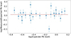 |
Fig. 1. log(CPN, obs/CPN) versus CPN for the 26 NV sources in the sample. The solid line indicates the mean log(CPN, obs/CPN). |
Although the solid line in Fig. 1 appears to agree with data rather well, the best-fit χ2 value of 63.2 for 25 d.o.f. indicates that the statistical quality of the fit is rather poor. However, this is mainly due to two sources where log(CPN, obs/CPN) is ∼3 − 4σ away from the mean. If we do not consider these objects, the agreement between CPN, obs and CPN is quite good (χ2 = 30.3/23 d.o.f., pnull = 0.14). We concluded that although CPN may not (always) provide an accurate measurement of the Poisson noise on an individual light curve basis, it gives a good estimate of CPN, obs on average. Since our work is based on the study of the average PSD of many sources in various groups (see next section), we adopted CPN, as defined by Eq. (2), as an estimate of the Poisson noise in the Swift/BAT light curves.
4.2. Computing and fitting the ensemble PSD of AGN
Although the periodogram is an unbiased estimator of the intrinsic PSD, its statistical properties are not ideal. The probability distribution of the periodogram estimates follows an χ2 distribution with two degrees of freedom, and their variance is large and unknown. In fact, the variance does not even decrease with increasing data points. For that reason, it is customary to smooth the periodogram using various ‘spectral windows’. However, smoothing in the linear space is not ideal in the case of power-law like intrinsic PSDs (PL93). An alternative option would be to bin the logarithmic periodogram as suggested by PL93, but that is not the best solution in our case either. Since jmax = 78, we would end up with just four points in the power spectrum over a limited frequency range if we followed the prescription of binning the log periodogram into groups of size M = 20. Fitting them with a straight line would result in best-fit parameters with large uncertainties. To avoid this, we followed a different approach to compute and fit the power spectra of the variable sources in the sample.
As we describe in the next section, we considered AGN in relatively small boxes in the log(LX) vs. log(MBH) plane (so that they have a similar BH mass and luminosity). Supposing there are nAGN in such a box (typically, nAGN = 4 − 6). We computed the periodogram of all AGN in each box, and we subtracted the Poisson noise level. We then computed the mean of the nAGN periodograms,  , at frequencies lower than 0.1 month−1, and we accepted log
![Mathematical equation: $ [\overline{I(\nu)}] $](/articles/aa/full_html/2024/05/aa47995-23/aa47995-23-eq10.gif) as an estimate of the ensemble mean power spectrum of the AGN in each [log(LX), log(MBH)] box. In a few cases,
as an estimate of the ensemble mean power spectrum of the AGN in each [log(LX), log(MBH)] box. In a few cases,  is negative at one or more frequencies. In such cases, we grouped these values together with the two
  in the adjacent frequencies, and we replaced all three mean periodograms with their mean.
At higher frequencies, the variance of the noise-subtracted power spectrum increases. In order to reduce the noise of the PSD at these frequencies, we further smoothed the mean  ’s using a simple top-hat window of size five, that is, we grouped every five successive
  ’s together, computed their mean, and accepted the logarithm as an estimate of the intrinsic PSD at the mean of the respective frequencies.
Since nAGN is small, the probability distribution of the resulting PSD estimates is not Gaussian, even at high frequencies. Therefore, we could not use traditional χ2 statistics to fit the observed power spectra. For that reason, we assumed that the intrinsic PSD follows a power-law like shape, and we fitted the power spectra with a line of the form in the log-log space:
 (3)
(3)
where PSDamp is the PSD amplitude at ν0 = 10−2 month−1. We chose this frequency to define the PSD amplitude because it is within the range of sampled frequencies, and it is reasonably low. Hence, the best-fit value would not be affected by aliasing (or other) effects (see the discussion below). We fitted the data following the ordinary least square (OLS) [Y|X] prescription of Isobe et al. (1990). In this way, even though we do not know the error of the logarithmic estimates of the power spectrum, we could still compute the best-fit line parameters, as well as their error.
As an example, Fig. 2 shows the average PSD of four AGN with log(MBH) ∼ 7 and log(LX) ∼43.5 (these are the objects that belong to the AGN group B4 in Fig. 4). The solid and dashed lines show the best-fit lines when we fit Eq. (3) to the PSD at frequencies below 0.1 months−1 and at all frequencies, respectively. The full-range best-fit slope is flatter than the low-frequency slope, with Δ(PSDslope)∼0.5. This is the PSD with one of the largest differences between the low- and the full frequency range best-fit slopes. Differences between the low-frequency and the full-range best-fit slopes appear in other power spectra as well, but they are smaller than 0.5 (see Table 1).
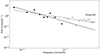 |
Fig. 2. Mean power spectrum of the AGN belonging to group B4, as indicated in Fig. 4. The power spectrum was computed as explained in Sect. 4. The solid and dashed lines show the best-fit lines when we fit the low-frequency and the full-range power spectrum (filled and filled+open circles, respectively). The model was defined by Eq. (3). |
Best-fit results for the power spectrum slope.
A PSD flattening may be due to the smoothing process at high frequencies, which may bias the observed power spectrum, and it may appear flatter than the intrinsic PSD. In addition, Swift/BAT does not observe all AGN continuously. In quite a few cases, the total exposure time in some bins is less than a day, which is much smaller than the bin size of the light curves. It is possible then that aliasing effects may be significant, in which case they will also flatten the observed PSDs at high frequencies. Such effects are difficult to model, as they depend on the intrinsic PSD and the actual observing pattern within each Δt. For that reason, we fitted the PSDs twice: once at frequencies below 10−1 month−1 (the LF fits, hereafter) and a second time over the full frequency range (the FR fits, hereafter).
5. Power spectrum analysis
5.1. The Sy1 and Sy2 PSDs
We first investigated whether the Sy1 and Sy2 power spectra are the same or not. The top panel in Fig. 3 shows a plot of log(LX) versus log(MBH) for all the variable sources in the sample. The black filled and red open circles indicate the Sy1 and the Sy2 sources, respectively. (Hereafter, we refer to both the Sy1.9 and Sy2 sources in the sample as ‘Sy2’.) On average, MBH in Sy2s appears to be larger when compared to Sy1s, while their intrinsic X-ray luminosity appears to be smaller. The investigation of the significance of these differences is outside the scope of our work; however, since the PSD may depend on MBH and/or LX we needed to compare the mean power spectrum of Sy1 and Sy2 with the same MBH and LX in order to test if they are similar or not.
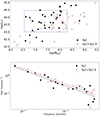 |
Fig. 3. Comparison between the Seyfert I and Seyfert II PSDs. Upper panel: Plot of log(LX), versus log(MBH) for the variable sources in the sample. Black and red circles indicate data for the Sy1 and Sy2 galaxies, respectively. The mean BH mass and LX of the Sy1 and Sy2 sources in the dashed box are similar. Lower panel: Mean PSD of all the Sy1 and Sy2 AGNs with similar luminosity and BH mass. Black and red points show the ensemble PSD of the Sy1 and Sy2 galaxies, which are in the dashed box drawn in the upper panel. Black and red dashed lines show the best-fit line to the PSDs. |
There are 23 Sy1s and 23 Sy2s in the box indicated by the dashed lines in the upper panel of Fig. 3. Their mean log(MBH) and log(LX) are consistent (within the errors):  , and 7.8 ± 0.1 for Sy1 and Sy2, while
  and 43.6 ± 0.1, respectively.
The lower panel in Fig. 3 shows the mean PSD of all the Sy1 and Sy2 AGNs within the same box (black filled, and red open circles, respectively). We fitted the power spectra with the model defined by Eq. (3). Black solid and red dashed lines show the best-fit lines to the full-range Sy1 and Sy2 PSDs, respectively. The LF(FR) best-fit line parameters are log(PSDamp, Sy1) = 0.36 ± 0.26(0.32 ± 0.28), log(PSDamp, Sy2) = 0.43 ± 0.31(0.40 ± 0.32), and PSDslope, Sy1 = −1.00 ± 0.07(−0.88 ± 0.09),PSDslope, Sy2 = −0.95 ± 0.05(−0.87 ± 0.09). Clearly, the Sy1 and Sy2 PSDs are consistent, within the errors. This result suggests that the variability properties of the Sy1 and Sy2 galaxies in the 14–195 keV band are identical. Given this result, we combined the light curves from Sy1 and Sy2 sources in order to investigate the dependence of the power spectrum on BH mass and/or luminosity.
5.2. The dependence of PSD slope on MBH, LX, and λEdd
It is not easy to model the periodogram of each individual AGN in our sample and investigate if and how it may depend on MBH and/or LX. Instead, we grouped the variable AGN into relatively narrow BH mass and luminosity bins, as indicated by the dashed lines in Fig. 4. Their size is small (Δlog(MBH) ∼Δlog(LX)∼0.5), so the MBH and LX of the AGN in each box should be within a factor of approximately two. Consequently, their ensemble PSD should provide a good estimate of the intrinsic PSD of an AGN with BH mass and X-ray luminosity equal to the mean MBH and LX of the objects in each box.
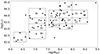 |
Fig. 4. log(LX), versus log(MBH) for the variable sources in the sample. The AGN within the boxes indicated by the dashed lines have similar MBH and LX. |
We computed the mean power spectrum of all AGN in each box (as explained in Sect. 4), and we fitted them with a line, as defined by Eq. (3). The best-fit slope should be indicative of the intrinsic slope of the AGN PSD. On the other hand, the best-fit amplitude may overestimate the intrinsic PSD amplitude because we have considered only the variable AGN in Fig. 4. This is appropriate when studying the PSD slope, as information on the slope can be provided only by sources with PSDs above the Poisson noise level. However, if there is a distribution of PSD amplitudes at each MBH,LX, then we should consider all AGN in each [MBH,LX] bin in order to measure the mean of the distribution, irrespective of whether they are variable or not (as long as they are at the same distance). We therefore used the best-fit slope from the model fits to the average PSDs of the variable AGN to study whether the PSDslope depends on MBH and/or LX; we discuss the dependence of PSDamp on these parameters in the next section. The best-fit results are listed in Table 1.
The top panel in Fig. 5 shows the LF best-fit PSD slope plotted as a function of the mean log(LX) for the AGN in groups B1, B2, B3 B4; C1, C2, C3; and D1, D2, D3, D4 (indicated with black circles, red circles, and brown squares, respectively). All the AGN in the B, C, and D groups have similar BH masses, with a mean of ∼7.1, 7.7, and 8.1, respectively (see Table 1). Within each of the B, C, and D groups, the PSD slope does not appear to depend on LX. The PSD slopes also appear to be similar between the various groups, which implies that the PSDslope does not depend on MBH either.
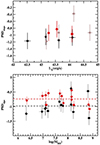 |
Fig. 5. Dependence of the PSD slope on X-ray luminosity and the BH mass. Upper panel: LF best-fit PSDslope plotted as function of log(LX) for the B, C, and D groups (black circles, red circles, and brown squares, respectively). Bottom panel: LF and FR PSDslope plotted as a function of |

To investigate these issues quantitatively, we fitted the data plotted in the top panel in Fig. 5 with a line of the form log(PSDslope) = a + b[log(LX)−43.5]. We took into account errors in both coordinates by using the fitexy routine of Press et al. (1992). We expected the PSDslope error to be similar when fitting the mean PSD in each bin, since the mean PSD is computed in the same way and the number of objects is roughly the same in all bins. The errors listed in Table 1 fluctuate mainly because of the small number of points in the PSDs (especially in the low-frequency part). The error on the slope turned out to be small in cases where the PSD points happened to align well around the best-fit line, while larger errors resulted in a case where the scatter of the points around the best-fit line is large (see also the discussion in Sect. IV in Isobe et al. (1990) on the best-fit errors in the case of a small number of data points). For that reason, we computed the mean error of all PSD slope estimates, and we assigned it to each PSDslope, assuming it is more representative of their intrinsic error.
The best-fit results from fitting the points in the top panel of Fig. 5 are bB = 0.06 ± 0.17, bC = −0.08 ± 0.19, and bD = 0.08 ± 0.14. All three best-fit b−values are consistent with zero, which shows that the PSDslope does not depend on LX. Furthermore, aB = −1.08 ± 0.16, aC = −0.92 ± 0.12, and aD = −0.98 ± 0.14. The best-fit a values for the various groups are also consistent with each other, which implies that the PSDslope does not depend on MBH either.
The bottom panel in Fig. 5 shows the best-fit PSD slope as a function of MBH for all groups shown in Fig. 4 and listed in Table 1. The black and red circles show the LF and FR PSD slopes, respectively. The mean LF and FR PSDslope is  and
and  . The black and red horizontal lines in the same panel indicate the mean LF and FR PSD slopes, respectively. When fitting the LF and FR data with these lines, we got χ2 = 18.2/13d.o.f. and 25.3/13 d.o.f., respectively. Both fits are statistically accepted (pnull = 0.15 and 0.02, respectively).
As a final test, we also investigated the possibility that the PSD slope may depend on the accretion rate. We fitted the LF and the FR PSD slopes versus log(λEdd) with a straight line of the form PSDslope[log(λEdd)] = aλEdd + bλEdd[log(λEdd)+1] (defined in this way, the normalization aλEdd is the PSD slope of a source with λEdd = −0.1). The fits were done taking into account the error on both variables. When considering the fit in the case of the LF slopes, the improvement in the goodness of fit is not significant (Δχ2 = 0.2 for 1 degree of freedom). However, in the case of the FR slopes, a straight line improves the fit significantly (Δχ2 = 9.3 for one extra degree of freedom; pnull = 0.002). This result implies that the PSD slope may depend on λEdd. The best-fit slope of the PSD slope versus λEdd relation is bλEdd, FR = 0.19 ± 0.06, which implies that the PSD slope may flatten with an increasing λEdd.
5.3. The dependence of PSD amplitude on MBH, LX, and λEdd
As we discussed in the previous section, we should consider all AGN in each [MBH,LX] bin in order to measure the intrinsic PSD amplitude, irrespective of whether they are variable or not, as long as they are at the same distance. Distance determines the S/N of the light curve for objects with the same luminosity. Even if the PSD amplitude is the same in two sources, if one of them is located farther away, the observed count rate will be small, and its observed PSD may not be above the Poisson noise. The apparent difference in the observed PSDs in this case will be due to differences in the distance of the sources and not in their PSD.
For that reason, we considered all AGN in the sample with a light curve with S/N ≥ 2. These objects are shown in Fig. 6. Just like in Fig. 4, the dashed lines in this figure indicate boxes with a small width so that all sources in each box should have similar MBH and LX. As before, we computed the mean power spectrum of all AGN in each box in Fig. 6 (explained in Sect. 4), and we fitted them with a line (as defined by Eq. (3)). The best-fit amplitude should be indicative of the (logarithm of the) intrinsic PSD amplitude in the AGN. The best-fit results are listed in Table 2.
Best-fit results for the power spectrum amplitude.
The top panel in Fig. 7 shows the LF best-fit log(PSDamp) plotted as a function of the mean log(LX) for the AGN in boxes B1′, B2′, B3′; C1′, C2′, C3′; and D1′, D2′, D3′, D4′ (black circles, red circles, and brown squares, respectively). We fitted the data with a line of the form log(PSDamp) = c + d[log(LX)−43.5]. The best-fit results are cB = −0.005 ± 0.08, cC = 0.09 ± 0.11, cD = 0.36 ± 0.22, and dB = −0.14 ± 0.20, dC = 0.28 ± 0.34, dD = −0.47 ± 0.32. The best-fit d values are all consistent with zero, indicating that the power spectrum amplitude does not depend on LX. The best-fit c values appear to increase when going from group B to group D, indicating an increase of PSDamp with increasing MBH. In reality, since c is equal to the PSD amplitude of an AGN with log(LX) = 43.5, such a dependence on MBH would imply that PSDamp increases with a decreasing accretion rate. However, formally speaking, the best-fit c values are consistent with each other(within 1.5σ), suggesting that this apparent dependence of log(PSdamp) on MBH is not significant.
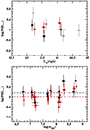 |
Fig. 7. Same as in Fig. 5 but for the PSD amplitude. The black, red, and brown points in the upper panel show the LF best-fit log(PSDamp) values plotted as a function of LX for AGN in the B′, C′, and D′ boxes in Fig. 6. The bottom panel shows all the LF and FR PSD amplitudes (listed in Table 2) plotted as a function of MBH (black and red points, respectively). The dashed lines indicate the respective mean PSD amplitudes. |
The bottom panel in Fig. 7 shows the best fit of the log(PSDamp) amplitude as a function of MBH for all the groups shown in Fig. 6 and listed in Table 2. The black and red circles show the LF and FR best-fit results, respectively. The black and red dashed lines indicate the LF and the FR mean logarithmic PSD amplitudes, respectively ( month−1, and
  month−1). These lines fit the data well (χ2 = 16.1/12 d.o.f. and χ2 = 14/12 d.o.f.).
We also investigated the possibility that the PSD amplitude may depend on the accretion rate. We therefore fitted the LF and the FR log(PSDamp) versus log(λEdd) data with a straight line of the form log(PSDamp)[log(λEdd)] = aλEdd + bλEdd[log(λEdd)+1]. The best fit results are bLF, λEdd = −0.30 ± 0.12 and bFR, λEdd = −0.26 ± 0.12. The improvement in the goodness of fit when we considered the straight line with a non-zero slope is significant in the case of the LF PSD amplitudes but less so in the case of the FR amplitudes: Δχ2 = 7.3 and 6.1 for one extra degree of freedom, respectively (pnull = 0.007 and 0.014). These results are indicative of an anti-correlation between the PSD amplitude and accretion rate (with the variability amplitude decreasing with increasing λEdd). This is consistent with the dependence of the best-fit c values on MBH that we mentioned above.
Our results so far show that the X-ray power spectrum in the 14–195 keV band is the same in all AGN: it has a power-law shape with the same average slope and amplitude irrespective of the BH mass and luminosity. This result holds irrespective of whether we consider the LF or the FR best-fit results. The mean PSD slope when we considered the LR and the FR results is different at the 3.9σ level:  . There is also a difference between the mean LF and FR PSD amplitude, but it is small and not significant:
  . We also found evidence that the PSD amplitude decreases with increasing λEdd.
5.4. Normalised excess variance analysis
We performed an excess variance analysis of the Swift/BAT light curves. The variance of a light curve is equal to the integral of the power spectrum from a low to a high frequency (e.g. Allevato et al. 2013). It can be measured relatively easily and can be used to verify the power spectrum results that we report in the previous section. However, the variance of a single light curve is a poor measurement of the intrinsic variance of the variable process, as Allevato et al. (2013) showed. We can nevertheless use the Swift/BAT light curves of the AGN in our sample to test the PSD analysis results as we describe below.
It is important that we compute the variance using light curves with the same duration in the rest frame of each source. The highest redshift in our sample is z = 0.105. The observed 157-month light curve of this source is 142 months long in its rest frame. We therefore removed points from all light curves until their rest-frame duration was 142 months (we removed points from the last part of the light curves), and we computed the normalised excess variance,  , using Eq. (1) in Allevato et al. (2013). We note that since the PSD slope is −1 (or even flatter), we did need to correct the variance estimates for bias (see Sect. 5 in Allevato et al. 2013). The normalized excess variance measurements for each source are listed in the ninth column of Table A.1.
Figure 8 shows a plot of  as a function of log(MBH) for all AGN plotted within the boxes drawn in Fig. 6. These are the objects we used to study the PSD amplitude. Therefore, we could test the PSD results we mentioned above using the
  measurements plotted in this figure. We first investigated whether the excess variance depends on MBH, LX, and/or λEdd by fitting the data with the following lines:
 ![Mathematical equation: $ {\sigma^2_{\rm NXV}}=a_{\rm BH}+b_{\rm BH}[\log(M_{\rm BH})-7.5] $](/articles/aa/full_html/2024/05/aa47995-23/aa47995-23-eq28.gif) ,
, ![Mathematical equation: $ {\sigma^2_{\rm NXV}}=a_{\rm Lx}+b_{\rm Lx}[\log(L_{\rm X})-43.5] $](/articles/aa/full_html/2024/05/aa47995-23/aa47995-23-eq29.gif) , and
, and ![Mathematical equation: $ {\sigma^2_{\rm NXV}}=a_{\lambda_{\rm Edd}}+b_{\lambda_{\rm Edd}}[\log(\lambda_{\rm Edd}+1)] $](/articles/aa/full_html/2024/05/aa47995-23/aa47995-23-eq30.gif) . All the best-fit bBH, bLx, and bλEdd values are consistent with zero, which indicates that
. All the best-fit bBH, bLx, and bλEdd values are consistent with zero, which indicates that  does not depend on MBH, LX, or λEdd. This is what we would expect if the PSD is the same in all AGN, irrespective of their BH mass, luminosity and/or accretion rate.
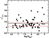 |
Fig. 8.
|

To test this hypothesis even further, we computed the mean excess variance of all AGN plotted in Fig. 8. We found  (indicated by the horizontal solid line in the same figure). If the excess variance is the same in all AGN, then
  should be an unbiased estimate, and its error should be a reliable estimate of the true error of the mean according to Allevato et al. (2013, see point 8 in their Sect. 8). Using Eq. (4) in Allevato et al. (2013) and the mean PSDamp and PSDslope we reported in the previous sections, we could predict the excess variance of light curves with Tmax = 142 days, and Tmin = 2Δt = (2months)/(1+
 ), where
  is the mean redshift of all AGN in the sample. The dashed lines in Fig. 8 indicate the expected excess variance in the case when we consider the LF PSD results (i.e. PSDslope ∼ −1 and log(PSDamp)∼0.15), while the dotted lines in the same figure indicate the expected excess variance in the case when we consider the FR PSD results (PSDslope ∼ −0.75 and log(PSDamp)∼0.01), taking into account the error on both log(PSDamp) and PSDslope. The model excess variance in both the LF and the FR cases are fully consistent with the observed
  .
.
We note that the results from the fit of a line to the FR PSDslope versus the λEdd data in Sect. 5.2 suggested that the PSDslope may depend on λEdd. If indeed the PSDslope ∝ 0.2[log(λEdd) + 1], as we found, then we would expect the AGN excess variance to increase with λEdd and bλEdd, FR = 0.05. We found bλEdd, FR = −0.06 ± 0.035, that is, the opposite trend. The difference between the predicted and the observed bλEdd, FR is at the 3σ level. We concluded that it is rather unlikely that the intrinsic PSD slope depends on λEdd. On the other hand, in the last paragraph of the previous section, we noticed a trend of decreasing PSD amplitude with increasing λEdd. Assuming the LF best-fit results, we would predict that  should also decrease with increasing λEdd, with bλEdd, SR = −0.06, exactly as observed: bλEdd, obs = −0.06 ± 0.04. This result further suggests that the PSD amplitude indeed decreases with an increasing accretion rate.
6. Summary and discussion
We used 157-month Swift/BAT light curves to compute the mean X-ray PSD of the brightest AGN in the BASS survey, using various BH mass and X-ray luminosity bins that span two orders of magnitude in BH mass (6.5 ≲ log(MBH)≲8.5) and X-ray luminosity (42.5 ≲ log(LX)≲44.5; see Tables 1 and 2). As we have mentioned, the AGN in our sample should be representative of the radio-quiet AGN population in the local universe. We fitted the average power spectra with a power-law model of the form  (where ν0 = 0.01 month−1). Our results are summarised below:
(1) The mean X-ray PSD of AGN (in the 4–195 keV band) at low frequencies (∼6.5 × 10⁻³ − 0.5 month−1) is consistent with the power-law model. We did not detect periodicities or quasi-periodic oscillations, nor did we detect any ‘bending’ frequencies within the sampled frequency range, where the PSD slope would steepen (at higher frequencies) or flatten (at lower frequencies).
(2) The X-ray power spectrum of Seyfert I and Seyfert II galaxies are consistent with each other (within errors). This result shows that the X-ray variability mechanism is consistent with being the same in both classes of AGN. This is in agreement with the AGN unification model.
(3) The mean log(PSDamp), which is defined as the PSD value at ν0 = 0.01/month, is 0.15 ± 0.06(0.01 ± 0.07) month−1 based on the LF(FR) PSD best-fit results. We expected a distribution of log(PSDamp) values in AGN with a given BH mass and X-ray luminosity. Our results show that the mean of the logarithm of the PSD amplitude distributions should be ∼0.015 month−1 in all the AGN, irrespective of their MBH and/or LX.
(4) We found significant evidence that the PSD amplitude of the individual AGN should decrease with an increasing accretion rate as follows: PSDamp(λEdd)∝(λEdd/0.1)−0.3. This result implies that the variability amplitude in AGN should decrease with an increasing accretion rate.
(5) Just as with the PSD amplitude, our results indicate that the mean PSD slope should also be the same in all AGN, irrespective of their BH mass or luminosity. The average PSD slope is −0.98 ± 0.06 when fitting only the LF PSD, and it becomes −0.74 ± 0.04 when we fit the full range of PSDs. We believe that the slope flattening when we consider high frequencies as well may be due (mainly) to aliasing effects. We also detected a significant dependence of the PSD slope on λEdd when we considered the full range of results. The power spectrum slope appears to flatten with increasing λEdd. As we discuss below, this result is also due to aliasing effects, and it does not imply an intrinsic dependence of the PSD slope on the accretion rate.
(6) The normalised excess variance,  , does not depend on BH mass or LX. This result is consistent with the PSD results. If the average X-ray PSD is the same in all AGN, then its integral,
  , should be independent of the AGN parameters, just as we observed.
6.1. The universal shape of the mean X-ray PSD of AGN
Our results suggest that, on average, the X-ray PSD (in the 14–195 keV band) should be the same in all AGN. If that is the case, then we can compute the mean AGN PSD if we use the periodograms of all the variable sources in our sample. To this end, we computed the mean PSD of all variable AGN in our sample (corrected from the Poisson noise) as explained in Sect. 4. The resulting mean PSD is shown in Fig. 9. We have smoothed the high frequency PSD points (above 0.1 month−1), as explained in the same section.
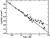 |
Fig. 9. Mean PSD of the variable AGN in our sample. The solid line shows the best-fit power-law model for the data up to 10−7.4 Hz, and the dashed line shows the same model with aliasing effects included (see Sect. 6.1 for details). |
The mean PSD is fully consistent with a simple power-law model. The solid line in this figure shows the best-fit model when we fit the data below 10−7.4 Hz (=0.1/month) with a power-law model defined by Eq. (3). This line provides a very good fit to the LF part of the PSD (χ2 = 10.6/13 d.o.f.), with a best-fit slope of −1.00 ± 0.06. The PSD amplitude is larger than the mean amplitude we report in Sect. 5.3, but that is because here we considered only the variable AGN (in order to determine the PSD slope correctly).
The fact that a −1 power-law model fits the LF part of the mean PSD so well strongly supports the hypothesis that there is no PSD flattening, even at frequencies as low as ∼3 × 10⁻⁹ Hz. For example, if there was a low-frequency flattening for low-mass BHs in our sample, we would expect the lowest frequency points in the mean PSD to show a much larger scatter when compared to the higher frequency points, but that is not the case. We believe that our results clearly show that the average AGN PSD follows a power-law shape with a slope of −1 down to frequencies as low as a few 10−9 Hz (this frequency corresponds to a timescale of ∼12 years).
The mean PSD flattens at frequencies higher than ∼4 × 10⁻⁸ Hz. We do not believe that this is due to a systematic bias in the computation of the Poisson noise level (see Fig. 1 and the discussion in Sect. 4.1). As we discussed in Sect. 4.2, the high frequency flattening could be due to aliasing effects. The dashed line in Fig. 9 shows the best-fit power-law model (the one plotted with the solid line) when we also include the aliasing effects in the case when the PL extends to 2 × 10⁻⁶ Hz and the light curve is evenly sampled. The frequency of 2 × 10⁻⁶ Hz indicates the high-frequency break in the 2–10 keV PSD of an AGN with log(MBH) = 7.5, according to the model defined by Eq. (4) in González-Martín & Vaughan (2012). The agreement between the dashed line and the mean PSD at high frequencies is quite good. This result supports the fact that the PSD flattening we detect at high frequencies is probably due to aliasing effects.
Support to the hypothesis of aliasing affecting the measured PSD slope when we consider the full frequency range is also provided by the apparent dependence of the PSD slope on λEdd when we consider the FR results (see Sect. 5.2). According to McHardy et al. (2006), the PSD bending frequency should increase with increasing λEdd. In this case, we would also expect the aliasing effects to become stronger, thus resulting in a flattening of the PSD slope with increasing λEdd, as observed.
The hard X-ray PSD should steepen above a bending frequency, νb, just as in the 2–10 keV band. The fact that such a bending must exist, and is probably located at a frequency similar to the high-frequency break in the 2–10 keV PSDs, is supported by the agreement of the dashed line and the mean PSD in Fig. 9. If the intrinsic hard X-ray PSD would extend to very high frequencies without bending to a slope steeper than −1, then irrespective of the sampling pattern of the Swift/BAT light curves, the aliasing effects would be much stronger, and the high-frequency flattening in Fig. 9 would be much more pronounced. If the bending frequency does not vary significantly with energy, we would then expect νb ∼ 470 − 4.7 month−1 (i.e. ∼1.8 × 10⁻⁴ − 1.8 × 10⁻⁶ Hz) for AGN with log(MBH) = 6.5–8.5 (which is the majority of the AGN in our sample). These frequencies cannot be sampled with the current Swift/BAT light curves. NuSTAR light curves would be necessary in order to detect and investigate the bending frequency properties at hard X-rays.
If the bending frequency does not depend significantly on energy, this would imply that the hard X-ray PSD in AGN extends with a slope of −1 over ∼2.8 − 4.8 decades for AGN with log(MBH) = 8.5-6.5, respectively. This is a large frequency range, and this result would have interesting implications, at least for AGN with BH masses smaller than a few 107 M⊙. For example, the Ark 564 PSD shows a significant low-frequency break to slope zero at ∼10−6 Hz, approximately three orders of magnitude below the high-frequency break (McHardy et al. 2007; Papadakis et al. 2002). This is the only AGN where such a low-frequency flattening has been detected in its X-ray PSD. It is quite possible then that such PSDs are not very common in AGN. As we argued above, if this were common, we would expect the low-frequency points in the PSD plotted in Fig. 9 to show evidence of a low-frequency flattening and to be very noisy.
6.2. Comparison with past results
Table 3 in SM13 lists the authors’ best-fit log(PSDamp) and PSDslope results when they fit an unbroken power-law model to the data. We fit the same model to the Swift/BAT power spectra. According to the SM13 results, the PSD at ν0 = 0.01 month−1 should be given by PSDSM13(ν0) = ASM13(ν0/νSM13)−PSDslope, SM13, where νSM13 = 10−6 Hz, and it should be consistent with the amplitude of our PSD model. Using the SM13 best-fit results, we found ![Mathematical equation: $ \overline{\log[\mathrm{PSD}_{\mathrm{SM13}}(\nu_0)]}=-0.13\pm 0.10 $](/articles/aa/full_html/2024/05/aa47995-23/aa47995-23-eq42.gif) , which is entirely consistent with our LF mean log(PSDamp) measurement.
, which is entirely consistent with our LF mean log(PSDamp) measurement.
Furthermore, the authors of SM13 found a mean PSD slope of −0.78 ± 0.29, which became −0.92 ± 0.22 when they restricted the average to only the 16 best-fit slopes that were fully constrained (out of the 30 sources in their sample). The results of SM13 are very similar to ours. We found a mean slope of ∼ − 0.75 when we fitted the full-range PSDs and a steeper slope of ∼ − 1 when we considered only the LF part of the power spectrum. As we mentioned above, we believe that the −1 value is probably more representative of the intrinsic PSD slope mainly because aliasing effects may flatten the PSD at high frequencies. Such effects should not be important in the SM13 power spectra because the authors used light curves with a bin size of one day. Since the power at frequencies higher than ∼1 day should be significantly smaller than the power at low frequencies, aliasing effects should not be important in this case. On the other hand, as the authors of SM13 commented, their best-fit PSD slopes are well constrained only when the power spectra are well above the Poisson noise. The fact that the mean slope in this case is closer to our mean in the case of the LF best-fit results reinforces our belief that −1 is probably closer to the intrinsic PSD slope of the AGN X-ray PSD at low frequencies.
6.3. Comparison with the 2–10 keV band PSD results
As we have already mentioned in the introduction, many works in the past have shown that the low-frequency PSD of AGN at energies below 10 keV has a slope of −1. As we discussed in Sect. 6.1, this is probably the case of the low-frequency hard X-ray PSD in AGN as well. Therefore, our results suggest that the slope of the low-frequency PSD in the AGN does not depend on energy. This is contrary to what is observed at high frequencies in the 2–10 keV band PSD, where the slope above the high-frequency break appears to flatten with energy.
Our results are in agreement with the results of Paolillo et al. (2023), who found that over a large range of BH mass and luminosity, the 2–10 keV PSD has the same shape in all AGN. Both in the 2–10 keV band and in the 14–195 keV band, the universal PSD slope at low frequencies is consistent with −1. On the other hand, Paolillo et al. (2023) found that PSD2 − 10 keV(νb)×νb = 0.008 ± 0.002, which is smaller than our estimate of 0.014 ± 0.003. This could imply that the PSD amplitude is larger at higher energies, although the difference is not statistically significant.
Excess variance studies in the 2–10 keV band indicate that  (Ponti et al. 2012; Paolillo et al. 2017). If this holds in the 14–195 keV band as well, it would imply a similar dependence of PSDamp on λEdd. We did detect a significant anti-correlation between PSD amplitude and λEdd in our data (see Sect. 5.3). We found that PSDamp ∝ (λEdd)−0.30 ± 0.12, which is flatter than the anti-correlation that the 2–10 keV data imply (although the 2–10 keV relation is not well defined and no error is given on the slope). Perhaps the PSD amplitude-λEdd anti-correlation at energies higher than 15 keV is not as steep as the one at lower energies, although a more detailed study of this effect in the 2–10 keV band is necessary to understand if there are differences between the two bands.
6.4. Comparison with the GBH PSD
Active galactic nuclei and GBHs are both powered by the accretion of matter on BHs, but a major difference is the mass of the BH at their centre. It has long been suggested that the X-ray variability mechanism is the same in both systems. However, the PSD of GBHs depends on the ‘state’ of the system. There are two main states in GBHs: hard and soft. The PSD in the soft state is usually well described by a single bending power-law, with a slope equal to or steeper than −2 above νb and a slope of −1 extending to very low frequencies. In the hard state, the PSD is more complex and is usually modelled as a mixture of zero-centred Lorentzian components. It is true that similar power spectra from the hardest part of the hard state show a shape similar to the soft state PSDs (e.g. Heil et al. 2015). In general, however, black hole X-ray binary hard states show power spectra with slopes ∼ − 1 over at least one to two decades in frequency, which bend to a constant (i.e. to a slope of zero) at lower frequencies (e.g. Remillard & McClintock 2006). Based on the shape of the AGN PSDs (e.g. McHardy et al. 2004; Markowitz et al. 2003; Uttley & McHardy 2005; see also Paolillo et al. 2023) as well as the scaling of the −1 to −2 bending frequencies between AGN and GBHs (McHardy et al. 2006), it has been argued that almost all of X-ray bright AGN should be the analogues of the GBHs in their soft state. The authors of SM13 reached the same conclusion because they did not find any evidence for a low-frequency break to a slope of zero in the AGN Swift/BAT PSDs they studied.
We compared our results with the results from the PSD analysis of Cyg X-1 light curves when the source is in the soft state. Such a comparison between the timing properties of AGN and Cyg X-1 in its soft state has been done many times in the past (e.g. Uttley et al. 2002; McHardy et al. 2006). The solid grey lines in Fig. 10 show the Cyg X-1 PSDs (in PSD(ν)×ν representation) when the source is in its soft state. The data are from Axelsson et al. (2006), who analysed all the archival Cyg X-1 data from the Rossi X-ray Timing Explorer (RXTE) from 1996 to 2003 in the 2–9 keV band and in the frequency range of 0.01–25 Hz. They used various models to fit the PSDs, and one of them was a cut-off power-law (their Eq. (2)). The grey lines in the figure show the best-fit models when the PSDs were fitted only by the cut-off power law. According to the authors, this model fits the PSD well only when the source is in its canonical soft state. Figure 10 shows that the amplitude of the Cyg X-1 PSD in the soft state varies by a factor ∼15 or so. The PSD amplitude probably varies among AGN as well, as we have discussed above, but what is of interest is comparing the mean AGN PSD with the mean Cyg X-1 PSD in its soft state.
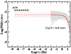 |
Fig. 10. Comparison between the mean AGN power spectrum and the Cyg X-1 PSD in its soft state. The grey lines show the Cyg X-1 PSDs in their canonical soft state according to Axelsson et al. (2006). The solid red line indicates their mean, while the red dashed and dotted lines show their extension and 1σ scatter, respectively, to lower frequencies. The solid black and brown lines indicate the mean AGN PSD when we consider our LF and FR best-fit results, respectively. The dashed lines indicate the 1σ scatter due to the PSDamp error. |
The solid red line in Fig. 10 shows the mean Cyg X-1 PSD. The dashed line shows its extension to lower frequencies, while the dotted lines indicate the 1σ spread of the PSD normalisation around its mean. The solid black line shows the mean best-fit PSD of the AGN in our sample. The frequency range extends to 10−6 Hz, as SM13 showed the AGN PSDs extend as a power-law up to that frequency. The dashed lines indicate the 1σ uncertainty of the best-fit to the mean PSDamp. Clearly, the mean AGN PSD agrees very well with the Cyg X-1 PSD in its soft state. The difference in BH mass between the AGN in our sample and Cyg X-1 is ∼106 − 108, while the difference in frequency between the Cyg X-1 and AGN PSDs is over four to five orders of magnitude. Despite these differences the PSD slopes are identical, and the mean PSD amplitudes differ only by a factor of three, maximum. We suspect that this difference is probably due to the difference in energy bands (2–9 KeV for Cyg X-1, as opposed to 14–195 keV for AGN). We plan to investigate this issue further in the near future.
We note that the agreement between the mean AGN PSD and the Cyg X-1 PSD in its soft state is quite plausible but, strictly speaking, only suggestive at this point. For example, hard-state low-frequency breaks can be seen from 0.01 Hz and higher, which would be 10−9 Hz or higher for a 108 M⊙ mass BH, assuming linear mass-scaling. As we discussed in Sect. 6.1, if that were the case, we would have detected it in the mean AGN PSD. However, we cannot be certain about the location of the high-frequency breaks in these objects (at the hard X-ray PSD). If the mean AGN PSD are similar to the GBH PSD in the hard state, then the −1 to −2 breaks in AGN at energies higher than 15 keV must be located at frequencies much lower than the ones we have detected at energies below 10 keV.
On the other hand, if the mean AGN PSD is like the mean Cyg X-1 in its soft state, then it is possible that the physical properties are similar in both systems. It is generally believed that the accretion disc extends to its innermost radius, and the X-ray corona is less luminous than the disc in GBHs when in their soft state. This could then be the case in AGN as well. The disc should extend to its innermost radius, and its emission would dominate the output in these objects as well (as is indeed the case with the ‘big blue bump’ that is observed in these objects). Given the inner disc radius, the corona cannot be located within the disc, and it has to be located on top of it (or above the central BH), illuminating the disc and causing all the X-ray reflection features (i.e. soft excess, broad iron line, and Compton hump) as well as the X-ray reverberation phenomena (e.g. driving the UV-optical variability and producing the delays between X-rays and UV-optical variations).
The count rate error in the Swift-BAT light curves is inversely proportional to the square root of the exposure time in each bin (this is easily checked when plotting errors versus the respective exposure time), and it does not depend on the source’s flux. In this case, the weighted rather than the straight mean is more representative of the source’s mean flux.
We computed the mean of log[IN(fj)] instead of the mean of IN(fj) because the error of the latter is known and is equal to  (PL93).
Acknowledgments
We would like to thank the referee for their comments which helped us improve the original version of the paper.
References
- Allevato, V., Paolillo, M., Papadakis, I., & Pinto, C. 2013, ApJ, 771, 9 [NASA ADS] [CrossRef] [Google Scholar]
- Axelsson, M., Borgonovo, L., & Larsson, S. 2006, A&A, 452, 975 [NASA ADS] [CrossRef] [EDP Sciences] [Google Scholar]
- Baumgartner, W. H., Tueller, J., Markwardt, C. B., et al. 2013, ApJS, 207, 19 [Google Scholar]
- Beckmann, V., Barthelmy, S. D., Courvoisier, T. J. L., et al. 2007, A&A, 475, 827 [NASA ADS] [CrossRef] [EDP Sciences] [Google Scholar]
- Beckmann, V., Soldi, S., Ricci, C., et al. 2009, A&A, 505, 417 [NASA ADS] [CrossRef] [EDP Sciences] [Google Scholar]
- Caballero-Garcia, M. D., Papadakis, I. E., Nicastro, F., & Ajello, M. 2012, A&A, 537, A87 [NASA ADS] [CrossRef] [EDP Sciences] [Google Scholar]
- González-Martín, O., & Vaughan, S. 2012, A&A, 544, A80 [NASA ADS] [CrossRef] [EDP Sciences] [Google Scholar]
- Green, A. R., McHardy, I. M., & Lehto, H. J. 1993, MNRAS, 265, 664 [NASA ADS] [Google Scholar]
- Heil, L. M., Uttley, P., & Klein-Wolt, M. 2015, MNRAS, 448, 3339 [NASA ADS] [CrossRef] [Google Scholar]
- Isobe, T., Feigelson, E. D., Akritas, M. G., & Babu, G. J. 1990, ApJ, 364, 104 [Google Scholar]
- Koss, M. J., Ricci, C., Trakhtenbrot, B., et al. 2022, ApJS, 261, 2 [NASA ADS] [CrossRef] [Google Scholar]
- Lawrence, A., & Papadakis, I. 1993, ApJ, 414, L85 [NASA ADS] [CrossRef] [Google Scholar]
- Lusso, E., Comastri, A., Simmons, B. D., et al. 2012, MNRAS, 425, 623 [Google Scholar]
- Markowitz, A. 2010, ApJ, 724, 26 [NASA ADS] [CrossRef] [Google Scholar]
- Markowitz, A., Edelson, R., Vaughan, S., et al. 2003, ApJ, 593, 96 [NASA ADS] [CrossRef] [Google Scholar]
- Markowitz, A., Papadakis, I., Arévalo, P., et al. 2007, ApJ, 656, 116 [CrossRef] [Google Scholar]
- McHardy, I. M., Papadakis, I. E., Uttley, P., Page, M. J., & Mason, K. O. 2004, MNRAS, 348, 783 [NASA ADS] [CrossRef] [Google Scholar]
- McHardy, I. M., Koerding, E., Knigge, C., Uttley, P., & Fender, R. P. 2006, Nature, 444, 730 [NASA ADS] [CrossRef] [Google Scholar]
- McHardy, I. M., Arévalo, P., Uttley, P., et al. 2007, MNRAS, 382, 985 [Google Scholar]
- Oh, K., Koss, M., Markwardt, C. B., et al. 2018, ApJS, 235, 4 [Google Scholar]
- Paolillo, M., Papadakis, I., Brandt, W. N., et al. 2017, MNRAS, 471, 4398 [Google Scholar]
- Paolillo, M., Papadakis, I. E., Brandt, W. N., et al. 2023, A&A, 673, A68 [NASA ADS] [CrossRef] [EDP Sciences] [Google Scholar]
- Papadakis, I. E., & Lawrence, A. 1993, MNRAS, 261, 612 [Google Scholar]
- Papadakis, I. E., Brinkmann, W., Negoro, H., & Gliozzi, M. 2002, A&A, 382, L1 [NASA ADS] [CrossRef] [EDP Sciences] [Google Scholar]
- Ponti, G., Papadakis, I., Bianchi, S., et al. 2012, A&A, 542, A83 [NASA ADS] [CrossRef] [EDP Sciences] [Google Scholar]
- Press, W. H., Teukolsky, S. A., Vetterling, W. T., & Flannery, B. P. 1992, Numerical Recipes in FORTRAN. The Art of Scientific Computing (Cambridge University Press) [Google Scholar]
- Remillard, R. A., & McClintock, J. E. 2006, ARA&A, 44, 49 [Google Scholar]
- Shimizu, T. T., & Mushotzky, R. F. 2013, ApJ, 770, 60 [NASA ADS] [CrossRef] [Google Scholar]
- Soldi, S., Beckmann, V., Baumgartner, W. H., et al. 2014, A&A, 563, A57 [NASA ADS] [CrossRef] [EDP Sciences] [Google Scholar]
- Uttley, P., & McHardy, I. M. 2005, MNRAS, 363, 586 [NASA ADS] [CrossRef] [Google Scholar]
- Uttley, P., McHardy, I. M., & Papadakis, I. E. 2002, MNRAS, 332, 231 [Google Scholar]
- Vaughan, S. 2005, A&A, 431, 391 [NASA ADS] [CrossRef] [EDP Sciences] [Google Scholar]
Appendix A: Appendix
Active galactic nuclei in the sample and their properties.
All Tables
All Figures
|
Fig. 1. log(CPN, obs/CPN) versus CPN for the 26 NV sources in the sample. The solid line indicates the mean log(CPN, obs/CPN). |
| In the text | |
|
Fig. 2. Mean power spectrum of the AGN belonging to group B4, as indicated in Fig. 4. The power spectrum was computed as explained in Sect. 4. The solid and dashed lines show the best-fit lines when we fit the low-frequency and the full-range power spectrum (filled and filled+open circles, respectively). The model was defined by Eq. (3). |
| In the text | |
|
Fig. 3. Comparison between the Seyfert I and Seyfert II PSDs. Upper panel: Plot of log(LX), versus log(MBH) for the variable sources in the sample. Black and red circles indicate data for the Sy1 and Sy2 galaxies, respectively. The mean BH mass and LX of the Sy1 and Sy2 sources in the dashed box are similar. Lower panel: Mean PSD of all the Sy1 and Sy2 AGNs with similar luminosity and BH mass. Black and red points show the ensemble PSD of the Sy1 and Sy2 galaxies, which are in the dashed box drawn in the upper panel. Black and red dashed lines show the best-fit line to the PSDs. |
| In the text | |
|
Fig. 4. log(LX), versus log(MBH) for the variable sources in the sample. The AGN within the boxes indicated by the dashed lines have similar MBH and LX. |
| In the text | |
|
Fig. 5. Dependence of the PSD slope on X-ray luminosity and the BH mass. Upper panel: LF best-fit PSDslope plotted as function of log(LX) for the B, C, and D groups (black circles, red circles, and brown squares, respectively). Bottom panel: LF and FR PSDslope plotted as a function of |
| In the text | |
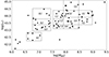 |
Fig. 6. Same as in Fig. 4 for all AGN in the sample with a light curve with S/N ≥ 2. |
| In the text | |
|
Fig. 7. Same as in Fig. 5 but for the PSD amplitude. The black, red, and brown points in the upper panel show the LF best-fit log(PSDamp) values plotted as a function of LX for AGN in the B′, C′, and D′ boxes in Fig. 6. The bottom panel shows all the LF and FR PSD amplitudes (listed in Table 2) plotted as a function of MBH (black and red points, respectively). The dashed lines indicate the respective mean PSD amplitudes. |
| In the text | |
|
Fig. 8.
|
| In the text | |
|
Fig. 9. Mean PSD of the variable AGN in our sample. The solid line shows the best-fit power-law model for the data up to 10−7.4 Hz, and the dashed line shows the same model with aliasing effects included (see Sect. 6.1 for details). |
| In the text | |
|
Fig. 10. Comparison between the mean AGN power spectrum and the Cyg X-1 PSD in its soft state. The grey lines show the Cyg X-1 PSDs in their canonical soft state according to Axelsson et al. (2006). The solid red line indicates their mean, while the red dashed and dotted lines show their extension and 1σ scatter, respectively, to lower frequencies. The solid black and brown lines indicate the mean AGN PSD when we consider our LF and FR best-fit results, respectively. The dashed lines indicate the 1σ scatter due to the PSDamp error. |
| In the text | |
Current usage metrics show cumulative count of Article Views (full-text article views including HTML views, PDF and ePub downloads, according to the available data) and Abstracts Views on Vision4Press platform.
Data correspond to usage on the plateform after 2015. The current usage metrics is available 48-96 hours after online publication and is updated daily on week days.
Initial download of the metrics may take a while.