| Issue |
A&A
Volume 698, June 2025
|
|
|---|---|---|
| Article Number | A105 | |
| Number of page(s) | 21 | |
| Section | Extragalactic astronomy | |
| DOI | https://doi.org/10.1051/0004-6361/202452469 | |
| Published online | 03 June 2025 | |
High-frequency breaks in the optical active galactic nucleus power spectral density
Homer L. Dodge Department of Physics and Astronomy, University of Oklahoma, 440 W. Brooks St., Norman, OK 73019, USA
⋆ Corresponding author.
Received:
2
October
2024
Accepted:
24
March
2025
Abstract
Context. Variability is a ubiquitous feature of active galactic nuclei (AGNs), and the characterisation of this variability is crucial to constraining its physical mechanism and proper applications in AGN studies. The advent of all-sky and high-cadence optical surveys allows more accurate measurements of AGN variability down to short timescales as well as direct comparisons with X-ray variability from the same sample of sources.
Aims. We aim to analyse the optical power spectral density (PSD) of AGNs with measured X-ray PSDs.
Methods. We used light curves from the All-Sky Automated Survey for SuperNovae (ASAS-SN) and the Transiting Exoplanet Survey Satellite (TESS) and used the Lomb-Scargle periodogram to obtain PSDs. The joint optical PSD is measured over up to six orders of magnitude in frequency space on timescales of minutes to a decade. We fitted either a damped random walk (DRW) or a broken power law (BPL) model to constrain the PSD model and break frequency.
Results. We find a set of break frequencies (≲10−2 day−1) from DRW and BPL fits that generally confirm previously reported correlations between break frequencies and the black hole mass. In addition, we find a second set of break frequencies at higher frequencies (> 10−2 day−1). We observe a potential weak correlation between the high-frequency breaks with the X-ray break frequencies and the black hole mass. We further explored the dependence of the correlations on other AGN parameters, finding that adding X-ray, optical, or bolometric luminosity as the third correlation parameter can substantially improve the correlation significances. The newly identified high-frequency optical breaks can constrain different aspects of the physics of AGNs.
Key words: galaxies: active
© The Authors 2025
 Open Access article, published by EDP Sciences, under the terms of the Creative Commons Attribution License (https://creativecommons.org/licenses/by/4.0), which permits unrestricted use, distribution, and reproduction in any medium, provided the original work is properly cited.
This article is published in open access under the Subscribe to Open model. This email address is being protected from spambots. You need JavaScript enabled to view it. to support open access publication.
1. Introduction
Variability is a ubiquitous characteristic of active galactic nuclei (AGNs), and is observed at all wavelengths (e.g. Mushotzky et al. 1993; Vanden Berk et al. 2004) and on all timescales (e.g. Grandi et al. 1992; Markowitz et al. 2003). The mechanism driving the variability is still debated. A number of theories have been suggested, such as accretion disc instabilities (e.g. Kawaguchi et al. 1998; Trèvese & Vagnetti 2002), global inhomogeneities from infall or thermal processes (e.g. Lightman & Eardley 1974; Shakura & Sunyaev 1976; Kelly et al. 2009), local disc communication processes on sound crossing or Alfvén timescales (Dexter & Agol 2011), magnetorotational instabilities (e.g. Balbus & Hawley 1991; Reynolds & Miller 2009), and reprocessing between the disc and the corona on light crossing timescales (e.g. Haardt & Maraschi 1991; McHardy et al. 2018).
Though its origin is uncertain, AGN variability provides clues about the physical properties of the central engine. The variability at different wavelengths is known to arise from different regions of the AGN, and the variability time lags in different wavelengths can be used for reverberation mapping to measure the physical size of the AGN structure and the mass of the central supermassive black hole (SMBH; e.g. Wandel et al. 1999; Kaspi et al. 2000; Peterson et al. 2005). Different classes of AGNs also show different variability features (e.g. Ptak et al. 1998), and by studying these differences, we can learn specific details about each class. As a behaviour common to all AGNs, variability can also be used to find AGNs (e.g. Butler & Bloom 2011; MacLeod et al. 2011; Ruan et al. 2012; Treiber et al. 2022; Yuk et al. 2022).
The stochastic variability of AGNs can be characterised by its power spectral density (PSD). PSDs are characterised by red noise, where the power increases for lower frequencies and then saturates below some frequency (e.g. Uttley et al. 2002). For optical variability this is commonly modelled as a damped random walk (DRW; e.g. Kelly et al. 2009; Kozłowski 2016). In these models, the DRW break frequency, the frequency where the PSD starts to flatten, is correlated with the mass of the SMBH powering the AGN (e.g. Kelly et al. 2009; MacLeod et al. 2010; Burke et al. 2021). With the recent advent of high-cadence optical data, we can now probe the optical PSD on short timescales (e.g. Smith et al. 2018), where steeper power law slopes than −2, the slope from the DRW model, were inferred (Mushotzky et al. 2011).
The X-ray variability of AGNs has been observed down to very short timescales (< 1 day; e.g. Grandi et al. 1992; Uttley et al. 2002), and many PSD and break frequency studies have been conducted (e.g. Uttley et al. 2002; McHardy et al. 2004; González-Martín & Vaughan 2012; González-Martín 2018; Smith et al. 2018). However, previous studies were limited by the differences in optical and X-ray timing surveys, and direct comparisons betweens optical and X-ray PSDs for the same set of sources were difficult. For this study, we combined the long-term, low-cadence, ground-based data from the All-Sky Automated Survey for SuperNovae (ASAS-SN; Shappee et al. 2014a; Kochanek et al. 2017) and the short-term, high-cadence, space-based data from the Transiting Exoplanet Survey Satellite (TESS; Ricker et al. 2015). We constructed a PSD separately for each dataset and then merged them to identify the break frequencies. This allowed the first systematic comparison of optical and X-ray break frequencies in the power spectra of AGNs. For this comparison, we used the sample of AGNs with X-ray break frequencies measured by González-Martín (2018). We introduce the sample, the ASAS-SN and TESS data, and the data analysis procedure in Section 2. We describe the methods for extracting and fitting the PSDs in Section 3. In Section 4, we present the resulting break frequencies and examine how they relate to previous results. We discuss the implications in Section 5.
2. Data
2.1. Data properties and the sample
ASAS-SN (Shappee et al. 2014a; Kochanek et al. 2017) began surveying the sky in 2012. After several expansions, it now consists of 20 14-cm telescopes distributed over five ‘units’ and can cover the visible sky nightly in good conditions. The two original units initially used the V-band filter. The three new units commissioned in 2017 use g-band filters and the original two units switched to the g band in 2018. During the transition, there were approximately 400 days when both the V band and the g band were used. ASAS-SN images have limiting magnitudes of V ∼ 16.5 − 17.5 and g ∼ 17.5 − 18.5 depending on lunation, a field of view of 4.5 deg2, a pixel scale of  , and a typical full width half maximum (FWHM) of ∼2 pixels.
Launched in 2018, TESS (Ricker et al. 2015) is equipped with four cameras and its TESS bandpass spans a wavelength range of 600 to 1000 nm. Each camera has a field of view of 24° by 24°. The combined 24° by 96° field of view is called a sector. TESS observes each sector for approximately 27.4 days. For the primary mission, the 26 sectors observed until July 2020, the full-frame images (FFIs) were taken with a 30-minute cadence. The first extended mission, which lasted until sector 55 in September 2022, collected FFIs with a 10-minute cadence. In the current, second extended mission, the FFIs are taken with a 200-second cadence. Each sector is divided into two cycles, each lasting for approximately 13 days, with ∼1 day gap in between for data transmission. The FFIs have the pixel scale of  with a typical FWHM of ∼2 pixels. The FFIs used for this study can be found in Mikulski Archive for Space Telescopes (MAST1).
González-Martín (2018) provided the most recent compilation of AGNs with measured X-ray breaks in their power spectra. This sample includes 22 AGNs, with their black hole masses, log(MBH/M⊙), ranging from 5.4 to 8.5. Majority of the black hole masses are measured by reverberation mapping, while others are measured by different methods including M − σ relation, 5100 Å continuum luminosity, water masers, and radio fundamental plane. Their bolometric luminosities,  , range from 41 to 46. These AGNs are nearby, with their redshifts ranging from 0.001 to 0.05, with the exception of PKS 0558−504 with a redshift of 0.14. These AGNs all have XMM-Newton observations with 88−1095 ks exposure times. González-Martín (2018) binned the 2−10 keV data into 50-second bins (with a few exceptions using 100- and 200-second bins), and produced light curve segments of 10, 20, 40, 60, 80, and 100 ks. The PSD of each light curve was modelled with a broken power law (BPL) to measure the break frequency. Each light curve segment for a target was fit separately, leading to a range of break frequency estimates. We compared the optical and X-ray properties of the power spectra of this sample in this paper. Five of these targets (MRK 335, IC 4329A, NGC 5506, ARK 564, and NGC 7469) were not observed by TESS by the end of the first extended mission. For these objects, we used only the ASAS-SN light curves.
2.2. Data reduction
To extract the ASAS-SN light curves, we used image subtraction (Alard & Lupton 1998; Alard 2000) and aperture photometry (see Jayasinghe et al. 2018 for more details). For calibration, we used the AAVSO Photometric All-Sky Survey (APASS) catalogue (Henden et al. 2015). We corrected the zero-point offsets between different cameras and recalculated the photometric errors as described in Jayasinghe et al. (2018, 2019), respectively.
We used a similar method to extract the TESS light curves, with the modifications described in Fausnaugh et al. (2021) and Vallely et al. (2021). We first cut out 750-pixel postage stamps around the target from the FFIs. Then we created a reference image using 100 high-quality images that have no mission-provided data quality flags and have point spread function widths and background levels lower than the median values for the sector. We then scaled and subtracted the reference image from all the individual images. We used a median filtering method to minimise the effects of background structures (the ‘straps’ and complex internal reflection artefacts) and then performed point spread function photometry on the subtracted images. We used the subtraction method over aperture photometry because TESS’s large pixel size makes source blending a significant challenge to aperture photometry, while the subtraction method simply measures the flux changes relative to the reference image (Vallely et al. 2021).
Once the initial TESS light curve is extracted, a few additional adjustments are made. To check for any anomalies, we also extracted light curves for a grid of nearby pixels as shown in Figure 1. At the beginning of each cycle of a TESS Sector, there is often a spike in the backgrounds lasting for a few days. For some objects, this greatly affects the photometry. For example, Figure 1 shows that all the nearby pixels display the same pattern at the beginning of each cycle. The affected segments tend to have greater flux uncertainty, so we computed the median and standard deviation of the flux uncertainty, and took out the portion with uncertainties that deviate significantly from the median. The observations for a sector are interrupted at the middle for data transmission. Sometimes, there is an offset between these two sub-sections (also seen in Figure 1), which we also corrected.
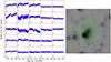 |
Fig. 1. Left: TESS sector 36 light curve of NGC 3783 and nearby pixels. The centre panel labelled ‘source’ is the light curve of the target and the other 24 panels are the light curves of nearby pixels. The red points are the data points with uncertainties greater than the standard deviation of uncertainties from the median of each light curve. Right: TESS image and the locations of NGC 3783 (red circle) and the nearby pixels (green circles) where the light curves on the left were extracted. |
Some sources have anomalous TESS light curves and were discarded. For example, the TESS light curves of 1H 0707−495 (Figure 2) display a periodic behaviour where the flux drops regularly. However, this pattern is observed in most of the nearby pixels, and it is due to contamination from a nearby eclipsing binary. All six TESS sectors are affected by the binary, so we rejected all the TESS light curves of this target for analysis. We confirmed that there are no other similar cases by checking the ASAS-SN variable stars database (Shappee et al. 2014a; Jayasinghe et al. 2018) for variable stars near each target. Similarly, when we observed unusual features in a TESS light curve, we looked at the light curves of nearby pixels to determine if the feature is likely to be real or that the sector should be rejected. Table 1 lists the TESS sectors used for each target and labels which ones are discarded.
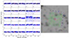 |
Fig. 2. Same as Figure 1 for the TESS sector 6 light curve of 1H 0707−495. The source light curve shows periodic variability due to a nearby eclipsing binary, so this TESS light curve was discarded. |
TESS sectors used for the sample.
The ASAS-SN light curves are measured in millijanskys or magnitudes, while the TESS light curves are measured in units of counts relative to the reference frame. Before we extracted the power spectra, we converted the TESS light curves into millijanskys, using the TESS calibration that one count = 20.44 ± 0.05 mag with a zero point of 2631.9 Jy (Vanderspek et al. 2018).
A representative compilation of light curves (NGC 3783) is shown in Figure 3. It shows that the TESS and ASAS-SN light curves have similar trends with offsets due to the filter differences. The light curves for Circinus are shown in Figure 4. For sectors 11 and 12, a sinusoidal pattern was found in the nearby pixels affecting the target’s light curve, while that pattern is not seen in sector 38. We discarded sectors 11 and 12 and used only sector 38 for the PSD analysis.
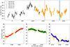 |
Fig. 3. Top: ASAS-SN light curves of NGC 3783 with the TESS sectors marked. Bottom: TESS light curves along with ASAS-SN data. The light curves are scaled to overlap. |
3. Methods
3.1. Power spectra
In general, there are two approaches to constraining PSDs from the light curves: one is the backward method of transforming the light curves into frequency domain and the other is the forward method of assuming a parametric model to fit the light curves. Most previous studies of optical PSDs of AGNs were using the forward method because of the sparse sampling of the light curves (e.g. Kelly et al. 2009; Kozłowski et al. 2010; MacLeod et al. 2010; Zu et al. 2013); however, with the high cadence optical survey, the more intuitive backward method were used in more analyses (e.g. Mushotzky et al. 2011; Burke et al. 2020; Petrecca et al. 2024). Since the forward method can only apply to parametrised PSD models, mostly the DRW model in optical studies, it is beneficial to use the backward methods to infer the general characteristics of the PSD with the inclusion of the new high-frequency TESS data in this paper, which potentially can reveal new PSD features that are absent in commonly assumed optical PSD models. In addition, most previous forward modelling analyses were applied to one dataset, and the computation time and calibration effort will increase significantly when dealing with multiple datasets as in this study. Here, we used a backward Lomb-Scargle periodogram (Lomb 1976; Scargle 1982) to construct the power spectra with simulations to constrain its biases imposed in the PSD break measurement. A forward-fitting analysis will be presented in a separate paper.
The lower frequency limit is set at 1/T, where T = tN − t1 is the time span of the observations, and the upper limit is set at 1/(2ΔTsamp), where ΔTsamp is the typical sampling interval (1 day for ASAS-SN, 30 minutes for TESS sectors ≤26, 10 minutes for TESS sectors > 26). The raw periodograms from the different datasets do not line up perfectly, so we applied several corrections. First, we applied the rms normalisation  (e.g. Vaughan et al. 2003), where
  is the mean flux. Such rms normalisations will also minimise the biases due to the filter differences of the different datasets, assuming that the wavelength-dependent AGN variability mainly manifests in the rms amplitudes (e.g. MacLeod et al. 2010). We next separately normalised the PSDs between the ASAS-SN V- and g-band PSDs, and between the multiple TESS sectors’ PSDs. There can be additional offsets between ASAS-SN and TESS PSD measurements such as differences in the rms variability between wavelengths. It is challenging to normalise the ASAS-SN and TESS PSDs because the ASAS-SN PSDs are dominated by noise in the overlapping region. So we preliminarily normalised the TESS and ASAS-SN components by lining up the PSDs at < 10−2 day−1. Then, for the fitting process, we included the normalisation factor for each PSD as free parameters.
Before fitting, the periodogram is binned and averaged linearly into logarithmic frequency bins with a width of a factor of 1.6 (0.2 dex) in frequency. The uncertainties are the standard deviations about the mean. To estimate any additional systematic error contribution, we fitted a simple power law plus white noise model, P(ν) = Aν−α + C, calculated the reduced χ2 statistic, χred2, and then scaled the uncertainties to make χred2 unity. On average, χred2 before accounting for systematic uncertainties is about 5 for the TESS data, 25 for the V-band ASAS-SN data, and 10 for the g-band ASAS-SN data. Figure 5 shows an example of the periodograms before and after the scaling, binning, and the addition of the estimated systematic uncertainties.
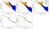 |
Fig. 5. Steps to produce the PSDs used in the model fits. Top: Original Lomb-Scargle periodogram of NGC 3783 (left), with rms normalisation (middle), and after additional scaling to line up the PSDs (right). Bottom: Binned periodogram with the standard deviation of the mean as the uncertainty (left), and with the additional estimated systematic uncertainties (middle). |
3.2. Fitting
We fitted two models to the periodogram, the BPL and DRW models. The main difference between the two models is that the low-frequency and high-frequency power indices are not fixed at 0 and −2, respectively, in the BPL model. We fitted all models by minimising a χ2 statistic. We first fitted a BPL plus white noise model. Compared to the DRW model, this model has several additional parameters, so we approached the fit in several steps. First, we fitted the simple power law with white noise model, P(ν) = Aν−α + C to the individual datasets. Using those fit parameters as initial guesses, the combined periodograms were fit with the smoothly BPL plus white noise power spectrum,
![Mathematical equation: $$ \begin{aligned} P(\nu ) = A_i \left(\frac{\nu }{\nu _{\mathrm{br} }}\right)^{-\alpha _1} \left\{ \frac{1}{2}\left[1+\left(\frac{\nu }{\nu _{\mathrm{br} }}\right)^{1/\Delta }\right]\right\} ^{(\alpha _1-\alpha _2)\Delta }+C_i, \end{aligned} $$](/articles/aa/full_html/2025/06/aa52469-24/aa52469-24-eq6.gif) (1)
(1)
where νbr is the break frequency, Ai is the amplitude at νbr, α1 and α2 are the low and high-frequency slopes, respectively, Δ is the smoothness parameter, where the larger values of Δ mean smoother break, and Ci is the noise level for light curve i (Astropy Collaboration 2022). The parameters νbr, α1, α2, and Δ are the same for all PSDs, while the amplitude Ai and noise Ci are different for each dataset. The adjustments in the amplitudes allow us to account for any remaining normalisation differences between different PSD measurements. We first made fits with Δ fixed at 0.1, 0.2, 0.3, 0.4, and 0.5 and all other parameters free. We found that Δ = 0.1 resulted in the smallest χ2, so we fixed Δ = 0.1 for all subsequent fits. Next, we tested the dependence of χ2 on two model parameters: the TESS-to-ASAS-SN scaling factor and νbr. Though we adjusted the Ai individually, tests showed that the results are very sensitive to the initial conditions. So, we fitted the data on a fixed two-dimensional grid of scaling factor and νbr. The scaling factor that yields the overall lowest χ2 was chosen and the νbr at the χ2 minimum is used as the initial guess for the model, with a ±10% prior constraint on the frequency. Because there are still many parameters to fit, we used the shared value of the amplitude. There are two χ2 minima in some cases, as shown by the example in Figure 6. For these, we separately tried fits at both minima. After this fit, the constant terms Ci were constrained to be within ±10% of the values from the previous fit and the amplitudes Ai were allowed to vary independently. For the final fit, we constrained the amplitudes Ai and noise terms Ci to be within 10% of the prior trial fit values and allowed the power law indices to be free parameters.
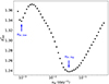 |
Fig. 6. Reduced chi-squared for the BPL model fitting as a function of the break frequencies for MRK 766. The positions we identify as the two break frequencies are labelled. |
We also fitted the DRW model, also known as the continuous-time first-order autoregressive (CAR(1)) process (e.g. Kelly et al. 2009), plus white noise. The DRW model has the power spectrum
 (2)
(2)
where σ is the characteristic timescale and τ is the relaxation time. The relaxation time τ defines the break frequency of νbr = 1/2πτ. Since most previous optical PSD studies did not use light curves with a high cadence of TESS, we fitted the DRW model to both the separate and combined ASAS-SN and TESS PSDs. In general, the DRW fits yield break frequencies in the ASAS-SN frequency regime, which is consistent with previous studies. An example of the combined PSDs with the fits and the corresponding χ2 are shown in Figures 7 and 8.
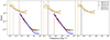 |
Fig. 7. Binned periodogram of NGC 3783 fit with a BPL with the high-frequency break (left), a DRW using both TESS and ASAS-SN data (middle), and using only the ASAS-SN (right), The vertical dashed lines mark the break frequencies. |
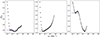 |
Fig. 8. Reduced chi-squared as a function of break frequency for the three fits shown in Figure 7. There are two minima for the DRW fit to the ASAS-SN PSDs, but the minimum at the higher frequency is in the noise-dominated region, so the low-frequency break is used. The dashed blue lines indicate the local minima and the dotted red lines indicate the 1-sigma confidence level. |
3.3. Comparison between long-term ASAS-SN and TESS light curves and PSDs
Since most of the high-frequency breaks lie in the overlapping frequency range of the TESS and ASAS-SN PSDs, it is important to compare TESS and ASAS-SN light curves and PSDs on these timescales for potential calibration issues or variability characteristic differences between filters. Typical TESS Sectors are too short for this purpose. However, TESS observes the ecliptic poles continuously for 13 sectors, so it is possible to extract long-term, nearly continuous TESS light curves for objects near the poles. For this analysis, we used PG 1613+658, a Seyfert I galaxy near the north ecliptic pole observed over Sectors 14 to 26 during the primary mission. The combined light curve is shown in Figure 9.
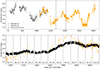 |
Fig. 9. Top: ASAS-SN light curve of PG 1613+658 with the observation window of PG 1613+658 during the TESS primary mission marked. Bottom: TESS primary mission light curve of PG 1613+658 along with the ASAS-SN g-band data. The vertical dashed lines are the sector boundaries. |
We constructed the PSD for the combined TESS light curve using the same procedures to examine if the low-frequency regime of the combined TESS PSDs is consistent with those measured by ASAS-SN, up to a normalisation difference. To do so, we estimated and subtracted the white noise of each PSD. We compared the PSDs of the continuous TESS light curve, the PSDs of ASAS-SN V-band and g-band light curves, and the average of the 13 PSDs for the individual TESS sectors in Figure 10, finding that the TESS and ASAS-SN PSDs are consistent in the overlapping regions and have similar slopes at low frequencies. We did not use the PSD from all 13 sectors because it has strong artificial peaks at 14n (n = 1, 2, 3, …) days created by the observing cadence that strongly affects the fits to the PSD. The results for the BPL PSD fits are shown in Figure 11. Break frequencies measured are  and
and  , which are within the typical range of break frequencies of the AGN sample.
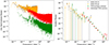 |
Fig. 10. Left: rms-normalised PSDs of PG 1613+658. The PSD in green was constructed using the continuous 13 sector TESS light curve, while the red is the collection of the individual sector PSDs. Right: Binned PSDs with the white noise level subtracted and scaled to line up. The individual TESS sector PSDs were averaged before being binned. |
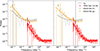 |
Fig. 11. PSDs with the BPL fit of PG 1613+658. The PSDs in red labelled TESS sectors 14-26 are the PSDs of the individual sectors. |
4. Results
From the BPL fits, we find two sets of break frequencies, low- and high-frequency breaks with the dividing line at around 10−2 day−1. The low-frequency breaks νbr, low are measured in objects with only ASAS-SN data, joint fits with TESS and ASAS-SN with a single χred2 minimum below 10−2 day−1, as well as the low-frequency χred2 minimum for joint fits with two χred2 minima. These break frequencies and their associated slopes are similar to those from the DRW fits, meaning that the break frequencies are close to DRW break frequencies and power law indices are about α1 = 0 and α2 = 2. The high-frequency breaks νbr, hig, meaning a χred2 minimum at frequencies higher than 10−2 day−1, are prominent in most targets with both ASAS-SN and TESS data. These νbr, hig are typically in the overlapping region of the ASAS-SN and TESS power spectra. For ASAS-SN, the PSDs at these frequencies are dominated by white noise. For the fits yielding νbr, hig, the power law indices for the low and high frequencies deviate from 0 and 2, especially the low-frequency slopes α1 (Figure 12).
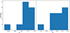 |
Fig. 12. Distribution of the low-frequency (left, α1) and high-frequency (right, α2) slopes for the BPL fits using νbr, hig. |
We have two estimates of the low-frequency break from the DRW models (PSD models for either the ASAS-SN or the ASAS-SN plus TESS data), and a set of low and high-frequency breaks from the BPL fits to the ASAS-SN plus TESS PSDs. All breaks related to the DRW models are in the low-frequency regime. We compare these breaks with the X-ray break frequencies and black hole masses from González-Martín (2018) in Figures 13, 14, and 15. We used the average and uncertainties of X-ray break frequencies presented by González-Martín (2018) Figure 3. To test the relationship between the optical break frequencies and black hole mass and X-ray break frequencies, we computed Pearson’s correlation coefficient (Table 2). We discuss the low and high-frequency regimes separately.
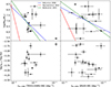 |
Fig. 13. νbr, X and MBH versus νbr = 1/(2πτ) from the DRW model fit on TESS and ASAS-SN PSDs (left), and on ASAS-SN PSDs only (right). |
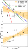 |
Fig. 14. X-ray break frequency νbr, X and MBH versus low optical break frequency νbr, low with the best linear fit and its uncertainties. The upper panel shows similar fits from Kelly et al. (2009), MacLeod et al. (2010), and Burke et al. (2021). |
 |
Fig. 15. Black hole mass and X-ray break frequency versus the high optical break frequencies along with linear fits and their uncertainties. |
Pearson correlation coefficients between break frequencies and previously measured parameters.
4.1. Low-frequency optical breaks
From the three sets of low-frequency optical breaks, we focused on those from the BPL fits, since they correlate better with the black hole mass and X-ray breaks of the sample.
The ranked correlation test shows that the low-frequency break from the BPL fits weakly correlate with both the black hole mass and the X-ray break frequencies with null probabilities of 0.15 and 0.06, respectively. The break versus black hole mass relation is quite consistent with previous relations (Figure 14). We fitted the relationships using
 (3)
(3)
and
 (4)
(4)
We find that  ,
,  ,
,  , and
, and  , with the results shown in Figure 14. Although the relation between νbr, low and MBH is not statistically significant in this paper, we list our relation as a comparison with previous studies, who found the relation significant (e.g. Kelly et al. 2009; MacLeod et al. 2010; Burke et al. 2021). PG 1613+658, the Seyfert I galaxy with 13 continuous TESS sectors discussed earlier, has a reverberation mapping black hole mass measurement of
  (Kaspi et al. 2000). Using the break frequency from the PSD of the continuous TESS light curve and this MBH − νbr relationship (Equation 4), we get
  , which agrees with the previous measurement.
4.2. High-frequency optical breaks
The high-frequency optical breaks were detected in the BPL fits to the combined ASAS-SN and TESS PSDs. They are all at frequencies above 10−2 day−1, and resemble the steepening of optical PSDs found in Kepler data (Mushotzky et al. 2011; Kasliwal et al. 2015; Aranzana et al. 2018; Smith et al. 2018). Here, we can compare them with the X-ray break frequencies measured for the same set of objects. The high-frequency optical νbr, hig and X-ray νbr, X break frequencies are given in Table 3 along with MBH and shown in Figure 15. The ranked correlation test shows that the high-frequency optical breaks and X-ray breaks are correlated with a null probability of 4%. We also find a hint of a correlation between the high-frequency breaks and the black hole masses, but at lower significance with a null probability of 6%. Figure 15 shows fits to the correlations using
 (5)
(5)
Properties of the AGN sample.
and
 (6)
(6)
With these equations we find that  ,
,  ,
,  , and
, and  . If we apply this MBH − νbr relationship to PG 1613+658, we get
  , which does not agree with the previous measurement. Further studies are needed to evaluate the validity of this relationship.
We find that the slopes of the BPL fits do not have a strong correlation with the black hole mass or the break frequency. The Pearson’s correlation test parameters are r = −0.17 and p = 0.63 for α1 − MBH, r = 0.33 and p = 0.32 for α1 − νbr, hig, r = −0.38 and p = 0.28 for α2 − MBH, and r = −0.22 and p = 0.51 for α2 − νbr, hig pairs.
4.3. Testing the PSD fitting method
To determine whether our PSD fitting method is robust and ensure that the high-frequency breaks are not simply artefacts of combining two sets of PSDs, we selected a number of model parameters, simulated light curves, and performed the PSD fits method as described in Section 3 to test if the true model parameters can be recovered. We used the method of Timmer & Koenig (1995) to simulate light curves of a given PSD. Then we added white noise and applied the same sampling windows as the observations. To account for potential misestimation of the measurement noise, we used the three-point method to scale the original measurement uncertainty; we checked three consecutive data points within a certain time frame, find the linear fit, and find the scaling factor for the measurement uncertainties such that χ2 = 1. This process was repeated for each ASAS-SN and TESS light curve. For this testing, we started with a specific set of parameters, and changed one parameter at a time. We used two different sets of initial parameter sets:  , α1 = 0.3, and α2 = 2.1, which correspond to the typical values for low-frequency breaks, and
  , α1 = 1.2, and α2 = 2.1, which correspond to the typical values for high-frequency breaks. The ranges of parameters are 0.0 ≤ α1 ≤ 1.5, 1.5 ≤ α2 ≤ 3.0 with steps of 0.3, and −2.8 ≤ log νbr ≤ −1.0 with steps of a 0.3 dex.
The results are shown on Figure 16. We observe varying levels of biases between the best-fit and input model parameter values. However, the biases can be estimated. For the break frequency, we find that the input and measured break frequencies have an approximately linear relationship, but with offsets. With a shallow α1 (varying from the low-frequency break setup), measured break frequencies deviate more towards larger values at lower frequencies. With a steeper α1 (varying form the high-frequency break setup), cases with more TESS sectors show better agreement, while having fewer TESS sectors appears to lead to almost constant values. For both cases, the discrepancy is greatest at the lowest break frequency, but that may be caused by the fact that it is near the PSD lower frequency measurement limit. For power law indices, it appears the measured values have some upper limit to what this method can measure.
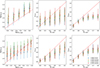 |
Fig. 16. Comparisons of BPL model parameters from the PSD fitting method and the true values used for light curve simulations. Variations from the low-frequency and high-frequency break parameters are shown on top and bottom panels, respectively. The dashed red line in each panel represents the one-to-one relation. The data points are slightly offset along the x-axis to make them distinguishable. |
To determine which factor contributes the most to the observed discrepancies, we tried using simulated light curves by adding different observational biases one at a time. We tested adding white noise, our treatment of measurement uncertainties, and the effect of observing sampling windows. We used the three simulated TESS sectors for the tests. We find that the light curve sampling window affects the results the most (Figure 17), while the white noise and our treatment of measurement uncertainties had little effect on the measured PSD parameters. Since the sampling window effect is significant for ASAS-SN, it makes sense that the discrepancy is greater when there are fewer TESS sectors, where the ASAS-SN PSDs contribute more to the fit. In summary, Figures 16 and 17 show that combining two sets of PSDs from TESS and ASAS-SN introduces a bias on measured break frequency towards higher values. However, the measured values are mostly consistent with true values, suggesting that the νbr, hig we measured are not due to combining PSDs.
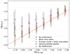 |
Fig. 17. Measured break frequencies with different levels of modifications on the light curves versus the input break frequencies for the light curve simulations. The dashed red line represents the one-to-one relation. The data points are slightly offset along the x-axis to make them distinguishable. |
We also attempted calculating the correction for the measured high-frequency break. After correction, the linear trend is still there, but the error bars are much larger and the slope is much shallower (Figure 18). The newly measured correlation parameters are  ,
,  ,
,  , and
, and  , with the correlation null probabilities of 0.02 and 0.02. With the break frequency correction,
  of PG 1613+658 becomes −0.68 ± 1.72, and with the new correlation parameters, its black hole mass is
  . Compared to the reverberation mapping measurement, the difference in central values is still large, the two values agree within 2σ because of the large uncertainties in the correlation.
4.4. Multi-variable correlation plane
A number of studies have explored the correlation between the X-ray break frequency and black hole mass, and also examines how other parameters, such as bolometric luminosity and obscuration, can better constrain that correlation (e.g. McHardy et al. 2006; González-Martín & Vaughan 2012; González-Martín 2018). We also tested if our newly found correlations are affected by the obscuration, bolometric luminosity, X-ray luminosity, optical luminosity, or optical-to-X-ray luminosity ratio. González-Martín (2018) reports the range of values of NH and Lbol for the sample. The reported Lbol is derived from the X-ray luminosity at 2−10 keV:
 (7)
(7)
where ℒ = log(Lbol/L⊙)−12 (Marconi et al. 2004). We used the middle values from the range of NH and Lbol reported by González-Martín (2018) and derived LX from Lbol. For optical luminosity, we used the median ASAS-SN V-band magnitude, after correcting for galactic reddening and K-correction, to estimate the V-band luminosity of the sample.
We fitted the multi-variable correlation,
 (8)
(8)
where Y is either log νbr, X or log MBH and log νbr, opt is the optical break frequency (log νbr, low, log νbr, hig, or log νbr, hig, corr), X is log NH, log Lbol, log LX, log LV, or log(LV/LX) and β, γ, and δ are constants for fitting. We tested all combinations with X, Y, and log νbr, opt. In most cases, the best-fit β values are consistent with the 1σ range of the original two-parameter correlation values. For some of the combinations, |β| approaches zero for the best fit, and the multi-variable correlation is driven by the parameters Y and X. These cases are not related to the main goal of this paper, which is to explore the correlations related to νbr, opt of either high or low frequencies. Thus, we fixed β values at the best-fit values from the two-parameter correlations for these cases.
We find that, for all combinations, the correlations improve significantly with the addition of X-ray or optical luminosity and slightly with the addition of optical-to-X-ray luminosity ratio or obscuration. The only exception is νbr, low − log MBH correlation with the addition of log NH, which had nearly no improvement. For all the multi-variate correlations with the additional X-ray or optical luminosity parameter we tested, the median significance has improved to p = 0.01 compared to the median significance of p = 0.05 when considering only the original two parameter correlations. By nature of bolometric luminosity being derived from the X-ray luminosity, the effect of adding Lbol is nearly the same as adding LX. For example, the original two-parameter correlation between log νbr, hig and log νX has the correlation coefficient of r = 0.57 with p = 0.04. With the addition of log Lbol, log LX, or log LV, the correlation coefficient becomes r = 0.73 with p = 0.005, r = 0.73 with p = 0.005, and r = 0.69 with p = 0.009, respectively (Figure 19). We present the entirety of our multi-variable fit results in Appendix B.
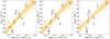 |
Fig. 19. Results of fitting the correlation between log νbr, X and log νbr, hig with the addition of Lbol (left), log LX (middle), or log LV (right). The dark and lightly shaded regions represent the 68% and 95% confidence ranges, respectively. |
5. Summary and discussion
We studied AGN variability over six orders of magnitude from minute to decade timescales by combining TESS and ASAS-SN light curves. Our analysis shows that the ASAS-SN and TESS PSDs can be jointly modelled with a normalisation offset due to differences in noise levels and filters. We analysed PG 1613+658, a brigh target in the TESS continuous monitoring regions, that had a TESS light curve spanning more than a year, meaning that there is a significant overlap between PSDs, and found consistent light curves and PSD measurements.
We also compared our results to scaling relations between the low-frequency break and black hole mass from Kelly et al. (2009), MacLeod et al. (2010), and Burke et al. (2021). To compare with the multi-variate correlation from MacLeod et al. (2010), we used their relations assuming a rest frame wavelength of λRF = 8000 Å, an absolute magnitude of Mi = −21.3, and a redshift of z = 0.02. All three relations are shown in Figures 13 and 14.
The νbr − MBH relationship found using the various DRW fits does not agree with previous studies very well, though the DRW PSD fits that use TESS and ASAS-SN have a similar trend (Figure 13). Although the correlations between these DRW break frequencies and X-ray break frequencies are not significant, as can be seen in the bottom panels in Figure 13, the X-ray break dependence on the DRW breaks is almost flat, which is contrary to the slope of  between the low-frequency breaks from the BPL model and X-ray breaks.
Burke et al. (2020) performed a similar break frequency analysis on NGC 4395. They used the TESS sector 22 light curve to construct the PSD and fit a BPL. They find a break frequency of  , which differs from our value of
  . This may be due to our using both TESS and ASAS-SN data. Using only the TESS PSDs, we find
  , which agrees with Burke et al. (2020).
Active galactic nucleus variability PSDs are generally characterised by power laws with breaks; distinct break frequencies have been observed in both optical (e.g. Kelly et al. 2009; MacLeod et al. 2010; Simm et al. 2016; Burke et al. 2021) and X-ray data (e.g. Uttley et al. 2002; Markowitz et al. 2003; González-Martín & Vaughan 2012; González-Martín 2018). Both the optical and X-ray break frequencies are correlated with the black hole mass, but with different scaling relations (e.g. Simm et al. 2016; Burke et al. 2021). The fact that the break frequency and black hole mass have a statistically significant correlation suggests that the AGN variability is closely related to accretion physics.
This paper presents the first analysis comparing optical and X-ray PSDs by exploiting the all-sky nature of the ASAS-SN and TESS surveys. We find a set of high-frequency breaks (≳10−2 day−1) in the joint optical light curves. These high-frequency breaks were previously observed as a steepening of the optical PSD at high frequencies (Mushotzky et al. 2011; Kasliwal et al. 2015; Aranzana et al. 2018; Smith et al. 2018). We find a potential correlation between the X-ray and high-frequency optical break frequencies. The slope of the power law relation of  is close to a relation of β3 = 0.5, given the uncertainty, which is shallower than a simple proportional relation of β3 = 1. We can interpret the offset between the optical and X-ray break frequencies as the light crossing time between the X-ray and optical emission regions. A slope shallower than a proportional relation implies that the X-ray emission region is smaller than the optical for higher MBH. There is also an indication that the high-frequency optical breaks may be correlated with the black hole mass, albeit weakly. This could be a new scaling relationship νbr − MBH, different from those found in previous studies, providing an alternative method for estimating the black hole mass. However, with corrections for sampling, the correlations between the high-frequency breaks and X-ray break frequencies and the black hole mass become less significant. A larger sample is needed to better establish the correlation with more accurate slope measurements.
We further explored whether the correlations discussed in this paper are affected by the X-ray luminosity, optical luminosity, optical-to-X-ray luminosity ratio, or obscuration. We find that including the X-ray, optical, or bolometric luminosity as the third parameter can significantly improve the correlation significances, the optical-to-X-ray luminosity ratio or obscuration only modestly improves the correlation significances. With the inclusion of an additional parameter, the dependence between the X-ray and high-frequency optical break has a power law slope of β3 in the range 0.1 to 0.8 with a median value of 0.52 (Table B.1), which is consistent with the original two-parameter slope of β3 = 0.59 ± 0.27.
If the optical and X-ray frequencies are indeed correlated, we can speculate on the implications. The X-ray emission is produced from inverse Compton scattering between UV seed photons from the accretion disc and electrons in the corona. The X-ray emission then irradiates the accretion disc, heating the disc and modifying the optical emission. Therefore, the optical and X-ray variability should show correlations. In fact, short-timescale correlations between optical and X-ray light curves are well established and used as a tool in continuous reverberation mapping studies to constrain optical and X-ray emission sizes (e.g. Shappee et al. 2014b; Edelson et al. 2015; Troyer et al. 2016; McHardy et al. 2018). The correlation we find between the X-ray and optical PSD break frequencies provides independent support that the optical and X-ray emissions are closely related on short timescales. Since the optical PSD on these scales deviates from the extrapolation from longer timescales, the variation in the X-ray emission, through ‘reprocessing’, can be the main driver for the interaction between optical and X-ray emission on short timescales.
The X-ray emission, which can vary on very short timescales, is speculated to come from the innermost part of the AGN, near the SMBH. On the other hand, the optical emission is believed to come from the accretion disc. Studies in quasar microlensing (e.g. Morgan et al. 2008; Dai et al. 2010) and reverberation mapping (e.g. Shappee et al. 2014b; Edelson et al. 2015; Cackett et al. 2018; Jha et al. 2022) find that the sizes of X-ray and optical emission regions range from 1014 to 1015 cm and from 1015 to 1016 cm, respectively. This scale is comparable to our observed difference in characteristic timescales, with τ = 1/(2πνbr)∼10−2 day for the X-rays and ∼100 days for the optical.
In the low-frequency regime (≲10−2 day−1), we also find a correlation between the optical and X-ray breaks, with a similar slope  . Our analysis results show that the DRW model fits the ASAS-SN PSDs well. We also roughly recover the DRW break versus black hole mass relation measured in the literature. When high-frequency TESS PSDs are introduced, the DRW work less well. The BPL fits show that the power law indices deviate from the DRW values of 0 and −2, as shown on the distributions on Figure 12, especially for the low-frequency slope. A few objects potentially have two break frequencies, according to the BPL fits (Figure 6). This means that AGN variability is more complicated and may be governed by different physical processes at different scales. For example, the longer-term variability could be mainly described by a DRW model, physically related to magnetorotational instability or other disc variability mechanisms (e.g. Kelly et al. 2009; MacLeod et al. 2010), while the short-term optical variability is strongly affected by other variability mechanisms, such as the reprocessing of X-rays.
Data availability
The full Tables A.1 and A.2 are available at the CDS via anonymous ftp to cdsarc.cds.unistra.fr (130.79.128.5) or via https://cdsarc.cds.unistra.fr/viz-bin/cat/J/A+A/698/A105
Acknowledgments
We thank the anonymous referee for constructive suggestions. H.Y. and X.D. would like to acknowledge NASA funds 80NSSC22K0488, 80NSSC23K0379 and NSF fund AAG2307802. H.Y. thank the Avenir fellowship. We also thank the OU Supercomputing Center for Education & Research (OSCER) at the University of Oklahoma for providing the computing resources.
References
- Alard, C. 2000, A&AS, 144, 363 [NASA ADS] [CrossRef] [EDP Sciences] [Google Scholar]
- Alard, C., & Lupton, R. H. 1998, ApJ, 503, 325 [Google Scholar]
- Aranzana, E., Körding, E., Uttley, P., Scaringi, S., & Bloemen, S. 2018, MNRAS, 476, 2501 [Google Scholar]
- Astropy Collaboration (Price-Whelan, A. M., et al.) 2022, ApJ, 935, 167 [NASA ADS] [CrossRef] [Google Scholar]
- Balbus, S. A., & Hawley, J. F. 1991, ApJ, 376, 214 [Google Scholar]
- Burke, C. J., Shen, Y., Chen, Y.-C., et al. 2020, ApJ, 899, 136 [Google Scholar]
- Burke, C. J., Shen, Y., Blaes, O., et al. 2021, Science, 373, 789 [NASA ADS] [CrossRef] [Google Scholar]
- Butler, N. R., & Bloom, J. S. 2011, AJ, 141, 93 [Google Scholar]
- Cackett, E. M., Chiang, C.-Y., McHardy, I., et al. 2018, ApJ, 857, 53 [NASA ADS] [CrossRef] [Google Scholar]
- Dai, X., Kochanek, C. S., Chartas, G., et al. 2010, ApJ, 709, 278 [Google Scholar]
- Dexter, J., & Agol, E. 2011, ApJ, 727, L24 [Google Scholar]
- Edelson, R., Gelbord, J. M., Horne, K., et al. 2015, ApJ, 806, 129 [NASA ADS] [CrossRef] [Google Scholar]
- Fausnaugh, M. M., Vallely, P. J., Kochanek, C. S., et al. 2021, ApJ, 908, 51 [NASA ADS] [CrossRef] [Google Scholar]
- González-Martín, O. 2018, ApJ, 858, 2 [Google Scholar]
- González-Martín, O., & Vaughan, S. 2012, A&A, 544, A80 [NASA ADS] [CrossRef] [EDP Sciences] [Google Scholar]
- Grandi, P., Tagliaferri, G., Giommi, P., Barr, P., & Palumbo, G. G. C. 1992, ApJS, 82, 93 [Google Scholar]
- Haardt, F., & Maraschi, L. 1991, ApJ, 380, L51 [Google Scholar]
- Henden, A. A., Levine, S., Terrell, D., & Welch, D. L. 2015, Am. Astron. Soc. Meet. Abstr., 225, 336.16 [Google Scholar]
- Jayasinghe, T., Kochanek, C. S., Stanek, K. Z., et al. 2018, MNRAS, 477, 3145 [Google Scholar]
- Jayasinghe, T., Stanek, K. Z., Kochanek, C. S., et al. 2019, MNRAS, 485, 961 [Google Scholar]
- Jha, V. K., Joshi, R., Chand, H., et al. 2022, MNRAS, 511, 3005 [NASA ADS] [CrossRef] [Google Scholar]
- Kasliwal, V. P., Vogeley, M. S., & Richards, G. T. 2015, MNRAS, 451, 4328 [CrossRef] [Google Scholar]
- Kaspi, S., Smith, P. S., Netzer, H., et al. 2000, ApJ, 533, 631 [Google Scholar]
- Kawaguchi, T., Mineshige, S., Umemura, M., & Turner, E. L. 1998, ApJ, 504, 671 [NASA ADS] [CrossRef] [Google Scholar]
- Kelly, B. C., Bechtold, J., & Siemiginowska, A. 2009, ApJ, 698, 895 [Google Scholar]
- Kochanek, C. S., Shappee, B. J., Stanek, K. Z., et al. 2017, PASP, 129, 104502 [Google Scholar]
- Kozłowski, S. 2016, ApJ, 826, 118 [CrossRef] [Google Scholar]
- Kozłowski, S., Kochanek, C. S., Udalski, A., et al. 2010, ApJ, 708, 927 [CrossRef] [Google Scholar]
- Lightman, A. P., & Eardley, D. M. 1974, ApJ, 187, L1 [Google Scholar]
- Lomb, N. R. 1976, Ap&SS, 39, 447 [Google Scholar]
- MacLeod, C. L., Ivezić, Ž., Kochanek, C. S., et al. 2010, ApJ, 721, 1014 [Google Scholar]
- MacLeod, C. L., Brooks, K., Ivezić, Ž., et al. 2011, ApJ, 728, 26 [NASA ADS] [CrossRef] [Google Scholar]
- Marconi, A., Risaliti, G., Gilli, R., et al. 2004, MNRAS, 351, 169 [Google Scholar]
- Markowitz, A., Edelson, R., & Vaughan, S. 2003, ApJ, 598, 935 [NASA ADS] [CrossRef] [Google Scholar]
- McHardy, I. M., Papadakis, I. E., Uttley, P., Page, M. J., & Mason, K. O. 2004, MNRAS, 348, 783 [NASA ADS] [CrossRef] [Google Scholar]
- McHardy, I. M., Koerding, E., Knigge, C., Uttley, P., & Fender, R. P. 2006, Nature, 444, 730 [NASA ADS] [CrossRef] [Google Scholar]
- McHardy, I. M., Connolly, S. D., Horne, K., et al. 2018, MNRAS, 480, 2881 [NASA ADS] [CrossRef] [Google Scholar]
- Morgan, C. W., Kochanek, C. S., Dai, X., Morgan, N. D., & Falco, E. E. 2008, ApJ, 689, 755 [Google Scholar]
- Mushotzky, R. F., Done, C., & Pounds, K. A. 1993, ARA&A, 31, 717 [NASA ADS] [CrossRef] [Google Scholar]
- Mushotzky, R. F., Edelson, R., Baumgartner, W., & Gandhi, P. 2011, ApJ, 743, L12 [NASA ADS] [CrossRef] [Google Scholar]
- Peterson, B. M., Bentz, M. C., Desroches, L.-B., et al. 2005, ApJ, 632, 799 [NASA ADS] [CrossRef] [Google Scholar]
- Petrecca, V., Papadakis, I. E., Paolillo, M., De Cicco, D., & Bauer, F. E. 2024, A&A, 686, A286 [NASA ADS] [CrossRef] [EDP Sciences] [Google Scholar]
- Ptak, A., Yaqoob, T., Mushotzky, R., Serlemitsos, P., & Griffiths, R. 1998, ApJ, 501, L37 [NASA ADS] [CrossRef] [Google Scholar]
- Reynolds, C. S., & Miller, M. C. 2009, ApJ, 692, 869 [Google Scholar]
- Ricker, G. R., Winn, J. N., Vanderspek, R., et al. 2015, JATIS, 1, 014003 [Google Scholar]
- Ruan, J. J., Anderson, S. F., MacLeod, C. L., et al. 2012, ApJ, 760, 51 [Google Scholar]
- Scargle, J. D. 1982, ApJ, 263, 835 [Google Scholar]
- Shakura, N. I., & Sunyaev, R. A. 1976, MNRAS, 175, 613 [NASA ADS] [CrossRef] [Google Scholar]
- Shappee, B., Prieto, J., Stanek, K. Z., et al. 2014a, Am. Astron. Soc. Meet. Abstr., 223, 236.03 [Google Scholar]
- Shappee, B. J., Prieto, J. L., Grupe, D., et al. 2014b, ApJ, 788, 48 [Google Scholar]
- Simm, T., Salvato, M., Saglia, R., et al. 2016, A&A, 585, A129 [NASA ADS] [CrossRef] [EDP Sciences] [Google Scholar]
- Smith, K. L., Mushotzky, R. F., Boyd, P. T., et al. 2018, ApJ, 857, 141 [NASA ADS] [CrossRef] [Google Scholar]
- Timmer, J., & Koenig, M. 1995, A&A, 300, 707 [NASA ADS] [Google Scholar]
- Treiber, H. P., Hinkle, J. T., Fausnaugh, M. M., et al. 2022, ArXiv e-prints [arXiv:2209.15019] [Google Scholar]
- Trèvese, D., & Vagnetti, F. 2002, ApJ, 564, 624 [Google Scholar]
- Troyer, J., Starkey, D., Cackett, E. M., et al. 2016, MNRAS, 456, 4040 [Google Scholar]
- Uttley, P., McHardy, I. M., & Papadakis, I. E. 2002, MNRAS, 332, 231 [Google Scholar]
- Vallely, P. J., Kochanek, C. S., Stanek, K. Z., Fausnaugh, M., & Shappee, B. J. 2021, MNRAS, 500, 5639 [Google Scholar]
- Vanden Berk, D. E., Wilhite, B. C., Kron, R. G., et al. 2004, ApJ, 601, 692 [Google Scholar]
- Vanderspek, R., Doty, J. P., Fausnaugh, M., et al. 2018, TESS Instrument Handbook, Tech. Rep., Kavli Institute for Astrophysics and Space Science, Massachusetts Institute of Technology [Google Scholar]
- Vaughan, S., Edelson, R., Warwick, R. S., & Uttley, P. 2003, MNRAS, 345, 1271 [Google Scholar]
- Wandel, A., Peterson, B. M., & Malkan, M. A. 1999, ApJ, 526, 579 [NASA ADS] [CrossRef] [Google Scholar]
- Yuk, H., Dai, X., Jayasinghe, T., et al. 2022, ApJ, 930, 110 [NASA ADS] [CrossRef] [Google Scholar]
- Zu, Y., Kochanek, C. S., Kozłowski, S., & Udalski, A. 2013, ApJ, 765, 106 [NASA ADS] [CrossRef] [Google Scholar]
Appendix A: Light curve compilation
Here, we present the compilation of light curves used for this study in both text and visual formats. ASAS-SN and TESS light curves are shown in Tables A.1 and A.2 and Figures A.1, A.2, and A.3.
ASAS-SN light curves used for this study (extract).
TESS light curves used for this study (extract).
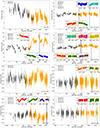 |
Fig. A.1. ASAS-SN light curves of MRK 335, ESO 113-G010, Fairall 9, PKS 0558-504, 1H 0707-495, ESO 434-G040, NGC 3227, and RE J1034+396. The TESS sectors are marked and shown in the insets. The light curves are scaled to overlap. |
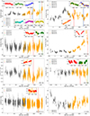 |
Fig. A.2. Continuation of Figure A.1, for NGC 3516, NGC 3783, NGC 4051, NGC 4151, MRK 766, NGC 4395, MCG-06-30-15, and IC 4329A. |
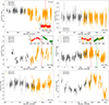 |
Fig. A.3. Continuation of Figure A.1, for Circinus, NGC 5506, NGC 5548, NGC 6860, ARK 564, and NGC 7469. |
Appendix B: Multi-variable correlation fitting results
In this section, we present the results of fitting the multi-variable correlations (Equation 8). Figures B.1 and B.2 show the fitting plots with the addition of X-ray and V-band luminosities, which improved the fit the most. Table B.1 lists all values we obtained from the fits. The units used for νbr, MBH, NH, and L are day−1, M⊙, cm−2, and erg s−1, respectively.
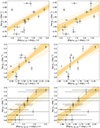 |
Fig. B.1. Multi-variable correlation between X-ray break frequency and different optical break frequencies–log νbr, low (top), log νbr, hig (middle), and log νbr, hig, corr (bottom)–with the addition of X-ray luminosity (left) or V-band luminosity (right). The dark and lightly shaded regions represent the 68% and 95% confidence ranges, respectively. |
Parameters obtained from multi-variable correlation fittings to Equation 8 and Pearson correlation strength and null probability.
All Tables
Pearson correlation coefficients between break frequencies and previously measured parameters.
Parameters obtained from multi-variable correlation fittings to Equation 8 and Pearson correlation strength and null probability.
All Figures
|
Fig. 1. Left: TESS sector 36 light curve of NGC 3783 and nearby pixels. The centre panel labelled ‘source’ is the light curve of the target and the other 24 panels are the light curves of nearby pixels. The red points are the data points with uncertainties greater than the standard deviation of uncertainties from the median of each light curve. Right: TESS image and the locations of NGC 3783 (red circle) and the nearby pixels (green circles) where the light curves on the left were extracted. |
| In the text | |
|
Fig. 2. Same as Figure 1 for the TESS sector 6 light curve of 1H 0707−495. The source light curve shows periodic variability due to a nearby eclipsing binary, so this TESS light curve was discarded. |
| In the text | |
|
Fig. 3. Top: ASAS-SN light curves of NGC 3783 with the TESS sectors marked. Bottom: TESS light curves along with ASAS-SN data. The light curves are scaled to overlap. |
| In the text | |
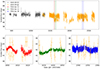 |
Fig. 4. Same as Figure 3 for Circinus with TESS sectors 11, 12, and 38. |
| In the text | |
|
Fig. 5. Steps to produce the PSDs used in the model fits. Top: Original Lomb-Scargle periodogram of NGC 3783 (left), with rms normalisation (middle), and after additional scaling to line up the PSDs (right). Bottom: Binned periodogram with the standard deviation of the mean as the uncertainty (left), and with the additional estimated systematic uncertainties (middle). |
| In the text | |
|
Fig. 6. Reduced chi-squared for the BPL model fitting as a function of the break frequencies for MRK 766. The positions we identify as the two break frequencies are labelled. |
| In the text | |
|
Fig. 7. Binned periodogram of NGC 3783 fit with a BPL with the high-frequency break (left), a DRW using both TESS and ASAS-SN data (middle), and using only the ASAS-SN (right), The vertical dashed lines mark the break frequencies. |
| In the text | |
|
Fig. 8. Reduced chi-squared as a function of break frequency for the three fits shown in Figure 7. There are two minima for the DRW fit to the ASAS-SN PSDs, but the minimum at the higher frequency is in the noise-dominated region, so the low-frequency break is used. The dashed blue lines indicate the local minima and the dotted red lines indicate the 1-sigma confidence level. |
| In the text | |
|
Fig. 9. Top: ASAS-SN light curve of PG 1613+658 with the observation window of PG 1613+658 during the TESS primary mission marked. Bottom: TESS primary mission light curve of PG 1613+658 along with the ASAS-SN g-band data. The vertical dashed lines are the sector boundaries. |
| In the text | |
|
Fig. 10. Left: rms-normalised PSDs of PG 1613+658. The PSD in green was constructed using the continuous 13 sector TESS light curve, while the red is the collection of the individual sector PSDs. Right: Binned PSDs with the white noise level subtracted and scaled to line up. The individual TESS sector PSDs were averaged before being binned. |
| In the text | |
|
Fig. 11. PSDs with the BPL fit of PG 1613+658. The PSDs in red labelled TESS sectors 14-26 are the PSDs of the individual sectors. |
| In the text | |
|
Fig. 12. Distribution of the low-frequency (left, α1) and high-frequency (right, α2) slopes for the BPL fits using νbr, hig. |
| In the text | |
|
Fig. 13. νbr, X and MBH versus νbr = 1/(2πτ) from the DRW model fit on TESS and ASAS-SN PSDs (left), and on ASAS-SN PSDs only (right). |
| In the text | |
|
Fig. 14. X-ray break frequency νbr, X and MBH versus low optical break frequency νbr, low with the best linear fit and its uncertainties. The upper panel shows similar fits from Kelly et al. (2009), MacLeod et al. (2010), and Burke et al. (2021). |
| In the text | |
|
Fig. 15. Black hole mass and X-ray break frequency versus the high optical break frequencies along with linear fits and their uncertainties. |
| In the text | |
|
Fig. 16. Comparisons of BPL model parameters from the PSD fitting method and the true values used for light curve simulations. Variations from the low-frequency and high-frequency break parameters are shown on top and bottom panels, respectively. The dashed red line in each panel represents the one-to-one relation. The data points are slightly offset along the x-axis to make them distinguishable. |
| In the text | |
|
Fig. 17. Measured break frequencies with different levels of modifications on the light curves versus the input break frequencies for the light curve simulations. The dashed red line represents the one-to-one relation. The data points are slightly offset along the x-axis to make them distinguishable. |
| In the text | |
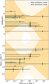 |
Fig. 18. Same as Figure 15, but with νbr, hig corrected for distortion. |
| In the text | |
|
Fig. 19. Results of fitting the correlation between log νbr, X and log νbr, hig with the addition of Lbol (left), log LX (middle), or log LV (right). The dark and lightly shaded regions represent the 68% and 95% confidence ranges, respectively. |
| In the text | |
|
Fig. A.1. ASAS-SN light curves of MRK 335, ESO 113-G010, Fairall 9, PKS 0558-504, 1H 0707-495, ESO 434-G040, NGC 3227, and RE J1034+396. The TESS sectors are marked and shown in the insets. The light curves are scaled to overlap. |
| In the text | |
|
Fig. A.2. Continuation of Figure A.1, for NGC 3516, NGC 3783, NGC 4051, NGC 4151, MRK 766, NGC 4395, MCG-06-30-15, and IC 4329A. |
| In the text | |
|
Fig. A.3. Continuation of Figure A.1, for Circinus, NGC 5506, NGC 5548, NGC 6860, ARK 564, and NGC 7469. |
| In the text | |
|
Fig. B.1. Multi-variable correlation between X-ray break frequency and different optical break frequencies–log νbr, low (top), log νbr, hig (middle), and log νbr, hig, corr (bottom)–with the addition of X-ray luminosity (left) or V-band luminosity (right). The dark and lightly shaded regions represent the 68% and 95% confidence ranges, respectively. |
| In the text | |
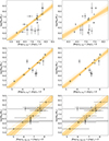 |
Fig. B.2. Same as Figure B.1, but with MBH instead of νbr, X. |
| In the text | |
Current usage metrics show cumulative count of Article Views (full-text article views including HTML views, PDF and ePub downloads, according to the available data) and Abstracts Views on Vision4Press platform.
Data correspond to usage on the plateform after 2015. The current usage metrics is available 48-96 hours after online publication and is updated daily on week days.
Initial download of the metrics may take a while.