| Issue |
A&A
Volume 685, May 2024
|
|
|---|---|---|
| Article Number | A163 | |
| Number of page(s) | 21 | |
| Section | Extragalactic astronomy | |
| DOI | https://doi.org/10.1051/0004-6361/202347966 | |
| Published online | 20 May 2024 | |
High-z gamma-ray burst detection by SVOM/ECLAIRs: Impact of instrumental biases on the bursts’ measured properties
IRAP, Université de Toulouse, CNRS, CNES, UPS, Toulouse, France
e-mail: Miguel.Llamas.Lanza@gmail.com
Received:
14
September
2023
Accepted:
23
February
2024
Context. Gamma-ray bursts (GRBs) can be detected at cosmological distances, and therefore can be used to study the contents and phases of the early Universe. The 4−150 keV wide-field trigger camera ECLAIRs on board the Space-based multi-band Variable Object Monitor (SVOM) mission, dedicated to studying the high-energy transient sky in synergy with multi-messenger follow-up instruments, has been adapted to detect high-z GRBs.
Aims. Investigating the detection capabilities of ECLAIRs for high-redshift GRBs and estimating the impacts of instrumental biases in reconstructing some of the source measured properties, focusing on GRB duration biases as a function of redshift.
Methods. We simulated realistic detection scenarios for a sample of 162 already observed GRBs with known redshift values as they would have been seen by ECLAIRs. We simulated them at redshift values equal to and higher than their measured value. Then we assessed whether they would be detected with a trigger algorithm resembling that on board ECLAIRs, and derived quantities, such as T90, for those that would have been detected.
Results. We find that ECLAIRs would be capable of detecting GRBs up to very high redshift values (e.g. 20 GRBs in our sample are detectable within more than 0.4 of the ECLAIRs field of view for zsim > 12). The ECLAIRs low-energy threshold of 4 keV, contributes to this great detection capability, as it may enhance it at high redshift (z > 10) by over 10% compared with a 15 keV low-energy threshold. We also show that the detection of GRBs at high-z values may imprint tip-of-the-iceberg biases on the GRB duration measurements, which can affect the reconstruction of other source properties.
Key words: gamma-ray burst: general / galaxies: high-redshift
© The Authors 2024
 Open Access article, published by EDP Sciences, under the terms of the Creative Commons Attribution License (https://creativecommons.org/licenses/by/4.0), which permits unrestricted use, distribution, and reproduction in any medium, provided the original work is properly cited.
This article is published in open access under the Subscribe to Open model. Subscribe to A&A to support open access publication.
1. Introduction
Gamma-ray bursts (GRBs) are powerful transient events emitting large amounts of energy in X-rays and γ-rays (Klebesadel et al. 1973; Zhang 2007, 2018; Vedrenne & Atteia 2009). They are characterised by a short, highly variable and intense phase called prompt emission, followed by a multi-wavelength long-lasting afterglow emission characterised by a rapid flux decay (Costa et al. 1997; Van Paradijs et al. 1997; Zhang et al. 2006; Nousek et al. 2006; Laskar et al. 2023). They are thought to signal the catastrophic formation of a compact object, for example a black hole (BH) or a neutron star (NS), and the launch of powerful ultra-relativistic jets (e.g. Piran 2005; Kumar & Zhang 2015) following either the merger of a binary NS or a binary BH-NS (Eichler et al. 1989; Tanvir et al. 2013; Abbott et al. 2017) or the core collapse of some massive stars, with masses M ≳ 30 M⊙ (Woosley 1993; Galama et al. 1999; Hjorth et al. 2003; Woosley & Bloom 2006; Melandri et al. 2019). These two different physical events are typically associated with short and long GRBs, respectively. Nevertheless, the overlap in the duration of these two populations defies their classification based solely on this parameter (Bromberg et al. 2013). A new class has been suggested (e.g. Gehrels et al. 2006; Gottlieb et al. 2023) for long-lasting GRBs produced by a binary merger (see Valle et al. 2006; Rastinejad et al. 2022; Levan et al. 2023; Sun et al. 2023). Moreover, the threshold used to differentiate the two populations (typically ∼2 s) is contingent on the specific instrument, given that duration measurements are influenced by the instrument’s sensitivity and operational energy range (Bromberg et al. 2013).
Despite years of theoretical and observational effort aimed at unravelling the physical origin and mechanisms responsible for the prompt emission, the details are somewhat uncertain. It is believed that part of the gravitational energy released rapidly in a compact region during the catastrophic event, is converted into the production of a relativistic jet. While some models rely on a thermally driven explosion as the mechanism behind the jet formation and acceleration, others prescribe the production of very strong magnetic fields which subsequently accelerate the outflow to relativistic speeds. Other models suggest the production of part of the prompt emission below the photosphere. It is likely that a wide range of combinations of the proposed models could be responsible for the energy transfer that generates the jet. Part of the jet kinetic energy is dissipated (e.g. by internal collisions) producing the high-energy radiation observed in the prompt emission. For more comprehensive explanations and the corresponding references pertaining the prompt emission physics (see e.g. the reviews by Pe’er 2015; Dai et al. 2017; Zhang 2018). In contrast, the underlying physics of the afterglow emission is better understood. This emission is likely a consequence of the deceleration of the ejecta and deposition of the remaining jet kinetic energy as it interacts with the surrounding medium (Mészáros & Rees 1997).
Due to their very high isotropic luminosities reaching up to ∼1055 erg s−1 (Atteia et al. 2017), GRBs associated with the core collapse of massive stars can be observed at cosmological distances that make them among the most distant objects known in the Universe. The current record holders for the farthest known GRBs are GRB 090423 with a spectroscopic redshift of z ∼ 8.2 (Tanvir et al. 2009; Salvaterra et al. 2009) and GRB 090429B with a photometric redshift estimation of z ∼ 9.4 (Cucchiara et al. 2011), corresponding respectively to ∼0.630 and ∼0.520 Gyr after the Big Bang. In addition to investigating the evolution of GRBs and their progenitors with redshift, the study of high-z GRBs provides a unique opportunity to investigate the contents of the early Universe. This includes the chemical content, dynamics, and interstellar medium of the host galaxy (Sparre et al. 2014; Saccardi et al. 2023), the intergalactic medium around the host (Tanvir et al. 2019), and the distance of absorbing material to the GRB and existence of other absorption systems along the line of sight (see e.g. Prochaska et al. 2008; Vergani et al. 2009; Campana et al. 2012). High-z GRBs could also be used to probe the end of the re-ionisation phase of the Universe by measuring the fraction of neutral hydrogen gas of the intergalactic media at their location (see e.g. Totani et al. 2006; Lidz et al. 2021). Likewise, GRBs associated with the core collapse of massive stars could serve as tracers of the star formation history, thus offering a complementary approach to estimating the star formation rate (SFR; Greiner et al. 2015). This is of particular interest at very high-z (i.e. z ≳ 6), since the SFR tracks the formation of the first galaxies, whose detection is challenging with traditional techniques (Tanvir et al. 2019). It is worth noting however that the James Webb Space Telescope (Gardner et al. 2006), with its remarkable infrared sensitivity, may overcome some of these challenges (Macpherson et al. 2013). Understanding the formation of the first galaxies may also shed light onto the formation of the earliest cosmic structures driven by dark matter (see e.g. Yoshida et al. 2003). Pushing the redshift limit further (z ∼ 20 − 30) may enable the identification of GRBs arising from the first generation of stars, commonly known as population III stars (Bromm & Loeb 2006; Toma et al. 2016).
However, the current sample of known high-z GRBs is rather small. This may be due to several factors, including (1) selection effects by the current high-energy instrumentation, for example only the bright tail of the total high-z GRB population is detected (e.g. Littlejohns et al. 2013), and some high-z GRBs may not be detected if their emission peaks below the energy ranges covered by the current instrumentation in the observer’s frame; (2) the proportion of high-z GRBs in the current sample may be higher than those that were identified as high-z GRB since measuring their redshift is challenging. A spectroscopic redshift measurement requires an accurate and fast arcminute localisation and is limited by the sensitivity to detect the afterglow; (3) the population of GRB progenitors at earlier epochs (i.e. high-z) could be different to that at later epochs (see e.g. Palmerio & Daigne 2021).
The upcoming French-Chinese mission Space-based multi-band 107 Variable Object Monitor (SVOM; Wei et al. 2016; Atteia et al. 2022) is scheduled to start monitoring the high-energy transient sky from June 2024, with a specific emphasis on GRBs. It will operate in synergy with multi-messenger facilities including the ground-based gravitational wave interferometers, the Vera Rubin Observatory (Ivezić et al. 2019), and neutrino detectors. One of the primary science drivers of the mission is to detect GRBs at high redshift (Godet et al. 2009). The wide-field high-energy camera ECLAIRs (Godet et al. 2014), thanks to its low-energy threshold of 4 keV, is optimised for this purpose and for the detection of peculiar populations of high-energy transients such as X-ray flashes, X-ray-rich GRBs, and low-luminosity transients in the local universe (see Arcier et al. 2020). In addition, the fast and accurate (down to arcsecond) source localisation by the onboard narrow-field instruments in both X-rays and optical will ease the identification of the afterglow, and hence the redshift measurement. It is worth noting that the high sensitivity of the Visible Telescope (VT; Fan et al. 2020) on board, will enable the detection of GRB afterglows up to redshift ∼6.5. Complementing these capabilities, two Ground Follow-up Telescopes (GFTs) will contribute to the follow up and identification of the afterglow. The near-infrared capabilities of the CAGIRE camera (Nouvel de la Flèche et al. 2023) on the French-Mexican GFT (Colibri, Basa et al. 2022; Corre et al. 2018) will play an important role in the afterglow identification.
The SVOM observing strategy with a near anti-solar pointing will enhance the follow-up capabilities by large ground-based facilities. All of this will increase the likelihood to measure the GRB redshift. As a result, it is expected that a substantial fraction of SVOM GRBs (∼2/3) will have their redshift measured. The sample of high-z GRBs is therefore expected to augment upon SVOM launch (Wei et al. 2016; Atteia et al. 2022).
As for any study of a source population, it is important to estimate how instrumental selection effects impact the source reconstructed properties. This is necessary to retrieve the intrinsic properties of a source population. Such effects may play a significant role in explaining the observed variations among groups of GRBs, allowing us to differentiate between intrinsic features of the sources and instrumental biases. While achieving this distinction is challenging, evaluating these instrumental effects may provide insights into the reliability and accuracy of the measurements, thereby enhancing our comprehension of the genuine nature of GRBs and their properties. Littlejohns et al. (2013) and Moss et al. (2022) have studied selection effects on the GRB prompt emission duration measurements using the data from the Burst Alert Telescope (BAT; Barthelmy et al. 2005) on board the Swift Neil Gehrels Observatory (Gehrels 2004). These selection effects could be due to several factors, such as the incidence angle of the photons on the detector plane, the background level and the number of working detectors of the instrument. It is also likely that these selection effects will be more or less prevalent depending on the intrinsic properties of a class of GRBs. The redshift of the source is an important factor to consider.
The motivation of this study is two-fold: to investigate the detection capabilities of ECLAIRs for high-redshift GRBs and to estimate the impacts of instrumental biases in reconstructing some of the source measured properties. In this paper we focus on the impacts on the burst duration as a function of redshift. In Sect. 2 we present the SVOM mission and the ECLAIRs instrument. To perform this study, we first built a sample of GRBs with a redshift measurement (0.078−9.4) and retrieved their properties (see Sect. 3). From the temporal and spectral information of the bursts, we simulated them as they would have been seen by ECLAIRs at their measured redshift and at higher redshifts (see Sect. 4). In Sect. 5 we present the detection performance of ECLAIRs and the evolution of the computed duration of the bursts as a function of redshift. To conclude, Sect. 6 is devoted to the discussion.
2. The SVOM mission and the ECLAIRs instrument
The SVOM satellite will be operated on a 96 min low-Earth orbit with an inclination of 30° and an altitude of ∼625 km. Its onboard scientific payload comprises two wide-field and two narrow-field instruments, operating together with a well-defined ground segment (see Fig. 1). The two wide-field instruments are the 4−150 keV coded-mask camera ECLAIRs (Godet et al. 2014) and the 15 keV–5 MeV Gamma Ray burstMonitor (GRM; Dong et al. 2009; Wen et al. 2021). The two narrow-field instruments are the 0.2−10 keV Microchannel X-ray Telescope (MXT; Götz et al. 2016) and the VT (Fan et al. 2020) observing simultaneously in the R and B bands. On the ground (Chaoul et al. 2018), two sets of Ground Wide Angle Cameras (GWACs; Han et al. 2021) located in two sites in China will enable the detection of the GRB prompt optical emission or any bright early afterglow emission in the optical. Likewise, the two one-metre GFTs will perform follow-up observations of SVOM transients and non-SVOM targets; the GFTs are respectively located in China (Chinese GFT) and Mexico (French-Mexican GFT, Colibri), enhancing the possibility of immediate follow-up of SVOM alerts. The wide-field near-infrared imager CAGIRE on Colibri will enable the follow-up of GRBs up to z ∼ 6.5 (Nouvel de la Flèche et al. 2023).
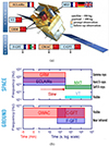 |
Fig. 1. The SVOM mission. (a) Outline of the SVOM mission, including the space and ground instruments. (b) Time and energy coverage of the instruments in the SVOM mission. |
The attitude of SVOM will be pre-defined, so that for most of the year the optical axis of the instruments will be pointed at an offset angle of 45° from the anti-solar direction. Likewise, it will include periods of avoidance of Sco X-1 and the Galactic plane within the ECLAIRs field of view (FoV). The pointing law has been optimised to ensure that most GRBs detected by SVOM could be followed-up by large ground-based facilities to increase the number of GRBs with a measured redshift (Wei et al. 2016). Due to this pointing strategy, the Earth will transit through the ECLAIRs FOV, inducing significant modulation of the background count rate.
ECLAIRs is the wide-field (∼2 sr) coded-mask trigger camera of SVOM. It is tasked with autonomously performing the detection and first localisation of a transient event with a typical accuracy better than 13′ at a 90% confidence level. The instrument consists of a pixelated array of 80 × 80, 4 × 4 mm2, and 1 mm thick Schottky-type CdTe detectors totaling a geometrical area of ∼950 cm2 (Remoué et al. 2010; Lacombe et al. 2013; Godet et al. 2022). A passive shield made of layers of lead and copper surrounds the detection plane to limit the background level. A coded-mask (see Fig. 2) with a ∼40% transparency below 80 keV is placed 46 cm above the detector plane. The mask pattern consists of blocking and transparent elements to the high-energy radiation. It was designed so that its projection on the detection plane (called a shadowgram) is unique for a given source position within the ECLAIRs FOV. Therefore, sky images can be reconstructed via deconvolution of the shadowgram with the mask pattern, enabling the localisation of sources in the FOV. The ECLAIRs FOV is thus divided into 199 × 199 sky pixels.
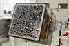 |
Fig. 2. ECLAIRs flight model: view of the coded mask. |
The level of coding of the incoming source photons can vary depending on the position of the source within the FOV. When the source is located within the fully coded region of the FoV (fcFoV, 0.15 sr), the source illuminates all of the plane modulated by the mask. Conversely, when the source is located within the partially coded region of the FoV (fcFov), only a subset of the pixels are able to receive photons from the source. ECLAIRs works in photon counting mode, that is, the readout electronics encode for each detected event its position on the plane, the detection time, and the deposited energy.
In order to optimise ECLAIRs detection sensitivity to certain populations of high-energy transients, including high-z GRBs, X-ray flashes, and X-ray rich GRBs, ECLAIRs presents a low-energy threshold (hereafter Elow) of 4 keV (Godet et al. 2022). This value is lower than that of previous similar high-energy instrumentation such as Swift/BAT. The key advantage of this low Elow value is that it increases the likelihood of detecting transients that may peak in the hard X-ray range. This is the case of high-z GRBs since their measured emission in the observer’s frame would peak at lower energy than if they were placed at lower-z values, due to the reddening of the source emission. Furthermore, this Elow value could aid in constraining the low-energy segment of the prompt emission spectra, contributing to a more precise understanding of the physics driving the prompt emission.
The ECLAIRs data processing unit makes use of the recorded events to search in near real time for the appearance of new transients within the instrument FOV (Dagoneau 2020). To do so, ECLAIRs uses two trigger algorithms (see Schanne et al. 2013, for a detailed description), envisioned for transients of different natures, mainly relative to their duration and intensity. On short timescales, a count-rate trigger monitors count-rate excesses over four energy bands between 4 and 120 keV, nine detector zones (see Fig. 3 of Schanne et al. 2013), and 12 timescales ranging from 10 ms to 20.48 s. When the count rate exceeds a threshold in signal-to-noise ratio (S/N; which depends on the energy band, timescale, and zone considered), a sky image is built on the corresponding timescale and energy intervals. The trigger is then validated if a significant excess (e.g. S/N ≥ 6.5) is found in the sky image. Longer transients are searched for via an image trigger on sky images built every 20.48 s and stacked together on timescales up to ∼20 min (Dagoneau et al. 2018). The threshold used to validate an excess is also S/N ≥ 6.5.
After the detection and localisation of a high-energy transient with ECLAIRs, alert messages carrying essential information on the detected events are broadcast to a network of very high-frequency (VHF) antennas spread around the Earth in the inter-tropical zone. In parallel, the satellite autonomously slews if possible, typically in less than five minutes, towards the source position provided by ECLAIRs. This enables the follow-up by the onboard narrow-field instruments MXT and VT to sample the afterglow emission and to sequentially refine the source localisation. The wide-field GRM instrument extends the spectral coverage of the GRB prompt emission, up to ∼5 MeV. This enables the constraint of the spectral properties of the prompt emission and therefore the measurement of the energetics of the detected GRBs if the source redshift is measured. In parallel, the SVOM robotic ground telescopes are also able to re-point towards the obtained sky position to enhance the follow-up.
3. Sample
3.1. Sample selection
The sample of GRBs selected for the analysis was built on previous prompt emission detection by Swift/BAT and Fermi/GBM (Meegan et al. 2009; Goldstein et al. 2012). For this, we selected all the GRBs with a redshift measurement, up to GRB 200829A, from the Swift GRB website1. Additionally, some high-z GRBs also detected by Swift but whose redshift information does not appear on this table were added based on the literature: GRB 050502 (Schulze et al. 2015, photometric z = 5.2 ± 0.3), GRB 071025 (Fynbo et al. 2009, spectroscopic z ≈ 5.2, estimate), GRB 080129 (Greiner et al. 2009, spectroscopic z = 4.349), GRB 120923A (Tanvir et al. 2018, spectroscopic z = 7.8), GRB 090429B (Cucchiara et al. 2011, photometric z = 9.4).
In the cases where the redshift measurement is inaccurate (denoted as tentative; see Lien et al. 2016), where two or more discordant values are given, or where only an upper limit or range is available, the GRBs were not included. This reduced the sample from 385 to 368 GRBs. When two or more close redshift measurements are given for the same GRB the mean value was taken, unless both spectroscopic and photometric measurements are given, in which case the spectroscopic were kept due to their better accuracy. The Gamma-ray Coordinates Network (GCN) circulars archive2 was used to complement the Swift GRB redshift information when needed. More specific Swift/BAT data, such as spectral parameters, burst duration parameters, and their 90% confidence uncertainties, were retrieved from the Third Swift BAT GRB Catalog (Lien et al. 2016)3.
The Swift/BAT data were complemented, when available, with Fermi/GBM data from the Fourth Fermi GBM Gamma-Ray Burst Catalog4 (von Kienlin et al. 2020), since it provides more constrained spectra derived from a wider energy range (10−1000 keV), and thus is useful to consider for the purpose of redshifting GRBs. The spectra for Swift/BAT GRBs (15−350 keV) are typically described by a power law (PL) or a cut-off law (CPL; see Lien et al. 2016), while two additional models are used for Fermi/GBM (see Goldstein et al. 2012): the Band function (Band et al. 1993) and the smoothly broken power law (SBPL; Kaneko et al. 2006). In any case, the spectral data obtained from these catalogues and used in the present study correspond to time-integrated (or time-averaged) spectral data. In Appendix B we compare the results of the analysis for three GRBs for which we used time-resolved spectral data from Yu et al. (2016). This comparison shows that the qualitative impact of this simplification on the results is not significant.
When combining the two catalogues and to ensure that the detection from both instruments correspond to the same burst, the catalogues were merged based on the trigger time (within a margin of 300 s) and the measured position (within a margin of 2′). All GRBs with z < 3 that were not detected by both instruments were filtered out. However, no filtering was applied to GRBs above this redshift in order to maintain all high-z GRBs from both catalogues.
The sample was further filtered by dropping those GRBs that lack complete spectral information from any of the catalogues. Finally, the sample contains 162 GRBs, 20 of which have a less accurate redshift measurement (obtained via a photometric measurement or denoted as an estimation in the Swift/BAT catalogue). Appendix A contains a table with all GRBs in the sample. The light curves used for our simulations are the 15−350 keV background-subtracted 64 ms binned T100 light curves from the Third Swift/BAT GRB Catalog (Lien et al. 2016).
To ensure compatibility between the spectral models derived from Fermi/GBM and the light curves used in the simulations, the normalisation factors for these models were recomputed. This normalisation factor, denoted as A, was computed as
where FE1 → E2 represents the total measured GRB photon flux over the energy range E1–E2, while f1(E) is the photon flux at energy E computed with A = 1 (see Sect. 4 of Goldstein et al. 2012 for the details about the computation of f(E) for each model). The primary interest in using Fermi/GBM data lies in the spectral shape information, which is contained in f1(E). Re-computing the normalisation factor allows us to obtain a spectral model consistent with F15 → 350, corresponding to the energy range of the Swift/BAT light curves used. This is important for the first step of the simulations, which is the generation of the photon lists at various redshift values (see Sect. 4.1).
3.2. Sample properties
The GRB duration (i.e. the duration of the prompt emission) is commonly described via the T90 parameter. This parameter indicates the duration of the time interval over which 90% (i.e. from 5% to 95%) of the burst counts are recorded within the instrument’s energy range. Although it is measured in the observer frame ( ), its rest-frame value,
  , can be computed as
  .
.
The rest-frame T90 values are plotted against the measured redshift in Fig. 3 for all GRBs in the sample. The errors are quoted at a 90% confidence level. The solid line represents the  rolling average, computed for z-bins of unity size and spaced by 0.4 (not shown for z > 5 due to the sparsity of data). The data points are colour-coded based on the rest-frame isotropic energy, Eiso, which is computed as follows (see e.g. Zitouni et al. 2014; Atteia et al. 2017; Arcier et al. 2020):
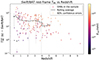 |
Fig. 3. Rest-frame T90 as a function of redshift for the GRBs in the sample, colour-coded based on the bursts Eiso. The solid line corresponds to the |

Here SE1 → E2 is the measured fluence over the energy range E1–E2 (in keV) given in the catalogues. The spectral model parameters used here to compute the photon flux f(E), including the normalisation factor, were those given in the corresponding catalogues. The ratio of integrals is the k-correction factor (Bloom et al. 2001), and extrapolates the fluence to a common energy range from 1 keV to 10 MeV. The cosmological parameters used for computing the luminosity distance, DL, are those from the Planck Collaboration: ΩM = 0.315 ± 0.007, ΩL = 0.685 ± 0.007, and H0 = 67.4 ± 0.5 km s−1 Mpc−1 (Aghanim et al. 2018). The speed of light constant in vacuum is denoted by c.
The sparsity of the z ≳ 6 GRB sample (see Fig. 3) may hinder the identification of the intrinsic properties for this population of GRBs. However, most GRBs with z ≳ 6 present rather small  . We note that the
  moving mean, depicted with a solid line, decreases with redshift. Investigating the reasons behind this trend may help to decipher to what extent this is due to instrumental biases.
4. Method
4.1. Simulations
We simulated the detection by ECLAIRs of the GRBs in the sample using tools developed within the SVOM collaboration, similarly to what was done by Arcier (2022). A flowchart showing the different steps of these simulations is displayed in Fig. 4. The green arrows represent the input to each tool (blue boxes), while the orange arrows represent their outputs. The dashed green arrows represent inputs that are fixed for all the simulations.
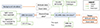 |
Fig. 4. Flowchart of the simulation structure. The three simulator tools used in the analysis are shown as the blue bricks. This process is parallelised for all simulated GRBs, sky positions, and redshift values. |
Firstly, the expected high-energy background along the SVOM orbit is estimated via dynamical background simulations that consider the evolution of orbital parameters. It relies on a particle interaction recycling approach (PIRA) based on a pre-computed database of particle–instrument interactions (Mate et al. 2019). It accounts for the statistical fluctuations on the counts. The dominant background contribution is the cosmic X-ray background (CXB; Churazov et al. 2007). The reflection of CXB photons on the Earth’s atmosphere and the Earth’s albedo, produced by the interaction of cosmic rays with the Earth’s atmosphere (Sazonov et al. 2007), are additional components that can dominate the background counts when the Earth is passing through the instrument’s FOV. Figure 5 illustrates the 4−120 keV and 5.12 s binned background light curve for one orbit showing the background count-rate modulation caused by Earth’s transit.
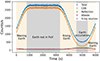 |
Fig. 5. Count-rate evolution of the background measured by ECLAIRs for a standard SVOM orbit, over the 4−120 keV energy range and with a binning of 5.12 s. The contribution of the main background components are displayed in different colours. |
The GRB Simulator (Antier-Farfar 2016) was used to build the list of photons emitted by each GRB, with their corresponding time and energy, hereafter called photon count data. It takes as inputs the light curves and the spectral models from each GRB in the sample. It translates the source spectrum from its observed energy range into the SVOM/ECLAIRs range and normalises the light curves in counts to recover the fluence measured in the ECLAIRs energy range. This tool allowed us to simulate GRBs at redshift values (zsim) higher than their measured values (zmeas) by taking into account cosmological effects such as time dilation, photon flux dimming, and energy shift.
Finally, the ECLAIRs data simulator (Mate 2021) tool allowed us to place the GRBs anywhere along the orbit and in any position of the sky. It is a ray-tracing software that propagates photons one by one through ECLAIRs coded mask. The ray-tracing process considers the energy redistribution due to the transparency of the mask and the detector’s efficiency, in relation to the energy of the incident photons. This tool folds the light curves from the photon count data with the SVOM/ECLAIRs ancillary response file (ARF) and redistribution matrix file (RMF; see diagram in Fig. 4). These response files (Yassine et al., in prep.) describe the on-axis detection efficiency (i.e. for sources in the centre of the FOV). In the ray-tracing process, the mask response for off-axis sources is considered by applying an efficiency geometrical factor, denoted as Oi, j, contingent on the sky pixel (i, j) of the incoming photons. This factor can be regarded as a normalisation term of the curve that describes the effective area as a function of the energy given by the ARF. Figure 6 provides an illustration of the Oi, j values for the pixels along the diagonal and horizontal cuts of the FOV, where θ is the angle between the source direction and the perpendicular to the detector plane (x-axis). Pixels along the diagonal cut have i = j, while pixels along the horizontal cut have i = 100 (see Fig. 7 to visualise the pixel positions). The extent of the fcFoV pixels with respect to θ is indicated for both cuts in their respective colours. At low θ values, corresponding to fully coded detections, the Oi, j factor is only described by a cos(θ) component. At larger θ values, the coding fraction dominates Oi, j, illustrating how the detection efficiency is diminished in the pcFoV.
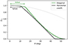 |
Fig. 6. Mask response as a function of the source direction, for the pixels along the diagonal (green) and horizontal (black) cuts of the FOV. |
The output of this tool is composed of the attitude data for the simulated orbit and a photon list with the corresponding time, energy, and position of incidence on the detector plane, hereafter called the event data. The contribution of known X-ray sources within the ECLAIRs FoV (Dagoneau et al. 2021) was also added to the event data along the orbit using this tool. Although some sources can have a significant contribution within the ECLAIRs energy range, the standard orbit with extragalactic pointing considered in this work prevents strong sources within the FOV most of the time.
4.2. Simulation set-up
All GRBs were simulated from zmeas up to zsim = 15 by steps of 0.5 in z. For instance, a GRB with zmeas = 4.3 would be simulated at zsim = 4.3, 4.5, 5, …, 15. The choice of this redshift range, extending up to 15, was made to investigate how ECLAIRs would detect GRBs at these remarkable distances, assuming a GRB population similar to those observed at lower redshifts. This decision is also relevant considering the concurrent operation of the SVOM mission and the James Webb Space Telescope, which detected several candidate galaxies at z > 10 during its first year in operation (e.g. Robertson et al. 2023). All the simulations were performed on the “flat” part of the background (i.e. when the Earth is not within ECLAIRs FOV; see Fig. 5).
The analysis was firstly carried out for GRBs within the fcFoV (i.e. within the central 20 × 20 sky-pixels, ∼575 deg2), to serve as a reference. One hundred trials were run for each simulation case with randomised positions and epochs within the above constraints to account for noise and source fluctuations. This also provided us with a measure of dispersion on the reconstructed GRB properties for each simulation case. A second analysis was performed with the GRBs placed in both the pcFoV and the fcFoV. A grid of 100 positions, separated by ten sky pixels, in one quarter of the FOV was used as a reference to extrapolate the values to the rest of the FOV. This allowed us to compute the fraction of the FOV in which a GRB at a certain redshift can be detected.
Figure 7 shows the positions within the FoV selected for both analyses. The blue points represent the positions used for the fcFoV analysis, while the red points represent the grid of 100 positions for the analysis in all the FOV. The grey-shaded region shows the central 181 × 181 sky pixels within the FoV for which the results of the latter analysis are extrapolated.
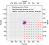 |
Fig. 7. Representation of the positions within the FOV used in each simulation case. The grey-shaded region represents the part of the FoV for which the results of analysis in all the FoV are extrapolated. |
4.3. Signal-to-noise ratio computation
The event data output from these simulations were used to compute the count and image S/Ns, applying a suitable version of the count-rate trigger algorithm (Schanne et al. 2013) presented in Sect. 2. Similarly to the flight algorithm, the count S/N (cS/N) was computed for 12 timescales exponentially spaced with base 2 from 10 ms to 20.48 s, four energy bands (4−120, 4−25, 15−50, 25−120 keV) and nine detector zones. For each of these possible configurations, the light curve was binned with the corresponding timescale and the cS/N was computed for each time bin. It was computed as  , where CGRB corresponds to the counts associated with the GRB, and Cbkg to the background counts. The count rate measured over an interval of three minutes before the GRB trigger time was linearly fitted to estimate the background level. This was then extrapolated to the time of interest (i.e. when the GRB occurred) to compute Cbkg. Then CGRB was computed as the difference between the total counts and Cbkg.
For each possible configuration the time bin with the largest cS/N value was chosen, and then the best cS/N of all those configurations was selected. This computation was also performed by shifting the time interval over which the cS/N was computed by half the width of the time bins, thus changing the binning. This difference in binning accounts for possible better cS/N values. Then, a sky image was reconstructed from the counts received within the energy band and time bin associated with the best cS/N. If the transient was localised in this image with a significance exceeding a pre-set image S/N (iS/N) threshold of 6.5, it was considered a successful detection. The onboard algorithm is slightly different in the sense that it selects all the excesses on the counts above a cS/N threshold and reconstructs the corresponding sky images to search for iS/N values above the iS/N threshold. Here we just reconstructed the sky image and derived the iS/N for the best cS/N configuration over the time bins considered, assuming it would correspond to the highest iS/N, to minimise the computational cost of the simulations.
To assess whether a GRB could be detected at a certain redshift within the fcFoV, we used the median of the iS/N values obtained in the 100 trials, hereafter iS/Nmed. The redshift horizon for a GRB, zhor, was computed as the maximum redshift at which the GRB is detectable with iS/Nmed ≥ 6.5.
Regarding the fraction of the FOV over which a GRB is detectable, we computed the iS/N values for 100 sky pixels within one quarter of the ECLAIRs FOV, including fcFoV and pcFoV (see Sect. 4.2 and Fig. 7). These values, after extrapolation to the other three quarters, were interpolated to derive the expected iS/N value for each of the other sky pixels in between. Because sky pixels do not all cover the same portion of the FOV, it was necessary to apply weights of FOV coverage by pixel in order to estimate the fraction of the complete FOV with iS/N ≥ 6.5.
4.4. GRB duration measurements
When a GRB is successfully detected, we derived its duration,  , using the standard battblocks5 tool, from the HEASOFT v2.17 software. It applies a Bayesian blocks algorithm (see Scargle 1998) for segmenting time-variable data into intervals based on Bayesian analysis. Specifically, we input the 80 ms binned light curve over the whole 4−120 keV energy band. This tool is commonly employed for ground analyses of Swift/BAT data (e.g. Littlejohns et al. 2013; Zhang et al. 2013; Lien et al. 2016; Moss et al. 2022). The duration uncertainties are computed using ±1σ confidence bands around the cumulative light curve. Since we computed the duration for 100 trials and we took the median, we also computed the 90% confidence intervals for the median based on the values obtained in the trials.
The comparison of the  median values computed for each GRB in the sample at zmeas within the ECLAIRs fcFoV, with the measured values from Swift/BAT revealed a potential bias in the analysis. It is worth noting, however, that this bias should not affect qualitatively the results presented in this paper (see Appendix C for more details).
5. Results
As output of the simulations, for each GRB and zsim, we obtained the iS/Nmed within the fcFoV as well as the fraction of the FOV over which the GRB would be detectable. The maximum redshift horizon, zhor, was also obtained for each GRB, based on the iS/Nmed within the fcFoV. For those zsim values ≤zhor, the corresponding T90 values were derived. Table E.1 summarises some of these results for each GRB in the sample.
First, a subset of GRBs is chosen to present the results individually in Sect. 5.1. The choice of these GRBs is motivated by the shape and evolution of their light curves with increasing redshift. If we divide the GRB sample in different classes based on their T90 evolution with redshift, these GRBs can be representative of these diverse classes (see Sect. 5.5). The results obtained for the whole sample are presented in the following sections.
5.1. Case studies
Together with the individual description of each GRB chosen for the case study, some plots are shown with the results of the three GRBs presented in this section. Figure 8 shows the light curves of these GRBs at different zsim values, in one of the trials within the fcFoV. The obtained  intervals for that trial are depicted with a grey-shaded band and the corresponding values are written at the top of each plot. While the light curves and values shown in this figure correspond to one trial, the results mentioned in the text correspond to the median of 100 trials. Figure 9 illustrates the evolution of the T90 value in the source rest frame (
 ) as a function of zsim for the three GRBs. The curves end at their redshift horizon, zhor. The median error bars correspond to those obtained with battblocks, which are the error values reported hereafter. The 90% confidence interval of the
  median value was computed for comparison, and is represented in this figure with a shaded region.
-
GRB 140311A was detected by Swift/BAT yielding a
 value of 71.4 ± 9.5 s within the 15−350 keV band. Its 15−150 keV time-averaged spectrum was best fitted by a PL with an index of 1.67. Its light curve shows a weak peak of about 10 s around the trigger time, and another weak peak of about 20 s starting ∼40 s after the trigger (Krimm et al. 2014). There is no detection of this GRB by Fermi/GBM. Gemini-south (Tanvir et al. 2014), Gemini North (D’Avanzo et al. 2014), and the Nordic Observatory Telescope (Chornock et al. 2014) observations found consistent spectroscopic values of redshift at zmeas ∼ 4.95. Our simulations yield that ECLAIRs would detect this GRB within its fcFoV at its zmeas value with an iS/Nmed ∼ 27 and a derived
  s. The simulations at higher redshifts within ECLAIRs fcFoV show that it could be detected up to zhor ∼ 10.5, with iS/Nmed ∼ 6.9. Regarding the analysis over the entire FOV, GRB 140311A could be detected at its zmeas within ∼81% of the FOV. This fraction decreases to below 50% at zsim ∼ 8.5. As seen in panel a of Fig. 8, the burst signature on the light curve is stretched in time and dimmed in intensity with increasing zsim due to cosmological dilation. The derived
  value increases accordingly over all the zsim values at which it is detected. As seen in Fig. 9, the
  values for this GRB, in orange, stay relatively constant for all zsim.
 -
GRB 090424 was a multi-peaked GRB first detected by Swift/BAT, with
 s. Its light curve shows very bright peaks during the first 5−6 s trailing off into smaller peaks at around 8 s, 15 s, and 50 s after the trigger (Cannizzo et al. 2009). The coincident Fermi/GBM detection provided us with a Band function as the best-fit spectral model, with
  keV (Connaughton 2009). The spectroscopic redshift measured for this GRB is relatively low at 0.544 (Gemini-South, Chornock et al. 2009; William Herschel Telescope, Wiersema et al. 2009). According to our simulations, this GRB could be detected by ECLAIRs at its zmeas within its fcFoV with iS/Nmed ∼ 237, and a
  duration of 98 ± 4.56 s. Its redshift horizon is zhor ∼ 8.5, with iS/Nmed ∼ 7.3. The proximity of this GRB, together with its brightness make it detectable virtually anywhere within the FOV at its zmeas value. However, the detectable fraction of the FoV rapidly drops with increasing redshift. The evolution of the light curve with zsim is shown in panel b of Fig. 8. The y-axes in all adjacent subplots are fixed in order to easily track the light curve evolution. In consequence, the burst signature on the right subplot at zsim = 8.5, yet detectable by the trigger, is not easily distinguishable by eye. The evolution of the light curve with zsim is consistent with the effect of cosmological dilation. However, as opposed to the trend seen for the aforementioned GRB, the
  value rapidly decreases as the secondary peaks and tail of the emission are buried within the background noise. Figure 9 reveals how the
  value decreases during the first zsim, as this low-flux emission is lost. Above zsim ∼ 3, the
  value stays roughly constant up to zhor.
 -
GRB 090516A was detected by Swift/BAT with
 s, later refined in the catalogue to
  s. The time averaged Swift/BAT spectrum is best fit by a PL with an index of 1.84 (Rowlinson et al. 2009). The coincident Fermi/GBM detection (McBreen 2009) provided us with a CPL function as the best-fit spectral model. The light curve consists of about five overlapping pulses lasting at least 150 s. A redshift value of 4.1 was measured spectroscopically and photometrically using the Very Large Telescope (de Ugarte Postigo et al. 2009), the Gamma-Ray Burst Optical/Near-Infrared Detector (Rossi et al. 2009), and the Stardome Observatory (Christie et al. 2009). The simulations within the ECLAIRs fcFoV at zmeas yield iS/Nmed ∼ 66 and
  s. This GRB is intrinsically bright enough that it could be detected at z ≳ 15 within the fcFoV. Similarly to GRB 090424, the decrease in
  as a function of zsim is evident but gradual over several zsim values (see Fig. 9). At zmeas the GRB is detectable over ∼98% of the FOV. The detectable fraction of the FOV remains above 60% up to zsim ∼ 10, and rapidly drops below 30% beyond zsim ∼ 13.
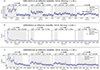 |
Fig. 8. Evolution of the retrieved 4−120 keV light curves at different zsim for a specific position within the fcFoV, for the three GRBs described as case studies. GRB 140311A, GRB 090424, and GRB 090516A are shown in panels a–c respectively. For better visualisation, different binning is used for each GRB, both axes are fixed for all plots in the same panel, and the y-axis is shown in logarithmic scale in panels b and c. The obtained T90 interval is shown with a grey shaded band on each light curve, and the corresponding values written on top, if the detection was successful. These light curves and values correspond to one trial, and hence they may differ from the values given in the text, which correspond to the median of 100 trials. |
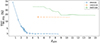 |
Fig. 9. Evolution of |

5.2. Sample detectability within the fcFoV
We have shown as an example three GRBs that could be detected by ECLAIRs up to very high redshifts, higher than any GRB detected so far. However, it is fundamental to check whether these are special cases or if there are more such GRBs in our sample.
We divided our sample into four subsets of ∼40 GRBs, according to their zmeas value, into the following ranges: [0.078–1.33], [1.33–2.86], [2.86–3.83], and [3.83–9.4]. The lowest and highest redshift subsets contain 41 GRBs each, while the two intermediate subsets comprise 40 GRBs each. Figure 10 illustrates the percentage of GRBs detected within the fcFoV for each of these groups plotted as a function of zsim. The number of detected GRBs out of the total number of simulated GRBs within each group is indicated above each bar in the histogram. We recall that GRBs were not simulated at zsim values lower than their corresponding zmeas value. Therefore, the number of GRBs corresponding to the first zsim values for each curve in Fig. 10 might be small, while the percentage is high (except for the lowest-z subset represented by the blue curve where all GRBs have zmeas < 1.5, which is the lowest-zsim).
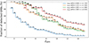 |
Fig. 10. Percentage of detected GRBs within ECLAIRs fcFoV at each simulated redshift for the whole sample, separated into subsets based on their zmeas. The numbers shown at the top of the histogram correspond to the number of detected GRBs in each redshift. |
This figure illustrates that several GRBs could be detected at redshifts higher than 9 or 10, a few even detectable up to zsim ≥ 15. We can also see that the percentage of detected GRBs at a certain redshift is typically smaller for those GRBs which originally had a low redshift. In particular, the percentage of detected GRBs from the lowest-z subset ([0.078–1.33]) is significantly smaller than for the rest of GRBs, at any given redshift. This is due to the lower intrinsic brightness of the GRBs in this subset compared to the other ones.
5.3. Impact of the low-energy threshold
The low value achieved for the low-energy threshold (Elow) of ECLAIRs is a significant characteristic of the instrument. To shed insight into its importance, a comparison was made between the previous analysis results with Elow = 4 keV and an analysis using an Elow of 15 keV, similar to Swift/BAT. The comparison of these two scenarios is illustrated in Figs. 11 and 12 for all the simulation cases (i.e. all GRBs and zsim) within the fcFoV.
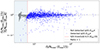 |
Fig. 11. Comparison of the iS/Nmed obtained with Elow values of 15 and 4 keV, for all GRBs, and redshift values simulated within the fcFoV. The blue and grey points represent respectively all successful and not successful detections with Elow = 4 keV. The red vertical line represents the iS/N threshold above which the successful detections with Elow = 15 keV lie. |
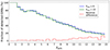 |
Fig. 12. Comparison of the percentage of detected GRBs (iS/Nmed ≥ 6.5) within the fcFoV at each zsim for Elow values of 15 and 4 keV. The dashed red line represents the relative difference between the percentage of both scenarios, with respect to the 4 keV scenario. |
Figure 11 shows the ratio of the iS/Nmed obtained with Elow = 15 keV to that with Elow = 4 keV plotted against the iS/Nmed with Elow = 15 keV. Among the 4157 simulation cases, the ratio is less than unity in 2657 cases (63%), equal to unity in 367 cases (9%), and greater than unity in 1131 cases (22%). Notably, there are 57 cases (blue points on the left of the vertical red line in Fig. 11) for which the detection is successful with Elow = 4 keV, but not with Elow = 15 keV, while only two cases demonstrate successful detection with Elow = 15 keV, but not with Elow = 4 keV.
Figure 12 shows the percentage of GRBs detected within the fcFoV by bins of 0.5 width in redshift, for both scenarios. The relative loss shown by the dashed red line was computed as the difference between the percentage for both scenarios divided by the percentage for the 4 keV scenario. This provides an idea of the extent of the detections that would be lost by setting Elow to 15 keV instead of 4 keV. This relative loss is larger for greater zsim values, escalating from nearly 0% below zsim ∼ 2 up to ∼10% beyond zsim ∼ 10. However, these values should be taken cautiously due to the limited number of GRBs at these high redshifts, rendering the results less statistically robust.
5.4. Detectability outside the fcFoV
Figure 13 shows the evolution with increasing redshift of the fraction of FOV over which a GRB can be detected. The grey curves represent each simulated GRB, while the blue and orange histograms represent the median and mean values, respectively, for redshift bins of width 0.5. At zsim ∼ 5.5, nearly half of the GRBs in the sample (79 GRBs) remain detectable in more than 40% of the FOV. At zsim ∼ 8 and zsim ∼ 10, the number of GRBs would become 42 and 32, respectively.
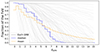 |
Fig. 13. Fraction of the FoV with successful detection (iS/N ≥ 6.5) plotted against zsim for each GRB in the sample (grey curves). The median and mean values for bins of 0.5 width in redshift are shown in blue and orange, respectively. |
At zsim > 7.5, more than half of the GRBs exhibit an almost zero detectable fraction of the FOV, which is consistent with median value observed beyond this redshift range (see Fig. 13). However, a subset of bright GRBs remains detectable within a large fraction of the FOV at very high redshifts (e.g. 20 GRBs are detectable within more than 0.4 of the FOV fraction above zsim ∼ 12). This explains the mean value diverging from the median value above redshift 6. Consistently with the results over the fcFoV, the GRBs detectable up to high redshift values are mostly GRBs not contained within the lowest redshift bin in our sample [0.078−1.33], but equally distributed within the other redshift bins.
5.5. Sample T90 evolution with redshift
The evolution with zsim of  normalised by the derived
  value at zmeas, is depicted for the whole sample in the left panel of Fig. 14. The right panel shows only the GRBs from the lowest-z and highest-z subsets, for clarity. The plots analogous to Fig. 9 (i.e. without normalisation) by subsets of the entire sample can be found in Appendix D.
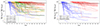 |
Fig. 14. Evolution of |

Each curve in Fig. 14 represents the evolution of a given GRB, colour-coded according to the subset to which it belongs. The black horizontal line represents the threshold value used to classify the GRBs based on their T90 evolution with redshift (see below).
Many GRBs exhibit a behaviour similar to GRB 090424 and GRB 090516A, where a portion of the low-flux emission is buried into the background noise above a certain zsim, resulting in a noticeable decrease in the derived  value. Some of these GRBs display an abrupt decrease in
  at a specific redshift, followed by a plateau of relatively constant
  , as for GRB 090424, while others exhibit a more gradual or steady decrease, similar to GRB 090516A.
On the contrary, many other GRBs maintain a relatively constant  value across all zsim values up to their zhor, indicating that the majority of their emission remains above the background noise level. GRB 060927 and GRB 120521C, which belong to the highest-z bin, are special cases as they exhibit this behaviour, but feature a zhor ≳ 15. Therefore, it is possible that their
  value would decrease at higher redshift values, once their low-flux emission is lost.
GRBs were categorised into two groups based on the ratio of  at zhor to that at zmeas:
  . This ratio provides insight into the extent of the
  decrease between the first and last simulated redshift values. A threshold value of 0.7 (i.e. a decrease of 30%; see Fig. 14) was used to allocate the GRBs into these two groups. This value was chosen based on the distribution of the ratio values for the whole sample. GRBs with a ratio below 0.7 were allocated in the Decrease group indicating a significant decrease in
  , while those with higher ratio were allocated in the Uniform group indicating a rather constant
  value. Within the Decrease class, GRBs were further divided into those with an abrupt decrease (≳25% between two consecutive zsim) and those with a gradual decrease. GRBs not detected above their zmeas were not categorised in any group (N/C).
Table 1 presents the number of GRBs allocated to each class, categorised by the subsets based on their zmeas in the sample. The table also indicates the number of GRBs in the Uniform class with zhor ≳ 15.
GRBs categorised according to their  decrease with zsim.
There is an increasing trend in the number of GRBs categorised as Uniform as the zmeas value increases, while the subsets with lower zmeas contain a higher proportion of GRBs in the Decrease class. Most of those categorised as decreasing show an abrupt decrease between two consecutive zsim, rather than a gradual decrease.
This T90 bias may lead to significantly divergent measurements at different redshift values, dropping to less than 5% of the value at zmeas for certain GRBs. A comparable loss of measured GRB counts arising from this T90 reduction could lead to a more pronounced impact on the measured properties (e.g. luminosity) of some bursts. However, upon a preliminary examination of the count loss within the measured T90 interval, it appears to be generally less substantial than the reduction in T90.
6. Discussion
In this section we discuss the main findings of this study, outlined in Sect. 5, after having simulated a carefully selected sample of GRBs (see Sect. 3), emulating a realistic detection scenario by ECLAIRs, at different zsim values, equal to and higher than their zmeas value (see Sect. 4). Firstly, we discuss the main findings in terms of detection capabilities of ECLAIRs, and then we discuss the instrumental effects on the reconstruction of source measured properties, such as GRB duration. While the majority of GRBs are spatially more likely to lie within the pcFoV, a significant part of the analysis presented in this study corresponds to the simulations within the fcFoV to serve as a reference.
The results of the simulations outlined in Sect. 5.2 suggest that ECLAIRs has the potential to detect GRBs at extremely high redshifts (z > 15), significantly surpassing the redshift values of the highest-z GRBs known to date (z ≈ 9.4). The ability to detect these high-z GRBs is particularly prominent when the GRBs are located within the fcFoV, which represents only a ∼7.24% of the instrument’s FOV. However, even within the pcFoV (see Sect. 5.4), where more GRBs would lie based on spatial likelihood but where the detection is more challenging, a substantial number of bright GRBs, with Eiso ≳ 1053 erg, can still be detected at very high-z values. Out of the 162 GRBs in the sample, 14 GRBs could be detected within more than 50% of the FOV at z ∼ 15 and 47 GRBs at z ∼ 9. On the other hand, the diminishing median value of the detectable fraction of the FOV beyond z = 7 (Fig. 13) suggests that standard GRBs are less likely to be detected outside the fcFoV at these redshift ranges.
The low-energy threshold (Elow) of the ECLAIRs energy range, which extends down to 4 keV, is one of the contributing factors to the good high-z GRB detection performance obtained from our simulations. Setting the low-energy threshold, Elow to 15 keV instead, would deteriorate its detection capabilities in more cases than it would improve it. This is more significant at high-z values, reaching ≳10% loss at zsim > 10. It is therefore important to set the trigger Elow threshold as close as possible to that of the camera (i.e. 4 keV). To do so, specific care in the flight calibration should be devoted during the SVOM commissioning phase. With this capability, ECLAIRs is expected to contribute to slightly augmenting the number of detected GRBs at high redshift.
Demonstrating that ECLAIRs will be able to detect GRBs possibly with z > 10 does not mean that such GRBs will be identified as such, as there is a step to go from detection to identification, which is challenging. Accurate redshift measurements for high-z GRBs present challenges as they require near-infrared observations of the afterglow, which rely upon follow-up observations by other instruments. The sensitivity and availability of multi-wavelength instruments for the follow-up are therefore limiting conditions to obtain the redshift measurements. These limitations could play a role in the scarcity of known high-z GRBs in the current sample, thus contributing to the notable disparity in detectability at high-z between the simulations and the current GRB sample. The detection of the afterglow is therefore crucial for increasing the sample of known high-z GRBs. In order to address this challenge, and to fill the gap between the detection and the identification of GRBs, the SVOM collaboration have put in place a dedicated pointing strategy (i.e. quasi anti-solar pointing) coupled with a strong space and ground synergy to enhance the GRB follow-up on ground promptly and efficiently (see Wei et al. 2016; Atteia et al. 2022).
We recall that we used a sample of already observed GRBs to perform our study, to stay as close to reality as possible, since there are no spectral nor temporal templates of GRB emission accounting for the diversity of their observational properties. We shall therefore face that the instruments that have observed these GRBs have likely imprinted some instrumental biases on the source intrinsic properties. For instance, some low-flux temporal structures may have disappeared within the noise due to the observing conditions (e.g. angle of incidence; Moss et al. 2022) and/or may have fallen outside of the energy range of the instruments. Figure 10, considering the GRBs in the various redshift ranges subsets, clearly evidences the instrumental biases imprinted on the high-z GRB sample. The lower detectability of the GRBs in the lowest-z subset (zmeas < 1.33, blue curve), is due to their lower intrinsic brightness. This selection effect is also shown in the analysis of the T90 evolution with redshift, discussed below.
In this study, we estimated the detectability using the count-rate trigger with the same threshold as the onboard algorithm. Some additional bursts may be found using the onboard image trigger, or using the on-ground ECLAIRs offline trigger featuring complementary algorithms or applying lower threshold values for the count-rate trigger. In particular, considering that the emission of high-z GRBs in the observer’s frame may be significantly stretched, it would be beneficial to use the image trigger, which is well suited to detect GRBs featuring a very long emission (Dagoneau et al. 2020). Therefore, one could expect a larger fraction of GRBs detected with the image trigger than with the count-rate trigger, consistently with Swift/BAT (Lien et al. 2016, Fig. 22). However, the T90 bias presented in Sect. 5.5 might counteract this effect reducing the image trigger performance as the GRB emission that stands above the noise would be shorter. Further analyses need to be done in order to address this.
On the other hand, additional ECLAIRs instrumental effects (see e.g. Arcier 2022), the evolution of the background on the orbit and over time, alongside the efficiency of background suppression on actual data (on the ground and on board) may reduce the overall efficiency in detecting this GRB population, compared to the simulations. Likewise, even if significant effort has been put into making a realistic background simulator, accurately simulating the background is challenging, thus it could be underestimated in our simulations. Therefore, the results of these simulations should be interpreted cautiously as they might lean towards an overly optimistic outlook. The smaller effective area of ECLAIRs compared to that of Swift/BAT should typically result in an overall lower detection efficiency. It is worth emphasising that these results are not indicative of the expected rate of identified high-z GRBs with ECLAIRs, nor are they intended for direct comparison with observational results from past missions. Rather, their purpose is to estimate ECLAIRs’ potential to detect GRBs at high redshift values, while considering the aforementioned caveats, and recalling that the detection of a GRB does not imply the identification of their redshift. Moreover, the evolution of GRB progenitor populations with redshift cannot be ruled out. Although the current study does not directly address this aspect, it aims to provide further insight by highlighting the potential biases involved in the detection and identification of high-z GRBs.
In Sect. 5.5, we showed the presence of detection biases in the GRB duration measurements as a function of redshift. For some GRBs, such as GRB 090424 and GRB 090516A, the measured value of  decreases with increasing redshift (categorised as decreasing) because a part of the low-flux emission is lost within the noise. On the other hand, the effect of this bias is not evident in other bursts like GRB 140311A, which display an almost non-decreasing
  value (categorised as uniform).
GRBs with a lower zmeas are more likely to belong to the former category, while those with a higher zmeas are more likely to belong to the latter (see Fig. 14 and Table 1). This is mainly because the low-flux emission of those with higher zmeas may have been lost for the detection by Swift/BAT, and thus not present in the light curves used as input of our simulations.
Similarly to many other GRBs in the Decreasing T90
class, the  value for GRB 090424 reaches a plateau (at zsim > 3) after an abrupt decrease (see Fig. 9). This plateau resembles the curves exhibited by the GRBs in the Uniform T90
class. It is likely that many GRBs in this class do not show a significant decrease in
value for GRB 090424 reaches a plateau (at zsim > 3) after an abrupt decrease (see Fig. 9). This plateau resembles the curves exhibited by the GRBs in the Uniform T90
class. It is likely that many GRBs in this class do not show a significant decrease in  because the low-flux emission coming from these GRBs was not detected originally by Swift/BAT. If GRB 090424 had been detected at z ∼ 5, as for GRB 140311A, the low-flux emission would probably not have been detected, leading us to put it into the Uniform class since the
  value would have remained constant throughout the simulations.
All of these pieces of evidence show the instrumental bias in the measurement of the GRB duration as a function of their redshift, in agreement with the results from Littlejohns et al. (2013). This effect may partially explain why the measured T90 values of currently known high-z GRBs tend to be lower than expected (see Fig. 3). However, drawing definitive conclusions in this regard is complicated, primarily due to the limited size of the available sample. The bias is highly dependent on the light curve shape, which in turn relies on the intrinsic characteristics of the GRB internal jet physics. Therefore, discerning between scenarios where low-flux emissions remain undetected and those where the entire emission is captured proves to be challenging.
It is important to note that this bias is not specific to the T90 parameter alone, but to the GRB duration in general. One could naively think that the T50 would be less affected by this bias as its interval might not encompass the low-flux emission that is buried in noise at higher redshift values, unlike the T90 interval. However, the results from the simulations indicate that the T50 parameter is also notably affected by this bias.
Such biases may inadvertently lead to erroneous associations, potentially misclassifying core-collapse GRBs with a short measured duration as compact merger progenitor events. One should be cautious in using the GRB duration alone to infer the nature of their progenitors. Likewise, this effect may impact the reconstruction of other source properties. For instance the derived fluence will be affected by the GRB duration, even if the derived flux was not highly impacted, as it is mainly the low-flux emission that is lost within the noise. This can directly impact the derivation of the Eiso value (see Eq. (2)), thus also impacting analyses related to energy and luminosity relations, which can be used as cosmological probes. It is also likely that there will be a lack of useful GRM data for most high-z GRBs. Consequently, we will have to rely on the energy range covered by ECLAIRs to assess the burst energetics. Due to its narrow energy range, similar to that of Swift/BAT, it is likely that our estimates on the prompt emission energetics of high-z GRBs may be biased. Therefore, despite its complexity, it is essential to pursue a comprehensive understanding of the various biases (e.g. ECLAIRs detection, SVOM observing strategy) that will affect the GRB populations observed by SVOM. A similar study, but including the potential detection with GRM could contribute to unravelling these biases.
Swift GRB table, available at https://swift.gsfc.nasa.gov/archive/grb_table/
All GCN circulars available at https://gcn.gsfc.nasa.gov/gcn3_archive.html
The Swift/BAT Catalog available at https://swift.gsfc.nasa.gov/results/batgrbcat/
The Fermi-GBM Catalog available at https://heasarc.gsfc.nasa.gov/W3Browse/fermi/fermigbrst.html
References
- Abbott, B. P., Abbott, R., Abbott, T. D., et al. 2017, ApJ, 848, L12 [Google Scholar]
- Aghanim, N., Akrami, Y., Ashdown, M., et al. 2018, A&A, 641, A6 [Google Scholar]
- Antier-Farfar, S. 2016, PhD Thesis, Université Paris Saclay, France [Google Scholar]
- Arcier, B. 2022, PhD Thesis, Université Paul Sabatier-Toulouse III, France [Google Scholar]
- Arcier, B., Atteia, J. L., Godet, O., et al. 2020, Astrophys. Space Sci., 365, A185 [NASA ADS] [CrossRef] [Google Scholar]
- Atteia, J.-L., Heussaff, V., Dezalay, J.-P., et al. 2017, ApJ, 837, 119 [CrossRef] [Google Scholar]
- Atteia, J.-L., Cordier, B., & Wei, J. 2022, Int. J. Modern Phys. D, 31, 2230008 [NASA ADS] [CrossRef] [Google Scholar]
- Band, D., Matteson, J., Ford, L., et al. 1993, ApJ, 413, 281 [Google Scholar]
- Barthelmy, S. D., Barbier, L. M., Cummings, J. R., et al. 2005, Space Sci. Rev., 120, 143 [Google Scholar]
- Basa, S., Lee, W. H., Dolon, F., et al. 2022, Proc. SPIE, 12182, 602 [Google Scholar]
- Bloom, J. S., Frail, D. A., & Sari, R. 2001, AJ, 121, 2879 [NASA ADS] [CrossRef] [Google Scholar]
- Bromberg, O., Nakar, E., Piran, T., & Sari, R. 2013, ApJ, 764, 179 [NASA ADS] [CrossRef] [Google Scholar]
- Bromm, V., & Loeb, A. 2006, ApJ, 642, 382 [Google Scholar]
- Campana, S., Salvaterra, R., Melandri, A., et al. 2012, MNRAS, 421, 1697 [Google Scholar]
- Cannizzo, J. K., Barthelmy, S. D., Beardmore, A. P., et al. 2009, GRB Coordinates Network, 9223, 1 [NASA ADS] [Google Scholar]
- Chaoul, L., Mousset, V., & Quenouille, G. 2018, 2018 SpaceOps Conference, 2509 [Google Scholar]
- Chornock, R., Perley, D. A., Cenko, S. B., & Bloom, J. S. 2009, GRB Coordinates Network, 9243, 1 [NASA ADS] [Google Scholar]
- Chornock, R., Fox, D. B., Tanvir, N. R., & Berger, E. 2014, GRB Coordinates Network, 15965, 1 [NASA ADS] [Google Scholar]
- Christie, G. W., de Ugarte Postigo, A., & Natusch, T. 2009, GRB Coordinates Network, 9396, 1 [NASA ADS] [Google Scholar]
- Churazov, E., Sunyaev, R., Revnivtsev, M., et al. 2007, A&A, 467, 529 [NASA ADS] [CrossRef] [EDP Sciences] [Google Scholar]
- Connaughton, V. 2009, GRB Coordinates Network, 9230, 1 [NASA ADS] [Google Scholar]
- Corre, D., Basa, S., Klotz, A., et al. 2018, Proc. SPIE, 10705, 565 [Google Scholar]
- Costa, E., Frontera, F., Heise, J., et al. 1997, Nature, 387, 783 [NASA ADS] [CrossRef] [Google Scholar]
- Cucchiara, A., Levan, A. J., Fox, D. B., et al. 2011, ApJ, 736, 7 [Google Scholar]
- Dagoneau, N. 2020, PhD Thesis, Université Paris-Saclay, France [Google Scholar]
- Dagoneau, N., Schanne, S., Gros, A., & Cordier, B. 2018, ArXiv e-prints [arXiv:1810.12052] [Google Scholar]
- Dagoneau, N., Schanne, S., Atteia, J.-L., Götz, D., & Cordier, B. 2020, Exp. Astron., 50, 91 [Google Scholar]
- Dagoneau, N., Schanne, S., Rodriguez, J., Atteia, J.-L., & Cordier, B. 2021, A&A, 645, A18 [NASA ADS] [CrossRef] [EDP Sciences] [Google Scholar]
- Dai, Z., Daigne, F., & Mészáros, P. 2017, Space Sci. Rev., 212, 409 [NASA ADS] [CrossRef] [Google Scholar]
- D’Avanzo, P., D’Elia, V., Piranomonte, S., et al. 2014, GRB Coordinates Network, 15964, 1 [Google Scholar]
- de Ugarte Postigo, A., Gorosabel, J., Malesani, D., Fynbo, J., & Levan, A. J. 2009, GRB Coordinates Network, 9383, 1 [NASA ADS] [Google Scholar]
- Dong, Y., Wu, B., Li, Y., et al. 2009, Sci. China Ser. G: Phys. Mech. Astron., 53, 40 [Google Scholar]
- Eichler, D., Livio, M., Piran, T., & Schramm, D. N. 1989, Nature, 340, 126 [NASA ADS] [CrossRef] [Google Scholar]
- Fan, X., Zou, G., Wei, J., et al. 2020, Int. Soc. Opt. Photon., 11443, 114430Q [Google Scholar]
- Fynbo, J. P. U., Jakobsson, P., Prochaska, J. X., et al. 2009, ApJS, 185, 526 [NASA ADS] [CrossRef] [Google Scholar]
- Galama, T., Vreeswijk, P., Van Paradijs, J., et al. 1999, A&AS, 138, 465 [NASA ADS] [CrossRef] [EDP Sciences] [Google Scholar]
- Gardner, J. P., Mather, J. C., Clampin, M., et al. 2006, Space Sci. Rev., 123, 485 [Google Scholar]
- Gehrels, N. 2004, AIP Conf. Proc., 727, 637 [NASA ADS] [CrossRef] [Google Scholar]
- Gehrels, N., Norris, J., Barthelmy, S., et al. 2006, Nature, 444, 1044 [NASA ADS] [CrossRef] [Google Scholar]
- Godet, O., Sizun, P., Barret, D., et al. 2009, Nucl. Instrum. Meth. Phys. Res. Sect. A, 603, 365 [Google Scholar]
- Godet, O., Nasser, G., Atteia, J. L., et al. 2014, Proc. SPIE, 9144, 914424 [NASA ADS] [CrossRef] [Google Scholar]
- Godet, O., Atteia, J.-L., Amoros, C., et al. 2022, in Space Telescopes and Instrumentation 2022: Ultraviolet to Gamma Ray, eds. J.-W. A. den Herder, S. Nikzad, & K. Nakazawa (SPIE), Int. Soc. Opt. Photon., 12181, 121815O [NASA ADS] [Google Scholar]
- Goldstein, A., Burgess, J. M., Preece, R. D., et al. 2012, ApJS, 199, 19 [Google Scholar]
- Gottlieb, O., Metzger, B. D., Quataert, E., Issa, D., & Foucart, F. 2023, ApJL, 958, 33 [Google Scholar]
- Greiner, J., Krühler, T., McBreen, S., et al. 2009, ApJ, 693, 1912 [NASA ADS] [CrossRef] [Google Scholar]
- Greiner, J., Fox, D. B., Schady, P., et al. 2015, ApJ, 809, 76 [NASA ADS] [CrossRef] [Google Scholar]
- Götz, D., Meuris, A., Pinsard, F., et al. 2016, Proc. SPIE, 9905, 99054L [CrossRef] [Google Scholar]
- Han, X., Xiao, Y., Zhang, P., et al. 2021, PASP, 133, 065001 [NASA ADS] [CrossRef] [Google Scholar]
- Hjorth, J., Sollerman, J., Møller, P., et al. 2003, Nature, 423, 847 [Google Scholar]
- Ivezić, Ž., Kahn, S. M., Tyson, J. A., et al. 2019, ApJ, 873, 111 [Google Scholar]
- Kaneko, Y., Preece, R. D., Briggs, M. S., et al. 2006, ApJ, 166, 298 [NASA ADS] [Google Scholar]
- Klebesadel, R. W., Strong, I. B., & Olson, R. A. 1973, ApJ, 182, L85 [NASA ADS] [CrossRef] [Google Scholar]
- Krimm, H. A., Barthelmy, S. D., Baumgartner, W. H., et al. 2014, GRB Coordinates Network, 15962, 1 [NASA ADS] [Google Scholar]
- Kumar, P., & Zhang, B. 2015, Phys. Rep., 561, 1 [Google Scholar]
- Lacombe, K., Nasser, G., Amoros, C., et al. 2013, Nucl. Instrum. Meth. Phys. Res. Sect. A, 732, 122 [Google Scholar]
- Laskar, T., Alexander, K. D., Margutti, R., et al. 2023, ApJ, 946, L23 [NASA ADS] [CrossRef] [Google Scholar]
- Levan, A., Gompertz, B., Malesani, D., et al. 2023, GRB Coordinates Network, 33569, 1 [NASA ADS] [Google Scholar]
- Lidz, A., Chang, T.-C., Mas-Ribas, L., & Sun, G. 2021, ApJ, 917, 58 [NASA ADS] [CrossRef] [Google Scholar]
- Lien, A., Sakamoto, T., Barthelmy, S. D., et al. 2016, ApJ, 829, 7 [Google Scholar]
- Littlejohns, O. M., Tanvir, N. R., Willingale, R., et al. 2013, MNRAS, 436, 3640 [NASA ADS] [CrossRef] [Google Scholar]
- Macpherson, D., Coward, D., & Zadnik, M. 2013, ApJ, 779, 73 [NASA ADS] [CrossRef] [Google Scholar]
- Mate, S. 2021, PhD Thesis, Université Paul Sabatier-Toulouse III, France [Google Scholar]
- Mate, S., Bouchet, L., Atteia, J.-L., et al. 2019, Exp. Astron., 48, 171 [Google Scholar]
- McBreen, S. 2009, GRB Coordinates Network, 9413, 1 [NASA ADS] [Google Scholar]
- Meegan, C., Lichti, G., Bhat, P. N., et al. 2009, ApJ, 702, 791 [Google Scholar]
- Melandri, A., Malesani, D., Izzo, L., et al. 2019, MNRAS, 490, 5366 [NASA ADS] [CrossRef] [Google Scholar]
- Mészáros, P., & Rees, M. J. 1997, ApJ, 476, 232 [CrossRef] [Google Scholar]
- Moss, M., Lien, A., Guiriec, S., Cenko, S. B., & Sakamoto, T. 2022, ApJ, 927, 157 [NASA ADS] [CrossRef] [Google Scholar]
- Nousek, J. A., Kouveliotou, C., Grupe, D., et al. 2006, ApJ, 642, 389 [Google Scholar]
- Nouvel de la Flèche, A., Atteia, J.-L., Boy, J., et al. 2023, Exp. Astron., 56, 645 [CrossRef] [Google Scholar]
- Palmerio, J. T., & Daigne, F. 2021, A&A, 649, A166 [NASA ADS] [CrossRef] [EDP Sciences] [Google Scholar]
- Pe’er, A. 2015, Adv. Astron., 2015, 907321 [Google Scholar]
- Piran, T. 2005, Rev. Mod. Phys., 76, 1143 [Google Scholar]
- Prochaska, J. X., Dessauges-Zavadsky, M., Ramirez-Ruiz, E., & Chen, H.-W. 2008, ApJ, 685, 344 [Google Scholar]
- Rastinejad, J. C., Gompertz, B. P., Levan, A. J., et al. 2022, Nature, 612, 223 [NASA ADS] [CrossRef] [Google Scholar]
- Remoué, N., Barret, D., Godet, O., & Mandrou, P. 2010, Nucl. Instrum. Meth. Phys. Res. A, 618, 199 [Google Scholar]
- Robertson, B., Tacchella, S., Johnson, B., et al. 2023, Nat. Astron., 7, 611 [NASA ADS] [CrossRef] [Google Scholar]
- Rossi, A., Afonso, P., & Greiner, J. 2009, GRB Coordinates Network, 9382, 1 [NASA ADS] [Google Scholar]
- Rowlinson, B. A., Beardmore, A. P., Evans, P. A., et al. 2009, GRB Coordinates Network, 9374, 1 [NASA ADS] [Google Scholar]
- Saccardi, A., Vergani, S., De Cia, A., et al. 2023, A&A, 671, A84 [NASA ADS] [CrossRef] [EDP Sciences] [Google Scholar]
- Salvaterra, R., Valle, M. D., Campana, S., et al. 2009, Nature, 461, 1258 [Google Scholar]
- Sazonov, S., Churazov, E., Sunyaev, R., & Revnivtsev, M. 2007, MNRAS, 377, 1726 [NASA ADS] [CrossRef] [Google Scholar]
- Scargle, J. D. 1998, ApJ, 504, 405 [Google Scholar]
- Schanne, S., Le Provost, H., Kestener, P., et al. 2013, 2013 IEEE Nuclear Science Symposium and Medical Imaging Conference (2013 NSS/MIC), 1 [Google Scholar]
- Schulze, S., Chapman, R., Hjorth, J., et al. 2015, ApJ, 808, 73 [NASA ADS] [CrossRef] [Google Scholar]
- Sparre, M., Hartoog, O., Krühler, T., et al. 2014, ApJ, 785, 150 [NASA ADS] [CrossRef] [Google Scholar]
- Sun, H., Wang, C. W., Yang, J., et al. 2023, ArXiv e-prints [arXiv:2307.05689] [Google Scholar]
- Tanvir, N. R., Fox, D. B., Levan, A. J., et al. 2009, Nature, 461, 1254 [Google Scholar]
- Tanvir, N., Levan, A. J., Fruchter, A., et al. 2013, Nature, 500, 547 [CrossRef] [Google Scholar]
- Tanvir, N. R., Levan, A. J., Wiersema, K., & Cucchiara, A. 2014, GRB Coordinates Network, 15961, 1 [NASA ADS] [Google Scholar]
- Tanvir, N. R., Laskar, T., Levan, A. J., et al. 2018, ApJ, 865, 107 [NASA ADS] [CrossRef] [Google Scholar]
- Tanvir, N., Grindlay, J., Berger, E., et al. 2019, BAAS, 51, 298 [NASA ADS] [Google Scholar]
- Toma, K., Yoon, S.-C., & Bromm, V. 2016, Space Sci. Rev., 202, 159 [NASA ADS] [CrossRef] [Google Scholar]
- Totani, T., Kawai, N., Kosugi, G., et al. 2006, PASJ, 58, 485 [NASA ADS] [Google Scholar]
- Valle, M. D., Chincarini, G., Panagia, N., et al. 2006, Nature, 444, 1050 [NASA ADS] [CrossRef] [Google Scholar]
- Van Paradijs, J., Groot, P., Galama, T., et al. 1997, Nature, 386, 686 [NASA ADS] [CrossRef] [Google Scholar]
- Vedrenne, G., & Atteia, J. L. 2009, Gamma-ray Bursts: The Brightest Explosions in the Universe (Springer Science& Business Media) [CrossRef] [Google Scholar]
- Vergani, S. D., Petitjean, P., Ledoux, C., et al. 2009, A&A, 503, 771 [NASA ADS] [CrossRef] [EDP Sciences] [Google Scholar]
- von Kienlin, A., Meegan, C. A., Paciesas, W. S., et al. 2020, ApJ, 893, 46 [Google Scholar]
- Wei, J., Cordier, B., Antier, S., et al. 2016, ArXiv e-prints [arXiv:1610.06892] [Google Scholar]
- Wen, X., Sun, J., He, J., et al. 2021, Nucl. Instrum. Meth. Phys. Res. Sect. A, 1003, 165301 [Google Scholar]
- Wiersema, K., de Ugarte Postigo, A., & Levan, A. 2009, GRB Coordinates Network, 9250, 1 [NASA ADS] [Google Scholar]
- Woosley, S. E. 1993, ApJ, 405, 273 [Google Scholar]
- Woosley, S., & Bloom, J. 2006, ARA&A, 44, 507 [NASA ADS] [CrossRef] [Google Scholar]
- Yoshida, N., Sokasian, A., Hernquist, L., & Springel, V. 2003, ApJ, 591, L1 [NASA ADS] [CrossRef] [Google Scholar]
- Yu, H.-F., Preece, R. D., Greiner, J., et al. 2016, A&A, 588, A135 [NASA ADS] [CrossRef] [EDP Sciences] [Google Scholar]
- Zhang, B. 2007, Chin. J. Astron. Astrophys., 7, 1 [NASA ADS] [CrossRef] [Google Scholar]
- Zhang, B. 2018, The Physics of Gamma-Ray Bursts (Cambridge: Cambridge University Press) [Google Scholar]
- Zhang, B., Fan, Y. Z., Dyks, J., et al. 2006, ApJ, 642, 354 [Google Scholar]
- Zhang, F.-W., Fan, Y.-Z., Shao, L., & Wei, D.-M. 2013, ApJ, 778, L11 [NASA ADS] [CrossRef] [Google Scholar]
- Zitouni, H., Guessoum, N., & Azzam, W. J. 2014, Astrophys. Space Sci., 351, 267 [CrossRef] [Google Scholar]
Appendix A: GRB sample table
Swift/BAT GRBs analysed in this study.
Appendix B: Use of time-resolved spectral models
We used the Time-Integrated (TI) spectral data available in the Fermi/GBM and Swift/BAT catalogues for our GRB sample in this study. However, it is important to note that TI data lack temporal spectral evolution details, unlike Time-Resolved (TR) spectral data. This simplification may have an impact on the results, likely more prominent when redshifting the GRBs.
To address this, we referred to the GRB TR spectral catalogue derived by Yu et al. (2016), which covers the brightest GRBs detected by Fermi/GBM during its four first years of operation. This catalogue includes three GRBs from our sample (GRB 090424, GRB 110731A, GRB 120119A). Simulations were performed using TR spectra for these GRBs and their results were compared to those with TI spectra in order to assess the impact of using the TI-spectra simplification. The TI spectral model was used for the intervals for which no specific spectral model was given (intervals outside of the time interval accounted for in Yu et al. 2016, or intervals with no model defined in the catalogue).
Figures B.1 and B.2 present the evolution of the maximum iS/Nmed and the  values, respectively, with increasing redshift, for both the TI and TR scenarios. One hundred trials were performed to obtain these results.
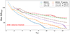 |
Fig. B.1. Evolution of the maximum iS/Nmed with increasing zsim for GRB 090424, GRB 110731A, and GRB 120119A. The shaded area corresponds to the 90% confidence interval for the median. The red horizontal line shows the iS/N threshold of 6.5. |
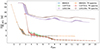 |
Fig. B.2. Similar to Figure 8, but for GRB 090424, GRB 110731A, and GRB 120119A and including also the TR spectral model analysis along with the TI spectral model for comparison. |
In Figure B.1, the iS/Nmed curves for GRB 110731A show minor differences between the two scenarios. For GRB 090424 and GRB 120119A the disparities are more noticeable, though the general patterns remain similar. Above zsim ∼ 2 for GRB 090424 and zsim ∼ 3 for GRB 120119A, the iS/N values slightly favour the TR scenario, leading to a larger zhor value. In the case of GRB 090424 this results in a noticeable difference in the obtained zhor value.
In Figure B.2 the curves for GRB 090424 and GRB 110731A exhibit negligible differences between the two scenarios, and consistent with the derived confidence intervals and the uncertainties obtained from battblocks. The curves corresponding to GRB 120119A exhibit slightly more disparities between the scenarios, generally with lower T90 values in the TI scenario, although the general trends remain consistent.
Although this comparison is limited to only three GRBs and may not fully represent the entire sample, its purpose is to demonstrate that while there might be quantitative impacts on the results, the qualitative conclusions remain valid. We recall that there is a limited availability of TR spectra, and hence the adoption of the TI spectra simplification, assuming their potential caveats.
Appendix C: Potential bias in the analysis
The comparison of the  median values obtained for each GRB in the sample at zmeas within ECLAIRs fcFoV, with the measured values from Swift/BAT (hereafter
  and
and  , respectively), revealed a potential bias in the analysis. Specifically, for certain GRBs
  was found to be significantly larger than
  . These GRBs exhibit a common characteristic in their light curves, characterised by a prolonged period over which the count rate remains nearly at the background noise level after the main peak (i.e. long low-flux tail emission).
Figure C.1 illustrates the ratio  plotted against
  (T100 being the time interval that encompasses 100% of the burst counts). The clear trend observed between these two ratios suggests that the inclusion of the long tail emission in the calculated
  values contributes to the observed differences.
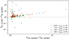 |
Fig. C.1. Comparison between the values of |

A potential explanation for this might be related to the background subtracted light curves from Swift/BAT used as input for the simulations. When the raw light curve exhibits a prolonged time interval with only a few GRB counts above the noise level, the background subtraction procedure may lead to the positive parts of the background noise fluctuations being interpreted as GRB photons, while the negative parts may be subtracted below the estimated background curve. In other words, during the background subtraction, only the positive fluctuations would be retained.
In addition, selecting the time interval and the binning applied to the light curve passed to the battblocks tool may influence the results. In this study, we specifically opted for 80 ms binning and selected the events within 25% before and after the GRB events. This selection might introduce an additional impact on the results, potentially leading to a T90 that is more closely related to the initial  time interval.
However, it is important to note that this bias should not significantly affect the qualitative results concerning the evolution of T90 with redshift, as the input light curve was the same for all zsim values. Additionally, the S/N computation is unlikely to be influenced since the maximum iS/N primarily depends on the intensity of the peak and not on the low-flux tail emission.
Appendix D: Evolution of T90 for each GRB in the sample
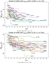 |
Fig. D.1. Analogous to Figure 9 (evolution of |

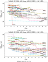 |
Fig. D.1. continued. |
Appendix E: Table of resulting values from the simulations
General results for each GRB in the sample.
All Tables
All Figures
|
Fig. 1. The SVOM mission. (a) Outline of the SVOM mission, including the space and ground instruments. (b) Time and energy coverage of the instruments in the SVOM mission. |
| In the text | |
|
Fig. 2. ECLAIRs flight model: view of the coded mask. |
| In the text | |
|
Fig. 3. Rest-frame T90 as a function of redshift for the GRBs in the sample, colour-coded based on the bursts Eiso. The solid line corresponds to the |
| In the text | |
|
Fig. 4. Flowchart of the simulation structure. The three simulator tools used in the analysis are shown as the blue bricks. This process is parallelised for all simulated GRBs, sky positions, and redshift values. |
| In the text | |
|
Fig. 5. Count-rate evolution of the background measured by ECLAIRs for a standard SVOM orbit, over the 4−120 keV energy range and with a binning of 5.12 s. The contribution of the main background components are displayed in different colours. |
| In the text | |
|
Fig. 6. Mask response as a function of the source direction, for the pixels along the diagonal (green) and horizontal (black) cuts of the FOV. |
| In the text | |
|
Fig. 7. Representation of the positions within the FOV used in each simulation case. The grey-shaded region represents the part of the FoV for which the results of analysis in all the FoV are extrapolated. |
| In the text | |
|
Fig. 8. Evolution of the retrieved 4−120 keV light curves at different zsim for a specific position within the fcFoV, for the three GRBs described as case studies. GRB 140311A, GRB 090424, and GRB 090516A are shown in panels a–c respectively. For better visualisation, different binning is used for each GRB, both axes are fixed for all plots in the same panel, and the y-axis is shown in logarithmic scale in panels b and c. The obtained T90 interval is shown with a grey shaded band on each light curve, and the corresponding values written on top, if the detection was successful. These light curves and values correspond to one trial, and hence they may differ from the values given in the text, which correspond to the median of 100 trials. |
| In the text | |
|
Fig. 9. Evolution of |
| In the text | |
|
Fig. 10. Percentage of detected GRBs within ECLAIRs fcFoV at each simulated redshift for the whole sample, separated into subsets based on their zmeas. The numbers shown at the top of the histogram correspond to the number of detected GRBs in each redshift. |
| In the text | |
|
Fig. 11. Comparison of the iS/Nmed obtained with Elow values of 15 and 4 keV, for all GRBs, and redshift values simulated within the fcFoV. The blue and grey points represent respectively all successful and not successful detections with Elow = 4 keV. The red vertical line represents the iS/N threshold above which the successful detections with Elow = 15 keV lie. |
| In the text | |
|
Fig. 12. Comparison of the percentage of detected GRBs (iS/Nmed ≥ 6.5) within the fcFoV at each zsim for Elow values of 15 and 4 keV. The dashed red line represents the relative difference between the percentage of both scenarios, with respect to the 4 keV scenario. |
| In the text | |
|
Fig. 13. Fraction of the FoV with successful detection (iS/N ≥ 6.5) plotted against zsim for each GRB in the sample (grey curves). The median and mean values for bins of 0.5 width in redshift are shown in blue and orange, respectively. |
| In the text | |
|
Fig. 14. Evolution of |
| In the text | |
|
Fig. B.1. Evolution of the maximum iS/Nmed with increasing zsim for GRB 090424, GRB 110731A, and GRB 120119A. The shaded area corresponds to the 90% confidence interval for the median. The red horizontal line shows the iS/N threshold of 6.5. |
| In the text | |
|
Fig. B.2. Similar to Figure 8, but for GRB 090424, GRB 110731A, and GRB 120119A and including also the TR spectral model analysis along with the TI spectral model for comparison. |
| In the text | |
|
Fig. C.1. Comparison between the values of |
| In the text | |
|
Fig. D.1. Analogous to Figure 9 (evolution of |
| In the text | |
|
Fig. D.1. continued. |
| In the text | |
Current usage metrics show cumulative count of Article Views (full-text article views including HTML views, PDF and ePub downloads, according to the available data) and Abstracts Views on Vision4Press platform.
Data correspond to usage on the plateform after 2015. The current usage metrics is available 48-96 hours after online publication and is updated daily on week days.
Initial download of the metrics may take a while.