| Issue |
A&A
Volume 685, May 2024
|
|
|---|---|---|
| Article Number | A160 | |
| Number of page(s) | 50 | |
| Section | Planets and planetary systems | |
| DOI | https://doi.org/10.1051/0004-6361/202347925 | |
| Published online | 22 May 2024 | |
Modeling the structure of the dayside Venusian ionosphere: Impacts of protonation and Coulomb interaction
1
Planetary Environmental and Astrobiological Research Laboratory (PEARL), School of Atmospheric Sciences, Sun Yat-sen University,
Zhuhai,
Guangdong,
PR China
e-mail: This email address is being protected from spambots. You need JavaScript enabled to view it.
2
Chinese Academy of Sciences Center for Excellence in Comparative Planetology,
Hefei,
Anhui,
PR China
Received:
9
September
2023
Accepted:
23
February
2024
Abstract
Context. The CO2-dominated thick atmosphere of Venus coexists with an ionosphere that is mainly formed, on the dayside, via the ionization of atmospheric neutrals by solar extreme ultraviolet and soft X-ray photons. Despite extensive modeling efforts that have reproduced the electron distribution reasonably well, we note two main shortcomings with respect to prior studies. The effects of pro-tonation and Coulomb interaction are crucial to unveiling the structure and composition of the Venusian ionosphere.
Aims. We evaluate the role of protonated species on the structure of the dayside Venusian ionosphere for the first time. We also evaluate the role of ion-ion Coulomb collisions, which are neglected in many existing models.
Methods. Focusing on the solar minimum condition for which the effect of protonation is expected to be more prominent, we constructed a detailed one-dimensional photochemical model for the dayside Venusian ionosphere, incorporating more than 50 ion and neutral species (of which 17 are protonated species), along with the most thorough chemical network to date. We included both ion-neutral and ion-ion Coulomb collisions. Photoelectron impact processes were implemented with a two-stream kinetic model.
Results. Our model reproduces the observed electron distribution reasonably well. The model indicates that protonation tends to diverge the ionization flow into more channels via a series of proton transfer reactions along the direction of low to high proton affinities for parent neutrals. In addition, the distribution of O2+ is enhanced by protonation by a factor of nearly 2 at high altitudes, where it is efficiently produced via the reaction between O and OH+. We find that Coulomb collisions influence the topside Venusian ionosphere not only directly by suppressing ion diffusion, but also indirectly by modifying ion chemistry. Two ion groups can be distinguished in terms of the effects of Coulomb collisions: one group preferentially produced at high altitudes and accumulated in the topside ionosphere, which is to be compared with another group that is preferentially produced at low altitudes and, instead, depleted in the topside ionosphere.
Conclusions. Both protonation and Coulomb collisions have appreciable impacts on the topside Venusian ionosphere, which account for many of the significant differences in the model ion distribution between this study and early calculations.
Key words: planets and satellites: atmospheres / planets and satellites: composition / planets and satellites: terrestrial planets / planets and satellites: individual: Venus
© The Authors 2024
 Open Access article, published by EDP Sciences, under the terms of the Creative Commons Attribution License (https://creativecommons.org/licenses/by/4.0), which permits unrestricted use, distribution, and reproduction in any medium, provided the original work is properly cited.
This article is published in open access under the Subscribe to Open model. This email address is being protected from spambots. You need JavaScript enabled to view it. to support open access publication.
1 Introduction
Venus contains a thick CO2-dominated atmosphere that is speculated as being wet in the distant past, but dry at present owing to strong atmospheric escape over its evolutionary history (e.g., Gillmann et al. 2022). This scenario is supported by the observation of an exceptionally large deuterium-to-hydrogen ratio in its atmosphere (Donahue et al. 1982; de Bergh et al. 1991; Grinspoon 1993). The upper portion of the Venusian atmosphere also coexists with an ionosphere above the altitude of 100 km (Brace & Kliore 1991; Gérard et al. 2017, and references therein). Its first-ever observation dates back to more than 50 yr ago, when the Mariner 5 spacecraft flew by the planet and made a radio occultation (RO) measurement of the vertical electron distribution (Kliore et al. 1967). This early observation showed that the dayside Venusian ionosphere was characterized by a peak electron density of (5−6) × 105 cm−3 near 140 km (Kliore et al. 1967). The Mariner 5 RO measurements were followed (and confirmed) by similar measurements made on board several later spacecrafts such as Mariner 10 and Venera 9 and 10 (e.g. Fjeldbo et al. 1975; Ivanov-Kholodny et al. 1979). Analogous to most solar system bodies, the ionosphere of Venus on the sunlit side is mainly produced via the ionization of atmospheric neutrals by solar extreme ultraviolet (EUV) and soft X-ray (SXR) photons, along with the impact ionization by concomitant photoelectrons and their secondaries (Witasse et al. 2008).
Over the past few decades, extensive efforts have been devoted to understanding the response of the Venusian ionosphere to a number of controlling factors, in particular, the solar illumination condition, thanks to the large number of electron density profiles accumulated by Pioneer Venus Orbiter (PVO; Kliore et al. 1979), Venus Express (VEx; Pätzold et al. 2007), and (more recently) Akatsuki (Imamura et al. 2011), among others. Existing studies reveal that the main part of the dayside Venusian ionosphere is composed of two distinct layers: a primary V2 layer and a lower secondary V1 layer, produced via the interactions of the atmosphere with different portions of the solar spectrum (Pätzold et al. 2007; Girazian et al. 2015; Tripathi et al. 2023). The majority of the VEx RO measurements also revealed the presence of a third V3 layer at 160–180 km, which has not been satisfactorily explained since it was first reported by Pätzold et al. (2007).
The structures of both layers have been observed to vary systematically with the solar zenith angle (SZA) and incident solar EUV and SXR irradiance, featured by a higher peak electron density at solar maximum than at solar minimum (e.g., Cravens et al. 1981; Kliore & Mullen 1989; Girazian et al. 2015; Tripathi et al. 2023). Kliore & Mullen (1989) combined the PVO and Venera RO data to obtain a power-law dependence of the V2 peak density on the incident solar EUV flux, characterized by a power index of 0.376. Girazian et al. (2015) used the VEx RO data to find that the SZA variations of the peak electron density and altitude were compatible with the prediction of the idealized Chapman theory, at different solar activities and for both the V2 and V1 layers. Similar variations were also reported above the V2 peak, manifest as a more pronounced response of the topside electron density to solar irradiance at higher altitudes (Hensley et al. 2020). As for the peak electron altitude, Cravens et al. (1981)’s analysis of the early Mariner and Venera RO data suggested that the V2 peak altitude remained roughly constant from subsolar to SZA ~ 60°, declined modestly by 5 km to SZA ~ 80°, and then increased abruptly by at least 10 km near the terminator. These authors further proposed that extra controlling factors should be invoked to account for the full observed ionospheric variability on Venus, such as the cooling of the dayside upper atmosphere at large SZA.
In addition to the electron distribution, information on the ion composition is available owing to the extensive in situ measurements made by the PVO ion mass spectrometer, including  , and He+ (Taylor et al. 1979b,a, 1980). Unlike the RO measurements which were carried out through the entire PVO mission, in situ density measurements of individual ion species have been restricted to a much shorter time span of 19 months when the spacecraft periapsis was lowered to the vicinity of 150 km in altitude, covering moderately high to high solar activity conditions (Brace & Kliore 1991). Analysis of these measurements indicates that
  is the most abundant ion species at low altitudes (encompassing the V2 and V1 peaks) despite the dominance of CO2 in the ambient atmosphere, whereas O+ becomes more abundant well above the V2 peak (Taylor et al. 1980).
The available information on the Venusian ionospheric composition motivates continuous modeling studies over the past few decades, from simple ones that either assume photochemical equilibrium (PCE) or include a limited number of ion species (e.g., McElroy 1968; Herman et al. 1971; Chen & Nagy 1978; Nagy et al. 1980; Taylor et al. 1980; Cravens et al. 1981; Peter et al. 2014; Ambili et al. 2019) to more sophisticated ones that take into account both photochemistry and ion diffusion, and simultaneously include a substantially larger list of ion species (e.g., Fox & Sung 2001; Fox & Paxton 2005; Fox 2007b, 2008). The construction of these models not only helps to deepen our understandings of the Venusian ionospheric structure and make predictions for the dayside ion composition at solar minimum for which no available measurements exist, but it also allows many important processes in the coupled Venusian upper atmosphere and ionosphere to be explored in detail, including: neutral heating (Fox 1988), airglow emission (Fox & Bougher 1991; Gérard et al. 2017), and atmospheric escape (Donahue & Hartle 1992; Krasnopolsky & Gladstone 2005; Gu et al. 2021).
Without atomic O in the background atmosphere, early models such as those of McElroy (1968) and Herman et al. (1971) incorrectly concluded that the dayside Venusian ionosphere was dominated by  . Later models by Kumar & Hunten (1974) and Nagy et al. (1975) showed that, by incorporating a small amount of O (1% at the homopause),
  could be rapidly converted to
  via
via

making  significantly more abundant than
  at all altitudes. Both models did not take into account the known effect of photoelectron impact ionization. This process was first considered by Chen & Nagy (1978) based on a two-stream kinetic approach and also by most of the subsequent modelers using a variety of techniques.
More recent models have taken into account a more complicated species list and photochemical network appropriate for the dayside Venusian ionosphere. The model from Fox & Sung (2001) serves as a benchmark, incorporating a total number of 13 ions and 7 extra minor neutrals, embedded within a background atmosphere composed of 10 neutrals. Fox & Sung (2001), along with several subsequent studies by the same leading author (Fox & Paxton 2005; Fox 2007b, 2008), considered both ground-and excited-state species, included the effects of molecular and eddy diffusion, and constructed the background atmosphere based on the widely used global empirical model of the Venusian thermosphere published by Hedin et al. (1983), usually referred to as the VTS3 model. It is also noteworthy that a recent model developed by Peter et al. (2014), being PCE in nature, used the Venus Global Reference Atmosphere Model (VenusGRAM) for the background atmosphere (Kliore et al. 1985), but VenusGRAM was later suggested to be less realistic than VTS3 (Ambili et al. 2019).
Despite the availability of the PVO mass spectrometer measurements for individual ion species, most existing calculations for the Venusian ionospheric structure and composition have been validated by comparing to the RO-based electron distribution in terms of the peak density and altitude only (e.g., Fox 2007b; Peter et al. 2014; Ambili et al. 2019). Broad data-model agreement has been achieved by these models. For instance, Fox (2007b) reproduced fairly well the location of the V2 peak, despite that the V2 peak density was underestimated slightly by 20%–40%. A few studies focused on the topside electron distribution (Nagy et al. 1975; Fox 2007b), all indicating that without invoking a substantial upward ion flux, the topside electron density would be seriously overestimated. Fox (2007b) used the measured ratio of the electron density at 300 km to the V2 peak density to infer an average upward ion flux of ~ 2 × 108 cm−2 s−1.
Since the most chemically robust models up to now were developed more than 20 yr ago, it is timely to reinvestigate the structure and composition of the Venusian ionosphere, especially in view of our greatly improved understandings of ionospheric chemistry over the past few years, partly owing to similar modeling studies of the Martian ionosphere (e.g., Fox et al. 2015; Fox 2015; Lo et al. 2020; Wu et al. 2021). In particular, all existing models of the Venusian ionosphere have not taken into account the protonated species, which may have appreciable concentrations based on our experience with Mars (Fox et al. 2015; Fox 2015). The protonated species can be favorably produced and destructed by proton transfer and other reactions, in the presence of even a small amount of hydrogen in the background atmosphere. This is indeed the case for both Mars and Venus.
For Mars, protonated species have been observed to be common in the dayside ionosphere, some of which have fairly large concentrations (e.g., Benna et al. 2015) and are known to drive strong hydrogen escape during both quiet times and global dust storms (e.g., Krasnopolsky 2019; Stone et al. 2020). For Venus, despite the lack of direct observations, the simultaneous in situ measurements of H+, O+, O, and CO2 in the coupled upper atmosphere and ionosphere implies a large atomic H concentration of 5 × 104 cm−3 on the dayside; whereas the nightside concentration could be even higher by two orders of magnitude (Brinton et al. 1980; Taylor et al. 1984). As shown by our model, the inferred atmospheric hydrogen distribution on Venus is sufficient to cause substantial protonation. The neglect of this process is clearly a common drawback in all existing models of the Venusian ionosphere.
A second (and equally important) drawback is that most of the previous model studies either ignored diffusion at all (i.e., PCE in nature) or ignored the Coulomb interaction when characterizing ion diffusion within the background atmosphere. Again, our experience with Mars suggests that whether or not the Coulomb interaction is taken into account may have significant consequences on the model results (Matta et al. 2013). The recent investigation of Cao et al. (2023) demonstrates that, at 160 km or higher in the Martian upper atmosphere, which is below the normal PCE boundary (Mendillo et al. 2011), the Coulomb interaction prevails over the ion-neutral interaction in controlling ion diffusion.
The above considerations motivate us to construct an updated model of the dayside Venusian ionosphere by including both protonation and Coulomb interaction. As detailed in the paper, the new model would particularly improve our understandings of the properties of the topside ionosphere, where protonation becomes important due to the diffusive separation of atmospheric hydrogen; in addition, Coulomb interaction also becomes important due to the relatively large scale height of ionospheric plasma. The layout of the paper is as follows. In Sect. 2, we describe the model details, such as the structure of the background atmosphere and the incident solar EUV and SXR spectrum. In Sect. 3, we present the model results, which are compared to those of Fox & Sung (2001, hereafter denoted as FS01) and validated with existing RO measurements of the electron distribution. The impacts of protonation and Coulomb interaction on the Venusian ionosphere are elaborated in Sect. 4, followed by a thorough discussion of the model discrepancies between this study and FS01 in Sect. 5. Finally, we summarize and draw conclusions in Sect. 6. A substantial amount of supplementary information is provided in the appendices for reference, including the details of the diffusion coefficients, cross-sections, and chemical rate constants, as well as a thorough description of the dominant chemical production and destruction pathways for each species included in our model.
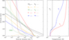 |
Fig. 1 Structure of the underlying Venusian upper atmosphere used in our model calculations, appropriate for the dayside averaged condition at solar minimum. Left: density profiles of 10 background species (CO2, O, CO, N2, N, He, O2, H2, H, and Ar). For comparison, we also show the H2 density profile adopted by FS01 for solar minimum, which presents the most pronounced distinction from our choice among all species. Right: neutral, ion, and electron temperature profiles (denoted as Tn, Ti, and Te, respectively). |
2 Model description
2.1 General remarks
Our background atmosphere contains ten species: CO2, O, CO, N2, N, He, O2, H2, H, and Ar. Their density profiles are depicted in Fig. 1 (left) over the altitude range of 100–350 km. The density profiles of the first six species, along with the respective neutral temperature profile, as shown in Fig. 1 (right), were constructed on basis of the VTS3 model of Hedin et al. (1983). The VTS3 model was established with the aid of the PVO neutral mass spectrometer (Niemann et al. 1980) and atmospheric drag (Keating et al. 1980) measurements. A fixed SZA of 60° was used throughout this study. The density profiles of the remaining background species were modeled with the conventional diffusion equation, including the effects of molecular, eddy, and thermal diffusion. The thermal diffusion coefficient was set as −0.25 for H and H2, and 0 for the others. The choice of the molecular diffusion coefficient for each binary gas mixture is described in Appendix A. The eddy diffusion coefficient was parameterized exactly the same as in FS01, reflecting atmospheric mixing due to both large scale winds and small scale turbulences. To construct the density profiles of O2, H2, H, and Ar with the diffusion equation, we used the same boundary conditions for the latter three as in FS01. For O2, a more recent mixing ratio of 300 ppm was adopted at the bottom boundary (Fox & Paxton 2005), as constrained by the atomic C abundance inferred from the PVO ultraviolet spectrometer limb observations of two resonance lines at 1561 Å and 1657 Å. The ion and electron temperature profiles appropriate for our solar minimum calculations are also adopted from FS01, as displayed in Fig. 1 (right).
The structure of our background atmosphere is nearly identical to that of FS01, except for a few noticeable distinctions. The different choice of the O2 mixing ratio at the bottom boundary, as mentioned above, leads to a large difference in the O2 distribution between the two studies by an order of magnitude at all altitudes. However, the most important difference occurs for the distribution of H2, as shown in Fig. 1 (left), which is mainly driven by different molecular diffusion coefficients used by different authors. In particular, our imposed molecular diffusion coefficient is substantially higher than that of FS01, implying a lower homopause altitude for H2 in the background atmosphere. More details on this issue are provided in Appendix A.
The background atmosphere and incident solar spectrum (described below in Sect. 2.2) are used as model inputs to characterize the structure and composition of the sunlit Venusian ionosphere on average, incorporating the effects of both photochemistry and ion diffusion. A total number of 30 ion species are included:  , and HOCO+ in the order of increasing mass. Here, O+(4S) refers to the ground state of O+, whereas O+(2D) and O+(2P) refer to the excited states. The ion species list that we choose is considerably more thorough than that of FS01. In particular, the presence of hydrogen in atomic or molecular form in the background atmosphere (see Fig. 1, left) is expected to trigger the formation of a bunch of protonated species (Fox et al. 2015; Fox 2015), which we explore here for the first time for Venus. In fact, more than half of the ion species included in our calculations are protonated species. For ion diffusion, the effects of both ion-neutral and ion-ion Coulomb collisions are incorporated (see Appendix A for details).
Furthermore, 11 extra neutral species, including C, C(1D), C(1S), N(2D), N(2P), O(1D), O(1S), CH, NH, OH, and NO are treated as unknowns, whose density profiles are not imposed a priori but solved self-consistently by the model. C(1D), C(1S), N(2D), N(2P), O(1D), and O(1S) refer to excited-state species, to be distinguished from their ground-state counterparts abbreviated as C, N, and O, respectively. For neutrals, their ground-state abundances are typically much higher than the abundances of the same species at the excited states. Hence, we use the atomic symbol without specified electronic state to represent either the ground state or the sum of all states. This is not the case for O+ as the abundance of excited-state O+ (2D) is not too much lower than that of ground-state O+(4S) (see Sect. 3 for details). Accordingly, all electronic states of O+ are explicitly specified throughout the paper.
In this study, we implemented a photochemical network that is more complex than those used previously. For easy reference, we provide detailed information on the photon impact processes, photoelectron impact processes, as well as chemical reactions incorporated in our model in Appendices B and C, respectively.
In particular, we adopted a comprehensive chemical network that includes 363 ion-neutral reaction channels (see Table C.1), 54 recombination channels (8 radiative recombination channels and 46 DR channels, see Table C.2), 105 neutral-neutral reaction channels (see Table C.3), and 63 deexcitation channels (11 channels via spontaneous emission, 11 channels via collisional quenching by electrons, and 41 channels via collisional quenching by neutrals, see Tables C.4 and C.5). Three-body reactions are neglected in the model. A total number of 49 photon impact processes are included in our chemical scheme: 17 photodissociation channels and 32 photoionization channels (see Table B.1). Meanwhile, we take into account a large number of 463 photoelectron impact processes: 12 elastic collision channels, 44 vibrational excitation channels, 377 electronic excitation channels, and 30 ionization channels (see Table B.2). We caution that elastic collisions and vibrational and electronic excitations do not directly affect the ionospheric chemistry (except for the production of excited-state neutrals in our species list via photoelectron impact), but these processes are critical for an accurate modeling of photoelectron energy degradation (see Sect. 2.3) and thereby exert an indirect influence on ion production by photoelectron impact.
The model is implemented by solving simultaneously the density and velocity profiles of all unknown species based on the coupled continuity and momentum equations. Solving the energy equation is not required as the temperature profiles are fixed as model inputs. For all species, we assume PCE at the lower boundary and diffusive equilibrium at the upper boundary. The equations are solved from “zero” plasma content by imposing a constant time step of 0.03 s. We use the splitting method to deal with the continuity and diffusion equations separately. At each time step, the chemical solver uses the exponential differencing expression of Mendillo et al. (2011, see their Eq. (1)) which avoids density overshoot and allows faster convergence than the traditional explicit or implicit method (Martinis et al. 2003), whereas the diffusion solver uses the Crank-Nicholson method to solve the associated tridiagonal matrix by Gaussian elimination (Johnstone et al. 2018, see their Appendix E). For each species, its density and velocity profiles are tracked until the steady-state condition is obtained, defined as when the rate of fractional change in density falls below 10−5 s−1. The whole computational domain is divided into 46 grids with a logarithmically varying resolution from 2.8 km at the bottom to 10 km at the top.
2.2 Solar activity consideration
For the purposes of this study, we focus specifically on the solar minimum condition. In practice, the production of protonated species relies critically on the amounts of H and H2 in the background atmosphere. While the solar cycle variation of the H2 distribution has not been well established, the H distribution was proposed to be significantly reduced at high solar activity, as the outcome of enhanced H escape via charge exchange and ambipolar electric field acceleration (e.g., Hartle et al. 1996). As a consequence, we speculate that the effect of protonation on the Venusian ionosphere is suppressed at high solar activity. This is indeed the case as our test model runs with different incident solar spectra (and the appropriate background atmospheres from the VTS3 model) reveal that the total concentrations of protonated species are reduced at solar maximum, despite the fact that the total ionospheric plasma concentration is enhanced (e.g., Cravens et al. 1981; Kliore & Mullen 1989; Girazian et al. 2015; Hensley et al. 2020).
Throughout this study, the incident solar irradiance is based on the Flare Irradiance Spectral Model (FISM) version 2 solar spectrum at the Earth over the wavelength range of 0.05–189.95 nm with a resolution of 0.1 nm (Chamberlin et al. 2020)1. Such a high resolution is necessary for accurately computing the photoionization and photodissociation rates in a planetary upper atmosphere (e.g., Lavvas et al. 2011). Specifically, we used the model spectrum on 25 Jan. 2007 during solar cycle 23, with a 10.7 cm solar radio index of 80 in solar flux units (SFU, i.e., 10−22 W m−2 Hz−1). Such a spectrum is scaled to a mean heliocentric distance of 0.72 astronomical unit for Venus, displayed in Fig. 2 for reference.
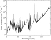 |
Fig. 2 Solar EUV and SXR spectrum (at the top of the Venusian atmosphere) used in our solar minimum model calculations over the wavelength range of 0.05–189.95 nm with a resolution of 0.1 nm. |
2.3 Treatment of secondary ionization
To characterize secondary ionization, we adopted a two-stream kinetic approach that computes the differential electron fluxes in both the upward and downward directions. The energy range that we choose is from 1 eV to 5 keV, divided into 106 logarithmically distributed grids. As quoted above, a large number of photoelectron-neutral collision channels (elastic, vibrational/electronic excitation, and ionization) are incorporated in the model. The Coulomb interaction between photoelectrons and main ionospheric electrons is neglected because it only affects the low energy portion of the model photoelectron energy distribution (typically below 10 eV), which is insufficient to trigger collisional ionization; thus, it does not contribute to ionospheric chemistry.
Since photoelectron collision occurs extremely fast, we directly solve the steady-state photoelectron transport equation. In the upward direction, sink terms include the backward scattering of upward propagating photoelectrons via elastic collisions and the energy degradation of upward propagating photoelectrons to lower energy levels via inelastic collisions (both forward and backward), whereas source terms include the backward scattering of downward propagating photoelectrons via elastic collisions, the forward and backward scattering of upward and downward propagating photoelectrons via energy degradation from higher energy levels, as well as the production of upward propagating photoelectrons via photoionization. Similar source and sink terms are considered for photoelectrons moving in the downward direction.
The Crank-Nicholson method is used for obtaining numerical solutions for the differential photoelectron flux as a function of both the altitude and energy. The lower boundary condition is chosen to be local energy degradation in both directions. At the upper boundary, a zero downward flux (implying no external electron precipitation) and constant upward flux gradient are assumed. For reference, we show in Fig. 3 the photoelectron energy spectra in the two directions and at two representative altitudes. Notable photoelectron signatures such as the He II peak and aluminum edge are clearly visible (Coates et al. 2008; Tsang et al. 2015). The photoelectron energy spectra in the two opposite directions are comparable at low altitudes as a consequence of near local energy degradation. With increasing altitude, however, the upward flux may greatly exceed the downward flux. Existing model calculations indicate that the high-altitude photoelectrons are not created locally but instead transported from their low-altitude source regions (Cui et al. 2011).
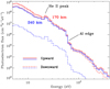 |
Fig. 3 Photoelectron energy spectra in the upward (solid) and downward (dashed) directions in the dayside Venusian ionosphere, at two representative altitudes as indicated in the figure legend. Notable photoelectron signatures, such as the He II peak and aluminum edge, are clearly visible. |
3 Model results
With the model setup described above, we compute numerically the steady-state density profiles of various ions (along with the extra minor neutrals) in the coupled Venusian upper atmosphere and ionosphere appropriate for the dayside averaged condition at solar minimum. We show in Fig. 4 (left) the ion production rate profiles via photoionization (solid) and photoelectron impact ionization (dashed) for several selected species, denoted as primary and secondary ionization, respectively. Primary ionization surpasses secondary ionization at most altitudes near and above the peak, except for the low-altitude regions, where more energetic photons tend to penetrate and create more photoelectrons with sufficient energy to cause (multiple) impact ionization.
The ionization efficiency for each species is further displayed in Fig. 4 (right) as a function of the altitude, defined as the ratio of the secondary to primary ion production rate (Richards & Torr 1988). As expected, the ionization efficiency is always much less than unity at high altitudes, but increases with decreasing altitude. Above 250 km, the ionization efficiency is near constant: 3.4% for  , 6.8% for O+(4S), 2.6% for O+(2D), 2.0% for O+(2P), 3.1% for CO+ and 4.5% for
  At the bottom boundary, the ionization efficiency reaches as large as 8.4 for
  6.2 for O+(4S), 18 for O+(2D) and O+(2P), 6.5 for CO+ and 29 for
  . Our calculations suggest an identical contribution from primary and secondary ion production at 132 km for
  , slightly lower near 130 km for O+(4S), O+(2D), O+(2P), and CO+, and slightly higher at 134 km for
  .
.
The model ion density profiles are shown in Fig. 5, revealing the presence of a visible layer structure for each species, well known to be formed due to the combined effect of increasing density and decreasing solar irradiance, both with decreasing altitude (Fox et al. 2008). Secondary peaks are also visible for most species, though typically manifest as shoulders below the main peaks. The presence of secondary peaks is driven by the penetration of energetic photons (such as in the SXR band) into the deep atmosphere.
Ion density measurements in the dayside Venusian ionosphere are only available from the PVO Ion Mass Spectrometer measurements when the spacecraft periapsis descended to as low as 150 km (Taylor et al. 1979b,a, 1980), but this occurred nearly exclusively at solar maximum. Therefore in this study, we make data-model comparison in terms of the electron distribution only, as depicted in Fig. 6, with the aid of the VEx (Pätzold et al. 2007) and Akatsuki (Imamura et al. 2011) RO measurements. The solid circles in the figure show our nominal model profile appropriate for the dayside averaged condition at solar minimum. The red symbols represent three electron density profiles obtained by the MEx RO experiments performed in July 2006, all appropriate for the solar minimum condition and with a similar SZA of 50°–60°, whereas the blue symbols represent another set of three electron density profiles obtained by the Akatsuki RO experiments performed over a much longer period with the 10.7 cm solar radio index ranging from 67 to 112.4 SFU and SZA from near subsolar to near terminator. The MEx and Akatsuki profiles were based on the results published in Pätzold et al. (2007) and Tripathi et al. (2023), respectively. For further comparison, we also show with the green symbols in the same figure, three extra electron density profiles based on the empirical model of Theis et al. (1984) appropriate for three different SZA values but all for the solar maximum condition.
Our model electron density distribution is broadly consistent with the available RO measurements at solar minimum, up to at least 250 km. The PVO-based electron densities for the same SZA are higher than ours as expected because the PVO measurements were obtained at higher solar activity. Two out of the three Akatsuki electron density profiles show peak densities higher than our model peak density by 50%, because one of them probes a similar solar activity but lower SZA while the other one probes a similar SZA but a higher solar activity. Compared with the remaining RO profiles obtained at similar solar illumination conditions, we may infer from Fig. 6 that the observed peak electron density is slightly higher than the model value by 20%, which could be due to a variety of reasons such as the uncertainties in the incident solar spectrum, the background atmosphere, the photon impact or photoelectron impact cross-sections, as well as the recombination rate coefficients.
The data-model comparison at high altitudes deserves some more concern. On the one hand, the RO measurements at solar minimum tend to be slightly lower than our prediction in the topside ionosphere, by as much as 30% near 200 km. On the other hand, the RO measurements at even higher altitudes render significant variation in electron distribution which does not follow regularly the variation of the solar illumination condition. These two features imply that some extra processes might be in function but are not incorporated in the model. One possibility is the presence of strong ionospheric plasma outflow on Venus, as suggested by Fox (2008) for the solar maximum condition. This author predicted an average dayside O+ escape flux of ~2 × 108 cm−2 s−1, which was thought to be mainly associated with the cross-terminator plasma flow and thus responsible for maintaining a nightside ionosphere on Venus (Knudsen et al. 1980; Spenner et al. 1981; Knudsen & Miller 1992). Another possibility is related to the interaction of the Venusian ionosphere with the upstream solar wind (Luhmann 1986; Futaana et al. 2017, and references therein). The electron density in the Venusian ionosphere drops rapidly on the sunlit side near the altitude where the external solar wind dynamic pressure is balanced by the internal ionospheric thermal pressure (Phillips et al. 1985, 1988; Han et al. 2020), as clearly seen in several RO profiles displayed in Fig. 6. Based on the early PVO measurements, Mahajan & Mayr (1989) reported that for the solar minimum condition, the topside Venusian ionosphere was strongly disturbed by the solar wind induced plasma transport, manifest as a scale height substantially smaller than that expected for the undisturbed diffusive equilibrium condition (see also Mahajan et al. 1989). Both effects outlined above may contribute to the data-model discrepancy at high altitudes as witnessed in Fig. 6. A more robust characterization of the topside Venusian ionosphere, especially when the solar wind dynamic pressure becomes high, is beyond the scope of this study and must rely on three-dimensional magnetohydrodynamic simulations that incorporate solar wind interactions (e.g., Terada et al. 2009; Ma et al. 2013; Lu et al. 2015; Dang et al. 2023).
We now focus on individual ion species common to both this study and FS01. A comparison of selected ion density profiles is shown in Fig. 7, highlighting those with significant discrepancies between the two studies. The figure illustrates that both studies predict a quite similar electron density profile except near the bottom boundary where the FS01 profile extends further to the low-altitude regions compared with ours. Such a low altitude discrepancy is primarily linked to the model NO+ distribution: FS01 predicts a broader double layer structure, whereas ours predicts a sharper single layer structure.
Well above the V2 peak, the model differences for individual ion species could be fairly large and diverse in spite of the good agreement in electron density (differing by 15% at maximum). Compared with FS01, our model predicts a substantially higher abundance for  in the topside ionosphere above 200 km. Discrepancies also exist for the other species at high altitudes. For instance, an enhanced topside distribution is obtained by our model for relatively light species such as H+ and C+. The discrepancy for C+ is especially large, with our model density higher than the FS01 density by a factor of 6.5 near 300 km. However, such a feature is not common to all species and for some of the displayed ones such as O+(4S) and N+, our predicted topside abundances are substantially lower than the FS01 results.
We further show in Fig. 8 the density profiles of those minor neutral species treated as unknowns in the model. All these species, which are produced via photochemistry, display well-defined layer structures as the ion species. The exact peak density and altitude of each species vary, depending on the detailed chemical production and destruction channels involved, and sometimes rendering multiple layers within the simulation regime such as O(1S) and NO. Similarly to the process described above, we compare in Fig. 8 (left) the minor neutral density profiles for several species obtained by our model with the low solar activity results of FS01. The figure indicates that the two studies generally predict similar density profiles, with two prominent exceptions: one for C with our model peak density higher than the FS01 result by a factor of 2.5 and the other one for NO with our model peak density lower by a large factor of 6.5. It is also noteworthy that the model C peak altitude is comparable between the two studies, but the difference in the NO peak altitude is relatively large, with the FS01 peak altitude located below our bottom boundary. Possible interpretations for the model discrepancies for minor neutrals, along with those for ions reported above, are provided in Sect. 5.
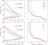 |
Fig. 4 Comparison of ion production rate and ionization efficiency for several selected species. Left: ion production rate profiles associated with primary (solid) and secondary (dashed) ionization. Right: respective ionization efficiency profiles. Primary ionization refers to photoionization and secondary ionization refers to photoelectron impact ionization, respectively. The ionization efficiency is defined as the ratio of the secondary to primary ion production rate. |
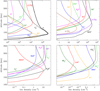 |
Fig. 5 Dayside averaged density profiles of various ion species in the Venusian ionosphere based on our solar minimum model calculations. All species display well-defined peak structures, usually superimposed by secondary peaks at lower altitudes though typically manifest as shoulders. The thick solid line in the upper left panel represents the electron distribution inferred from charge neutrality. |
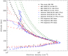 |
Fig. 6 Comparison of the electron density distribution between this study (appropriate for a SZA of 60° and a 10.7 cm solar radio index of 80 SFU) and various measurements. The solid circles are for the model density profile, the red symbols are for the VEx RO measurements covering a narrow SZA interval of 50°–60° and all at solar minimum, the blue symbols are for the Akatsuki RO measurements covering wider ranges of both SZA and 10.7 cm solar radio index, whereas the green symbols are extracted from the empirical model of Theis et al. (1984) based on the PVO in-situ measurements at solar maximum. Numbers starting with “S” and “F” refer to the corresponding values of the SZA (in degree) and 10.7 cm solar radio index (in SFU). “Smax” stands for “solar maximum.” The dates when the MEx and Akatsuki RO experiments were made are indicated in the figure legend for reference. |
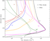 |
Fig. 7 Comparison of the ion density profiles at solar minimum between this study (solid) and FS01 (dashed). |
4 Impacts of Coulomb collisions and protonation
In Appendix D, we present a detailed description of the chemical scheme for each species (both ions and minor neutrals) involved in our calculations. The dominant production or destruction channel is critically controlled by the abundance of the neutral reactant in the background atmosphere, hence varying considerably with the altitude due to diffusive separation (see Fig. 1 left). Typically, the dominant destruction channel for a nonterminal ion species is its reaction with CO2 at low altitudes. With increasing altitude, its reaction with O becomes progressively more important until surpassed by its reaction with H2 typically operating at very high altitudes only. The above general trend, provided that all reactions are energetically allowed, is evidently driven by the differentiation of different neutral reactants according to their masses.
Excited-state chemistry has an important influence on the coupled Venusian upper atmosphere and ionosphere. Several aspects of such an influence are summarized here for easy reference. Firstly, O+(2D) is relatively abundant and enhances the production of many ion species including  , and
, and  at high altitudes via charge exchange between O+(2D) and the respective parent neutrals:

Excited-state O+(2D) is necessary for these production channels to be viable because analogous reactions involving ground-state O+(4S) are all endothermic and hence not allowed at typical ionospheric temperatures. Secondly, excited-state N(2D) critically controls the production (and hence the abundance) of NO via the reaction:

Thirdly, excited-state atoms are crucial for producing the bulk of the CH, NH, and OH radicals in the Venusian upper atmosphere, via the reactions of H2 with C(1D), N(2D), and O(1D):

In general, we may conclude that without excited-state chemistry, the abundances of many ion species and minor neutral species would be significantly under-predicted.
Section 3 presents exhaustive comparisons among our model results and the early FS01 results. Both models predict essentially the same prevailing production and destruction pathways for common species included in the calculations, though exceptions do occur (see Sect. 5 for details). When summed over all ions, our model predicts an electron distribution in good agreement with that of FS01 (and also with existing RO measurements at similar solar illumination conditions). However, the agreement in the distributions of individual ions or minor neutrals between the two models is clearly species-dependent, with some being satisfactory and some others showing considerable discrepancies. Certain discrepancies are common to a range of species, which we attribute to the effects of either Coulomb interaction or protonation, as explained below.
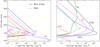 |
Fig. 8 Dayside averaged density profiles of various minor neutral species based on our solar minimum model calculations, all displaying well-defined layer structures. A comparison for some species between this study (solid) and FS01 (dashed) is also indicated in the left panel. |
4.1 Coulomb interaction
One important distinction between this study and FS01 is that our model includes the effects of both ion-neutral and ion-ion Coulomb collisions, while the early study did not consider the latter. Coulomb collisions are known to influence significantly the structure of the topside Martian ionosphere as modeled by Matta et al. (2013) and we expect a similar influence to occur on Venus. A comparison of the total ion (or electron) distribution between the two model runs is demonstrated in Fig. 9, with the solid line showing our nominal model profile with both ion-neutral and ion-ion diffusion included, and the dashed line showing the model profile obtained by including ionneutral diffusion only as in FS01. A non-negligible distinction between the two model ionospheres is evident, especially at high altitudes where diffusion dominates over photochemistry. In general, the total ion distribution is enhanced when both collisions are included, because ion diffusion tends to be slowed down in the topside ionosphere due to increased collision frequency (Matta et al. 2013). However, a careful examination reveals some more complicated effects.
First, our model reveals that not all ion species are enhanced in the topside ionosphere when Coulomb collisions come into effect. The net effect of momentum transfer via Coulomb collisions should be zero, implying that some ions are subjected to upward forces whereas the others subjected to downward forces.
This can be clearly seen in Fig. 9 where we compare the summed density profiles of two ion groups: group I including all species with peak altitudes above 200 km (H+,  ,
,  , He+, HeH+, C+, CH+,
  , N+, NH+,
  , N2H+, O+(4S), O+(2D), OH+, H2O+, H3O+, HOC+, HNO+, ArH+, see Fig. 5) and group II including the remaining species. According to the figure, Coulomb collisions tend to redistribute different ion species in such a way that the group II ions are depleted in the topside ionosphere whereas the group I ions are accumulated instead. This is not a mass-dependent effect because for any species, the gravity force is the same for different model runs. Rather it is an effect closely linked to diffusion. For the group II ions, they are preferentially produced at low altitudes and would diffuse upward as driven by the pressure gradient force. When diffusion is suppressed by including Coulomb collisions, upward diffusion would become more difficult and as a consequence, the group II ions tend to reside deeper in the atmosphere as seen in Fig. 9. A similar line of reasoning accounts for the difference in the group I ion distribution between the two model runs.
Secondly, a detailed inspection of the model results reveals that Coulomb collisions exert different impacts both on the distribution of different species and on the distribution of a single species at different altitudes. This is evidently because the dominant production and destruction mechanisms for individual ion species are diverse as discussed extensively in Appendix D.1. With the redistribution of a given species by Coulomb collisions, the ambient density of the reactant may vary considerably, leading to either enhanced or reduced ion production or destruction rate. In general, the redistribution of a given species must be closely linked to the redistribution of many others through the complicated interweaving photochemical network imposed in our model. Interestingly, for some of the minor neutrals such as excited-state O(1D) and O(1S), our calculations also suggest that their model density profiles at high altitudes are strongly affected by Coulomb collisions. In view of the coupled nature of the Venusian upper atmosphere and ionosphere, this is obviously linked to the modification of photochemistry by ion diffusion.
Finally, we may intuitively expect that the total ion content within the simulation regime is identical between the two model runs, because it is controlled by photochemistry and does not rely on how it is redistributed by diffusion. This is particularly the case for our model calculations assuming PCE at the bottom boundary and diffusive equilibrium at the top boundary (see Sect. 2.1), implying that photochemically produced ions flow neither inside nor outside of the simulation box. However, Fig. 9 shows undoubtedly that the total ion density derived from the nominal model with Coulomb collisions is enhanced at all altitudes, increasing progressively from negligible enhancement at the bottom to an enhancement of nearly 20% at the top. Therefore by including Coulomb collisions, the model simply appears to create more ions, which is counter-intuitive. Such a “dilemma” could be resolved by the following argument. When considering the ionospheric plasma as a whole, it reflects a balance between production via photoionization (along with photoelectron impact ionization) and recombination (DR for molecular ions and radiative recombination for atomic ions). Whether Coulomb collisions are included or not indeed does not affect net production, but it does affect net destruction because when both collisions are operative, photochemically produced ions less easily diffuse away (downward) from their high-altitude source regions (mainly associated with the group I ions) and hence tend to feel a higher environmental electron temperature. This further implies that the high-altitude ions are destructed more slowly in response to the well-known anti-correlation between the electron temperature and the recombination rate, which naturally causes an enhanced total ion content within the simulation regime as witnessed in Fig. 9. Here the redistribution of the group II ions plays a minor role because they preferentially reside at low altitudes where the effect of diffusion is less important.
The discussion above reveals a far more complicated impact on the topside ionosphere exerted by Coulomb collisions than discussed in Matta et al. (2013), not only directly by suppressing ion diffusion, but also indirectly by modifying ion chemistry. To complete this section, we compare in Fig. 10 various time constants estimated in the dayside Venusian ionosphere: ion diffusion time constant (including both ion-neutral and ion-ion diffusion), chemical destruction time constant, as well as ion-neutral and ion-ion collision time constants for several species.
The diffusion time constant near monotonically declines with increasing altitude, whereas the chemical time constant increases instead (except for terminal ions such as  and NO+ below the V2 peak). The PCE boundary, defined as the location where the diffusion and chemical time constants are identical, varies from species to species. For short-lived ions such as
  , the PCE boundary is near 250 km, whereas for long-lived ions such as O+(4S) and
  , the boundary is substantially lower at 185–200 km. It is also clear from Fig. 10 (right) that within the diffusion-dominated regions of the Venusian ionosphere, Coulomb collisions are usually more important than ion-neutral collisions. The ion collision boundary, which we define as the location where the two collision time constants are equal (Cao et al. 2023), is at 140–150 km for all species except for
  , which has a higher boundary near 170 km. Fig. 10 highlights that the Coulomb interaction must be taken into account for a proper characterization of the dayside Venusian ionosphere.
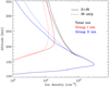 |
Fig. 9 Comparison between two solar minimum model runs, one with ion-neutral (IN) collisions only (dashed) and the other one with both ion-neutral and ion-ion (II) Coulomb collisions (solid). The black lines show the total ion density profiles obtained by the two model runs, whereas the red and blue lines correspond to the density profiles of the group I and II ions, respectively. The former includes all ion species with peak altitudes above 200 km and the latter includes the remaining species. |
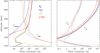 |
Fig. 10 Comparison of various time constants. Left: comparison of the ion diffusion time constant (τdiff) and ion chemical destruction time constant (τchem) for several selected species, where τdiff includes the contributions from both ion-neutral collisions and ion-ion Coulomb collisions. Right: comparison of the ion-neutral collision time constant (τin) and ion-ion Coulomb collision time constant (τii) for the same species. All time constants are based on our solar minimum calculations appropriate for the dayside averaged condition. |
4.2 Protonation
Another important distinction from the early FS01 model is the inclusion of a variety of protonated species in our calculations. These species can be photochemically produced even if a small amount of hydrogen is available in the background atmosphere. In particular, protonation is found to be important for a proper interpretation of the mass spectrometer measurements of the Martian ionosphere (Benna et al. 2015). General remarks on the chemistry of protonated species have been nicely provided in Fox (2015).
On planetary bodies with either reducing atmospheres such as Titan and the early Earth or oxidizing atmospheres containing hydrogen such as Venus and Mars, ionization tends to flow from ions whose parent neutrals have low proton affinities to those whose parent neutrals have high proton affinities, where the proton affinity is defined as minus the enthalpy change required for a neutral to be protonated by (hypothetically) reacting with H+ (Lias et al. 1984). The above “rule” for the ionization flow is simply a reiteration of the requirement that a reaction has to be exothermic and proceed in the forward direction. It determines whether one protonated species can be converted to another by reacting with ambient neutrals.
A compilation of the proton affinities for important neutrals in the Venusian atmosphere can be found in Table 3 of Fox (2015). Among all neutrals considered in this study, H has almost the lowest proton affinity of 2.69 eV. As a consequence,  can be destructed via proton transfer reactions with many neutral species in the ambient atmosphere:

of which some are important  destruction channels and the last one contributes substantially to
  production (see Appendix D.1.4). By analogy, proton transfer from CO2 serves as the dominant production channel for HCO+:

which is because CO has a higher proton affinity of 6.16 eV than CO2, with a proton affinity of 5.67 eV (see Appendix D.1.6). In the other extreme, H2O has the highest proton affinity of 7.24 eV among all neutrals in our calculations and hence H3O+ is difficult to undergo further proton transfer and nearly exclusively destructed via DR (see Appendix D.1.5).
As expected from the above discussion, the net effect of protonation is to diverge the ionization flow into more channels via a series of proton transfer reactions and as a consequence creates a more complicated ionospheric composition on Venus. However, the total abundance of these protonated species is not large, occupying only several percent of the total ion abundance in the column-integrated sense. The formation of protonated species requires hydrogen in the background atmosphere, which has a much greater mixing ratio at high altitudes than at low altitudes due to diffusive separation. This implies that the protonated species should preferentially reside in the topside ionosphere, as clearly seen in Fig. 11 where we compare several model density profiles including the summed density profile of all protonated ions (not including H+ as this species was also included in the early FS01 model). The summed mixing ratio of protonated species increases, though not monotonically, from negligible at the bottom to more than 15% at the top. The two most abundant protonated species are OH+ and HCO+, with the former lying well above the latter in response to the diffusive separation between their parent neutrals (O and CO).
Despite the small amount of protonated species, our experience with Mars suggests that they likely have a profound impact on the evolution of planetary climate. In particular, protonation is closely linked to the release of atomic H from H2 via ionospheric chemistry (more efficient than direct H2 photolysis), which ensures strong hydrogen escape to occur on Mars and the subsequent transition of the red planet from the early warm and wet state to the current cold and arid state (Feldman et al. 2011; Chaffin et al. 2018). Under the normal non-dusty conditions, the release of H atoms in the Martian upper atmosphere is driven by the chemistry of protonated C02 but during global dust storms when tropospheric water vapor is transported to high altitudes (Fedorova et al. 2018; Wu et al. 2020; Heavens et al. 2018; Stone et al. 2020), the release of H atoms is driven by a more complicated chemical network involving protonated H2O (Krasnopolsky 2019). We expect that a situation similar to the non-dusty condition on Mars is present on Venus that drives considerable hydrogen escape.
To highlight the importance of protonation in the Venusian ionosphere, we further compare in Fig. 12 the density profiles of several representative species between our nominal model run with protonated species and another model run without (therefore more closely resembling FS01). For the majority of species considered in both models, the effect of protonation is relatively small, manifest as a modest density reduction in the topside ionosphere as the consequence of a more diverging ionization flow. However,  acts as a prominent exception with its topside density enhanced by almost a factor of 2 due to protonation. This is clearly driven by the atom-interchange reaction:

as the dominant high-altitude chemical source for  which requires OH+ as a reactant (see Appendix D.1.11). Such an
  source is missing in FS01.
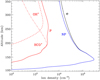 |
Fig. 11 Comparison of various ion density profiles based on our solar minimum model calculations, including the total ion (or electron) density profile (denoted as “e”), the summed density profile of all non-protonated ions (denoted as “NP”), the summed density profile of all protonated ions (denoted as “P”), as well as the density profiles of the two most abundant protonated species (OH+ and HCO+). |
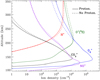 |
Fig. 12 Comparison of the ion density profiles in the dayside Venusian ionosphere at solar minimum, for several representative species between our nominal model run with protonated species (solid) and another model run without (dashed). |
5 Discussion
In Sect. 4, we elaborate on the impacts of Coulomb interaction and protonation on the structure of the dayside Venusian ionosphere, which are especially prominent at high altitudes. These two processes could certainly explain some of the model discrepancies between the present study and FS01. For instance, our model  abundance in the topside ionosphere is substantially higher than that of FS01, which is likely due to the missing of an important high-altitude
  source in the early model without protonated species (in particular OH+), as addressed above. As another instance, our model density profiles for several light species such as H+ and C+ are enhanced in the topside ionosphere relative to those of FS01. This is evidently linked to the redistribution of group I ions by suppressed ion diffusion when Coulomb collisions are included. However, this same argument does not explain our model density profiles for N+ and O+(4S), which are reduced rather than enhanced when compared to FS01. Meanwhile, the difference in the topside C+ distribution appears to be too large to be fully attributed to Coulomb collisions.
The above facts, along with some other model discrepancies addressed in Sect. 3, call for extra interpretations related to the difference in microscopic parameterization, chemistry of non-protonated species, incident solar EUV and SXR irradiance, as well as background atmospheric structure implemented by different authors. Rather than providing an interpretation for each difference one by one (which is impossible because the required information from FS01 is sometimes incomplete for drawing a firm conclusion), we highlight several aspects of our model calculations which are crucial for understanding some discrepancies between the two studies.
First of all, we note that the difference in the background atmosphere between this study and the early one is usually not a concern because both calculations are based on the VTS3 model atmosphere (Hedin et al. 1983). One obvious distinction is that we use a substantially lower O2 mixing ratio by an order of magnitude than FS01. For most species, the O2 abundance in the atmosphere has insignificant influences. However, O2 is critically relevant to the production of  , a species not modeled in FS01, via two proton transfer reactions (see Appendix D.1.11). Of more interest is the abundance of C in the Venusian upper atmosphere, for which our model predicts a much higher density than FS01 at all altitudes (see Fig. 8). This is evidently linked to the difference in the underlying O2 concentration between the two studies as the destruction of C occurs mainly via its reaction with O2:

It is worth emphasizing that the above feature does not affect much the model C+ distribution because C+ is mainly produced via the dissociative ionization of CO2 and CO rather than the direct ionization of C (see Appendix D.1.2).
Secondly, another distinction in the background atmosphere between the two studies is related to the imposed H2 distribution. Despite that the same bottom boundary condition of 0.1 ppm for the H2 mixing ratio is used by both studies, the high-altitude H2 abundance in our model is substantially higher than that of FS01. For instance, the H2 abundance that we use is higher by more than a factor of 10 near 300 km. Such a discrepancy is due to the remarkably different molecular diffusion coefficients used by different authors (see Appendix A for more details). The aforementioned distinction in background H2 strongly affects the degree of protonation in the model ionosphere, which further causes the model distinction in the topside abundances of some species provided that they rapidly react with H2. In particular, we expect that enhanced chemical destruction of O+(4S) and N+ via two reactions,

in our model accounts for the high-altitude depletion of these two species as compared to FS01. Such an effect is sufficiently strong to offset the “expected” accumulation in the topside ionosphere by Coulomb collisions.
Thirdly, here we report a large difference in C+ distribution between the two studies (see Fig. 6), with our C+ peak density higher than the old result by a factor of nearly 4. In addition to Coulomb collisions, the above distinction should also be linked to the different photochemical schemes for non-protonated species adopted in different models. In FS01, C+ production is mainly driven by the photoionization of atmospheric C; whereas in our model, this channel is negligible at all altitudes and accounts for only a small fraction of C+ production via the dissociative photoionization of CO2 when it is column-integrated. The above comparison is particularly instructive by noting that the C distribution in our model is enhanced over that of FS01 (see above). We speculate that C+ production via the dissociative ionization of CO2 was either completely ignored or seriously underestimated in FS01. Similarly, the neglect of CO2 photodissociation in FS01 that produces C and O2, which is a fairly recent finding (Lu et al. 2014), should contribute to the difference in the model C distribution.
Fourthly, the difference in NO distribution between the two studies is also large (see Fig. 8), with the peak density predicted by our model smaller than the early result by a large factor of more than 6. A careful examination suggests that one key is the different rate constants for the dominant NO production channel:

which is spin forbidden. The rate constant of 1.7 × 10⁻¹⁶ cm3 s−1 used by FS01 is in reality the upper limit. The rate constant that we use is based on the more recent compilation of Lo et al. (2020) and is as low as 2 × 10⁻¹⁷ cm3 s−1 near the NO peak. This fact partly accounts for the difference in NO distribution between the two studies seen in Fig. 8. The remaining difference is likely linked to the role of NO destruction via photoionization (see Appendix D.2.5). While FS01 reported two reactions:

as important NO destruction channels (which we also find to be important), they probably overlooked the importance of NO photoionization. Our model suggests it to be the dominant destruction channel both near the bottom boundary and above 210 km. Since NO has the lowest ionization potential (9.26 eV) among all species considered in this study, less energetic solar photons (especially in the Lyα band, shortward of the NO threshold wavelength of 1340 Å) can penetrate deep into the Venusian atmosphere and cause substantial NO ionization. An enhanced NO ionization in our model also contributes to an enhanced NO+ abundance below the V2 peak (see Fig. 7). This gains further support from the observation that the maximum model discrepancies in NO and NO+ between the two models are collocated near 130 km, which could be due to either the difference in the input solar EUV and SXR spectrum or the difference in the NO photoionization cross-section.
Finally, we remind that the recent laboratory measurements of Tenewitz et al. (2018) indicate a negligible rate constant for:

and a rate constant for

which is an order of magnitude lower than the old value from Fehsenfeld et al. (1970). The rate constants for the above two reactions are crucial for interpreting the ionospheric composition on both Venus and Mars because they determine the distribution of the dominant species,  . We use the old rate constants reported more than 50 yr ago as our nominal choice because models using these values reproduce better the mass spectrometer measurements of the Martian ionosphere (Fox et al. 2021).
The same rate constants were also adopted by FS01. Despite this, the new results cannot be disregarded and it is worthwhile to investigate how the model results would be affected by using the new rate constants instead of the old ones.
For this purpose, we performed another model run keeping every model setup identical to the nominal model except that the Tenewitz et al. (2018)’s rate constants for  are used. A comparison of the two models is depicted in Fig. 13. The discrepancy between them is compatible with our expectation. The nominal model predicts a significantly lower
  abundance and higher O+ (4S) and
  abundances in the Venusian ionosphere, due to the high rate constants for both channels of the
  reaction imposed in the nominal calculations. Such model differences are more evident at low altitudes where the effect of chemistry is prominent. Another important species that is significantly affected is HCO+, as one of the two most abundant protonated species in our model. Figure 13 reveals a significantly enhanced HCO+ distribution at low altitudes when the Tenewitz et al. (2018) rate constants are used, which is linked to the production of HCO+ from
  via
via

The model differences for the remaining species are usually small, such as NO+ (not shown in the figure) with a small enhancement linked to the production of NO+ from  (see above). When column-integrated over the simulation regime, the
  and O+(4S) abundances are reduced by 30% and 12% when we use the Tenewitz et al. (2018)’s rate constants, whereas the
  abundance is enhanced by a factor of nearly 7 and the HCO+ abundance enhanced by more than 80%, respectively. The total ion (or electron) content is also slightly reduced when the Tenewitz et al. (2018)’s rate constants are adopted because
  is more rapidly destructed via DR than
  (see Table C.2).
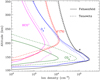 |
Fig. 13 Comparison of various ion density profiles based on our solar minimum model calculations, along with the total ion (or electron) density profile (denoted as “e”). The solid lines show our nominal model results with the |

6 Concluding remarks
Venus contains an ionosphere that should in many aspects resemble the ionosphere of Mars, as both planets possess a  dominated atmosphere with a similar neutral composition. This certainly implies a comparable ionospheric composition on the two planets. However, photochemical modeling studies of the Venusian ionosphere are far less mature than similar studies made for Mars. In particular, recent modelings of the Martian ionosphere usually incorporate the effect of protonation because the presence of even a small amount of hydrogen in the background atmosphere would trigger the formation of a variety of protonated species (Benna et al. 2015). Via such an analogy to Mars, we would expect protonation to be important on Venus as well, which serves as one of the main objectives of the present study.
We construct a detailed one-dimensional model of the day-side Venusian ionosphere including both photochemistry and diffusion. For the photochemistry, the model incorporates more than 50 ion and neutral species and more than 500 two-body chemical reactions, more than 60 spontaneous and collisional deexcitation processes, along with more than 500 photon and photoelectron impact channels, whereas for diffusion, the model takes into account both ion-neutral and ion-ion Coulomb collisions. Secondary ionization by photoelectrons is included with the aid of a two-stream kinetic model that solves the photoelectron fluxes in the upward and downward directions separately. In the model, we consider as many as 17 protonated species and, for the first time, we evaluate how the structure of the Venusian ionosphere is affected by protonation. For the purposes of this study, we focus on the solar minimum condition for which the effect of protonation is expected to be more prominent.
In general, the net effect of protonation is to diverge the ionization flow into more channels via a series of proton transfer reactions along the direction of low to high proton affinities for parent neutrals (Fox 2015). Our model predicts OH+ and HCO+ as the two most abundant protonated species: the former has a peak density of 2.1 × 103 cm−3 at 272 km and the latter has a peak density of 3.0 × 103 cm−3 at 195 km, respectively. When column-integrated, OH+ is mainly produced via the reaction between O+ (4S) and H2 and destructed via its reaction with O. For HCO+, it is produced via a variety of channels and as a terminal species, it is lost primarily via DR. Despite that protonated ions occupy only a small fraction of the total ionospheric plasma, these ions do exert an appreciable impact on the Venusian ionosphere. In particular, the distribution of  is significantly enhanced at high altitudes, where it can be efficiently produced via the reaction between O and OH+.
As another main objective of the present study, we also evaluate the role of Coulomb collisions, which are not included in many existing photochemical models for the ionospheres of both Mars and Venus. In general, Coulomb collisions suppress ion diffusion and as a consequence, the total ion (or electron) density in the topside ionosphere is enhanced as compared to the case with ion-neutral diffusion only. Such a scenario was proposed for Mars by Matta et al. (2013) and is shown here for Venus as well. However, a scrutinization of individual ion species reveals a more complicated scenario. For species preferentially produced at low altitudes (denoted as group II ions here), their abundances in the topside Venusian ionosphere are in reality reduced rather than enhanced when Coulomb collisions are considered. A matter of particular interest lies in the fact that Coulomb collisions influence the topside ionosphere not only directly by modifying diffusion, but also indirectly by modifying chemistry. The latter further indicates that, contrary to one’s intuitive expectation, the effect of Coulomb collisions extends beyond ions to minor neutrals owing to the coupled nature of the Venusian upper atmosphere and ionosphere.
Our model results highlight the importance of protonation and Coulomb interaction in a proper characterization of the Venusian ionosphere. The combination of these two processes may account for many of the differences in the model ion distribution between this study and the early benchmark study of FS01. However, other factors such as the difference in microscopic parameterization, chemistry of non-protonated species, incident solar irradiance, as well as background atmospheric structure may also contribute to various aspects of the model difference. In particular, a higher H2 abundance that we use leads to a substantial depletion of O+(4S) and N+ in the topside ionosphere compared to FS01 as both species react rapidly with H2. Our model predictions made here remain to be confirmed by future Venus orbital missions planned to perform in situ measurements of the ionosphere at the accuracy of the Neutral Gas and Ion Mass Spectrometer (NGIMS) measurements made on board the Mars Atmosphere and Volatile Evolution (MAVEN) spacecraft (Jakosky et al. 2015).
Acknowledgements
This work is supported by the B-type Strategic Priority Program No. XDB41000000 funded by the Chinese Academy of Sciences (CAS). The authors also acknowledge supports from the National Natural Science Foundation of China through grants 42274218 to XSW, 42105120 to HG, and 42304166 to YTC, as well as the Guangdong Basic and Applied Basic Research Foundation through grant 2023A1515011987.
Appendix A Binary diffusion coefficients and neutral polarizabilities
Information on the molecular diffusion coefficients for various neutral species within a background CO2 or O gas are provided in Table A.1, adapted from the compilation of Mason & Marrero (1970) and García Muñoz (2007). For some of the binary gas mixtures with no reported diffusion coefficients, one approach is to compute the coefficients based on the conventional kinetic theory assuming hard sphere approximation as adopted in FS01. However, such an approach usually leads to large discrepancies from available laboratory measurements or more robust calculations (e.g. Ern & Giovangigli 1997). For instance, using the hard sphere radii reported in Fox & Hać (2014), we estimate that for Ar, O2, H2, and H as representative species, their molecular diffusion coefficients predicted by the kinetic theory are significantly smaller than those listed in Table A.1 by a factor of ~ 200–500 within a background CO2 gas. For the above reason, the molecular diffusion coefficients for binary gas mixtures not reported by Mason & Marrero (1970) and García Muñoz (2007) are assumed to be identical to those for similar gas mixtures throughout our ionospheric modeling. In particular, for ground- and excited-state C, for excited-state N and O, as well as for CH, NH, and OH, their diffusion coefficients within a background O gas are taken to be identical to the N–O diffusion coefficient reported by García Muñoz (2007), and their diffusion coefficients within a background CO2 gas are taken to be identical to the O–CO2 diffusion coefficient also reported by García Muñoz (2007).
In contrast, for each ion species, the binary ion-neutral and ion-ion diffusion coefficients are straightforwardly computed based on the kinetic theory. The polarizabilities required for computing the former, which are detailed in Table A.2, are adapted from the Kinetic Database for Astrochemistry (KIDA, Wakelam et al. 2015) available at https://kida.astrochem-tools.org, except for the Ar polarizability taken as 1.49 × 10⁻²⁴ cm3 from Asher et al. (1995).
Compilation of molecular diffusion coefficients*
Compilation of polarizabilities
Appendix B Photon and photoelectron impact cross-sections
A complicated network of photon and photoelectron impact processes much more thorough than previous modeling efforts is implemented in this study. The photoabsorption cross-sections, required for computing the attenuation of the incident solar EUV and SXR spectrum, are exclusively based on the compilation of Heays et al. (2017). We consider in our calculations photoabsorption by the 10 background species only, whereas photoabsorption by the extra minor neutrals solved self-consistently by the model is neglected for simplicity. Information on the detailed photodissociation and photoionization processes for each species, either background or minor, is provided in Table B.1 along with the respective threshold energies and reference sources for cross-sections.
For photoelectron impact processes, the cross-sections are significantly updated from our previous compilation in Cui et al. (2011), as detailed in Table B.2. Under many circumstances, electronic excitation of atmospheric molecules by photoelectron impact is followed by pre-dissociation. The photoelectron energy degradation associated with these processes is naturally accounted for in the model, but their contributions to the production of neutral fragments are neglected because they are of minor importance to ionospheric chemistry and also because the corresponding pre-dissociation fractions are mostly unknown.
Compilation of photon impact processes*
Compilation of photoelectron impact processes*
Appendix C Chemical reactions, spontaneous emission and collisional quenching processes
A complicated chemical network is implemented in our calculations. For completeness, we provide detailed information on the ion-neutral reactions in Table C.1, recombination reactions in Table C.2, neutral-neutral reactions in Table C.3, spontaneous emission processes in Table C.4, as well as collisional quenching processes (by both neutrals and electrons) in Table C.5, respectively. For most channels, the rate constants are based on the recent compilation of Lo et al. (2020) and Vuitton et al. (2019), with additional channels from the KIDA database (Wakelam et al. 2015) along with a number of other references. In all tables, “hv” stands for photons and “e” stands for ionospheric electrons in general (to be distinguished from “e*” denoting specifically photoelectrons, see Appendix D).
Compilation of ion-neutral reactions*
Compilation of recombination reactions*
Compilation of neutral-neutral reactions*
Compilation of spontaneous emission processes*
Compilation of collisional quenching processes*
Appendix D Detailed chemical budget for each species in our model
For reference, we list in Tables D.1 and D.2 various production and destruction channels for each ion and minor neutral species included in our calculations, with the numbers in parentheses referring to their fractional contributions to the total chemical production and destruction rates integrated over the model altitude range of 100–350 km. Only those channels with fractional contributions above 1% are tabulated. Some channels, though making negligible contributions to the total chemical budget, are found to be important over specific altitude ranges. Therefore we also display, for each species, the detailed chemical scheme as a function of the altitude, in terms of the fractional contributions of all important channels to the total production or destruction rate. This allows the relative importance of each channel to be displayed over a common scale and hence more easily identified than the conventional plot showing the absolute production or loss rate.
Appendix D.1 Chemical pathways for various ion species
We show in Figures D.1–D.13 the fractional contributions of important chemical pathways for a range of ion species in our model. Only those channels, either production or destruction, with fractional contributions above 10% at any given altitude within the simulation regime are indicated. A detailed description of the chemical scheme for each species is provided below.
Compilation of ion chemical pathways*
Appendix D.1.1 Ar+ and ArH+
The abundance of Ar+ is mainly controlled by production via the photoionization and photoelectron impact ionization of Ar in the background atmosphere and destruction via two reactions:
 (R1)
(R1)
 (R2)
(R2)
Among the Ar+ production channels, our model indicates that photoionization is important at essentially all altitudes within the simulation regime, whereas photoelectron impact ionization is of comparable importance from the bottom boundary up to 140 km, above which its importance declines rapidly with increasing altitude. For Ar+ destruction, R1 and R2 are dominant below and above 200 km, respectively.
As protonated Ar, ArH+ is mainly produced via R2 and destructed via its proton transfer reactions with CO2, O, and H2:
 (R3)
(R3)
 (R4)
(R4)
 (R5)
(R5)
with R3 dominating below 165 km, R5 above 300 km, and R4 in between.
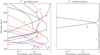 |
Fig. D.1 The fractional contributions to the total C+ production (left) and destruction (right) rates from various chemical channels in the dayside Venusian ionosphere based on our solar minimum model calculations. Only those channels with factional contributions at any given altitude above 10% are indicated. The red, blue, and black lines stand for photon and photoelectron impact processes, as well as two-body chemical reactions, respectively. Channel notations (left): 1. CO2 + hv → C+ + O+ (4S) + O + 2e; 2. CO2 + hv → C+ + O2 + e; 3. CO + hv → C+ + O + e; 4. C + hv → C+ + e; 5. CO2 + e* → C+ + O2 + 2e; 6. CO2 + e* → C+ + O+(4S) + O + 3e; 7. He+ + CO → C+ + O + He; 8. CH+ + H → C+ + H2; 9. |

Appendix D.1.2 C+, CH+, and 
The detailed chemical scheme for C+ is provided in Figure D.1, which appears to be very complicated. According to our calculations, C+ can be effectively produced via the dissociative ionization of CO2 and CO by solar photons and photoelectrons in many different channels, of which the most important one is
 (R6)
(R6)
dominating near the V2 peak and accounting for 60% of the column-integrated C+ production (see Table D.1). Below 130 km, the dissociative photoelectron impact ionization of CO2:
 (R7)
(R7)
prevails. With increasing altitude, C+ production via ion-neutral reactions becomes more important such as
 (R8)
(R8)
dominating at 200–260 km.
As for C+ destruction, the leading channel below 240 km is its reaction with CO2, mainly proceeding as
 (R9)
(R9)
At higher altitudes, C+ is more effectively destructed via
 (R10)
(R10)
We also include CH+, which is protonated C, in our model, showing that the bulk of CH+ production occurs via the proton transfer reaction:
 (R11)
(R11)
a channel that dominates from the bottom boundary up to 240 km. At higher altitudes (up to 275 km), another proton transfer reaction:
 (R12)
(R12)
produces CH+ more rapidly than R11. The dominant CH+ destruction channel is its reaction with CO2:
 (R13)
(R13)
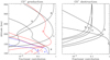 |
Fig. D.2 Similar to Figure D.1 for CO+ production (left) and destruction (right). The red, blue, and black lines stand for photon and photoelectron impact processes, as well as two-body chemical reactions, respectively. Channel notations (left): 1. CO2 + hv → CO+ + O+ (4S) + 2e; 2. CO2 + hv → CO+ + O + e; 3. CO + hv → CO+ + e; 4. CO2 + e* → CO+ + O + 2e; 5. CO2 + e* → CO+ + O+ (4S) + 3e; 6. C+ + CO2 → CO+ + CO; 7. O+ (2D) + CO → CO+ + O; 8. CH+ + O → CO+ + H; 9. |


CO+ + H → H+ + CO.
below 180 km, whereas at higher altitudes, its reaction with O becomes more important, proceeding either as
 (R14)
(R14)
or as
 (R15)
(R15)
with equal probability (Vuitton et al. 2019). CH+ DR is unimportant except above 240 km. CH+ can be further converted to  via the reaction:
 (R16)
(R16)
a process that is the primary  production channel above 130 km. Proton transfer from HCO+ is more effective just below the V2 peak, proceeding as
 (R17)
(R17)
 destruction occurs mainly via its reactions with O and CO2 in the background atmosphere:
 (R18)
(R18)
 (R19)
(R19)
of which the former mainly operates above 160 km and the latter below. CH+ DR is unimportant except above 250 km.
Appendix D.1.3 CO+ and 
Both  and CO+ are relatively abundant in the dayside Venusian ionosphere. Their chemical schemes are illustrated in Figures D.2 and D.3, revealing that many different channels are responsible for their production and destruction.
The production of CO+ occurs mainly via the photoionization of CO, which dominates at 140-170 km, along with two reactions: R9 dominating below and
 (R20)
(R20)
above (up to at least 270 km). R20 is exothermic by 2.92 eV, whereas the analogous reaction O+ (4S) + CO → CO+ + O is not allowed at typical ionospheric temperatures because it is endothermic by 0.40 eV. The destruction of CO+ below 190 km is mainly via its charge exchange reaction with CO2:
 (R21)
(R21)
whereas CO+ DR becomes dominant at high altitudes.
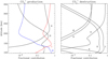 |
Fig. D.3 Similar to Figure D.1 for |


 is primarily produced via the photoionization (above 130 km) and photoelectron impact ionization (below 130 km) of CO2. Two charge exchange reactions are substantial over a broad altitude range from 170 km to 270 km, which are R21 and
 (R22)
(R22)
Similarly, R22 is exothermic by 3.16 eV, whereas the analogous reaction  is endothermic by 0.16 eV and hence not viable. For
  destruction, the leading pathway is its reaction with O proceeding either as
 (R23)
(R23)
or as
 (R24)
(R24)
over the lower half portion of the simulation regime. In particular, R23 destructs  more efficiently than R24 by 70% according to their difference in rate constant (Fehsenfeld et al. 1970), but be cautious that the recent laboratory measurements of Tenewitz et al. (2018) suggest instead that the
  reaction occurs exclusively via channel R23 (see Section 5 for more details). The contribution from
  DR is of minor importance except above 230 km.
Appendix D.1.4 H+,  , and
, and 
The chemical scheme for H+ is depicted in Figure D.4. Below 155 km, the charge exchange reaction:
 (R25)
(R25)
is the dominant H+ production pathway, whereas at higher altitudes, it is surpassed by another charge exchange reaction:
 (R26)
(R26)
Photoionization of H or H2 is of negligible importance. The destruction of H+ is fairly simple, dominated by the inverse reaction of R26:
 (R27)
(R27)
above 180 km and
 (R28)
(R28)
below. Charge exchange reactions R26 and R27 both proceed at typical ionospheric temperatures because the absolute enthalpy difference between the reactants and products is only 0.02 eV.
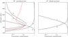 |
Fig. D.4 Similar to Figure D.1 for H+ production (left) and destruction (right). The red and black lines stand for photon impact processes and two-body chemical reactions, respectively. Channel notations (left): 1. H + hv → H+ + e; 2. |

 is effectively produced via the photoionization and photoelectron impact ionization of H2, dominating above and below 140 km, respectively, along with the charge exchange reaction:
 (R29)
(R29)
which is particularly important over a narrow altitude range centered at 210 km. R29 is exothermic by 1.51 eV, whereas the analogous reaction  is not allowed because it is endothermic by 1.81 eV. The bulk of
  destruction occurs via two proton transfer reactions:
 (R30)
(R30)
below 160 km and
 (R31)
(R31)
above. The  reaction can also proceed in other channels, which are less important. For
  , several proton transfer reactions account for the bulk of its production, including
 (R32)
(R32)
 (R33)
(R33)
Among them R32 dominates below 150 km and above 250 km, whereas R33 dominates in between. Important  destruction channels include its reactions with CO2 and O:
 (R34)
(R34)
 (R35)
(R35)
R34 dominates below 170 km whereas R35 dominates above.  DR is unimportant except above 290 km.
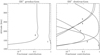 |
Fig. D.5 Similar to Figure D.1 for OH+ production (left) and destruction (right). Channel notations (left): 1. O+ (4S) + H2 → OH+ + H; 2. O+ (2D) + H2 → OH+ + H. Channel notations (right): 1. OH+ + CO2 → HOCO+ + O; 2. |

Appendix D.1.5 OH+, H2O+, and H3O+
Despite that the Venusian atmosphere is known to be dry (thus no H2O vapor is imposed in our background atmosphere), photochemistry can produce a fair amount of water group ions at ionospheric altitudes (see Figure 5). By analogy, Fox et al. (2015) also predicted the presence of the same set of species in the Martian ionosphere in their model of no vertical transport of tropospheric water vapor to high altitudes.
Our model calculations for Venus suggest that for OH+, the dominant production channel is
 (R36)
(R36)
at all altitudes and the dominant destruction channel is its reaction with O:
 (R37)
(R37)
above 165 km and with CO2:
 (R38)
(R38)
below, as depicted in Figure D.5. DR is insignificant except near and above 300 km.
The conversion from OH+ by consuming ambient H2:
 (R39)
(R39)
is the leading channel producing H2O+, except below 130 km where the proton transfer reaction:
 (R40)
(R40)
prevails. H2O+ is predominantly destructed via
 (R41)
(R41)
below 185 km, whereas DR prevails at high altitudes in several channels (Vuitton et al. 2019).
A similar conversion from H2O+ in the presence of H2:
 (R42)
(R42)
is responsible for producing essentially all H3O+ in the Venusian ionosphere, a process that is exclusively balanced by DR indicating that H3+ is a terminal species.
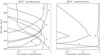 |
Fig. D.6 Similar to Figure D.1 for HCO+ production (left) and destruction (right). Channel notations (left): 1. HOCO+ + CO → HCO+ + CO2; 2. HOCO+ + O → HCO+ + O2; 3. OH+ + CO → HCO+ + O; 4. CO+ + H2 → HCO+ + H; 5. |

HOC+ + H2 → HCO+ + H2. Channel notations (right): 1. HCO+ + O2 → HOCO+ + O; 2. HCO+ + e → CO + H; 3. HCO+ + C → CH+ + CO.
Appendix D.1.6 HCO+, HOC+, and HOCO+
CO has two protonated species: HCO+ and HOC+. The former has a lower heat of formation than the latter per particle, and is thus thermodynamically more stable.
As shown in Figure D.6, HCO+ production is rather complicated with several channels making significant contributions including R28 and
 (R43)
(R43)
 (R44)
(R44)
 (R45)
(R45)
The relative importance of each channel varies with the altitude depending on the abundances of the reactants. HCO+ is a terminal species because it is mainly destructed via DR.
Our model indicates that HOC+ is nearly exclusively produced via
 (R46)
(R46)
and destructed via its proton transfer reactions with several background species such as CO2 and CO:
 (R47)
(R47)
 (R48)
(R48)
of which the former dominates below 185 km and the latter above up to 220 km. At higher altitudes, DR destructs HOC+ most efficiently. HOC+ cannot be directly isomerized to form HCO+ at typical ionospheric temperatures because of a large barrier of 1.61 eV required for direct isomerization (Mladenović & Schmatz 1998). The presence of “catalytic” species is necessary such as CO in R48.
HOCO+, as protonated CO2 and the most massive ion species in our model, is produced mainly via R38 at 180–250 km and
 (R49)
(R49)
both below (down to at least 120 km) and above. It is destructed rapidly by reacting with CO (R43) below 135 km and O:
 (R50)
(R50)
above (up to 240 km where DR becomes more important).
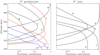 |
Fig. D.7 Similar to Figure D.1 for N+ production (left) and destruction (right). The red, blue, and black lines stand for photon and photoelectron impact processes, as well as two-body chemical reactions, respectively. Channel notations (left): 1. N2 + hv → N+ + N + e; 2. N + hv → N+ + e; 3. N2 + e* → N+ + N + 2e; 4. N2 + e* → N+ + N+ + 3e; 5. O+(2D) + N → N+ + O; 6. |


Appendix D.1.7 N+ and 
As shown in Figure D.7, N+ is predominantly produced via the ionization of atmospheric N2 and N by solar photons and photoelectrons. The dissociative ionization of N2 prevails from the lower boundary to 165 km, mainly via photoelectron impact below 130 km and via photon impact above. The direct ionization of N becomes more important at higher altitudes. When column-integrated over the entire simulation regime, N2 photoionization produces 5 times more N+ than N photoionization (see Table D.1). N+ destruction occurs via its reactions with CO2, CO, and H2:
 (R51)
(R51)
 (R52)
(R52)
 (R53)
(R53)
Among them, R51 dominates below 190 km, R53 above 220 km, and R52 in between.
The chemical scheme for  is shown in Figure D.8, revealing that
  production is dominated by the photoionization and photoelectron impact ionization of N2 above and below 130 km. Two extra reactions are also important:
 (R54)
(R54)
at 200–230 km and
 (R55)
(R55)
above 280 km. In particular, R54 is exothermic by 1.36 eV whereas the analogous  reaction is endothermic by 1.96 eV.
  is rapidly destructed via its reactions with CO2 and O:
 (R56)
(R56)
 (R57)
(R57)
R56 dominates below 180 km and R57 at 180–230 km.  DR prevails at higher altitudes, which mainly produces two excited-state N(2D) atoms (Dutuit et al. 2013).
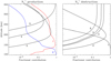 |
Fig. D.8 Similar to Figure D.1 for |


Appendix D.1.8 NH+,  , and N2H+
In the presence of hydrogen in the background atmosphere (see Figure 1), N-containing neutrals could be protonated, resulting in the formation of NH+,  , and N2H+.
NH+ is predominantly produced via
 (R58)
(R58)
at all altitudes and destructed via
 (R59)
(R59)
above 150 km. At lower altitudes, NH+ is more rapidly destructed via its reaction with CO2, of which several distinct channels are possible (Lo et al. (2020)).
Once produced, NH+ could be further converted to  by consuming H2:
 (R60)
(R60)
R60 is the dominant  production channel above 160 km and is supplemented by the proton transfer reaction:
 (R61)
(R61)
that dominates at lower altitudes.  is mainly destructed via its reaction with O:
 (R62)
(R62)
below 220 km (down to 110 km) and via DR above.
N2H+ is efficiently produced via the reaction:
 (R63)
(R63)
at nearly all altitudes. However, the contributions from two proton transfer reactions:
 (R64)
(R64)
 (R65)
(R65)
become important at 180–240 km. N2H+ destruction occurs mainly via
 (R66)
(R66)
below 180 km and
 (R67)
(R67)
at higher altitudes up to 240 km where DR starts to prevail.
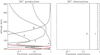 |
Fig. D.9 Similar to Figure D.1 for NO+ production (left) and destruction (right). The red and black lines stand for photon impact processes and two-body chemical reactions, respectively. Channel notations (left): 1. NO + hv → NO+ + e; 2. |


Appendix D.1.9 NO+ and HNO+
The chemical scheme for NO+ in the dayside Venusian ionosphere, as displayed in Figure D.9, is complicated. NO+ is efficiently produced via several channels, each dominant at a specific altitude range within our simulation regime. In particular, the leading channel is
 (R68)
(R68)
below 230 km (down to 120 km) and
 (R69)
(R69)
above. The contribution from R57 is also significant near 200 km. NO photoionization and an extra atom-interchange reaction:
 (R70)
(R70)
are in general negligible but could be important near the bottom boundary. The destruction of NO+, as a terminal species, occurs exclusively via DR, which produces three times more excited-state N(2D) than ground-state N (Vuitton et al. 2019).
For protonated NO, HNO+, its production scheme is complicated in that many ion-neutral chemical channels make significant contributions, including
 (R71)
(R71)
below 125 km,
 (R72)
(R72)
at 125–185 km, and
 (R73)
(R73)
at higher altitudes. HNO+ is mainly destructed via DR above 200 km. At lower altitudes, its destruction is dominated by the proton transfer reaction:
 (R74)
(R74)
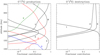 |
Fig. D.10 Similar to Figure D.1 for ground-state O+(4S) production (left) and destruction (right). The red, blue, green, and black lines stand for photon impact, photoelectron impact, and spontaneous emission processes, as well as two-body chemical reactions, respectively. Channel notations (left): 1. CO2 + hv → O+(4S) + CO + e; 2. O + hv → O+(4S) + e; 3. CO2 + e* → O+(4S) + CO + 2e; 4. |


Appendix D.1.10 O+(4S), O+(2D), and O+(2P)
In the topside Venusian ionosphere above 220 km, O+(4S) dominates over  and becomes the most abundant species (see Figure 5). In our model, we consider not only ground-state O+(4S), but also excited-state O+(2D) and O+(2P).
The production of O+(4S) is dominated by the charge exchange reaction R24 below 175 km, the direct photoionization of O at 175–220 km, another charge exchange reaction R27 at 220–300 km, as well as the collisional quenching of excited-state O+ (2D) by electrons at higher altitudes. Below 200 km, O+ (4S) is mainly destructed via its reaction with CO2:
 (R75)
(R75)
At higher altitudes, the importance of R75 declines rapidly and two extra reactions: R26 and R36, also as important H+ and OH+ production channels (see above), destruct O+ (4S) much more rapidly. The chemical scheme outlined above is depicted in Figure D.10 for reference.
For O+ (2D) and O+ (2P), they are mainly produced via the ionization of O by solar photons and photoelectrons, with the former dominant above 130 km and the latter below. The most important destruction channel for O+(2D) is R22 below 170 km, R20 at 170–220 km, as well as
 (R76)
(R76)
and collisional quenching by electrons at even higher altitudes. Some of these channels also serve as important chemical sources for the respective product ions (see above). For O+(2P), it is predominantly destructed via its reaction with CO2:
 (R77)
(R77)
below 160 km. O+(2P) can also be destructed effectively via spontaneous emission, a process that dominates at high altitudes. Upon emission, the bulk of O+(2P) decays to lower excited-state O+(2D) rather than to ground-state O+(4S) (Seaton & Osterbrock 1957). However, spontaneous emission is unimportant for O+(2D) destruction at all altitudes. For reference, the detailed chemical schemes for the two excited-state species are depicted in Figures D.11 and D.12.
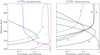 |
Fig. D.11 Similar to Figure D.1 for excited-state O+(2D) production (left) and destruction (right). The red, blue, green, and black lines stand for photon impact, photoelectron impact, and spontaneous emission processes, as well as two-body chemical reactions, respectively. Channel notations (left): 1. O + hv→ O+(2D) + e; 2. O + e* → O+(2D) + 2e; 3. O+(2P) + O → O+(2D) + O; 4. O+(2P) → O+(2D) + hv. Channel notations (right): 1. |

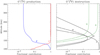 |
Fig. D.12 Similar to Figure D.1 for excited-state O+(2P) production (left) and destruction (right). The red, blue, green, and black lines stand for photon impact, photoelectron impact, and spontaneous emission processes, as well as two-body chemical reactions, respectively. Channel notations (left): 1. O + hv→ O+(2P) + e; 2. O + e* → O+(2P) + 2e. Channel notations (right): 1. |

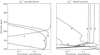 |
Fig. D.13 Similar to Figure D.1 for |


Appendix D.1.11  and
and 
 is the most abundant ionospheric species near the V2 peak, which is mainly produced via R23 and R75. These two channels are of comparable importance below 170 km, above which the importance of both channels declines rapidly with increasing altitude, making R37 to prevail all the way up to the top boundary.
  is primarily destructed via DR in several channels, some of which are well known to drive substantial O escape on present-day Mars (e.g. Fox & Hać 2009, 2014; Lillis et al. 2017) but not on Venus due to a larger gravitational barrier (Gu et al. 2021). Several extra reactions are also important
  destruction channels near the bottom boundary, including R70 and
 (R78)
(R78)
 (R79)
(R79)
The chemical scheme for  is displayed in Figure D.13.
As protonated O2,  is also included in our model, showing that, over a broad altitude range from 160 km to 250 km, the dominant production channel is the proton transfer reaction:
 (R80)
(R80)
whereas at both higher and lower altitudes, another proton transfer reaction:
 (R81)
(R81)
becomes more important. The main destruction channel of  is its proton transfer reactions with CO2 and O:
 (R82)
(R82)
 (R83)
(R83)
mainly operating below and above 160 km, respectively. DR is unimportant except above 250 km.
Appendix D.1.12 He+ and HeH+
He+ is exclusively produced via the photoionization (above 130 km) and photoelectron impact ionization (below 130 km) of He in the background atmosphere. It is effectively destructed via its reaction with CO2:
 (R84)
(R84)
below 165 km and R8 above. He+ reaction with O is negligible due to the exceedingly low rate constant despite that it is exothermic by 11 eV (FS01).
For HeH+, the proton transfer reaction:
 (R85)
(R85)
accounts for essentially all its production within our simulation regime. HeH+ destruction mainly occurs via its reaction with H2:
 (R86)
(R86)
except at 130–170 km where DR prevails.
Appendix D.2 Chemical pathways for various minor neutral species
We show in Figures D.14–D.20 the fractional contributions of important chemical pathways for a range of minor neutral species in our model. Only those channels, either production or destruction, with fractional contributions above 10% at any given altitude within the simulation regime are indicated. A detailed description of the chemical scheme for each species is provided below.
Compilation of minor neutral chemical pathways*
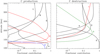 |
Fig. D.14 Similar to Figure D.1 for C production (left) and destruction (right). The red, blue, green, and black lines stand for photon impact, photoelectron impact, and spontaneous emission processes, as well as two-body chemical reactions, respectively. Channel notations (left): 1. CO2 + hν → C + O2; 2. CO + hν → C + O; 3. CO2 + e* → O+ + O+ + C + 3e; 4. C+ + CO2 → CO+ + C; 5. CO+ + e → C + O; 6. CH+ + e → C + H; 7. C(1D) + e → C + e. Channel notations (right): 1. C + hν → C+ + e; 2. C + O2 → CO + O; 3. O+ (4S) + C → C+ + O; 4. OH+ + C → CH+ + O; 5. C + C → C2 + hν. |
Appendix D.2.1 C, C(1D), and C(1S)
We start with photochemically produced atomic C in the Venusian upper atmosphere, of which the chemical scheme is displayed in Figure D.14 for reference. C can be rapidly produced via the photodissociation of CO2 and CO at 130–190 km. CO2 photodissociation is operative at lower altitudes as a greater amount of energy is required to break the parent molecules. When column-integrated over the simulation regime, CO2 photodissociation produces slightly more C atoms than CO photodissociation. Below 130 km, the charge exchange reaction:
 (R87)
(R87)
prevails, whereas above 190 km, DR of several C-containing ion species (CO+ in particular) is more important than photodissociation. Unlike the situation on Mars (Lo et al. (2020)), HCO+ DR makes a tiny contribution to C production in the Venusian upper atmosphere. C is mainly destructed via its reaction with O2:
 (R88)
(R88)
below 180 km and the proton transfer reaction:
 (R89)
(R89)
at high altitudes. Meanwhile, the contributions from radiative recombination:
 (R90)
(R90)
and the proton transfer reaction R11 are appreciable at 180-240 km. The significant role played by ion-neutral chemistry on the C distribution is indicative of the coupled nature of the Venusian upper atmosphere and ionosphere.
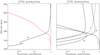 |
Fig. D.15 Similar to Figure D.1 for C(1D) production (left) and destruction (right). The red, green, and black lines stand for photon impact and spontaneous emission processes, as well as two-body chemical reactions, respectively. Channel notations (left): 1. CO + hν → C(1D) + O(1D); 2. CO+ + e → C(1D) + O. Channel notations (right): 1. C(1D) + CO2 → CO + CO; 2. C(1D) + CO → C + CO; 3. C(1D) + e → C + e; 4. C(1D) → C + hν. |
Two excited states of C are also incorporated in our model: C(lD) and C(1S). The chemical scheme for the former is shown in Figure D.15. The production of C(1D) is fairly simple, dominated by CO photolysis below 190 km and CO+ DR above. The former produces excited-state C(lD) and O(lD), whereas the latter produces excited-state C(lD) and ground-state O. CO+ DR cannot produce both C and O in excited states because such a reaction is endothermic by 0.32 eV. The collisional excitation of ground-state C by photoelectrons is negligible. The destruction of C(1D) occurs predominantly via its reaction with CO2:
 (R91)
(R91)
below 180 km and collisional quenching by electrons above. C(1D) also decays spontaneously to the ground state, but this channel is generally unimportant except above 270 km.
The production of higher excited-state C(1S) occurs mainly via CO photodissociation at 150–180 km and via collisional excitation of ground-state C by photoelectrons at both lower and higher altitudes. The former produces more C(1S) atoms than the latter in the column-integrated sense (see Table D.2). C(1S) is mainly destructed via collisional quenching by CO2 below 135 km and via spontaneous emission above, both decaying to lower excited-state C(1D). The latter is much more important than the former when column-integrated (see Table D.2).
Appendix D.2.2 N(2D) and N(2P)
We now move on to the two excited states of atomic N: N(2D) and N(2P), with detailed chemical schemes displayed in Figures D.16 and D.17. For N(2D), it is primarily produced via NO+ DR, which preferentially produces N(2D) rather than ground-state N (see Appendix D.1.9). N2 photodissociation is generally of less importance, whereas the contribution from the spontaneous emission of higher excited-state N(2P) could be significant near 175 km. N(2D) destruction occurs via a number of processes, dominated by
 (R92)
(R92)
below 150 km, collisional quenching by electrons above 190 km, and collisional quenching by CO and O in between. Collisional quenching by O can proceed in two channels of equal probability, producing either ground-state O or excited-state O(1D) (Vuitton et al. 2019). The latter channel is energetically allowed because N(2D) has a higher excitation energy (2.38 eV, Bakalian (2006)) than O(1D) (1.97 eV, Lillis et al. (2017)). Spontaneous decay of N(2D) is in general unimportant.
N(2P) is mainly produced via the photodissociation of N2 in two channels, producing, in addition to one N(2P) atom, either a ground-state N atom or a lower excited-state N(2D) atom (Fox 2007a). The collisional excitation of ground-state N by photoelectrons becomes more important below 135 km whereas  DR prevails above 260 km. N(2P) is efficiently destructed via collisional quenching by O below 140 km and via spontaneous emission above, both decaying to lower excited-state N(2D).
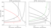 |
Fig. D.16 Similar to Figure D.1 for N(2D) production (left) and destruction (right). The red, green, and black lines stand for photon impact and spontaneous emission processes, as well as two-body chemical reactions, respectively. Channel notations (left): 1. N2 + hv → Ν + N(2D); 2. |

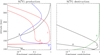 |
Fig. D.17 Similar to Figure D.1 for N(2P) production (left) and destruction (right). The red, blue, green, and black lines stand for photon impact, photoelectron impact, and spontaneous emission processes, as well as two-body chemical reactions, respectively. Channel notations (left): |


Appendix D.2.3 O(1D) and O(1S)
As depicted in Figure D.18, O(1D) can be effectively produced in the dayside Venusian upper atmosphere via several channels, of which spontaneous emission from higher excited-state O(lS) is dominant near and below the V2 peak. At higher altitudes, DR becomes more substantial, via two channels with a total branching ratio of 2/3 (Lillis et al. 2017). The photodissociation of atmospheric O2 is in general unimportant except near the bottom boundary. Destruction of O(1D) is dominated by collisional quenching by CO2 below 180 km and spontaneous decay to ground-state Ο above.
The chemical scheme for O(lS) is relatively simple, as displayed in Figure D.19. CO2 photodissociation dominates its production below 190 km, whereas  DR dominates at higher altitudes, even though the specific channel that produces O(lS) has a branching ratio of 6% only (Lillis et al. 2017). Destruction of O(lS) is dominated by spontaneous decay to lower excited-state O(1D) throughout the bulk of the simulation regime. Collisional quenching (by CO2 is negligible except near the bottom boundary.
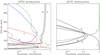 |
Fig. D.18 Similar to Figure D.1 for O(1D) production (left) and destruction (right). The red, blue, green, and black lines stand for photon impact, photoelectron impact, and spontaneous emission processes, as well as two-body chemical reactions, respectively. Channel notations (left): 1. O2 + hν → Ο + O(1D); 2. CO2 + hv → CO + O(1D); 3. Ο + e* → O(1D) + e; 4. O(1S) → O(1D) + hv; 5. 0(1S) + CO2 → O(1D) + CO2; 6. O(1S) + Ο → O(1D) + O; 7. |


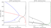 |
Fig. D.19 Similar to Figure D.1 for O(1S) production (left) and destruction (right). The red, blue, green, and black lines stand for photon impact, photoelectron impact, and spontaneous emission processes, as well as two-body chemical reactions, respectively. Channel notations (left): 1. |


Appendix D.2.4 CH, NH, and OH
In the dayside Venusian upper atmosphere, the abundances of CH, NH, and OH radicals strongly depend on the ambient H2 distribution because they are mainly produced via three similar reactions:
 (R93)
(R93)
 (R94)
(R94)
 (R95)
(R95)
Here excited-state atoms are required as reactants because the analogous reactions involving ground-state C, N, and Ο atoms are endothermic. DR of certain protonated species may also contribute substantially to radical production over restricted altitude ranges, in particular HCO+ DR that produces both OH and CH near and below the V2 peak, along with H2O+ DR that produces OH above 225 km. Furthermore, radiative association could also be important for OH production below 120 km.
All the three radicals are predominantly destructed via their reactions with O:
 (R96)
(R96)
 (R97)
(R97)
 (R98)
(R98)
except at sufficiently high altitudes where their reactions with either H or H+ start to prevail.
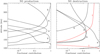 |
Fig. D.20 Similar to Figure D.1 for NO production (left) and destruction (right). The red and black lines stand for photon impact processes and two-body chemical reactions, respectively. Channel notations (left): 1. N + CO2 → NO + CO; 2. N(2D) + CO2 → NO + CO; 3. N+ + CO2 → CO+ + NO; 4. NH + O → NO + H; 5. HNO+ + e → NO + H. Channel notations (right): 1. NO + hν → N + O; 2. N + NO → N2 + O; 3. O+ + NO → NO+ + O2; 4. C + NO → CO + N; 5. H+ + NO → NO+ + H. |
Appendix D.2.5 NO
NO is an important species in the atmospheres of Earth, Mars, and Venus, because it is both chemically and radiatively active. For instance, NO plays a crucial role in the energy budget of the terrestrial upper atmosphere via its infrared emission at 5.3 µm (Kockarts 1980). According to our model, NO in the Venusian upper atmosphere can be produced via a number of channels, of which the most important one is R92, mainly operative at 135-185 km. Below 135 km, it is predominantly produced via
 (R99)
(R99)
and above 185 km, ion-neutral chemistry comes into effect. The only DR reaction that potentially produces NO is HNO+ DR, but this channel is unimportant except above 270 km due to the exceedingly low concentration of the parent protonated species (see Figure 5).
The prevailing destruction channel for NO is its reaction with N:
 (R100)
Photoionization could also be operative at certain altitudes, both near the lower boundary and above 210 km.
References
- Ambili, K. M., Babu, S. S., & Choudhary, R. K. 2019, Icarus, 321, 661 [NASA ADS] [CrossRef] [Google Scholar]
- Angel, G. C., & Samson, J. A. R. 1988, Phys. Rev. A, 38, 5578 [NASA ADS] [CrossRef] [Google Scholar]
- Asher, R. L., Bellert, D., Buthelezi, T., Lewis, V., & Brucat, P. J. 1995, Chem. Phys. Lett., 234, 113 [NASA ADS] [CrossRef] [Google Scholar]
- Bakalian, F. 2006, Icarus, 183, 69 [NASA ADS] [CrossRef] [Google Scholar]
- Benna, M., Mahaffy, P. R., Grebowsky, J. M., et al. 2015, Geophys. Res. Lett., 42, 8958 [NASA ADS] [CrossRef] [Google Scholar]
- Blaha, M., & Davis, J. 1975, Phys. Rev. A, 12, 2319 [NASA ADS] [CrossRef] [Google Scholar]
- Brace, L. H., & Kliore, A. J. 1991, Space Sci. Rev., 55, 81 [NASA ADS] [CrossRef] [Google Scholar]
- Bray, I., & Stelbovics, A. T. 1995, Adv. At. Mol. Opt. Phys., 35, 209 [NASA ADS] [CrossRef] [Google Scholar]
- Brinton, H. C., Taylor, H. A., Niemann, H. B., et al. 1980, Geophys. Res. Lett., 7, 865 [NASA ADS] [CrossRef] [Google Scholar]
- Campbell, L., Brunger, M. J., Cartwright, D. C., & Teubner, P. J. O. 2004, Planet. Space Sci., 52, 815 [NASA ADS] [CrossRef] [Google Scholar]
- Cao, Y., Cui, J., Liang, W., Wu, X., & Lu, H. 2023, AJ, 166, 264 [NASA ADS] [CrossRef] [Google Scholar]
- Chaffin, M. S., Chaufray, J. Y., Deighan, J., et al. 2018, J. Geophys. Res. (Planets), 123, 2192 [NASA ADS] [CrossRef] [Google Scholar]
- Chamberlin, P. C., Eparvier, F. G., Knoer, V., et al. 2020, Space Weather, 18, e02588 [NASA ADS] [CrossRef] [Google Scholar]
- Chen, R. H., & Nagy, A. F. 1978, J. Geophys. Res., 83, 1133 [NASA ADS] [CrossRef] [Google Scholar]
- Chung, Y. M., Lee, E. M., Masuoka, T., & Samson, J. A. R. 1993, J. Chem. Phys., 99, 885 [NASA ADS] [CrossRef] [Google Scholar]
- Coates, A. J., Frahm, R. A., Linder, D. R., et al. 2008, Planet. Space Sci., 56, 802 [Google Scholar]
- Cravens, T. E., Kliore, A. J., Kozyra, J. U., & Nagy, A. F. 1981, J. Geophys. Res., 86, 11323 [NASA ADS] [CrossRef] [Google Scholar]
- Cui, J., Galand, M., Coates, A. J., Zhang, T. L., & Müller-Wodarg, I. C. F. 2011, J. Geophys. Res. Space Phys., 116, A04321 [NASA ADS] [Google Scholar]
- Dang, T., Zhang, B., Yan, M., et al. 2023, ApJ, 945, 91 [NASA ADS] [CrossRef] [Google Scholar]
- de Bergh, C., Bezard, B., Owen, T., et al. 1991, Science, 251, 547 [NASA ADS] [CrossRef] [Google Scholar]
- Donahue, T. M., & Hartle, R. E. 1992, Geophys. Res. Lett., 19, 2449 [NASA ADS] [CrossRef] [Google Scholar]
- Donahue, T. M., Hoffman, J. H., Hodges, R. R., & Watson, A. J. 1982, Science, 216, 630 [NASA ADS] [CrossRef] [Google Scholar]
- Dujardin, G., Besnard, M. J., Hellner, L., & Malinovitch, Y. 1987, Phys. Rev. A, 35, 5012 [NASA ADS] [CrossRef] [Google Scholar]
- Dutuit, O., Carrasco, N., Thissen, R., et al. 2013, ApJS, 204, 20 [NASA ADS] [CrossRef] [Google Scholar]
- Ern, A., & Giovangigli, V. 1997, Linear Algebra Appl., 250, 289 [CrossRef] [Google Scholar]
- Fedorova, A., Bertaux, J.-L., Betsis, D., et al. 2018, Icarus, 300, 440 [NASA ADS] [CrossRef] [Google Scholar]
- Fehsenfeld, F. C., Dunkin, D. B., & Ferguson, E. E. 1970, Planet. Space Sci., 18, 1267 [NASA ADS] [CrossRef] [Google Scholar]
- Feldman, P. D., Steffl, A. J., Parker, J. W., et al. 2011, Icarus, 214, 394 [NASA ADS] [CrossRef] [Google Scholar]
- Fjeldbo, G., Seidel, B., Sweetnam, D., & Howard, T. 1975, J. Atmos. Sci., 32, 1232 [NASA ADS] [CrossRef] [Google Scholar]
- Fox, J. L. 1988, Planet. Space Sci., 36, 37 [NASA ADS] [CrossRef] [Google Scholar]
- Fox, J. L. 2007a, Icarus, 192, 296 [NASA ADS] [CrossRef] [Google Scholar]
- Fox, J. L. 2007b, J. Geophys. Res. Planets, 112, E04S02 [Google Scholar]
- Fox, J. L. 2008, J. Geophys. Res. Planets, 113, E11001 [NASA ADS] [CrossRef] [Google Scholar]
- Fox, J. L. 2015, Icarus, 252, 366 [NASA ADS] [CrossRef] [Google Scholar]
- Fox, J. L., & Bougher, S. W. 1991, Space Sci. Rev., 55, 357 [CrossRef] [Google Scholar]
- Fox, J. L., & Hac´, A. B. 2009, Icarus, 204, 527 [NASA ADS] [CrossRef] [Google Scholar]
- Fox, J. L., & Hac´, A. B. 2014, Icarus, 228, 375 [NASA ADS] [CrossRef] [Google Scholar]
- Fox, J. L., & Paxton, L. J. 2005, J. Geophys. Res. Space Phys., 110, A01311 [NASA ADS] [CrossRef] [Google Scholar]
- Fox, J. L., & Sung, K. Y. 2001, J. Geophys. Res., 106, 21305 [NASA ADS] [CrossRef] [Google Scholar]
- Fox, J. L., Galand, M. I., & Johnson, R. E. 2008, Space Sci. Rev., 139, 3 [NASA ADS] [CrossRef] [Google Scholar]
- Fox, J. L., Benna, M., Mahaffy, P. R., & Jakosky, B. M. 2015, Geophys. Res. Lett., 42, 8977 [NASA ADS] [CrossRef] [Google Scholar]
- Fox, J. L., Benna, M., McFadden, J. P., Jakosky, B. M., & Maven Ngims Team 2021, Icarus, 358, 114186 [NASA ADS] [CrossRef] [Google Scholar]
- Futaana, Y., Stenberg Wieser, G., Barabash, S., & Luhmann, J. G. 2017, Space Sci. Rev., 212, 1453 [NASA ADS] [CrossRef] [Google Scholar]
- García Muñoz, A. 2007, Planet. Space Sci., 55, 1414 [CrossRef] [Google Scholar]
- Gérard, J. C., Bougher, S. W., López-Valverde, M. A., et al. 2017, Space Sci. Rev., 212, 1617 [CrossRef] [Google Scholar]
- Gibson, J. C., Green, M. A., Trantham, K. W., et al. 1999, J. Phys. B At. Mol. Phys., 32, 213 [NASA ADS] [CrossRef] [Google Scholar]
- Gillmann, C., Way, M. J., Avice, G., et al. 2022, Space Sci. Rev., 218, 56 [NASA ADS] [CrossRef] [Google Scholar]
- Girazian, Z., Withers, P., Häusler, B., et al. 2015, Planet. Space Sci., 117, 146 [CrossRef] [Google Scholar]
- Grinspoon, D. H. 1993, Nature, 363, 428 [CrossRef] [Google Scholar]
- Grondin, R., Loison, J.-C., & Hickson, K. M. 2016, J. Phys. Chem. A, 120, 4838 [NASA ADS] [CrossRef] [Google Scholar]
- Gu, H., Cui, J., Niu, D., & Yu, J. 2021, MNRAS, 501, 2394 [NASA ADS] [CrossRef] [Google Scholar]
- Guan, L., Jiang, P., Zhang, G., et al. 2021, A&A, 647, A127 [NASA ADS] [CrossRef] [EDP Sciences] [Google Scholar]
- Han, Q., Fraenz, M., Wei, Y., et al. 2020, Earth Planet. Phys., 4, 73 [Google Scholar]
- Hartle, R. E., Donahue, T. M., Grebowsky, J. M., & Mayr, H. G. 1996, J. Geophys. Res., 101, 4525 [NASA ADS] [CrossRef] [Google Scholar]
- Heavens, N. G., Kleinböhl, A., Chaffin, M. S., et al. 2018, Nat. Astron., 2, 126 [Google Scholar]
- Heays, A. N., Bosman, A. D., & van Dishoeck, E. F. 2017, A&A, 602, A105 [NASA ADS] [CrossRef] [EDP Sciences] [Google Scholar]
- Hedin, A. E., Niemann, H. B., Kasprzak, W. T., & Seiff, A. 1983, J. Geophys. Res., 88, 73 [NASA ADS] [CrossRef] [Google Scholar]
- Hensley, K., Withers, P., Girazian, Z., et al. 2020, J. Geophys. Res. Space Phys., 125, e27167 [NASA ADS] [CrossRef] [Google Scholar]
- Herman, J. R., Hartle, R. E., & Bauer, S. J. 1971, Planet. Space Sci., 19, 443 [NASA ADS] [CrossRef] [Google Scholar]
- Herron, J. T. 1999, J. Phys. Chem. Ref. Data, 28, 1453 [NASA ADS] [CrossRef] [Google Scholar]
- Hickson, K. M., Loison, J.-C., Bourgalais, J., et al. 2015, ApJ, 812, 107 [NASA ADS] [CrossRef] [Google Scholar]
- Hickson, K. M., Loison, J.-C., Lique, F., & Klos, J. 2016, J. Phys. Chem. A, 120, 2504 [NASA ADS] [CrossRef] [Google Scholar]
- Huebner, W. F., & Mukherjee, J. 2015, Planet. Space Sci., 106, 11 [Google Scholar]
- Husain, D., & Norris, P. E. 1979, Faraday Discuss. Chem. Soc., 67, 273 [CrossRef] [Google Scholar]
- Husain, D., & Newton, D. P. 1982, J. Chem. Soc., Faraday Trans., 78, 51 [CrossRef] [Google Scholar]
- Imamura, T., Toda, T., Tomiki, A., et al. 2011, Earth Planets Space, 63, 493 [Google Scholar]
- Itikawa, Y. 2002, J. Phys. Chem. Ref. Data, 31, 749 [Google Scholar]
- Itikawa, Y. 2006, J. Phys. Chem. Ref. Data, 35, 31 [NASA ADS] [CrossRef] [Google Scholar]
- Itikawa, Y. 2009, J. Phys. Chem. Ref. Data, 38, 1 [NASA ADS] [CrossRef] [Google Scholar]
- Itikawa, Y. 2015, J. Phys. Chem. Ref. Data, 44, 013105 [NASA ADS] [CrossRef] [Google Scholar]
- Ivanov-Kholodny, G. S., Kolosov, M. A., Savich, N. A., et al. 1979, Icarus, 39, 209 [NASA ADS] [CrossRef] [Google Scholar]
- Jackman, C. H., Garvey, R. H., & Green, A. E. S. 1977, J. Geophys. Res., 82, 5081 [NASA ADS] [CrossRef] [Google Scholar]
- Jakosky, B. M., Lin, R. P., Grebowsky, J. M., et al. 2015, Space Sci. Rev., 195, 3 [CrossRef] [Google Scholar]
- Johnstone, C. P., Güdel, M., Lammer, H., & Kislyakova, K. G. 2018, A&A, 617, A107 [NASA ADS] [CrossRef] [EDP Sciences] [Google Scholar]
- Keating, G. M., Nicholson, J. Y., & Lake, L. R. 1980, J. Geophys. Res., 85, 7941 [NASA ADS] [CrossRef] [Google Scholar]
- Kliore, A. J., & Mullen, L. F. 1989, J. Geophys. Res., 94, 13339 [NASA ADS] [CrossRef] [Google Scholar]
- Kliore, A., Levy, G. S., Cain, D. L., Fjeldbo, G., & Rasool, S. I. 1967, Science, 158, 1683 [NASA ADS] [CrossRef] [Google Scholar]
- Kliore, A. J., Woo, R., Armstrong, J. W., Patel, I. R., & Croft, T. A. 1979, Science, 203, 765 [NASA ADS] [CrossRef] [Google Scholar]
- Kliore, A. J., Moroz, V. I., & Keating, G. M. 1985, Adv. Space Res., 5 [Google Scholar]
- Knudsen, W. C., & Miller, K. L. 1992, J. Geophys. Res., 97, 17165 [NASA ADS] [CrossRef] [Google Scholar]
- Knudsen, W. C., Spenner, K., Miller, K. L., & Novak, V. 1980, J. Geophys. Res., 85, 7803 [NASA ADS] [CrossRef] [Google Scholar]
- Kockarts, G. 1980, Geophys. Res. Lett., 7, 137 [NASA ADS] [CrossRef] [Google Scholar]
- Krasnopolsky, V. A. 2019, Icarus, 321, 62 [NASA ADS] [CrossRef] [Google Scholar]
- Krasnopolsky, V. A., & Gladstone, G. R. 2005, Icarus, 176, 395 [NASA ADS] [CrossRef] [Google Scholar]
- Kumar, S., & Hunten, D. M. 1974, J. Geophys. Res., 79, 2529 [NASA ADS] [CrossRef] [Google Scholar]
- Laher, R. R., & Gilmore, F. R. 1990, J. Phys. Chem. Ref. Data, 19, 277 [NASA ADS] [CrossRef] [Google Scholar]
- Laporta, V., Cassidy, C. M., Tennyson, J., & Celiberto, R. 2012, Plasma Sources Sci. Technol., 21, 045005 [NASA ADS] [CrossRef] [Google Scholar]
- Lavvas, P., Galand, M., Yelle, R. V., et al. 2011, Icarus, 213, 233 [NASA ADS] [CrossRef] [Google Scholar]
- Lawrence, G. M. 1972, J. Chem. Phys., 57, 5616 [NASA ADS] [CrossRef] [Google Scholar]
- Lias, S. G., Liebman, J. F., & Levin, R. D. 1984, J. Phys. Chem. Ref. Data, 13, 695 [CrossRef] [Google Scholar]
- Lillis, R. J., Deighan, J., Fox, J. L., et al. 2017, J. Geophys. Res. Space Phys., 122, 3815 [NASA ADS] [CrossRef] [Google Scholar]
- Lo, D. Y., Yelle, R. V., & Lillis, R. J. 2020, Icarus, 352, 114001 [NASA ADS] [CrossRef] [Google Scholar]
- Lo, D. Y., Yelle, R. V., Lillis, R. J., & Deighan, J. I. 2021, Icarus, 360, 114371 [NASA ADS] [CrossRef] [Google Scholar]
- Lu, Z., Chang, Y. C., Yin, Q.-Z., Ng, C. Y., & Jackson, W. M. 2014, Science, 346, 61 [NASA ADS] [CrossRef] [Google Scholar]
- Lu, H. Y., Cao, J. B., Zhang, T. L., Fu, H. S., & Ge, Y. S. 2015, Phys. Plasmas, 22, 062902 [NASA ADS] [CrossRef] [Google Scholar]
- Luhmann, J. G. 1986, Space Sci. Rev., 44, 241 [NASA ADS] [CrossRef] [Google Scholar]
- Ma, Y. J., Nagy, A. F., Russell, C. T., et al. 2013, J. Geophys. Res. Space Phys., 118, 321 [NASA ADS] [CrossRef] [Google Scholar]
- Mahajan, K. K., & Mayr, H. G. 1989, Geophys. Res. Lett., 16, 1477 [NASA ADS] [CrossRef] [Google Scholar]
- Mahajan, K. K., Mayr, H. G., Brace, L. H., & Cloutier, P. A. 1989, Geophys. Res. Lett., 16, 759 [NASA ADS] [CrossRef] [Google Scholar]
- Martinis, C. R., Wilson, J. K., & Mendillo, M. J. 2003, J. Geophys. Res. Space Phys., 108, 1383 [NASA ADS] [Google Scholar]
- Mason, E. A., & Marrero, T. R. 1970, Adv. At. Mol. Phys., 6, 155 [NASA ADS] [CrossRef] [Google Scholar]
- Masuoka, T. 1994, Phys. Rev. A, 50, 3886 [NASA ADS] [CrossRef] [Google Scholar]
- Masuoka, T., & Nakamura, E. 1993, Phys. Rev. A, 48, 4379 [NASA ADS] [CrossRef] [Google Scholar]
- Matta, M., Withers, P., & Mendillo, M. 2013, J. Geophys. Res. Space Phys., 118, 2681 [NASA ADS] [CrossRef] [Google Scholar]
- McElroy, M. B. 1968, J. Atmos. Sci., 25, 574 [NASA ADS] [CrossRef] [Google Scholar]
- Mendillo, M., Lollo, A., Withers, P., et al. 2011, J. Geophys. Res. Space Phys., 116, A11303 [Google Scholar]
- Mladenović, M., & Schmatz, S. 1998, J. Chem. Phys., 109, 4456 [CrossRef] [Google Scholar]
- Nagy, A. F., Liu, S. C., Donahue, T. M., Atreya, S. K., & Banks, P. M. 1975, Geophys. Res. Lett., 2, 83 [NASA ADS] [CrossRef] [Google Scholar]
- Nagy, A. F., Cravens, T. E., Smith, S. G., Taylor, H. A., & Brinton, H. C. 1980, J. Geophys. Res., 85, 7795 [NASA ADS] [CrossRef] [Google Scholar]
- Nahar, S. N. 1999, ApJS, 120, 131 [NASA ADS] [CrossRef] [Google Scholar]
- Niemann, H. B., Kasprzak, W. T., Hedin, A. E., Hunten, D. M., & Spencer, N. W. 1980, J. Geophys. Res., 85, 7817 [NASA ADS] [CrossRef] [Google Scholar]
- Nuñez-Reyes, D., & Hickson, K. M. 2017, Chem. Phys. Lett., 687, 330 [CrossRef] [Google Scholar]
- Nuñez-Reyes, D., & Hickson, K. M. 2018, J. Phys. Chem. A, 122, 4002 [CrossRef] [Google Scholar]
- Okabe, H. 1978, Photochemistry of small molecules (New York: Wiley) [Google Scholar]
- Pancheshnyi, S., Biagi, S., Bordage, M. C., et al. 2012, Chem. Phys., 398, 148 [NASA ADS] [CrossRef] [Google Scholar]
- Pätzold, M., Häusler, B., Bird, M. K., et al. 2007, Nature, 450, 657 [CrossRef] [Google Scholar]
- Peter, K., Pätzold, M., Molina-Cuberos, G., et al. 2014, Icarus, 233, 66 [NASA ADS] [CrossRef] [Google Scholar]
- Petrignani, A., van der Zande, W. J., Cosby, P. C., et al. 2005, J. Chem. Phys., 122, 014302 [NASA ADS] [CrossRef] [Google Scholar]
- Phillips, J. L., Luhmann, J. G., & Russell, C. T. 1985, Adv. Space Res., 5, 173 [NASA ADS] [CrossRef] [Google Scholar]
- Phillips, J. L., Luhmann, J. G., Knudsen, W. C., & Brace, L. H. 1988, J. Geophys. Res., 93, 3927 [NASA ADS] [CrossRef] [Google Scholar]
- Ralchenko, Y., Janev, R. K., Kato, T., et al. 2008, Atomic Data Nuclear Data Tables, 94, 603 [NASA ADS] [CrossRef] [Google Scholar]
- Rampino, S., & Suleimanov, Y. V. 2016, J. Phys. Chem. A, 120, 9887 [NASA ADS] [CrossRef] [Google Scholar]
- Register, D. F., Trajmar, S., & Srivastava, S. K. 1980, Phys. Rev. A, 21, 1134 [NASA ADS] [CrossRef] [Google Scholar]
- Richards, P. G., & Torr, D. G. 1988, J. Geophys. Res., 93, 4060 [NASA ADS] [CrossRef] [Google Scholar]
- Rosén, S., Peverall, R., Larsson, M., et al. 1998, Phys. Rev. A, 57, 4462 [CrossRef] [Google Scholar]
- Samson, J. A. R., Masuoka, T., & Pareek, P. N. 1985, J. Chem. Phys., 83, 5531 [NASA ADS] [CrossRef] [Google Scholar]
- Samson, J. A. R., Masuoka, T., Pareek, P. N., & Angel, G. C. 1987, J. Chem. Phys., 86, 6128 [NASA ADS] [CrossRef] [Google Scholar]
- Sawada, T., Sellin, D. L., & Green, A. E. S. 1972, J. Geophys. Res., 77, 4819 [NASA ADS] [CrossRef] [Google Scholar]
- Schofield, K. 1978, J. Photochem., 9, 55 [CrossRef] [Google Scholar]
- Seaton, M. J., & Osterbrock, D. E. 1957, ApJ, 125, 66 [CrossRef] [Google Scholar]
- Song, M.-Y., Yoon, J.-S., Cho, H., et al. 2019, J. Phys. Chem. Ref. Data, 48, 043104 [NASA ADS] [CrossRef] [Google Scholar]
- Spenner, K., Knudsen, W. C., Whitten, R. C., et al. 1981, J. Geophys. Res., 86, 9170 [NASA ADS] [CrossRef] [Google Scholar]
- Stevefelt, J., Boulmer, J., & Delpech, J. F. 1975, Phys. Rev. A, 12, 1246 [NASA ADS] [CrossRef] [Google Scholar]
- Stolte, W. C., He, Z. X., Cutler, J. N., Lu, Y., & Samson, J. A. R. 1998, Atomic Data Nuclear Data Tables, 69, 171 [NASA ADS] [CrossRef] [Google Scholar]
- Stone, S. W., Yelle, R. V., Benna, M., et al. 2020, Science, 370, 824 [NASA ADS] [CrossRef] [Google Scholar]
- Straub, H. C., Renault, P., Lindsay, B. G., Smith, K. A., & Stebbings, R. F. 1995, Phys. Rev. A, 52, 1115 [NASA ADS] [CrossRef] [Google Scholar]
- Strömholm, C., Semaniak, J., Rosén, S., et al. 1996, Phys. Rev. A, 54, 3086 [CrossRef] [Google Scholar]
- Tabata, T., Shirai, T., Sataka, M., & Kubo, H. 2006, Atomic Data Nuclear Data Tables, 92, 375 [NASA ADS] [CrossRef] [Google Scholar]
- Tawara, H., & Kato, T. 1987, Atomic Data Nuclear Data Tables, 36, 167 [CrossRef] [Google Scholar]
- Tawara, H., Itikawa, Y., Nishimura, H., & Yoshino, M. 1990, J. Phys. Chem. Ref. Data, 19, 617 [CrossRef] [Google Scholar]
- Taylor, H. A., Brinton, H. C., Bauer, S. J., et al. 1979a, Science, 205, 96 [NASA ADS] [CrossRef] [Google Scholar]
- Taylor, H. A., Brinton, H. C., Bauer, S. J., et al. 1979b, Science, 203, 752 [NASA ADS] [CrossRef] [Google Scholar]
- Taylor, H. A., Brinton, H. C., Bauer, S. J., et al. 1980, J. Geophys. Res., 85, 7765 [NASA ADS] [CrossRef] [Google Scholar]
- Taylor, H. A., Niemann, H. B., Mayr, H. G., et al. 1984, J. Geophys. Res., 89, 10669 [CrossRef] [Google Scholar]
- Tenewitz, J. E., Lê, T., Martinez, O., et al. 2018, J. Chem. Phys., 148, 084305 [NASA ADS] [CrossRef] [Google Scholar]
- Terada, N., Shinagawa, H., Tanaka, T., Murawski, K., & Terada, K. 2009, J. Geophys. Res. Space Phys., 114, A09208 [NASA ADS] [CrossRef] [Google Scholar]
- Theis, R. F., Brace, L. H., Elphic, R. C., & Mayr, H. G. 1984, J. Geophys. Res., 89, 1477 [CrossRef] [Google Scholar]
- Thomas, L. D., & Nesbet, R. K. 1975, Phys. Rev. A, 12, 2378 [NASA ADS] [CrossRef] [Google Scholar]
- Tian, C., & Vidal, C. R. 1999, Phys. Rev. A, 59, 1955 [NASA ADS] [CrossRef] [Google Scholar]
- Tripathi, K. R., Choudhary, R. K., Ambili, K. M., & Imamura, T. 2023, J. Geophys. Res. Planets, 128, e2023JE007768 [NASA ADS] [CrossRef] [Google Scholar]
- Tsang, S. M. E., Coates, A. J., Jones, G. H., et al. 2015, Planet. Space Sci., 113, 385 [CrossRef] [Google Scholar]
- Verner, D. A., Ferland, G. J., Korista, K. T., & Yakovlev, D. G. 1996, ApJ, 465, 487 [Google Scholar]
- Vuitton, V., Yelle, R. V., Klippenstein, S. J., Hörst, S. M., & Lavvas, P. 2019, Icarus, 324, 120 [CrossRef] [Google Scholar]
- Wakelam, V., Loison, J. C., Herbst, E., et al. 2015, ApJS, 217, 20 [NASA ADS] [CrossRef] [Google Scholar]
- Wang, Y., Zatsarinny, O., & Bartschat, K. 2013, Phys. Rev. A, 87, 012704 [NASA ADS] [CrossRef] [Google Scholar]
- Wang, Y., Zatsarinny, O., & Bartschat, K. 2014, Phys. Rev. A, 89, 062714 [NASA ADS] [CrossRef] [Google Scholar]
- Williams, J. F., & Allen, L. J. 1989, J. Phys. B At. Mol. Phys., 22, 3529 [NASA ADS] [CrossRef] [Google Scholar]
- Witasse, O., Cravens, T., Mendillo, M., et al. 2008, Space Sci. Rev., 139, 235 [NASA ADS] [CrossRef] [Google Scholar]
- Wu, Z., Li, T., Zhang, X., Li, J., & Cui, J. 2020, Nat. Commun., 11, 614 [Google Scholar]
- Wu, X., Cui, J., Niu, D., Ren, Z., & Wei, Y. 2021, ApJ, 923, 29 [NASA ADS] [CrossRef] [Google Scholar]
- Yoon, J.-S., Song, M.-Y., Han, J.-M., et al. 2008, J. Phys. Chem. Ref. Data, 37, 913 [CrossRef] [Google Scholar]
- Zammit, M. C., Savage, J. S., Fursa, D. V., & Bray, I. 2017, Phys. Rev. A, 95, 022708 [NASA ADS] [CrossRef] [Google Scholar]
- Zatsarinny, O., Wang, Y., & Bartschat, K. 2014, Phys. Rev. A, 89, 022706 [NASA ADS] [CrossRef] [Google Scholar]
All Tables
All Figures
|
Fig. 1 Structure of the underlying Venusian upper atmosphere used in our model calculations, appropriate for the dayside averaged condition at solar minimum. Left: density profiles of 10 background species (CO2, O, CO, N2, N, He, O2, H2, H, and Ar). For comparison, we also show the H2 density profile adopted by FS01 for solar minimum, which presents the most pronounced distinction from our choice among all species. Right: neutral, ion, and electron temperature profiles (denoted as Tn, Ti, and Te, respectively). |
| In the text | |
|
Fig. 2 Solar EUV and SXR spectrum (at the top of the Venusian atmosphere) used in our solar minimum model calculations over the wavelength range of 0.05–189.95 nm with a resolution of 0.1 nm. |
| In the text | |
|
Fig. 3 Photoelectron energy spectra in the upward (solid) and downward (dashed) directions in the dayside Venusian ionosphere, at two representative altitudes as indicated in the figure legend. Notable photoelectron signatures, such as the He II peak and aluminum edge, are clearly visible. |
| In the text | |
|
Fig. 4 Comparison of ion production rate and ionization efficiency for several selected species. Left: ion production rate profiles associated with primary (solid) and secondary (dashed) ionization. Right: respective ionization efficiency profiles. Primary ionization refers to photoionization and secondary ionization refers to photoelectron impact ionization, respectively. The ionization efficiency is defined as the ratio of the secondary to primary ion production rate. |
| In the text | |
|
Fig. 5 Dayside averaged density profiles of various ion species in the Venusian ionosphere based on our solar minimum model calculations. All species display well-defined peak structures, usually superimposed by secondary peaks at lower altitudes though typically manifest as shoulders. The thick solid line in the upper left panel represents the electron distribution inferred from charge neutrality. |
| In the text | |
|
Fig. 6 Comparison of the electron density distribution between this study (appropriate for a SZA of 60° and a 10.7 cm solar radio index of 80 SFU) and various measurements. The solid circles are for the model density profile, the red symbols are for the VEx RO measurements covering a narrow SZA interval of 50°–60° and all at solar minimum, the blue symbols are for the Akatsuki RO measurements covering wider ranges of both SZA and 10.7 cm solar radio index, whereas the green symbols are extracted from the empirical model of Theis et al. (1984) based on the PVO in-situ measurements at solar maximum. Numbers starting with “S” and “F” refer to the corresponding values of the SZA (in degree) and 10.7 cm solar radio index (in SFU). “Smax” stands for “solar maximum.” The dates when the MEx and Akatsuki RO experiments were made are indicated in the figure legend for reference. |
| In the text | |
|
Fig. 7 Comparison of the ion density profiles at solar minimum between this study (solid) and FS01 (dashed). |
| In the text | |
|
Fig. 8 Dayside averaged density profiles of various minor neutral species based on our solar minimum model calculations, all displaying well-defined layer structures. A comparison for some species between this study (solid) and FS01 (dashed) is also indicated in the left panel. |
| In the text | |
|
Fig. 9 Comparison between two solar minimum model runs, one with ion-neutral (IN) collisions only (dashed) and the other one with both ion-neutral and ion-ion (II) Coulomb collisions (solid). The black lines show the total ion density profiles obtained by the two model runs, whereas the red and blue lines correspond to the density profiles of the group I and II ions, respectively. The former includes all ion species with peak altitudes above 200 km and the latter includes the remaining species. |
| In the text | |
|
Fig. 10 Comparison of various time constants. Left: comparison of the ion diffusion time constant (τdiff) and ion chemical destruction time constant (τchem) for several selected species, where τdiff includes the contributions from both ion-neutral collisions and ion-ion Coulomb collisions. Right: comparison of the ion-neutral collision time constant (τin) and ion-ion Coulomb collision time constant (τii) for the same species. All time constants are based on our solar minimum calculations appropriate for the dayside averaged condition. |
| In the text | |
|
Fig. 11 Comparison of various ion density profiles based on our solar minimum model calculations, including the total ion (or electron) density profile (denoted as “e”), the summed density profile of all non-protonated ions (denoted as “NP”), the summed density profile of all protonated ions (denoted as “P”), as well as the density profiles of the two most abundant protonated species (OH+ and HCO+). |
| In the text | |
|
Fig. 12 Comparison of the ion density profiles in the dayside Venusian ionosphere at solar minimum, for several representative species between our nominal model run with protonated species (solid) and another model run without (dashed). |
| In the text | |
|
Fig. 13 Comparison of various ion density profiles based on our solar minimum model calculations, along with the total ion (or electron) density profile (denoted as “e”). The solid lines show our nominal model results with the |
| In the text | |
|
Fig. D.1 The fractional contributions to the total C+ production (left) and destruction (right) rates from various chemical channels in the dayside Venusian ionosphere based on our solar minimum model calculations. Only those channels with factional contributions at any given altitude above 10% are indicated. The red, blue, and black lines stand for photon and photoelectron impact processes, as well as two-body chemical reactions, respectively. Channel notations (left): 1. CO2 + hv → C+ + O+ (4S) + O + 2e; 2. CO2 + hv → C+ + O2 + e; 3. CO + hv → C+ + O + e; 4. C + hv → C+ + e; 5. CO2 + e* → C+ + O2 + 2e; 6. CO2 + e* → C+ + O+(4S) + O + 3e; 7. He+ + CO → C+ + O + He; 8. CH+ + H → C+ + H2; 9. |
| In the text | |
|
Fig. D.2 Similar to Figure D.1 for CO+ production (left) and destruction (right). The red, blue, and black lines stand for photon and photoelectron impact processes, as well as two-body chemical reactions, respectively. Channel notations (left): 1. CO2 + hv → CO+ + O+ (4S) + 2e; 2. CO2 + hv → CO+ + O + e; 3. CO + hv → CO+ + e; 4. CO2 + e* → CO+ + O + 2e; 5. CO2 + e* → CO+ + O+ (4S) + 3e; 6. C+ + CO2 → CO+ + CO; 7. O+ (2D) + CO → CO+ + O; 8. CH+ + O → CO+ + H; 9. |
| In the text | |
|
Fig. D.3 Similar to Figure D.1 for |
| In the text | |
|
Fig. D.4 Similar to Figure D.1 for H+ production (left) and destruction (right). The red and black lines stand for photon impact processes and two-body chemical reactions, respectively. Channel notations (left): 1. H + hv → H+ + e; 2. |
| In the text | |
|
Fig. D.5 Similar to Figure D.1 for OH+ production (left) and destruction (right). Channel notations (left): 1. O+ (4S) + H2 → OH+ + H; 2. O+ (2D) + H2 → OH+ + H. Channel notations (right): 1. OH+ + CO2 → HOCO+ + O; 2. |
| In the text | |
|
Fig. D.6 Similar to Figure D.1 for HCO+ production (left) and destruction (right). Channel notations (left): 1. HOCO+ + CO → HCO+ + CO2; 2. HOCO+ + O → HCO+ + O2; 3. OH+ + CO → HCO+ + O; 4. CO+ + H2 → HCO+ + H; 5. |
| In the text | |
|
Fig. D.7 Similar to Figure D.1 for N+ production (left) and destruction (right). The red, blue, and black lines stand for photon and photoelectron impact processes, as well as two-body chemical reactions, respectively. Channel notations (left): 1. N2 + hv → N+ + N + e; 2. N + hv → N+ + e; 3. N2 + e* → N+ + N + 2e; 4. N2 + e* → N+ + N+ + 3e; 5. O+(2D) + N → N+ + O; 6. |
| In the text | |
|
Fig. D.8 Similar to Figure D.1 for |
| In the text | |
|
Fig. D.9 Similar to Figure D.1 for NO+ production (left) and destruction (right). The red and black lines stand for photon impact processes and two-body chemical reactions, respectively. Channel notations (left): 1. NO + hv → NO+ + e; 2. |
| In the text | |
|
Fig. D.10 Similar to Figure D.1 for ground-state O+(4S) production (left) and destruction (right). The red, blue, green, and black lines stand for photon impact, photoelectron impact, and spontaneous emission processes, as well as two-body chemical reactions, respectively. Channel notations (left): 1. CO2 + hv → O+(4S) + CO + e; 2. O + hv → O+(4S) + e; 3. CO2 + e* → O+(4S) + CO + 2e; 4. |
| In the text | |
|
Fig. D.11 Similar to Figure D.1 for excited-state O+(2D) production (left) and destruction (right). The red, blue, green, and black lines stand for photon impact, photoelectron impact, and spontaneous emission processes, as well as two-body chemical reactions, respectively. Channel notations (left): 1. O + hv→ O+(2D) + e; 2. O + e* → O+(2D) + 2e; 3. O+(2P) + O → O+(2D) + O; 4. O+(2P) → O+(2D) + hv. Channel notations (right): 1. |
| In the text | |
|
Fig. D.12 Similar to Figure D.1 for excited-state O+(2P) production (left) and destruction (right). The red, blue, green, and black lines stand for photon impact, photoelectron impact, and spontaneous emission processes, as well as two-body chemical reactions, respectively. Channel notations (left): 1. O + hv→ O+(2P) + e; 2. O + e* → O+(2P) + 2e. Channel notations (right): 1. |
| In the text | |
|
Fig. D.13 Similar to Figure D.1 for |
| In the text | |
|
Fig. D.14 Similar to Figure D.1 for C production (left) and destruction (right). The red, blue, green, and black lines stand for photon impact, photoelectron impact, and spontaneous emission processes, as well as two-body chemical reactions, respectively. Channel notations (left): 1. CO2 + hν → C + O2; 2. CO + hν → C + O; 3. CO2 + e* → O+ + O+ + C + 3e; 4. C+ + CO2 → CO+ + C; 5. CO+ + e → C + O; 6. CH+ + e → C + H; 7. C(1D) + e → C + e. Channel notations (right): 1. C + hν → C+ + e; 2. C + O2 → CO + O; 3. O+ (4S) + C → C+ + O; 4. OH+ + C → CH+ + O; 5. C + C → C2 + hν. |
| In the text | |
|
Fig. D.15 Similar to Figure D.1 for C(1D) production (left) and destruction (right). The red, green, and black lines stand for photon impact and spontaneous emission processes, as well as two-body chemical reactions, respectively. Channel notations (left): 1. CO + hν → C(1D) + O(1D); 2. CO+ + e → C(1D) + O. Channel notations (right): 1. C(1D) + CO2 → CO + CO; 2. C(1D) + CO → C + CO; 3. C(1D) + e → C + e; 4. C(1D) → C + hν. |
| In the text | |
|
Fig. D.16 Similar to Figure D.1 for N(2D) production (left) and destruction (right). The red, green, and black lines stand for photon impact and spontaneous emission processes, as well as two-body chemical reactions, respectively. Channel notations (left): 1. N2 + hv → Ν + N(2D); 2. |
| In the text | |
|
Fig. D.17 Similar to Figure D.1 for N(2P) production (left) and destruction (right). The red, blue, green, and black lines stand for photon impact, photoelectron impact, and spontaneous emission processes, as well as two-body chemical reactions, respectively. Channel notations (left): |
| In the text | |
|
Fig. D.18 Similar to Figure D.1 for O(1D) production (left) and destruction (right). The red, blue, green, and black lines stand for photon impact, photoelectron impact, and spontaneous emission processes, as well as two-body chemical reactions, respectively. Channel notations (left): 1. O2 + hν → Ο + O(1D); 2. CO2 + hv → CO + O(1D); 3. Ο + e* → O(1D) + e; 4. O(1S) → O(1D) + hv; 5. 0(1S) + CO2 → O(1D) + CO2; 6. O(1S) + Ο → O(1D) + O; 7. |
| In the text | |
|
Fig. D.19 Similar to Figure D.1 for O(1S) production (left) and destruction (right). The red, blue, green, and black lines stand for photon impact, photoelectron impact, and spontaneous emission processes, as well as two-body chemical reactions, respectively. Channel notations (left): 1. |
| In the text | |
|
Fig. D.20 Similar to Figure D.1 for NO production (left) and destruction (right). The red and black lines stand for photon impact processes and two-body chemical reactions, respectively. Channel notations (left): 1. N + CO2 → NO + CO; 2. N(2D) + CO2 → NO + CO; 3. N+ + CO2 → CO+ + NO; 4. NH + O → NO + H; 5. HNO+ + e → NO + H. Channel notations (right): 1. NO + hν → N + O; 2. N + NO → N2 + O; 3. O+ + NO → NO+ + O2; 4. C + NO → CO + N; 5. H+ + NO → NO+ + H. |
| In the text | |
Current usage metrics show cumulative count of Article Views (full-text article views including HTML views, PDF and ePub downloads, according to the available data) and Abstracts Views on Vision4Press platform.
Data correspond to usage on the plateform after 2015. The current usage metrics is available 48-96 hours after online publication and is updated daily on week days.
Initial download of the metrics may take a while.