| Issue |
A&A
Volume 685, May 2024
|
|
|---|---|---|
| Article Number | A152 | |
| Number of page(s) | 8 | |
| Section | Planets and planetary systems | |
| DOI | https://doi.org/10.1051/0004-6361/202245773 | |
| Published online | 20 May 2024 | |
Solar wind effect on the multi-fluid plasma expansion in the Venusian upper ionosphere
1
Institut für Theoretische Physik IV, Ruhr-Universität Bochum,
44780
Bochum,
Germany
e-mail: This email address is being protected from spambots. You need JavaScript enabled to view it.
2
Basic and Applied Science Department, College of Engineering and Technology, Arab Academy for Science and Technology (AAST),
Port Said,
Egypt
3
Department of Physics, Faculty of Science, Port Said University,
Port Said
42521,
Egypt
4
Centre for Theoretical Physics, The British University in Egypt (BUE),
El-Shorouk City, Cairo,
Egypt
5
Centre for mathematical Plasma Astrophysics, Department of Mathematics, KU Leuven,
Celestijnenlaan 200B,
3001
Leuven,
Belgium
Received:
23
December
2022
Accepted:
26
January
2024
Abstract
Inspired by the observations suggesting that at altitudes of about 1000 km the interaction between solar wind streams and Venus’ ionosphere plasma leads to ions acceleration and outflow, the influence of different solar wind physical parameters, such as densities, temperatures and initial streaming velocities, has been studied. The ionosphere plasma system consists of two positive ion populations O+, H+ and electrons along with the solar wind streaming protons and electrons. We calculated the generated oxygen and hydrogen ions flow velocities and the electric fields. In addition, we calculated rough estimates for the escaping flux of ion populations (O+, H+) from Venus’ ionosphere and compared them to observations. To a large extent, we found that the estimates match. We also discuss the relevance of ionospheric ion acceleration and outflow from Venus’ upper.
Key words: hydrodynamics / plasmas / methods: numerical / solar wind / planets and satellites: atmospheres
© The Authors 2024
 Open Access article, published by EDP Sciences, under the terms of the Creative Commons Attribution License (https://creativecommons.org/licenses/by/4.0), which permits unrestricted use, distribution, and reproduction in any medium, provided the original work is properly cited.
This article is published in open access under the Subscribe to Open model. This email address is being protected from spambots. You need JavaScript enabled to view it. to support open access publication.
1 Introduction
Solar system objects are showered with high-speed streams of hot plasma called solar wind. With energy reaching 10 keV and speeds between 250 and 750 km s−1, solar wind pours out into interplanetary space with more than one million tonnes of supersonic charged particles per second mainly composed of a positive hydrogen nucleus and negative electrons as well as other heavier ion leftovers (Meyer-Vernet 2007). The number density of the solar wind decreases as it travels through space away from the Sun. Yadav (2021) reported that the solar wind’s density near Venus is around 15 cm−3, while the speed is within the range of 400 km s−1. Representing a very helpful tool to explain the structure, composition, chemistry, and energy change in the ionospheric environment, the interaction between the solar wind and the upper atmosphere of Venus environment has been of large scientific interest and several investigations (El-Labany et al. 2006; Xie et al. 2013; Popel & Morozova 2017; Lakhina & Singh 2015; Sreeraj et al. 2018). Like many of the Solar System’s unmagnetised bodies, Venus lacks an intrinsic magnetic field and hence its atmosphere is highly susceptible to solar wind, leading to ionisation, instabilities, outflows, and ionospheric plasma acceleration (Futaana et al. 2017). While the absence of a significant internal magnetic field at Venus causes the planet to be exposed to solar wind streams, this interaction creates a magnetised ionosphere (Barabash et al. 2007). The primary response to this ionising interaction is a gradient in the plasma pressure that evolves into a nightward flow of the ionised particles away from the ionising source in a symmetrical way about the Sun-Venus axis (Miller & Whitten 1991).
The data from Venus Express (VEX) confirmed the composition of Venus’ ionosphere at high altitudes (1000–2000 km), which mainly consists of hydrogen H+ and oxygen O+ in addition to electrons with a dominant escaping ion rate of H+:O+ = 2 : 1 (Barabash et al. 2007). However, hydrogen can also escape by means of collision with hot atoms from the ionospheric photochemistry, and although the bulk (O+) ions are gravitationally bound, heavy ions have been observed to escape through interaction with solar wind (Nagy et al. 1981; Mihalov & Barnes 1982). The escaping ions leave Venus through the plasma wake and in the boundary layer of the induced magnetosphere. Figure 1 shows a schematic sketch of Venus’ ionosphere and the solar wind as well as the interaction between them that could lead to the ionic escape in the dawn-dusk region, where our model is applicable for altitudes of 200–2000 km.
The treatment of the interaction between Venus and solar wind and its role in the acceleration of ions is mainly based, apart from data coming from VEX, on the long-lived Pioneer Venus Orbiter (PVO) mission, which carried a limited plasma analyser with a low time resolution and an ion-neutral mass spectrometer (Intriligator 1989). One of the processes that stimulate ion acceleration at Venus is electric polarization through two main regions: the plasma sheet and the boundary layer at the induced magnetosphere between 300 and 1800 km, where the energy of the ions is controlled by the electric field (Hartle & Grebowsky 1995).
Due to the thermal electron pressure gradient along the magnetic field lines that connect the ionosphere to space, the potential drop in Venus’ ionosphere was found to be around −10 V for five consecutive minutes of observation, as reported by VEX observations (Collinson et al. 2016). This polarizing ambipolar electric field plays a key role in the ions’ outflow and escape in Venus. It is an energy field generated by the planetary ionosphere’s interaction with the solar wind, and it reduces the potential barrier required for heavier ions (such as O+) to escape and accelerate lighter ions (such as H+) to escape velocity (Collinson et al. 2019).
We used the idea of plasma expansion, which relies on the charge separation to create an ambipolar electric field due to the light mass of the electrons that can be accelerated at the beginning of the expansion and can drag the ions behind them to maintain the quasi-neutrality (Mora 2003).
Inspired by the observations (Barabash et al. 2007; Lundin et al. 2011; Collinson et al. 2019) and as an extension of our previous work (Salem et al. 2020), we treat the plasma expansion not only in terms of a self-similar variable (ξ, defined below) but in terms of physical space and time coordinates (x and t, normalised to the length scale λ = csτ with the ion-acoustic speed cs in kilometres per second and the timescale τ = 1 s, respectively). As we show in the derivation of the mathematical model in Sec. 2, we took this approach to the plasma expansion in order to provide a more direct and accessible picture of the plasma expansion resulting from the interaction between the Venusian ionosphere and solar wind and leading to the ionic escape under the influence of the electric field drop.
We investigated the features and the results of this interaction between the solar wind and the upper ionosphere of Venus that leads to an acceleration of ions. To describe the plasma system, we assumed a multi-fluid hydrodynamic model that combines two positive ion species, hydrogen (H+) and oxygen (O+) as well as an electron population (e) with two solar wind streaming fluids, namely protons and electrons. The full description of the fluid model along with the mathematical method used is presented in Sec. 2. Section 3 is dedicated to the numerical results and discussion. In Sec. 4, we summarise the main results of the study.
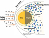 |
Fig. 1 Sketch of the Venusian ionosphere environment and its interaction with solar wind (not to scale). |
2 Theoretical model formulation
Based on observations of the upper ionosphere of Venus (Lundin et al. 2011), we considered two types of positive ions, H+ and O+ (indicated in the text with subscripts H and O, respectively) and negative electrons shown with subscript (e). The ionospheric populations interact with solar wind protons (sp) and electrons (se). The dynamics of these plasmas can be described by the following multi-fluid hydrodynamic equations, according to which each species is governed by continuity and momentum equations. For the hydrogen ions, we have
![Mathematical equation: $\[\frac{\partial n_{\mathrm{H}}}{\partial t}+\frac{\partial}{\partial x}\left(n_{\mathrm{H}} u_{\mathrm{H}}\right)=0,\]$](/articles/aa/full_html/2024/05/aa45773-22/aa45773-22-eq1.png) (1)
(1)
![Mathematical equation: $\[m_{\mathrm{H}} n_{\mathrm{H}}\left(\frac{\partial}{\partial t}+u_{\mathrm{H}} \frac{\partial}{\partial x}\right) u_{\mathrm{H}}+Z_{\mathrm{H}} e n_{\mathrm{H}} \frac{\partial \phi}{\partial x}+\frac{\partial P_{\mathrm{H}}}{\partial x}=0 .\]$](/articles/aa/full_html/2024/05/aa45773-22/aa45773-22-eq2.png) (2)
(2)
For the oxygen ions, we have
![Mathematical equation: $\[\frac{\partial n_{\mathrm{O}}}{\partial t}+\frac{\partial}{\partial x}\left(n_{\mathrm{O}} u_{\mathrm{O}}\right)=0,\]$](/articles/aa/full_html/2024/05/aa45773-22/aa45773-22-eq3.png) (3)
(3)
![Mathematical equation: $\[m_{\mathrm{O}} n_{\mathrm{O}}\left(\frac{\partial}{\partial t}+u_{\mathrm{O}} \frac{\partial}{\partial x}\right) u_{\mathrm{O}}+Z_{\mathrm{O}} e n_{\mathrm{O}} \frac{\partial \phi}{\partial x}+\frac{\partial P_{\mathrm{O}}}{\partial x}=0,\]$](/articles/aa/full_html/2024/05/aa45773-22/aa45773-22-eq4.png) (4)
(4)
and for the electrons, we have
![Mathematical equation: $\[\frac{\partial n_{\mathrm{e}}}{\partial t}+\frac{\partial}{\partial x}\left(n_{\mathrm{e}} u_{\mathrm{e}}\right)=0,\]$](/articles/aa/full_html/2024/05/aa45773-22/aa45773-22-eq5.png) (5)
(5)
![Mathematical equation: $\[m_{\mathrm{e}} n_{\mathrm{e}}\left(\frac{\partial}{\partial t}+u_{\mathrm{e}} \frac{\partial}{\partial x}\right) u_{\mathrm{e}}+Z_{\mathrm{e}} e n_{\mathrm{e}} \frac{\partial \phi}{\partial x}+\frac{\partial P_{\mathrm{e}}}{\partial x}=0.\]$](/articles/aa/full_html/2024/05/aa45773-22/aa45773-22-eq6.png) (6)
(6)
Solar wind protons and electrons are represented by
![Mathematical equation: $\[\frac{\partial n_{\mathrm{sp}}}{\partial t}+\frac{\partial}{\partial x}\left(n_{\mathrm{sp}} u_{\mathrm{sp}}\right)=0,\]$](/articles/aa/full_html/2024/05/aa45773-22/aa45773-22-eq7.png) (7)
(7)
![Mathematical equation: $\[m_{\mathrm{sp}} n_{\mathrm{sp}}\left(\frac{\partial}{\partial t}+u_{\mathrm{sp}} \frac{\partial}{\partial x}\right) u_{\mathrm{sp}}+Z_{\mathrm{sp}} e n_{\mathrm{sp}} \frac{\partial \phi}{\partial x}+\frac{\partial P_{\mathrm{sp}}}{\partial x}=0,\]$](/articles/aa/full_html/2024/05/aa45773-22/aa45773-22-eq8.png) (8)
(8)
![Mathematical equation: $\[\frac{\partial n_{\mathrm{se}}}{\partial t}+\frac{\partial}{\partial x}\left(n_{\mathrm{se}} u_{\mathrm{se}}\right)=0,\]$](/articles/aa/full_html/2024/05/aa45773-22/aa45773-22-eq9.png) (9)
(9)
![Mathematical equation: $\[m_{\mathrm{se}} n_{\mathrm{se}}\left(\frac{\partial}{\partial t}+u_{\mathrm{se}} \frac{\partial}{\partial x}\right) u_{\mathrm{se}}+Z_{\mathrm{se}} e n_{\mathrm{se}} \frac{\partial \phi}{\partial x}+\frac{\partial P_{\mathrm{se}}}{\partial x}=0 .\]$](/articles/aa/full_html/2024/05/aa45773-22/aa45773-22-eq10.png) (10)
(10)
We also used the following plasma neutrality condition
![Mathematical equation: $\[Z_{\mathrm{O}} n_{\mathrm{O}}+Z_{\mathrm{H}} n_{\mathrm{H}}+Z_{\mathrm{e}} n_{\mathrm{e}}+Z_{\mathrm{sp}} n_{\mathrm{sp}}+Z_{\mathrm{se}} n_{\mathrm{se}}=0,\]$](/articles/aa/full_html/2024/05/aa45773-22/aa45773-22-eq11.png) (11)
(11)
We note that the use of the quasi-neutrality condition (Eq. (11)) allows for the Poisson equation to be explicitly avoided, thus keeping all ordinary differential equations in the first order.
The symbols nj, uj, Pj, and ϕ refer to densities, velocities, thermal pressures of the different species, and electric potential, respectively, where j = H, O, e, sp, and se. The system of Eqs. (1)–(11) is closed by the equations of state relating Pj to nj. We used the equation of state of an isothermal ideal gas pressure Pj = kBTjnj, where kB is the Boltzmann constant and Tj is the constant temperature of the different species j of particles with mass mj and charge number Zj. Moreover, mj and Zj are the masses and charge numbers of different species, where ZH,O,sp = −Ze,se = 1. It is also worth mentioning that our study is a local analysis (to fulfil the self-similarity) where the temperature is kept constant, and as we show in Figs. 2–4 that range of the self-similar variable (and the related spatial scale and timescale) is very small compared to Venus’ ionosphere scale.
We needed to solve the system of Eqs. (1)–(11) together. However, solving the nonlinear partial differential equations in the present form is not an easy task to accomplish, even for numerical computations. We hence adopted a self-similar transformation in order to convert the partial differential equations into ordinary differential ones to describe the plasma expansion. By doing this, we characterised the expanding plasma in a co-moving frame with a velocity given by the ion acoustic speed cs = (kBTe/mO)1/2. This method is often applied in studies to understand the various processes in laboratory plasmas (Mora 2003; Djebli 2003; Djebli et al. 2004) space plasmas (El-Labany et al. 2014; Salem et al. 2020; Moslem et al. 2019), creation of surface nano-structures (Moslem & El-Said 2012), laser-plasma interactions (Bennaceur-Doumaz et al. 2015; Shahmansouri et al. 2017), and the dynamics of astrophysical objects (Moslem 2012; Lazar et al. 2012; Elkamash & Kourakis 2016). This approach requires introducing a new variable ξ = x/(cst) in Eqs. (1)–(11), which enables us to convert the above nonlinear partial differential equations into the following nonlinear ordinary differential equations
![Mathematical equation: $\[\left(V_{\mathrm{H}}-\xi\right) \frac{\mathrm{d} N_{\mathrm{H}}}{\mathrm{d} \xi}+N_{\mathrm{H}} \frac{\mathrm{d} V_{\mathrm{H}}}{\mathrm{d} \xi}=0,\]$](/articles/aa/full_html/2024/05/aa45773-22/aa45773-22-eq12.png) (12)
(12)
![Mathematical equation: $\[\left(Q_{\mathrm{H}} \sigma_H \frac{1}{N_{\mathrm{H}}}\right) \frac{\mathrm{d} N_{\mathrm{H}}}{\mathrm{d} \xi}+\left(V_{\mathrm{H}}-\xi\right) \frac{\mathrm{d} V_{\mathrm{H}}}{\mathrm{d} \xi}+Q_{\mathrm{H}} \frac{\mathrm{d} \Phi}{\mathrm{d} \xi}=0,\]$](/articles/aa/full_html/2024/05/aa45773-22/aa45773-22-eq13.png) (13)
(13)
![Mathematical equation: $\[\left(V_{\mathrm{O}}-\xi\right) \frac{\mathrm{d} N_{\mathrm{O}}}{\mathrm{d} \xi}+N_{\mathrm{O}} \frac{\mathrm{d} V_O}{\mathrm{~d} \xi}=0,\]$](/articles/aa/full_html/2024/05/aa45773-22/aa45773-22-eq14.png) (14)
(14)
![Mathematical equation: $\[\left(\sigma_o \frac{1}{N_{\mathrm{O}}}\right) \frac{\mathrm{d} N_{\mathrm{O}}}{\mathrm{d} \xi}+\left(V_{\mathrm{O}}-\xi\right) \frac{\mathrm{d} V_O}{\mathrm{~d} \xi}+\frac{\mathrm{d} \Phi}{\mathrm{d} \xi}=0,\]$](/articles/aa/full_html/2024/05/aa45773-22/aa45773-22-eq15.png) (15)
(15)
![Mathematical equation: $\[\left(V_{\mathrm{e}}-\xi\right) \frac{\mathrm{d} N_{\mathrm{e}}}{\mathrm{d} \xi}+N_{\mathrm{e}} \frac{\mathrm{d} V_{\mathrm{e}}}{\mathrm{d} \xi}=0,\]$](/articles/aa/full_html/2024/05/aa45773-22/aa45773-22-eq16.png) (16)
(16)
![Mathematical equation: $\[\left(Q_{\mathrm{e}} \frac{1}{N_{\mathrm{e}}}\right) \frac{\mathrm{d} N_{\mathrm{e}}}{\mathrm{d} \xi}+\left(V_{\mathrm{e}}-\xi\right) \frac{\mathrm{d} V_{\mathrm{e}}}{\mathrm{d} \xi}-Q_{\mathrm{e}} \frac{\mathrm{d} \Phi}{\mathrm{d} \xi}=0,\]$](/articles/aa/full_html/2024/05/aa45773-22/aa45773-22-eq17.png) (17)
(17)
![Mathematical equation: $\[\left(V_{\mathrm{sp}}-\xi\right) \frac{\mathrm{d} N_{\mathrm{sp}}}{\mathrm{d} \xi}+N_{\mathrm{sp}} \frac{\mathrm{d} V_{\mathrm{sp}}}{\mathrm{d} \xi}=0,\]$](/articles/aa/full_html/2024/05/aa45773-22/aa45773-22-eq18.png) (18)
(18)
![Mathematical equation: $\[\left(Q_{\mathrm{sp}} \sigma_{\mathrm{sp}} \frac{1}{N_{\mathrm{sp}}}\right) \frac{\mathrm{d} N_{\mathrm{sp}}}{\mathrm{d} \xi}+\left(V_{\mathrm{sp}}-\xi\right) \frac{\mathrm{d} V_{\mathrm{sp}}}{\mathrm{d} \xi}+Q_{\mathrm{sp}} \frac{\mathrm{d} \Phi}{\mathrm{d} \xi}=0,\]$](/articles/aa/full_html/2024/05/aa45773-22/aa45773-22-eq19.png) (19)
(19)
![Mathematical equation: $\[\left(V_{\mathrm{se}}-\xi\right) \frac{\mathrm{d} N_{\mathrm{se}}}{\mathrm{d} \xi}+N_{\mathrm{se}} \frac{\mathrm{d} V_{\mathrm{se}}}{\mathrm{d} \xi}=0,\]$](/articles/aa/full_html/2024/05/aa45773-22/aa45773-22-eq20.png) (20)
(20)
![Mathematical equation: $\[\left(Q_{\mathrm{se}} \sigma_{\mathrm{se}} \frac{1}{N_{\mathrm{se}}}\right) \frac{\mathrm{d} N_{\mathrm{se}}}{\mathrm{d} \xi}+\left(V_{\mathrm{se}}-\xi\right) \frac{\mathrm{d} V_{\mathrm{se}}}{\mathrm{d} \xi}-Q_{\mathrm{se}} \frac{\mathrm{d} \Phi}{\mathrm{d} \xi}=0,\]$](/articles/aa/full_html/2024/05/aa45773-22/aa45773-22-eq21.png) (21)
(21)
![Mathematical equation: $\[\alpha \frac{\mathrm{d} N_{\mathrm{H}}}{\mathrm{d} \xi}+\frac{\mathrm{d} N_{\mathrm{O}}}{\mathrm{d} \xi}-\beta \frac{\mathrm{d} N_{\mathrm{e}}}{\mathrm{d} \xi}+\gamma \frac{\mathrm{d} N_{\mathrm{sp}}}{\mathrm{d} \xi}-\delta \frac{\mathrm{d} N_{\mathrm{se}}}{\mathrm{d} \xi}=0 .\]$](/articles/aa/full_html/2024/05/aa45773-22/aa45773-22-eq22.png) (22)
(22)
We note that we used Eq. (11) in a differential form with Eq. (22) so that we dealt with 11 ordinary differential equations.
The normalised quantities are σj = Tj/Te; Qj = mO/mj; α = nH0/nO0; β = ne0/nO0; γ = nsp0/nO0; and δ = nsp0/nO0. The term Nj is the (dimensionless) density that is normalised by the unperturbed density nj0, Vs0 is the initial normalised streaming velocity, and Vs is the dimensionless perturbed velocity normalised by the ion-acoustic speed cs. Finally, Φ is the dimensionless potential which is normalised by kBTe/e, and Pj is the pressure that is normalized by nj0kBTj. Due to the locality of the region studied as a consequence of the normalisation with the ion-acoustic speed, a Cartesian approach was justified (on such small scales, the large-scale divergence of the flow is negligible).
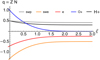 |
Fig. 2 Testing the plasma quasi-neutrality. The hydrogen (black), oxygen (blue), electron (red), solar wind proton (orange), and solar wind electron (grey) charge densities add up to zero. |
3 Results and numerical investigation
3.1 Method
In this section, we numerically investigate the features of the plasma expansion profiles for both oxygen and hydrogen ions. But before that, it is helpful for the sake of reproducibility of the data to give an adequate description of the mathematical method used, the initial conditions, and the motivation behind them. We used the self-similar technique in order to be able to solve the set of hydrodynamic fluid equations that describe the plasma expansion. Although the equations become solvable with the self-similar approach, the space and time are abstracted into a single general dimensionless variable ξ that expresses both the space and time in terms of the physical parameters of our plasma such as acoustic speed cs, plasma Debye length λDe, and the inverse of the plasma frequency 1/ωp. With the aid of the Wolfram Mathematica package, we used the NDSolve command that employs the LSODA (Livermore solver of the ordinary differential equations automatic) approach, the implicit differential algebraic (IDA) equations, and the Hermite interpolation method to numerically solve the system of differential equations Hindmarsh (1983). Therefore, in the following we not only show the solutions as functions of the self-similar variable ξ but also as functions of the physical variable x and t.
3.2 Initial conditions
We were motivated by the data coming from VEX flybys in Lundin et al. (2011) and Knudsen et al. (2016) who reported that O+ ion flow is accelerated to velocities of around 10 km s−1 (escaping velocity) inside the dayside ionopause, while the H+ ion flow is accelerated to velocities that exceed 65 km s−1. The measured composition of the plasma escape differs from the plasma composition in the ionosphere at an ionopause altitude of 300 km for minimum solar wind conditions Fox (2004). We used the typical dawn-dusk ionospheric data for the oxygen, hydrogen, and solar wind proton ions number densities (45–200), (5–20), and (3–20) cm−3, respectively. Also, we used the oxygen, hydrogen and solar wind proton velocity data as (0.5–20), (1–35), and (10–250) km s−1 (Lundin et al. 2011). We got the electron and solar wind electron data from Knudsen et al. (2016): electron density ne = (5–100) cm−3 and electron temperature Te = (6–12) eV, and solar wind electron density nse = (10–200) cm−3 and temperature of Tse = (10–500) eV. In order to apply the normalisation, we introduced the acoustic speed (i.e. the factor with which we have normalized all velocities). We calculated this acoustic speed from cs = ![Mathematical equation: $\[\sqrt{k_{\mathrm{B}} T_{\mathrm{e}} / m_{\mathrm{O}}}\]$](/articles/aa/full_html/2024/05/aa45773-22/aa45773-22-eq23.png) = (5.8–8.3) km s−1. We then calculated the normalised value of the velocity of each species that would be implemented into the numerical code included in the Mathematica package. After normalisation, we obtained the following values: α = nH/nO = (0.05–0.5); β = ne/nO = (0.1–1); γ = nsp/nO = (0.05–0.5); and δ = nse/nO = (0.1–1) for the densities and σO = TO/Te = (0.01–0.1); σH = TH/Te = (0.01–0.1); σsp = Tsp/Te = (1–10); and σse = Tse/Te = (1–10) for the temperatures. For the unperturbed initial velocity, we got υsp[0] = υsp/cs = (1–30) and υse[0] = υse/cs = (1–30). To run the numerical code, we used all the normalised physical parameters above, for example, the values of density, temperature ratio, and initial streaming velocity. We also (according to the observational data) used the initial values, nH[0] = nO[0] = ne[0] = nse[0] = nsp[0] = 1; υH[0] = 5; υO[0] = 1; υe[0] = 10; υsp[0] = 10; υse[0] = 10; and Φ[0] = 0.
= (5.8–8.3) km s−1. We then calculated the normalised value of the velocity of each species that would be implemented into the numerical code included in the Mathematica package. After normalisation, we obtained the following values: α = nH/nO = (0.05–0.5); β = ne/nO = (0.1–1); γ = nsp/nO = (0.05–0.5); and δ = nse/nO = (0.1–1) for the densities and σO = TO/Te = (0.01–0.1); σH = TH/Te = (0.01–0.1); σsp = Tsp/Te = (1–10); and σse = Tse/Te = (1–10) for the temperatures. For the unperturbed initial velocity, we got υsp[0] = υsp/cs = (1–30) and υse[0] = υse/cs = (1–30). To run the numerical code, we used all the normalised physical parameters above, for example, the values of density, temperature ratio, and initial streaming velocity. We also (according to the observational data) used the initial values, nH[0] = nO[0] = ne[0] = nse[0] = nsp[0] = 1; υH[0] = 5; υO[0] = 1; υe[0] = 10; υsp[0] = 10; υse[0] = 10; and Φ[0] = 0.
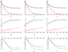 |
Fig. 3 Profiles of the number density (a–c), velocity (d–f), and electric potential (g–i) for both hydrogen (black) and oxygen (red) for two values of the solar wind initial velocity Vsp[0] = Vse[0] = 10 (solid) and 30 (dashed) in the left column, for the temperature ratios σsp = σse = 1 (solid) and 1.5 (dashed) in the middle column, and for the initial solar wind number density ratio γ = 0.5 (solid) and 0.2 (dashed) in the right column. |
3.3 Study of the plasma parameters
We examined the effects of the different parameters of solar wind (initial velocity, temperature, and number density) on the number density, velocity, and the electric potential generated by the plasma expansion at Venus’ ionosphere as a function of the self-similar variable ξ. As shown in Fig. 2, we first tested the quasi-neutrality of the plasma and checked for the validation of the neutrality condition (which is represented in Eq. (22)), which means that at any given moment during the expansion, the sum of all charge densities is zero, as we were dealing with a quasi-neutral plasma. Figure 3 introduces the main findings of the study in the ξ coordinate, while Fig. 4 shows a special case where we returned ξ into x (in a, b, c, d, and e) and t (in f) coordinates.
Next, in Fig. 3 we studied the effect of the solar wind’s proton and electron initial velocities on the number density of the expanding plasma of hydrogen and oxygen in Fig. 3a, the hydrogen and oxygen velocities (Fig. 3d), and on the electric potential generated during the expansion (Fig. 3g). The effect of the solar wind’s proton and electron temperature to electron temperature ratio on the Venusian hydrogen and oxygen number density is shown in Fig. 3b, the impact on the hydrogen and oxygen velocities is shown in Fig. 3e, and the effect on the electric potential generated during the expansion is shown in Fig. 3h. Finally, the effect of the solar wind’s proton-to-oxygen density ratio on the Venusian hydrogen and oxygen number density is shown in Fig. 3c, on the hydrogen and oxygen velocities in Fig. 3f, and on the electric potential generated during the expansion in Fig. 3i. The main result we obtained from this numerical study is that the difference in timescale between the different ion species (Venus plasma and solar wind) plays a crucial role in the interaction between both the solar wind streams and the ionospheric plasma and the behaviour of the plasma expansion. The smaller the difference in the timescale is, the more interaction and the more significant of an effect we get. From the density and velocity figures in Figs. 3 and 4, we noticed that the hydrogen ions are more affected by the streaming properties due to a smaller difference in timescale. The general trend we derived from Fig. 3 is that the depletion in the hydrogen density is less than that in the oxygen density (i.e. the oxygen number density is more sensitive to the variation in the solar wind’s parameters than the hydrogen density) and the expanding hydrogen velocity is higher than the expanding oxygen velocity. This could explain the observational fact that oxygen represents the majority in Venus’ upper ionosphere over hydrogen since the latter acquires a higher velocity due to its lower mass (i.e. less inertia), which enables it to escape Venus’ gravitational field. The electric potential drops to almost 1.2. We translated this value into the un-normalised electric potential in order to calculate the actual value, and we found it to match with the observational electric field drop in the ionosphere of Venus.
In Fig. 3a, one can notice that the depletion in the oxygen density increases when increasing the solar wind velocity. The complete opposite case occurs with hydrogen density as the initial velocity of the solar wind’s protons and electrons increases from 10 to 30 times the ion acoustic speed cs. This could lead to more accumulation of oxygen densities at a higher altitude than where the hydrogen ions reside. In Fig. 3d, we found that both hydrogen and oxygen velocities are slightly affected by the solar wind’s initial streaming velocity (Vsp,se[0]). We also noticed that the hydrogen density shrinks as the solar winds become warmer in Fig. 3b or less dense (as in Fig. 3c) while the oxygen density’s depletion rate becomes enhanced in both of them. In Fig. 3e we examined the effect of the solar wind proton temperature Tsp to electron temperature Te ratio σsp and the effect of the solar wind electron temperature Tse on the electron temperature Te ratio σse and on the velocities of the expanding plasma. We observed that both the hydrogen and oxygen expanding velocities become higher as the solar wind-to-electron temperature ratio gets larger. This is reasonable, as the thermal energy coming from the solar wind can increase the instability of the plasma at Venus and energise their ions as their temperature increases. In Fig. 3f, the velocity of the expanding hydrogen and oxygen increases as the ratio of the solar wind proton to oxygen density gets smaller. Figures 3h and i show that the electric potential drop increases as the solar wind temperature increases (i.e. larger σse and σsp) or becomes less dense (i.e. lower γ).
We show all four density profiles displayed in Fig. 3a also in Figs. 4a and b. For the profile with Vsp[0] = Vse[0] = 10, we also show the time evolution. In Fig. 4, we transformed the dependence on the dimensionless self-similar variable ξ into the dimensional coordinates of x and t. Although we obtained the same behaviour as in Fig. 3, we noticed that the density of the expanding plasma becomes flattened as time passes and the limited x range supports the locality of the analysis. We note that for a fixed time (t = const.), the variables ξ and x are proportional to each other. Particularly, for the normalisation of x/t with cs these variables are identical at time t = τ = 1 s and the distance x = ct × t in kilometre, as can be seen when comparing Fig. 3a or Fig. 3b with Figs. 4a and b.
In Figs. 4c and d, in addition to the difference in hydrogen and oxygen velocity, we observed that the expanding plasma becomes slower and its velocity gets closer to its initial values. This can be explained through an analogy of the expansion of an inflated balloon: After enough time, the expanding gas out of a balloon becomes slower and more stable with the surroundings. Lower densities are specific to locations at greater distances. Lastly, in Fig. 4f we saw a time profile for the oxygen density as a special case, and we noticed that with increasing time at a fixed point at a certain distance from the interaction centre, the number density of the expanding material passing through this point increases. This can be readily understood because for a fixed location x, the similarity variable and the time are inversely proportional to each other, which is straightforwardly explains the principal behaviour of the number density profiles (namely an increase with time) shown in Fig. 4f if they decrease with ξ (as displayed in the first row of Fig. 3).
The hydrogen ions were accelerated to higher values than the oxygen ions. As can be seen in the velocity graphs (Figs. 3d–f, 4c, and d), the oxygen ion velocity profiles have an upper limit almost equal to three times the ion acoustic speed cs. This upper limit is lower than that of the hydrogen velocity, which is more than eight times cs. This gave us a hint as to why the hydrogen composition percentage in the ionosphere of Venus is nine times lower than the oxygen percentage and why the hydrogen velocity is much higher than the escape velocity (10 km s−1) and the oxygen velocity. We could also see that the normalised velocity of the oxygen ions reaches a maximum value of almost 3.2. If this value is converted into real un-normalised velocity by multiplying by the minimum acoustic speed (normalisation factor) ![Mathematical equation: $\[\sqrt{k_{\mathrm{B}} T_{\mathrm{e}} / m_{\mathrm{O}}}\]$](/articles/aa/full_html/2024/05/aa45773-22/aa45773-22-eq24.png) of our plasma regime at Venus ionosphere, we get the real velocity of oxygen VO = 3.2 csO = 15 km s−1, which is comparable to the escaping velocity in Venus’ ionosphere at altitudes of 1000 km. This explains the majority (90%) of oxygen ionic composition at that level of the ionosphere. While for oxygen, the normalised (dimensionless) velocity reaches a value that is much higher than the escaping velocity. Performing the same analysis of “de-normalisation” again but for hydrogen, we obtained the actual velocity of hydrogen in the range of (43–68) km s−1. This range was acquired because of the plasma expansion and ion acceleration, which obviously far exceeds the escaping velocity in Venus’ ionosphere if they are compared with each other. This also matches the observational data obtained from the flybys by VEX, which are cited in Lundin et al. (2011).
of our plasma regime at Venus ionosphere, we get the real velocity of oxygen VO = 3.2 csO = 15 km s−1, which is comparable to the escaping velocity in Venus’ ionosphere at altitudes of 1000 km. This explains the majority (90%) of oxygen ionic composition at that level of the ionosphere. While for oxygen, the normalised (dimensionless) velocity reaches a value that is much higher than the escaping velocity. Performing the same analysis of “de-normalisation” again but for hydrogen, we obtained the actual velocity of hydrogen in the range of (43–68) km s−1. This range was acquired because of the plasma expansion and ion acceleration, which obviously far exceeds the escaping velocity in Venus’ ionosphere if they are compared with each other. This also matches the observational data obtained from the flybys by VEX, which are cited in Lundin et al. (2011).
After showing Fig. 3 and its special cases of Fig. 4, it is worth mentioning that the latter represents a more directly accessible picture of the expansion by displaying the solutions as functions of both x and t instead of ξ. Since ξ = x/(cst), ξ and x are directly proportional for a fixed time t (black lines in Figs. 3a, 4a). Hence, we can replicate such plots as Figs. 3a as (4a and b) but with x instead of ξ. With the same argument, we can also plot density versus time at given (fixed) locations (e.g. in Fig. 4f). As one can see, the behaviour of density versus time is opposite to that of density versus ξ, as expected because ξ and t are inversely proportional.
It is also worth paying attention to the units in Fig. 4, where the distance x is normalised to the length scale λ that we can calculate from λ = csτ and for time τ = 1 s. We can plug in cs = 5.8–8.3 km s−1 from Table 1 into the equation in order to get the value for the plasma length scale as λ = 5.8–8.3 km. To summarise the above discussion, while Fig. 3 displays all results of the parameter study of the dependence on the self-similar transformation variable ξ and is meant to show the variation of the plasma parameters under the influence of the solar wind parameters, Fig. 4 shows these results for selected cases as functions of the physical variables x and t and thereby provides a more directly accessible illustration of the behaviour of the plasma profiles in real (configuration) space.
As a result of studying the plasma expansion of Venus’ ionosphere, one can (with the aid of data from Figs. 3a and d) calculate a rough estimate for the ion escaping flux rates from the ionosphere for both ions H+ and O+ by NH × n0 × υH × cs × 4πR2V and NO × n0 × υO × cs × 4πR2V, respectively. Where NH,O are the normalised number densities of H+ or O+, υH,O are the normalised velocities of H+ or O+, and RV is the radius of the planet. And with the aid of normalisation parameters (i.e. from Table 1 of n0 = 45 cm−3 and cs = 5.8 km s−1), one can obtain values on the order of 5.78 × 1026 particles s−1 for H+ and 3.85 × 1025 particles s−1 for O+. Noticing that the rate of the escaping flux of H+ is higher than that of O+ by an order of 10, this also gives a reason for why the majority of the population in the ionosphere of Venus at altitudes of ~ 1000 km is composed of O+. This is in agreement with the observations and calculations reported in Masunaga et al. (2019); Persson et al. (2020).
The electric potential drop generated from oxygen ions is about 50 times the one generated from hydrogen ions. This could be attributed to the higher atomic number that oxygen has and the higher composition density in the ionosphere particularly at altitudes of 1000 km as mentioned in Lundin et al. (2011). As shown in the electric potential Figs. 3g–i, and 4e, the normalised value of the electric potential generated from oxygen expansion reaches a saturation value of almost −1.2, which we can convert into un-normalised real electric potential value by multiplying by the normalisation variable kBTe/e. We can then calculate the electric field E using the Debye length of our plasma environment E = ϕmax/λDe. Therefore, the real value of the electric potential drop is 13 V and the actual value of the electric field generated within this plasma environment is 7.4 V m−1. To a large extent, this value matches the measured electric potential drop in Venus’ ionosphere as reported in Collinson et al. (2016, 2019).
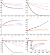 |
Fig. 4 Spatial x (in units of plasma length scale λ = csτ) expansion profiles of (a, b) density, (c, d) velocity, and (e) electric potential for both oxygen (right) and hydrogen (left), respectively, after different time intervals t, including 1 (black), 5 (red-dashed), 10 (blue-dotted), 50 (orange dash-dotted). (f) Time profile (in units of the plasma timescale τ = 1 s) of the oxygen density at different values of distance x: 1 (black), 2 (red-dashed), 3 (blue-dotted), and 4 (orange dash-dotted). Here, the solar wind initial velocity is Vsp[0] = Vse[0] = 10; the ratio of the temperatures is σsp = σse = 1; and for the initial solar wind number density we took the ratio γ = 0.5. The black-dashed lines in (a) to (d) refer to the result at t = 1 for a solar wind initial velocity of Vsp[0] = Vse[0] = 30. |
Plasma parameters.
4 Summary and conclusions
In this study, we performed a nonlinear numerical investigation on the influence of the solar wind streams on the upper ionosphere of Venus and the main features of their interaction. We assumed an appropriate plasma fluid model that simulates the plasma environment at Venus’ ionosphere at altitudes between 200 and 2000 km. Employing a self-similarity approach the model equations were numerically solved and supported with the initial conditions of different plasma variables coming from observational data of VEX and PVO. The results of the study are as follows:
- 1.
The depletion of the hydrogen density due to the interaction with the solar wind is smaller than in the case of oxygen.
- 2.
The hydrogen ions are more influenced by the solar wind proton streaming velocity due to their light mass and the smaller difference in the timescale.
- 3.
The hydrogen ions could be accelerated to velocities that substantially exceed the escaping velocity of Venus’s ionosphere of at altitudes of 1000 km.
- 4.
The oxygen ions are accelerated to velocities comparable to the escaping velocity but are unable to acquire enough acceleration to escape Venus’ ionosphere and subsequently dominantly fill the space in the ionosphere at altitudes of 2000 km.
- 5.
According to our calculations, the electric potential drop of the oxygen ions is found to be within the range of −13 V. This is in agreement with the observational data.
- 6.
Our calculated a rough estimate for the escaping flux rates of ions of O+ and H+ are on the order of 1025 and 1026 particles s−1, respectively.
Future extensions of this study may include the effect of the magnetic field on the plasma expansion profile and it would affect the ionic escaping, as well as the different distribution of the solar wind electrons such as superthermal distribution.
Acknowledgements
The authors acknowledge the sponsorship provided by Alexander von Humboldt Stiftung (Bonn, Germany) in the framework of the Research Group Linkage Programme funded by the respective Federal Ministry. The authors also acknowledge support from the Ruhr-University Bochum, the Katholieke Universiteit Leuven, and Mansoura University. These results were also obtained in the framework of the project SIDC Data Exploitation (ESA Prodex-12).
References
- Barabash, S., Fedorov, A., Sauvaud, J., et al. 2007, Nature, 450, 650 [NASA ADS] [CrossRef] [Google Scholar]
- Bennaceur-Doumaz, D., Bara, D., & Djebli, M. 2015, Laser Particle Beams, 33, 723 [NASA ADS] [CrossRef] [Google Scholar]
- Collinson, G. A., Frahm, R. A., Glocer, A., et al. 2016, Geophys. Res. Lett., 43, 5926 [CrossRef] [Google Scholar]
- Collinson, G., Glocer, A., Xu, S., et al. 2019, Geophys. Res. Lett., 46, 1168 [NASA ADS] [CrossRef] [Google Scholar]
- Djebli, M. 2003, Phys. Plasmas, 10, 4910 [NASA ADS] [CrossRef] [Google Scholar]
- Djebli, M., Annou, R., & Zerguini, T. 2004, Phys. Plasmas, 11, 2267 [NASA ADS] [CrossRef] [Google Scholar]
- Elkamash, I., & Kourakis, I. 2016, Phys. Rev. E, 94, 053202 [NASA ADS] [CrossRef] [Google Scholar]
- El-Labany, S., Moslem, W. M., & Safy, F. 2006, Phys. Plasmas, 13, 082903 [NASA ADS] [CrossRef] [Google Scholar]
- El-Labany, S., El-Razek, A., El-Gamish, G., et al. 2014, Astrophys. Space Sci., 353, 413 [CrossRef] [Google Scholar]
- Fox, J. L. 2004, Adv. Space Res., 33, 132 [NASA ADS] [CrossRef] [Google Scholar]
- Futaana, Y., Stenberg Wieser, G., Barabash, S., & Luhmann, J. G. 2017, Space Sci. Rev., 212, 1453 [NASA ADS] [CrossRef] [Google Scholar]
- Hartle, R., & Grebowsky, J. 1995, Adv. Space Res., 15, 117 [NASA ADS] [CrossRef] [Google Scholar]
- Hindmarsh, A. C. 1983, Sci. Comput., 1, 55 [Google Scholar]
- Intriligator, D. S. 1989, Geophys. Res. Lett., 16, 167 [NASA ADS] [CrossRef] [Google Scholar]
- Knudsen, W. C., Jones, D. E., Peterson, B. G., & Knadler Jr, C. E. 2016, J. Geophys. Res.: Space Phys., 121, 7753 [NASA ADS] [CrossRef] [Google Scholar]
- Lakhina, G., & Singh, S. 2015, Solar Phys., 290, 3033 [NASA ADS] [CrossRef] [Google Scholar]
- Lazar, M., Pierrard, V., Poedts, S., & Schlickeiser, R. 2012, in Multi-scale Dynamical Processes in Space and Astrophysical Plasmas (Springer), 97 [NASA ADS] [CrossRef] [Google Scholar]
- Lundin, R., Barabash, S., Futaana, Y., et al. 2011, Icarus, 215, 751 [NASA ADS] [CrossRef] [Google Scholar]
- Masunaga, K., Futaana, Y., Persson, M., et al. 2019, Icarus, 321, 379 [NASA ADS] [CrossRef] [Google Scholar]
- Meyer-Vernet, N. 2007, Basics of the Solar Wind (Cambridge University Press) [Google Scholar]
- Mihalov, J. D., & Barnes, A. 1982, J. Geophys. Res.: Space Phys., 87, 9045 [NASA ADS] [CrossRef] [Google Scholar]
- Miller, K., & Whitten, R. 1991, Space Sci. Rev., 55, 165 [CrossRef] [Google Scholar]
- Mora, P. 2003, Phys. Rev. Lett., 90, 185002 [NASA ADS] [CrossRef] [Google Scholar]
- Moslem, W. 2012, Astrophys. Space Sci., 342, 351 [NASA ADS] [CrossRef] [Google Scholar]
- Moslem, W., & El-Said, A. 2012, Phys. Plasmas, 19, 123510 [NASA ADS] [CrossRef] [Google Scholar]
- Moslem, W., Salem, S., Sabry, R., et al. 2019, Astrophys. Space Sci., 364, 1 [NASA ADS] [CrossRef] [Google Scholar]
- Nagy, A., Cravens, T., Yee, J.-H., & Stewart, A. 1981, Geophys. Res. Lett., 8, 629 [NASA ADS] [CrossRef] [Google Scholar]
- Persson, M., Futaana, Y., Ramstad, R., et al. 2020, J. Geophys. Res.: Planets, 125, e2019JE006336 [NASA ADS] [CrossRef] [Google Scholar]
- Popel, S., & Morozova, T. 2017, Plasma Phys. Rep., 43, 566 [NASA ADS] [CrossRef] [Google Scholar]
- Salem, S., Moslem, W., Lazar, M., et al. 2020, Adv. Space Res., 65, 129 [NASA ADS] [CrossRef] [Google Scholar]
- Shahmansouri, M., Bemooni, A., & Mamun, A. 2017, J. Plasma Phys., 83, 905830607 [CrossRef] [Google Scholar]
- Sreeraj, T., Singh, S., & Lakhina, G. 2018, Phys. Plasmas, 25, 052902 [NASA ADS] [CrossRef] [Google Scholar]
- Xie, L., Li, L., Zhang, Y., & De Zeeuw, D. L. 2013, Sci. China Earth Sci., 56, 330 [NASA ADS] [CrossRef] [Google Scholar]
- Yadav, V. K. 2021, IETE Tech. Rev., 38, 622 [CrossRef] [Google Scholar]
All Tables
All Figures
|
Fig. 1 Sketch of the Venusian ionosphere environment and its interaction with solar wind (not to scale). |
| In the text | |
|
Fig. 2 Testing the plasma quasi-neutrality. The hydrogen (black), oxygen (blue), electron (red), solar wind proton (orange), and solar wind electron (grey) charge densities add up to zero. |
| In the text | |
|
Fig. 3 Profiles of the number density (a–c), velocity (d–f), and electric potential (g–i) for both hydrogen (black) and oxygen (red) for two values of the solar wind initial velocity Vsp[0] = Vse[0] = 10 (solid) and 30 (dashed) in the left column, for the temperature ratios σsp = σse = 1 (solid) and 1.5 (dashed) in the middle column, and for the initial solar wind number density ratio γ = 0.5 (solid) and 0.2 (dashed) in the right column. |
| In the text | |
|
Fig. 4 Spatial x (in units of plasma length scale λ = csτ) expansion profiles of (a, b) density, (c, d) velocity, and (e) electric potential for both oxygen (right) and hydrogen (left), respectively, after different time intervals t, including 1 (black), 5 (red-dashed), 10 (blue-dotted), 50 (orange dash-dotted). (f) Time profile (in units of the plasma timescale τ = 1 s) of the oxygen density at different values of distance x: 1 (black), 2 (red-dashed), 3 (blue-dotted), and 4 (orange dash-dotted). Here, the solar wind initial velocity is Vsp[0] = Vse[0] = 10; the ratio of the temperatures is σsp = σse = 1; and for the initial solar wind number density we took the ratio γ = 0.5. The black-dashed lines in (a) to (d) refer to the result at t = 1 for a solar wind initial velocity of Vsp[0] = Vse[0] = 30. |
| In the text | |
Current usage metrics show cumulative count of Article Views (full-text article views including HTML views, PDF and ePub downloads, according to the available data) and Abstracts Views on Vision4Press platform.
Data correspond to usage on the plateform after 2015. The current usage metrics is available 48-96 hours after online publication and is updated daily on week days.
Initial download of the metrics may take a while.