| Issue |
A&A
Volume 685, May 2024
|
|
|---|---|---|
| Article Number | A100 | |
| Number of page(s) | 28 | |
| Section | Galactic structure, stellar clusters and populations | |
| DOI | https://doi.org/10.1051/0004-6361/202347380 | |
| Published online | 14 May 2024 | |
The population of young low-mass stars in Trumpler 14⋆,⋆⋆
1
European Southern Observatory, Karl-Schwarzschild-Strasse 2, 85748 Garching bei München, Germany
e-mail: This email address is being protected from spambots. You need JavaScript enabled to view it.
2
Universitäts-Sternwarte München, Ludwig-Maximilians-Universität, Scheinerstr. 1, 81679 Garching bei München, Germany
3
Dipartimento di Fisica e Astronomia (DIFA), Alma Mater Studiorum Università di Bologna, Via Gobetti 93/2, 40129 Bologna, Italy
4
Department of Physics and Astronomy, Rice University, 6100 Main St – MS 108, Houston, TX 77005, USA
5
Centre for Extragalactic Astronomy, Department of Physics, Durham University, South Road, Durham DH1 3LE, UK
6
Institute for Computational Cosmology, Department of Physics, University of Durham, South Road, Durham DH1 3LE, UK
7
Dipartimento di Fisica, Università degli Studi di Milano, Via Celoria 16, 20133 Milano, Italy
8
Universität Heidelberg, Zentrum für Astronomie, Institut für Theoretische Astrophysik, Albert-Ueberle-Straße 2, 69120 Heidelberg, Germany
9
Universität Heidelberg, Interdisziplinäres Zentrum für Wissenschaftliches Rechnen, Im Neuenheimer Feld 205, 69120 Heidelberg, Germany
10
INAF-Istituto di Astrofisica e Planetologia Spaziali, Via del Fosso del Cavaliere 100, 00133 Rome, Italy
11
Université Paris-Saclay, Université Paris Cité, CEA, CNRS, AIM, 91191 Gif-sur-Yvette, France
Received:
6
July
2023
Accepted:
22
September
2023
Abstract
Massive star-forming regions are thought to be the most common birth environments in the Galaxy and the only birth places of very massive stars. Their presence in the stellar cluster alters the conditions within the cluster, impacting at the same time the evolution of other cluster members. In principle, copious amounts of ultraviolet radiation produced by massive stars can remove material from outer parts of the protoplanetary discs around low- and intermediate-mass stars in the process of external photoevaporation, effectively reducing the planet formation capabilities of those discs. Here, we present deep VLT/MUSE observations of low-mass stars in Trumpler 14, one of the most massive, young, and compact clusters in the Carina Nebula Complex. We provide spectral and stellar properties of 717 sources and based on the distribution of stellar ages, derive the cluster age of ∼1 Myr. The majority of the stars in our sample have masses ≤1 M⊙, which makes our spectroscopic catalogue the deepest to date in term of mass and proves that detailed investigations of low-mass stars are possible in the massive but distant regions. Spectroscopic studies of low-mass members of the whole Carina Nebula Complex are missing. Our work marks an important step forward towards filling this gap and sets the stage for follow-up investigations of accretion properties in Trumpler 14.
Key words: stars: formation / stars: low-mass / stars: pre-main sequence / HII regions / open clusters and associations: individual: Trumpler 14 / open clusters and associations: individual: Carina Nebula Complex
Full Tables 1 and D.1 and spectra with fitted templates are available at the CDS via anonymous ftp to cdsarc.cds.unistra.fr (130.79.128.5) or via https://cdsarc.cds.unistra.fr/viz-bin/cat/J/A+A/685/A100
Based on observations collected at the European Southern Observatory under ESO programme 097.C-0137.
© The Authors 2024
 Open Access article, published by EDP Sciences, under the terms of the Creative Commons Attribution License (https://creativecommons.org/licenses/by/4.0), which permits unrestricted use, distribution, and reproduction in any medium, provided the original work is properly cited.
This article is published in open access under the Subscribe to Open model. This email address is being protected from spambots. You need JavaScript enabled to view it. to support open access publication.
1. Introduction
Star formation takes place in both low-mass and massive complexes of molecular clouds. The latter are considered to be more common star-forming environments in the Galaxy (e.g. Miller & Scalo 1978; Lada & Lada 2003; Winter et al. 2018). Those giant regions form hot and massive OB stars, which can significantly affect the formation and evolution of less-massive cluster members. Copious amounts of ionising far (FUV) and extreme ultraviolet (EUV) photons, as well as an enormous volume of ejected mass via outflows or strong stellar winds, can create so-called negative feedback. By injecting large amounts of energy into the surrounding medium, massive stars ionise and disperse the natal molecular cloud producing expanding HII regions (e.g. Freyer et al. 2003; Krumholz et al. 2011; Winter et al. 2018) and remove matter from circumstellar discs that could otherwise be used to form a planetary system (e.g. Adams et al. 2004; Anderson et al. 2013; Facchini et al. 2016; Eisner et al. 2018; Winter & Haworth 2022). On the other hand, expanding shock and ionisation fronts can also compress molecular clouds and in that way trigger the formation of new stars (positive feedback, e.g. Gritschneder et al. 2010; Haworth & Harries 2012). There is a strong evidence that the formation of the Solar System took place in such a large cluster and was heavily influenced by close-by massive stars (e.g. Adams 2010; Pfalzner et al. 2015). It is therefore of great importance to understand how the presence of massive stars in the cluster influences the intrinsic star formation, particularly of low-mass stars, as well as the initial mass function (IMF), star formation efficiency, or the planet formation capacity.
Despite the importance of understanding the global picture of star formation, a substantial part of the investigation was so far focused on nearby (< 300 pc), and therefore low-mass, star-forming regions (Manara et al. 2023). While they are very important in constructing and testing a theory of formation of Sun-like stars, those studies neglect the role of the cluster environment. The closest massive region, the Orion Nebula, although providing excellent first examples of photoevaporating discs (“proplyds”, O’Dell et al. 1993), might not be representative of the most extreme environments where most of the stars in the Galaxy are forming (Smith 2006).
The greatest problem in studying massive star-forming regions is that they are all relatively far away from us (> 1 kpc) and usually suffer from high extinction. These two factors significantly hinder the characterisation (and even detection) of individual members of these complexes, especially those less massive and fainter. Since the stellar content of any cluster is dominated by low-mass stars, lack of those objects can essentially impact results of studies of massive star-forming regions, as well as their interpretation. Moreover, low-mass stars are more vulnerable to the harsh environment than the massive ones (see e.g. Whitworth & Zinnecker 2004; Almendros-Abad et al. 2023). Environmental conditions like high UV radiation also impact the capability of protoplanetary discs around young stars to form planets (e.g. Throop & Bally 2005; Anderson et al. 2013; Facchini et al. 2016; Winter et al. 2018, 2020; Parker 2020; Qiao et al. 2023).
Another observational problem that often accompanies the study of massive regions is a bright and variable emission from the surrounding HII region. Assessment of this emission in most cases cannot be done globally but requires knowledge of the local variation in this emission. This issue is particularly profound when studying emission lines from the young stars, for example tracing accretion, winds, or jets. The stellar spectrum is contaminated with the nebular emission, which can lead to potentially incorrect conclusions. For that reason, fiber-fed spectroscopy is not a good approach to studying star-forming regions. A significantly more efficient way to obtain local and wavelength-dependent sky emission is to employ integral field spectroscopy (IFU) instruments. Current instrumentation offers several IFU spectrographs with medium to high spectral and spatial resolution (e.g. ERIS, MUSE, KMOS at the Very Large Telescopes, or GMOS and NIFS at the Gemini Telescopes, Allington-Smith et al. 2002; McGregor et al. 2003; Bacon et al. 2010; Sharples et al. 2013; Davies et al. 2023). They make it possible to obtain position-dependent spectra of sources of interest and of surrounding background and, with that, to characterise faint objects in distant regions.
The Carina Nebula Complex (CNC) is one of the biggest sites of star formation and one of the most massive HII regions in our Galaxy. It is located in the plane of the Galactic disc at a distance of 2.35 kpc from the Sun (Shull et al. 2021; Göppl & Preibisch 2022), which makes it the closest analog of a typical environment in which stars form. Most if not all the clusters within the CNC are located at similar distances, with a very small distance dispersion of 1−2% (Smith 2006; Cantat-Gaudin et al. 2018; Maíz Apellániz et al. 2020; Göppl & Preibisch 2022; Berlanas et al. 2023). Low interstellar extinction towards the region (e.g. Walborn 1995; Hur et al. 2023) makes it an even more suitable target for observational studies of massive clusters in optical wavelengths. However, it was noticed that the reddening law towards the CNC is anomalous (RV = 4 − 5, e.g. Smith 2002) combined with the variable intracluster extinction (by ∼9 mag Tapia et al. 2003; Rowles & Froebrich 2009; Preibisch et al. 2012). Additionally, the CNC is located close to the Galactic plane, which causes serious problems with contamination of the field stars (in both the foreground and background).
The CNC contains more than 5 × 10⁴ stars (Povich et al. 2019) with a total mass of ∼37 000 M⊙ (Preibisch et al. 2011a) immersed in a massive HII region. While part of the CNC population is spread over a wide area characterised by a low stellar density regime, most of the star formation is confined to a number of star clusters, with Trumpler (Tr) 14, 15, and 16 being the most massive ones. These clusters host the greatest concentrations of O-type stars, which are expected to highly influence the evolution of their low-mass neighbours. There are at least 74 O-type stars in the CNC (Smith 2006; Berlanas et al. 2023), including some of the most massive stars known: prototypical O2 (HD 93129A in Tr 14) and O3 (in Tr 14 and Tr 16) stars, luminous blue variable η Carinae (in Tr 16), and several Wolf-Rayet stars (Walborn 1973; Walborn et al. 2002; Smith 2006).
Current observational campaigns of the CNC are focused mostly on massive or intermediate-mass stars. Photometric studies have included optical, near infrared (NIR), and X-ray observations. More than 100 stars in Tr 14 and Tr 16 were observed by Feinstein et al. (1973) down to G-type stars which allowed the authors to obtain distance values to the clusters close to the most recent ones. DeGioia-Eastwood et al. (2001) investigated over 500 stars in Tr 14 and Tr 16 with optical photometry detecting stars down to ∼1 M⊙. Tapia et al. (2003) presented the optical and NIR photometry of 4150 stars in the CNC with a mass limit of 2 M⊙. Multi-wavelength observations (optical + NIR) were also analysed by Beccari et al. (2015), who built spectral energy distributions (SEDs) of 356 stars, obtained their stellar parameters (down to < 0.4 M⊙), and estimated their mass accretion rates. Optical photometry of stars in Tr 14, Tr 16, and Collinder 232 was analysed by Carraro et al. (2004) down to ∼1 M⊙. Hur et al. (2012) showed visual CCD photometry of the two most massive clusters in CNC and investigated their stellar content together with IMF, with a limit of 1.5 M⊙. They recently extended this catalogue by deep photometry of 135 000 stars down to 0.2 M⊙ in the I band assuming the CNC age of 7 Myr (Hur et al. 2023).
NIR photometry of massive and intermediate-mass stars was published by Ascenso et al. (2007) together with a study of the mass function. Povich et al. (2011) investigated mid-IR excess of ∼1400 young stars in Carina based on Spitzer observations. Extensive, wide-field, and deep NIR photometry of CNC from VISTA and HAWK-I of more than 600 000 sources down to < 0.1 M⊙ was published by Preibisch et al. (2011a,b); Preibisch et al. (2014). Later, Zeidler et al. (2016) investigated their NIR excess. These surveys were often cross-matched with the deep X-ray imaging of the Chandra Carina Complex Project (CCCP, Broos et al. 2011; Townsley et al. 2011), which identified ∼14 000 sources and helped to confirm the youth of low-mass Carina stars. The survey was preceded by a study of Tr 16 with Chandra by Albacete-Colombo et al. (2008) and XMM-Newton observations of early-type stars Antokhin et al. (2008).
Individual, high-mass members of the CNC were classified first photometrically (Walborn 1973, 1995; Massey & Johnson 1993), then spectroscopically (Levato & Malaroda 1982; Morrell et al. 1988; Walborn et al. 2002; Vaidya et al. 2015; Maíz Apellániz et al. 2016; Preibisch et al. 2021; Berlanas et al. 2023). The first spectroscopic properties of massive, intermediate-mass, and solar-like stars in Tr 14 and Tr 16 were obtained in the Gaia-ESO survey by Damiani et al. (2017), who used high-resolution (R ∼ 17 000) observations from the FLAMES/Giraffe spectrometer at the ESO Very Large Telescope (VLT) to characterise more than 1000 stars and to portray the characteristics of those two clusters.
The photometric and spectroscopic works listed above are not a comprehensive list of all studies of the CNC. However, up to date no spectroscopic surveys targeting stars below 1 M⊙ have been conducted in the CNC leaving the most important part of the region uncharacterised. The aim of this work is to fill this gap and provide a spectroscopic catalogue of low-mass stars in one of the main clusters in the CNC, Trumpler 14.
Tr 14 is the most compact and youngest among the three main clusters in the CNC. Its structure has been recognised as consisting of a dense core (r of 0.5′−0.9′ corresponding to 0.3−0.6 pc at the distance of 2.35 kpc) and an extended halo population of possibly slightly older age (4′−7.8′, corresponding to 2.7−5.2 pc Tapia et al. 2003; Ascenso et al. 2007; Kharchenko et al. 2013). Its age is estimated to be ∼1 Myr (Penny et al. 1993; Vazquez et al. 1996; DeGioia-Eastwood et al. 2001; Carraro et al. 2004); 2 Myr younger than Tr 16 (Walborn 1995; Smith & Brooks 2008). It contains ∼20 O-type (Shull et al. 2021; Berlanas et al. 2023) and several dozen B-type stars. As a result, its ultraviolet luminosity is ∼20 times higher than Θ1Ori C in the Orion Nebula (Smith 2006; Smith & Brooks 2008). A high UV field, a high cluster density and mass, a young age, and low reddening towards the cluster make Tr 14 a perfect target for investigating the role of the environment on star formation.
Here, we present the optical photometry and spectroscopy of young, low-mass stars in Tr 14. We define the methodology to detect those faint sources, extract their spectra, assess contamination from the sky emission, and conduct the spectral classification. Subsequently, we describe how the stellar properties are obtained. We conclude our work with a more global outlook on the Tr 14’s properties. This study will be followed up by the detailed characterisation of the accretion properties of the young stars presented here.
2. Data
2.1. Observations and data reduction
Observations were carried out in 2016 with the Multi Unit Spectroscopic Explorer (MUSE), a second generation integral field unit (IFU) instrument on the VLT in Paranal, Chile (Bacon et al. 2010), under the programme ID 097.C-0137 (PI: A. Mc Leod). MUSE covers the wavelength range of 4650−9300 Å with a spectral resolution R ∼ 4000 (sampling of 1.25 Å). Observations were performed without adaptive optics in the Wide Field Mode (WFM) with spatial sampling of 0.2″ and a total field of view of 1′×1′. A wide region around Tr 14, including the core of the cluster and the surrounding molecular cloud, was covered with 22 pointings, with a total integration time per pointing of 39 min. In the ESO archive, there are also “short” exposures available of the total integration time of 15 s, designed for observations of the brightest stars, which we do not use here because we are investigating only the low-mass content of Tr 14. The goal of the project was not only to capture the cluster members, but also to study the kinematics of the gas in the pillar-like structures northeast and southwest of Tr 14. The observations were designed to have a small spatial overlap between individual pointings, and with that smoothly cover the whole area. Each of the pointings was observed three times with a 90° rotation dither pattern to better remove instrument artefacts. Observational logs are presented in Appendix A.
Observations were reduced using the dedicated ESO pipeline v. 2.8.3 (Weilbacher et al. 2020) embedded in the EsoReflex environment (Freudling et al. 2013). The pipeline provides wavelength- and flux-calibrated IFU cubes. The standard stars used for calibration are listed in Appendix A together with the observing conditions. Calibrated exposures were combined into the 3D data cubes, one per field, that were used for the analysis presented in this paper.
2.2. Identification of sources and extraction of spectra
In addition to producing the 3D data cubes, the ESO pipeline allows the user to extract photometric images, among other ones, in the standard Johnson–Cousins bands. We used these images as reference to guide the selection of bona fide sources for the extraction of spectra from the IFU cubes. We used SExtractor (Source–Extractor1, Bertin & Arnouts 1996) to perform the source identification on the photometric images. SExtractor is a free software designed to perform aperture photometry on astronomical images, suited also for crowded regions. It estimates and subtracts the background emission, assuming its smooth variation. We tested the background estimation varying the size of the mesh cell, and found that the size of 16 pixels gives the best performance in terms of recovering large gaseous features on the sky and at the same time not creating artificial ones. The same pixel size is used throughout the aperture photometry and extraction of the spectra. We in fact anticipate here that the latter is done by performing aperture photometry on each individual slice of the MUSE cube at the position of the bona fide sources identified on the I band images.
We first performed the identification of the sources on the I band images, which we used as the reference. We employed a fixed aperture size of 5 pixels in diameter and the background mesh size of 16 pixels. Hence using the SExtractor, we created a catalogue that includes for each source the X and Y position in the MUSE CCD reference frame together with I band aperture magnitudes. Based on the “identification” image, we ran the SExtractor in double image mode on all the photometric images, obtaining magnitudes from other bands, namely R and V. This was possible as all the images have identical dimensions, being all extracted from the same IFU cube. With that we created the initial photometric catalogue of 5428 objects with I band magnitude measurements.
We used the same approach to extract spectra from the MUSE cubes of each source detected in the I band images. Upfront, we sliced MUSE datacubes with MissFITS2 (Marmo & Bertin 2008) into individual images, one per spectral element. Then, we ran SExtractor on each slice and estimated the flux of each source within the same aperture as for the photometric images. The measured fluxes of each spectral element were then combined into a single spectrum for each target. In the same way, we extracted wavelength-dependent flux uncertainties and sky spectra. Both were later used to evaluate the quality of the stellar spectra.
2.2.1. Coordinates correction
We transformed the astrometric coordinates of stars extracted from the MUSE cubes to the coordinate system of the recently released Gaia DR3 catalogue (Gaia Collaboration 2023). We first performed a match between the catalogues with a large separation limit (1−2″), separately for each MUSE pointing. We estimated the median offsets of the right ascension and declination for every pointing and adopted them as coordinate corrections. Absolute corrections ranged between 1.46″ and 5.75″ for the right ascension, and between 0.08″ and 2.98″ for the declination. We list the corrections and show the distributions of the offset for each pointing in Appendix B. We applied the corrections to the coordinates of our stars and list them in Table 1.
Catalogue of low-mass stars in Trumpler 14 analysed with MUSE observations.
Consecutively, we matched our catalogue with corrected coordinates once again with Gaia (Gaia Collaboration 2016, 2023). We find 1902 counterparts within the separation of 0.5″. In Appendix B we show the distribution of separations between Gaia and MUSE and argue for the selection of the separation limit. Based on this distribution, we also find that the accuracy of astrometry of our stars is of ∼0.1″.
2.2.2. Identification of spurious sources
Before analysing the sample we removed from the catalogue spurious sources that may be due to a low signal-to-noise ratio (S/N), confusion near the very bright stars, and contamination from the structures in the nebular emission.
Due to different atmospheric conditions the sensitivity of different pointings is uneven. Additionally, some images contain bright stars whose luminosity dominates the images making the detection of the faint sources in their vicinity challenging. We first used flags issued by SExtractor on photometric measurements to exclude potentially incorrect magnitudes. Those flags marked cases when a neighbouring source likely biased the estimation, when the light from the object had been deblended, when the position of the object was too close to the edge of the image, when one or more pixels were saturated, or when the photometry process was corrupted3. With this approach, we removed 21% of the sources from the catalogue. We additionally only accepted stars with the photometric uncertainty in the I band of less than 0.1 mag. We removed photometric measurements not fulfilling those criteria in other bands. This procedure leaves 3082 sources in our catalogue.
The CNC is an HII region, remarkably bright in some atomic lines (Hα, Hβ, OI, HeI, etc.). In particular, small, compact gas concentrations can mimic light from the stars, having a stellar-like point spread function (PSF). We performed a visual inspection of the I band images, comparing them to the other broadband MUSE images, as well as to the HAWK-I H-band image (Preibisch et al. 2011a,b), identifying all possible “spurious” detections that were not present in other images, flagging them accordingly, and removing from the catalogue.
We paid particular attention to the images affected by the presence of nearby saturated stars. Their light was spread on the pixels around their PSF on the CCD detector. This artificially changed the local background, making the measurement of the stellar flux falling on those regions unreliable. Additionally, we identified elongated spikes near those bright stars, due to the diffraction pattern of the secondary mirror support. Combined, those effects significantly hinder the analysis of fainter stars in the closest neighbourhood of the bright ones. Based on a visual inspection, we identified stars where the light was not separated spatially on I band MUSE images from the bright stars, flagged them as “illuminated”, and removed them from the final photometry catalogue, leaving 2727 stars.
2.2.3. Detections in overlapping pointings
The edges of some neighbouring pointings overlapped, causing double detection of the same stars in our photometry catalogue. After correcting the coordinates, we defined a threshold separation of 0.5″ within which we looked for stars present in two (or more) pointings. We found 55 pairs of doubly observed targets. We excluded from the catalogue those sources that had a worse S/N for the spectrum around 7500 Å. We show comparisons of the spectra between two detections in Appendix C.
2.2.4. Background emission
All the images of the CNC, as an HII region, suffer from bright and highly variable background emission. The presence of a strong background with flux variations of the order of one stellar PSF makes the estimation of the local background in the vicinity of the stars very uncertain. Hence, the aperture photometry from which the stellar spectra are built can be very imprecise and unreliable. During the stellar flux extraction (Sect. 2.2), background emission was estimated by SExtractor assuming it varies smoothly across the field. To make sure that the photometry was robust, we estimated the local background variation for each star in our catalogue based on the standard deviation (STD) of the background estimates for stars within a radius of 20″. We adopted a threshold of 3σ, where σ is the STD, and removed all photometric measurements where the stellar flux was below this threshold. In Appendix D we discuss the applied definition in depth. The final number of stars with well defined and reliable I band magnitudes is 804 (Fig. 1).
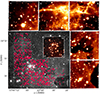 |
Fig. 1. Trumpler 14 cluster studied in this work. Grey sky image from HAWK-I H-band observations (Preibisch et al. 2011a,b) shows the whole region, with the light grey grid of MUSE pointings and stars studied in this work marked as red circles. The five panels above and on the right show selected MUSE I band images. The panel inside consists of a mosaic of four MUSE pointing of the Tr 14 centre. Their numbers are indicated in the panels. Positions of the stars on MUSE images are marked with empty grey circles. The bar on the lower right corner of the HAWK-I image indicates the projected distance of 0.5 pc at the assumed distance of 2.35 kpc towards Tr 14 (Göppl & Preibisch 2022). |
2.2.5. Magnitude correction
To check the flux calibration we compared the MUSE photometry with the optical photometry from the Wide Field Imager (WFI) at the MPG/ESO 2.2 m telescope published by Beccari et al. (2015). The catalogues were matched adopting a 0.5″ maximum separation radius between the stars from the two catalogues. We find 613 common stars in the two catalogues. We performed the comparison of the magnitudes of each field and band separately. For the I band the corrections vary between 0.16 and 1.28 mag depending on the MUSE pointing, with a mean value of 0.55 mag. This is mainly due to the fact that each MUSE field was observed in very different weather conditions. All corrections are provided in Appendix E. We discarded B band magnitudes for being highly uncertain for our faint stars. We provide in the Table 1 the photometry of the sources extracted from the MUSE images with the magnitudes corrected to match the WFI ones.
As a next step, we investigated the distribution of the magnitudes. We show the observed luminosity function for the I, R, and V bands from MUSE observations in Appendix E. The distribution of I band magnitudes peaks at ∼18 mag and falls to ∼21 mag. If we adopt the cluster age of 1 Myr (Smith & Brooks 2008), the distance to the cluster of 2.35 kpc (Göppl & Preibisch 2022), and an extinction of 2.3 mag (see Sect. 3), those magnitudes will correspond to the stellar masses of ∼0.8 and ∼0.14 M⊙ according to the theoretical evolutionary models of Baraffe et al. (2015). Even though we did not correct the luminosity function for completeness, those rough mass estimates show the depth of our catalogue.
2.2.6. Cross-match with other photometry catalogues
To complete our catalogue with information from other wavelength ranges, in addition to the Gaia DR3 and WFI, we cross-matched the MUSE catalogue with VISTA (Preibisch et al. 2014), HAWK-I (Preibisch et al. 2011a,b), Spitzer (Povich et al. 2011), and Chandra (Preibisch et al. 2011b; Townsley et al. 2011) observations. For consistency, we defined the same maximum separation of 0.5″ for all the catalogues. In Appendix B we explain the use of this separation limit. We find 658, 766, 26, and 309 stars in common between MUSE and VISTA, HAWK-I, Spitzer, and Chandra, respectively. We present in Table 1 the example of the catalogue, together with flags indicating the presence of the counterpart in any other catalogue. The full content of the catalogue is available at the CDS.
We emphasise that we adopted a very conservative approach and applied severe photometric quality thresholds and checks to select only bona fide stars with high-quality spectra. In doing so we are aware that a number of real stars that did not pass our photometric quality criteria might have been removed from the final catalogue. In fact, a large number of these stars do have a counterpart in one or more of the catalogues used to complement the MUSE photometry. Among the discarded sources are 841 Gaia, 212 WFI, 913 VISTA, 1809 HAWK-I, 2 Spitzer, and 120 Chandra counterparts. We are aware that within this limitation our catalogue is not complete in terms of cluster members. We report the list of probable members with uncertain photometry due to the background contamination in Table D.1 and assess the completeness in the next section.
2.3. Completeness of the catalog
The goal of this work is to have a high-quality spectroscopic sample of low-mass members of Tr 14. In order to achieve this goal we applied a number of quality cuts to the photometric catalogue (Sect. 2.2.4), which can affect the interpretation of our results.
To better understand the limitations of our work, we estimate the completeness by comparison to the photometric catalogue from HAWK-I (Preibisch et al. 2011a,b). Figure 2 shows the distribution of J-band magnitudes observed by HAWK-I in the exact same region as covered by our MUSE pointings (dark berry-coloured histogram). The stars in common between the two catalogues are shown in violet. With the grey line we show the ratio between the stars retrieved in our catalogue and the number of stars observed by HAWK-I per magnitude bin of 0.5 mag. The ratio gives us a rough estimate of the completeness of our catalogue. The upper panel shows only those stars for which the three sigma level of background variation did not exceed the I band flux measured with MUSE. Their J band magnitudes range from 12.5 to 19.0 mag, corresponding at the low-mass end to 0.065 M⊙ at 1 Myr (Baraffe et al. 2015). Assuming that the HAWK-I catalogue is complete down to ∼21 mag in J-band (Preibisch et al. 2011a), we can adopt this ratio as a rough estimate of the completeness of our catalogue. Based on this assumption, we reach 50% level of completeness at ∼15.5 mag, corresponding to 0.8 M⊙ at 1 Myr. The 30% completeness level is achieved at ∼16.5 mag, corresponding to ∼0.4 M⊙ at 1 Myr. As we indeed see later in Sects. 3.2 or 4.2, our deep observations allow us to detect and characterise very low-mass stars in Tr 14. However, due to our conservative approach to the background emission (Sect. 2.2.4), the final sample is highly incomplete at the low end of the mass spectrum.
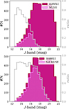 |
Fig. 2. Distribution of J-band magnitudes from HAWK-I in the MUSE field (Preibisch et al. 2011a,b). The dark berry-coloured histogram shows all HAWK-I measurements taken in the same area that was covered by MUSE. The violet distribution presents point source detections from Sect. 2.2.6, (upper panel) and in combination with the one excluded due to the high background variation and foreground stars (lower panel). In both panels, the grey line shows the completeness of our catalogue, defined as a ratio of the number of stars in a given magnitude bin (0.5 mag wide) in our catalogue and in the HAWK-I catalogue. |
In the lower panel of Fig. 2 we include the “full MUSE” sample, consisting of the one with robust I band MUSE photometry and the one discarded due to the highly variable background emission. Here, flagged or uncertain MUSE photometry sources (Sect. 2.2.2) were not included. We see immediately that with our approach we removed mostly faint, low-mass objects. The “full” catalogue extends to the ∼21 J band magnitude (0.018 M⊙ at 1 Myr adopting the evolutionary models of Baraffe et al. 2015) and reaches a 50% level of completeness at ∼18.5 mag, corresponding to 0.085 M⊙ at 1 Myr. The 30% completeness level is achieved at ∼19 mag (0.065 M⊙).
The significant difference between the two distributions (the “MUSE” sample with robust I band photometry and the “full MUSE” sample affected by the background emission) shows the possible impact of the adopted procedure on the final results and the estimated global properties of Tr 14. Since the deep NIR photometric observations can contain a significant fraction of contamination from background sources, especially at the faint end (see the discussion in Sect. 3.3 in Preibisch et al. 2011a and in Sect. 2.3 in Preibisch et al. 2011b), we do not correct our analysis for the incompleteness. We assume that our study is complete at the level of 50% for stars more massive than 0.8 M⊙ and at the level of 30% for stars more massive than 0.4 M⊙.
3. Stellar population
3.1. Identification of foreground stars
To exclude possible contamination from foreground and background stars we used accurate Gaia astrometry for our sources. We first performed a number of quality checks on the matched objects. We first excluded all stars that have a goodness of fit parameter, RUWE > 1.4 (Lindegren 2018), astrometric_gof_al > 5 (Lindegren et al. 2021), a parallax over error lower than 5, and uncertainty of the proper motion above 20%. We flagged them as objects with poor Gaia astrometry, gaia_flag = “poor”. We find 175 good objects out of the 794 Gaia counterparts. None of them is flagged as a non-single star or a duplicated object, reassuring us about the good quality of the astrometry. All of them have a 5- or 6-parameter solution. We selected foreground and background stars based on parallaxes corrected for bias, as described in Lindegren et al. (2021). This correction is possible only for stars with a G band magnitude between 5 and 21, and for the effective wavenumber (for the 5-parameter solution) or the pseudocolour (for the 6-parameter solution) between 1.24 and 1.72 μm−1. Wavenumbers were calculated using calibrated BP/RP spectra, while the pseudocolour is the approximate colour of the source based on its astrometric solution, utilising the chromaticity of the instrument.
We illustrate the distribution of the corrected parallaxes of stars with good Gaia astrometry in Fig. 3. The Gaussian profile fit to the distribution is centred at ϖ = 0.43 mas and has a width of σ = 0.04 mas. The centroid parallax corresponds to the distance of 2.35 kpc, in very good agreement with the findings of Göppl & Preibisch (2022). We followed their procedure to identify foreground and background stars. We defined the background stars as those for which the 3σ extend of the parallax value (i.e. the parallax value plus its error) is smaller than the ϖmin (ϖ + 3σϖ < ϖmin), and the foreground stars as those with a 3σ extent (i.e. the parallax value minus its error) higher than ϖmax (ϖ − 3σϖ > ϖmax). We adopted ϖmin and ϖmax values corresponding to the range of parallaxes defined by the width of the Gaussian distribution (0.43 ± 0.04 mas), further corresponding to the distance range of (2.61 kpc, 2.13 kpc). Out of 175 good Gaia counterparts we identify no background stars and 24 foreground stars. However, if we take into account all possible Gaia matches with corrected and positive parallaxes and possibly high astrometry uncertainties (784 stars), then for the same parallax ranges we find 35 possible foreground stars and 10 possible background stars. We removed from our catalogue 24 foreground stars with robust astrometry and flagged 21 remaining stars as possibly contaminated (foreground or background) stars (possible_frg_bkg). In summary, we find 794 Gaia counterparts, including 175 with good astrometry; 24 of them are foreground stars. In the end, our catalogue contains 780 sources.
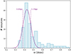 |
Fig. 3. Distribution of corrected parallaxes (light blue histograms) with a fitted normal distribution (purple line). Dash-dotted lines mark the 1σ width of the fitted distribution and applied ranges for excluding foreground and background stars. |
3.2. Colour–magnitude diagram
We first present the colour-magnitude diagrams (CMDs) based on corrected MUSE photometry. Figure 4 shows two CMDs based on (V − I) and (R − I) colours from MUSE, exclusively, and one based on the I band magnitude from MUSE and J-band magnitudes from HAWK-I or VISTA. We also plot PARSEC v1.2S4 theoretical isochrones with solid black lines (Bressan et al. 2012; Chen et al. 2014) reddened by AV = 2.6 mag, best matching our observations (see also Sect. 3.4), using an extinction law of Cardelli et al. (1989) and RV = 4.4 (Hur et al. 2012). We applied a distance modulus of 11.86 mag, equivalent of the distance to Tr 14 (Göppl & Preibisch 2022). We show tracks for 0.3, 0.7, 1, and 3 M⊙ stars with dotted lines. Our observational CMDs already demonstrate that, despite very conservative quality control, our MUSE data allows us to sample stars in Tr 14 with robust I band photometry down to ∼0.3 M⊙. We note, however, that due to the decrease in the S/N at shorter wavelengths, the number of robust R and V band magnitudes is smaller than in the I band, and at the same time the number of very low-mass stars detected in those bands is reduced.
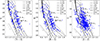 |
Fig. 4. Colour–magnitude diagrams from MUSE broadband filters images in V and I (right panel), R and I magnitudes (middle panel), and I and J magnitudes (left panel). J band magnitudes are from VISTA and HAWK-I instruments. Shown are only data points with I band magnitudes above 3σ. Solid lines show PARSEC isochrones from 0.2 to 20 Myr and ZAMS, dotted lines show isomasses of 0.3, 0.7, 1, and 3 M⊙, as labeled (Bressan et al. 2012). Isochrones were reddened by the average extinction AV = 2.6 mag measured from MUSE spectra (see Sect. 3.4). Additionally, we plot the ZAMS reddened by AV = 1.4 mag with grey lines. |
Ascenso et al. (2007) used high-resolution near-IR data to study the core of Trumpler 14. Based on their photometry they found a global visual extinction towards Tr 14 of AV = 2.6 ± 0.3 mag and a sparse foreground population with an AV of 1.4 mag. In addition to the isochrones reddened by the visual extinction matching our observations, we also show in Fig. 4 the location of the zero age main sequence (ZAMS, solid grey line) reddened by the visual extinction of a sparse population (1.4 mag). The authors suggested that this population of older stars comes from the young clusters nearby. In our CMDs we see an indication of two separate populations, one concentrated around the 1 Myr isochrone, and the other following ZAMS. We note similar two-population CMDs of more massive stars in the work of Carraro et al. (2004, see their Fig. 5). We examine this feature with spectral classification in the following sections.
3.3. Spectral classification
The goal of this paper is to characterise the low-mass members of Trumpler 14 and provide a catalogue of their stellar parameters. As shown in Fig. 4, our dataset samples a wide range of stellar masses and colours, and thus spectral types. Hence, we split the procedure of spectral classification into two cases and give a detailed description in forthcoming sections. We note that our procedure is comparable to the one adopted by Fang et al. (2021) in the study of the Trapezium cluster.
We based the spectral classification on Class III templates observed with the VLT/X-shooter and published by Manara et al. (2013, 2017). The list of templates is provided in Appendix F. Those sources were previously studied in the literature and their spectral types are well known. We note here that they all have a negligible extinction, AV < 0.3 mag. We refer to the Class III templates as “templates” later in the text. We degraded the templates spectra (with a natal resolution of R ∼ 7500 − 18 200) to the MUSE resolution, convolving them with a Gaussian kernel, and then re-sampled them on the spectral range both instruments have in common (∼5500−9350 Å). The comparison between the spectra was done in the aforementioned range after normalising to the flux at 7500 Å, f750.
3.3.1. M-type stars
The spectra of M-type stars have a characteristic shape in the optical range due to the presence of the TiO and VO absorption bands. The depth of those features changes with the spectral sub-type and increases with later stellar types.
In this work, only spectra that have sufficient S/Ns (S/N > 10) were used and classified. From the whole sample of spectra we pre-selected those that might be of M-type based on spectral indices from Riddick et al. (2007), Jeffries et al. (2007), and Oliveira et al. (2003, TiO feature at 7140 Å) and Herczeg & Hillenbrand (2014, TiO 7140, 7700, 8465 Å). We require that at least half of the indices suggest an M-type spectrum. We removed from the spectra prominent emission and absorption lines to prevent confusion in the fitting to the templates. The spectral classification was performed together with the estimation of the visual extinction, AV, and veiling at 7500 Å, r750. We veiled and reddened templates using the Cardelli extinction law (Cardelli et al. 1989) and pre-defined grids of AV and r750 values. The extinction was sampled with a step of 0.1 mag between 0.0 and 7.0 mag, while the veiling was assumed to change between 0.0 and 1.9, with a step of 0.02. The average extinction towards Tr 14 was found to be 2.6 ± 0.3 mag (Ascenso et al. 2007), thus we do not expect a huge variation in AV for cluster members. The adopted sampling of the extinction and veiling is smaller than the typical uncertainty of these parameters assessed later.
We minimised the value of a reduced χ2-like metric, defined as
 (1)
(1)
to find the best combination of spectral type, AV, and r750. O is the observed spectrum, T is the fitted template, err defines the extracted uncertainty of the observed spectrum per spectral bin, i, and N is the number of degrees of freedom (the number of all spectral bins subtracted by three free parameters). Figure 5 shows an example of the result from the fitting procedure, whereas in Appendix G we show the corresponding  maps. We notice that the worst fits usually have marginal values of AV and r750. In total, we classified 269 M-type stars.
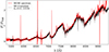 |
Fig. 5. Example of a MUSE spectrum (solid red line) of an M-type star and the matching spectral template (dashed black line). Both spectra are normalised at 7500 Å. |
To assess the uncertainty of the estimated parameters, we ran the fitting again, keeping each time one of the parameters fixed at the best value. We drew the 1-σ curves on the  maps between each two parameters. Examples are shown in Fig. G.1. The maximum and minimum values within 1σ from the best fit of two parameters are indicated by the extreme points of the 1-σ curve. With this procedure we get two pairs of uncertainties for each parameter. We combined them, taking the minimum. The lower and upper uncertainties are reported together with the best-fit values in the Table 1. The uncertainties of the spectral types obtained in this way are on average 2−3 sub-classes, also confirmed by the visual goodness of the fit to the spectra. We note that due to the uneven sampling of spectral types, the
  maps do not represent the true
  . We also emphasise that our method of error assessment introduces a bias towards the values close to the borders of the adopted ranges and causes underestimation of the uncertainty on that side. Therefore, uncertainties for parameter values close to the border should be treated with caution.
3.3.2. K and late G-type stars
The prominent TiO and VO bands in the spectra of M-type stars fade away in mid-K-type stars, while the overall shape of the spectrum flattens. We identify hotter stars in our sample based on the equivalent widths (EWs) of selected absorption lines; we list them in Table G.1. We first calibrated the change in the EWs as a function of spectral type using the Class III templates (Sect. 3.3), assuming a linear correlation. For each line we adopted a single value of the uncertainty of our calibration based on the fit’s uncertainty. Additionally, for late K-type stars we used the spectral index TiO (7140 Å) identified by Oliveira et al. (2003) and Jeffries et al. (2007) and added it to a pool of previous estimates. The final spectral type was assigned as a weighted mean of types from single EWs and indices. Similarly, the uncertainty of the spectral type is a weighted mean of the uncertainties assigned to all of the indices. A single index error is the root of the sum of the squared uncertainties on individual EW measurements and EW calibrations. The resulting values are listed in Table 1.
Once the spectral type was assigned, we performed an estimation of the extinction and veiling following the same approach used to classify the M-type stars (see Sect. 3.3.1). We fitted to observed spectra the templates closest to the estimated spectral types varying AV and r750. The best values are those for which the value of pseudo- ,
,  is minimal. The uncertainties of AV and r750 are estimated based on
  maps, similar to the procedure described in Sect. 3.3.1. An example of the MUSE spectrum of a K-type star with the matched template is shown in Fig. 6. We find 14 early M-, 339 K-, and 95 late G-type stars.
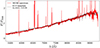 |
Fig. 6. Example of the MUSE spectrum (solid red line) of the K-type star and matching spectral template (dashed black line). Both spectra are normalised at 7500 Å. |
We note that the non-homogeneous sampling of the templates can cause an error on the estimates of stellar parameters that is hard to estimate properly (see the examples of  maps in Appendix G). That applies not only to the spectral types, but also to extinction and veiling. However, for the lowest-mass stars in our sample, the low S/N dominates over any other source of uncertainty. For this reason, we did not interpolate between spectral types of templates to create a homogeneous grid. K- and G-type stars have on average smaller uncertainties in the spectral classification than M-type stars, since for these stellar types the estimate is based on absorption lines and is independent of the density of the grid sampling. A possible source of the large error is the assumption of a linear correlation between the spectral types and EWs. Those relations are usually quadratic (e.g. CaI; Herczeg & Hillenbrand 2014) or higher-order polynomial (e.g. Oliveira et al. 2003; Riddick et al. 2007). Overall, our estimations of spectral type are accurate within 2−3 sub-classes.
3.4. Extinction-corrected colour-magnitude diagrams
As described in Sect. 3.2, the MUSE data presented here allowed us to sample the stellar population in Tr 14 down to very low-mass stars. The observed CMDs shown in Fig. 4 indicate the presence of two populations. Here, after the accurate determination of the stellar parameters using the MUSE spectra (see previous section), we reevaluated this using the extinction values derived for each individual star.
Based on measurements towards individual stars, we estimated the visual extinction towards the Tr 14. The medium value of AV is 2.60 mag. In Fig. 7 we show the distribution of visual extinctions estimated in the previous sections. The distribution has a Gaussian-like shape, and the fitted profile raises a centroid of 2.49 mag, consistent with the findings of Ascenso et al. (2007) and slightly lower than the value reported by Beccari et al. (2015). Our distribution of AV is quite broad, with a Gaussian width of 1.04 mag. On average, the uncertainties of individual AV estimates are ∼0.5 mag. We conclude that our measurements are in line with the literature values, within the uncertainties.
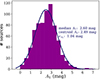 |
Fig. 7. Distribution of AV estimated for Tr 14 stars. Additionally, we fitted the Gaussian function to estimate the centroid of the distribution. The centroid, the width of the distribution, and the median value in our sample are indicated in the upper right part of the figure. |
We used the estimated AV to correct the observed magnitudes. We show de-reddened CMDs in Fig. 8 together with the isochrones from the PARSEC v1.2S models (Bressan et al. 2012). The previously seen two populations are no longer apparent when the new extinction correction is applied, as is expected for differently obscured populations (Ascenso et al. 2007). This reassures us about the correctness of our procedure. The large scatter of points remains; we discuss possible reasons for that in the following sections.
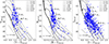 |
Fig. 8. Colour–magnitude diagrams from MUSE broadband filters images in V and I (left panel), R and I magnitudes (middle panel), and I and J magnitudes (right panel) corrected for individual extinction. J-band magnitudes are from the VISTA and HAWK-I observations. Reddening vectors in the lower left corners show reddening by a median value of AV estimated for Tr 14. Solid lines show isochrones from 0.2 to 20 Myr (and ZAMS); dotted lines show isomasses of 0.3, 0.7, 1, and 3 M⊙, as labeled (Bressan et al. 2012). |
4. Physical parameters of the stars
4.1. Effective temperature and stellar luminosity
We derived the effective temperatures (Teff) of our stars based on their spectral types. For M-type stars we used the SpT–Teff scale from Luhman et al. (2003) and for earlier types we applied the scaling from Kenyon & Hartmann (1995) and interpolated linearly between the sub-classes. Newer scales, like for example from Herczeg & Hillenbrand (2014), agree well for low-temperature stars (types later than K5). The scale adopted here deviates for the hotter stars up to 380 K in the case of K0 stars in comparison to Herczeg & Hillenbrand (2014).
It has been shown in the literature that the J-band photometry is most suitable for deriving the bolometric correction for young stars. The spectral energy distribution in these objects can be strongly affected by the presence of NIR excess due to the ongoing mass accretion from a protoplanetary disc or intrinsic differential extinction. Such effects cannot be fully avoided but are minimised using the J-band filter (e.g. Kenyon & Hartmann 1995; Luhman 1999). Our bolometric luminosities were hence calculated using the J-band photometry from VISTA (Preibisch et al. 2014) and HAWK-I (Preibisch et al. 2011a,b). Whenever magnitudes from both catalogues are available for a given star, we chose the one with a smaller uncertainty. We first calculated the bolometric magnitude (Mbol) de-reddening the observed magnitudes by the individual visual extinction determined from our spectral classification (Sect. 3.3) and estimating its value in the J band using the extinction law from Cardelli et al. (1989), subtracting the distance modulus and adding the bolometric correction with colours, as indicated by the equation:
 (2)
(2)
Values of the corrections and colours were taken from Kenyon & Hartmann (1995). Finally, to obtain the bolometric luminosity in L⊙, we subtracted from the previously estimated Mbol the solar bolometric magnitude, Mbol, ⊙ = 4.74 (Cox 2000):
 (3)
(3)
The Lbol values thus calculated are listed in Table 1. Only ∼1% of spectroscopically classified stars in our catalogue were not matched with any source from the NIR catalogues and therefore do not have estimated stellar parameters. This might be due to the fact that the NIR catalogues are not 100% complete.
The uncertainty of the stellar luminosity in our estimations is mostly driven by two factors: the uncertainty of the J band photometry adopted from the VISTA and HAWK-I catalogues, and the uncertainty of the extinction measured by us while performing the spectral classification of each star (Sect. 3.3). The latter has a significantly greater impact: the typical uncertainty of the J band magnitudes used in this work is ∼0.03−0.05 mag, while the average AV error is ∼0.5 mag, corresponding to ΔAJ ∼ 0.16 mag.
4.2. HR diagram and stellar parameters
In Fig. 9 we show the bolometric luminosity as a function of the effective temperature. The stars detected with MUSE are shown with filled circles. The open squares represent the median luminosities for each spectral type. We show on the HR diagram the PARSEC v1.2S theoretical isochrones (Bressan et al. 2012). We assigned the stellar masses and ages by performing linear interpolation between the tracks and the isochrones. The resulting values are listed in Table 1. For stars more luminous than predicted by the lowest-age isochrone we assigned the boundary value of 0.1 Myr as a stellar age.
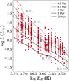 |
Fig. 9. HR diagram for low-mass stars of Tr 14. Filled circles show data points. Empty squares are the median values of the bolometric luminosity for each spectral subclass, with error bars indicating 1-σ percentiles. Theoretical tracks from Bressan et al. (2012) are shown as solid black lines. Dotted grey lines show tracks for 0.3, 0.7, 1, and 3 M⊙ stars. |
The HR diagram (Fig. 9) shows the presence of a large spread of luminosities for sources with the same spectral type. Depending on the spectral type, the spread ranges from 0.5 to 2.0 dex. Possible explanations of this behaviour are two-fold: observational and physical. Observational reasons for the spread cover uncertainties in estimations of stellar luminosity and/or the effective temperature, as well as contamination from foreground sources. As we discussed in Sect. 4.1, the main source of luminosity uncertainty is the extinction, closely linked to the uncertainty of the spectral type (and thus Teff) and veiling. On average, the luminosity values are uncertain by ∼0.3 dex, temperatures by 300 K, and veiling by 0.1−0.3. Given the large distance to Tr 14 (2.35 ± 0.05 kpc, Göppl & Preibisch 2022), we expect a significant contamination by foreground stars. In Sect. 3.1 we therefore used the Gaia DR3 catalogue to minimise this effect and remove objects in the foreground of the CNC. However, the limited number of good astrometric measurements prevents us from identifying all non-cluster members. It is therefore not trivial to estimate the contribution of foreground contamination to our results. This effect, combined with uncertainties in our measurements, can explain a large part of the observed luminosity spread in our HR diagram.
The physical sources of the luminosity spread include intrinsic age spread, variability, binarity, dispersion in distance, and accretion history. Episodic but vigorous accretion of low-mass objects in the very early stages of their formation (Class 0 – Class I) can leave its imprint on their evolution for the next few Myr (Baraffe et al. 2009). If most of the accreting kinetic energy is radiated away, the structure of the star will be more compact (i.e. the stellar radius will be smaller) than that of a non-accreting star of the same age and mass. Short, intense, and numerous accretion episodes do not leave enough time for the object to relax to a larger radius for the newly acquired mass. As a result, the object has a lower luminosity and seems to be older than non-accreting objects of the same Teff. Baraffe et al. (2009) found that episodic accretion in the early stages of stellar evolution can reproduce well the luminosity spread equivalent to an age spread of ∼10 Myr observed in the Orion Molecular Cloud (Peterson et al. 2008). Moreover, the intrinsic spread of accretion rates in the cluster might add to the luminosity spread. In their estimates, Hartmann (2001) arbitrarily adopted an error of 0.1 in log L due to accretion (ignoring the effect of disc inclination). We used the J band photometry to minimise the excess luminosity caused by the accretion (following Kenyon & Hartmann 1995). We also included veiling in our spectral classification. However, we took a very simplistic approach, whereby the veiling is independent of the wavelength.
Another physical process that has a great impact on the luminosity of young stars is the photometric variability and, to a lesser extend, the accretion variability. Usually, photometric variability is relatively small (e.g. ∼0.2 mag in J, H, Ks bands, see Carpenter et al. 2001) and has a timescale of less than a few days. It is very often assigned to the rotational modulation of cool or hot spots. Variability related to accretion can span a wide range of amplitudes and timescales. Typically, changes in brightness are lower than 1−2 mag and last a few days (Fischer et al. 2023). However, some extreme cases were also spotted. For example, Claes et al. (2022) recently reported a change of ≳1.4 dex to the accretion rate of XX Cha measured on UV excess and of ∼0.5 dex measured on lines (including Paβ in J-band) over a period of 11 years. Previous studies of accretion variability from photometry (e.g. Venuti et al. 2014) or spectroscopy (Costigan et al. 2012, 2014) recorded variability < 0.5 dex at different timescales (years, days, and minutes). If the behaviour of XX Cha is more common for young stars than thought so far, it could explain a significant fraction of the observed luminosity spread. The authors also note the high photometric variability of the star in optical bands (> 2 mag in B-band to ∼0.5 mag in I band). Hartmann (2001) in their Taurus study adopted a variability of 0.1 mag to explain an observed luminosity scatter. While not negligible, this value alone cannot explain our observations.
A different source of uncertainty, the impact of which is difficult to predict, is the inclination of the accretion disc: stars with edge-on discs will appear significantly redder than face-on ones. For instance, Alcalá et al. (2014) suggested highly inclined discs as an explanation of the sub-luminosity of four young stars in Lupus. After correction for disc obscuration by a factor of 4−25 (corresponding to 0.4−1.4 dex) their accretion properties were well in line with those from other sources in the region.
Unresolved multiplicity potentially has a large impact on luminosity distribution, especially for young clusters, where the multiplicity fraction is observed to be higher than among the more evolved field stars (Duchêne & Kraus 2013; Zurlo et al. 2023). Multiplicity also scales with stellar mass, from ∼25% for M-type stars to almost 100% for OB stars (Duchêne & Kraus 2013; Zurlo et al. 2023). Zagaria et al. (2022) notes, that at least 20% of all stellar systems in Lupus, Chameleon I, and Upper Scorpius with measured disc masses and accretion rates are multiples. They all also have higher observed accretion rates than isolated stars. Similarly, Zurlo et al. (2020) finds the fraction of binaries in Ophiuchus with separations from 9 to 1200 au to be 18%, whereas in Coronae Australis that number was estimated to be 36.2 ± 8.8% (separations between 17 and 780 au, Köhler et al. 2008) and in Taurus to be 37.4 ± 4.6% (the same separation range, Leinert et al. 1993). Unresolved multiples appear brighter with respect to the single stars in the HR diagram mimicking a younger age. Hartmann (2001) estimated this potential shift in luminosities to be ∼0.2 log(L⊙).
The individual distances to the cluster members might also add to the observed spread. Here, we used the distance estimate of 2.35 ± 0.05 kpc based on the Gaia EDR3 catalogue (Göppl & Preibisch 2022) for all sources in the field. We expected to include in that way both members of Tr 14 and young stars from the dispersed population of CNC. Tr 14 has a compact core of radius of ∼0.6−0.7 pc, with an extended halo up to ∼3.4−5.3 pc (Ascenso et al. 2007; Kharchenko et al. 2013), much less than the distance uncertainty of 50 pc (it should be noted that Ascenso et al. 2007 assumed a distance of 2.8 kpc to Tr 14, but here we re-scaled their results to 2.35 kpc). This error corresponds to an uncertainty of 0.05 dex in the luminosity and cannot explain the scatter of estimated values. Similarly, the dispersion in distances to the different clusters in Carina of 2% (Göppl & Preibisch 2022) is too small to explain the observed scatter. Therefore, we neglected any impact from the distance spread on the luminosity dispersion.
To summarise, we conclude that the luminosity spread is mostly caused by large uncertainties in the photospheric parameters, contamination of non-cluster members, accretion and photospheric variability, and unresolved multiplicity. Other parameters, like internal spread of stellar ages, accretion properties, and individual distances might play a role, but their impact is smaller.
4.3. Age of Trumpler 14
The YSOs plotted in Fig. 9 concentrate near the 1 Myr isochrone, strongly suggesting a young age for the cluster. Here, we look more closely into the distribution of stellar ages in Tr 14.
Figure 10 presents the distribution of the fraction of the stars within each age bin on a logarithmic scale. Only measurements for stars with log(Teff) < 3.73 are included in the distribution. The ages were estimated based on PARSEC evolutionary tracks (see Sect. 4.2 Bressan et al. 2012). The lowest stellar ages provided by the models are 0.1 Myr. Some of our sources lay above this isochrone on the HR diagram. Since we do not extrapolate stellar parameters beyond theoretical models, those sources have a fixed age of 0.1 Myr, causing an artificial overdensity in the first bin of the age distribution in Fig. 10. Therefore, to estimate the cluster age, we excluded from this analysis the boundary bars. We fitted the lognormal profile to the remaining distribution, as shown in Fig. 10. The fit peaks at the logarithm of 5.96 ± 0.03, which we interpret as a cluster age, with a width of 0.41 ± 0.02, which we adopt as an uncertainty. In a linear scale that corresponds to an age for Tr 14 of 0.9 Myr.
Myr.
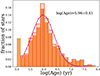 |
Fig. 10. Fraction of stellar ages derived from HR diagram for stars with log(Teff) < 3.73. The filled orange histogram shows the distribution of the whole sample, while the hatched red histogram represents the fraction distribution after removing the extreme bars with respect to the total number of stars within the new age range. The normal fit to the probability density distribution converted into the fraction distribution for the visual purposes is shown as a dark violet curve with a mean value of log(age) = 5.96 ± 0.41, corresponding to the 0.9 |

We checked how our conclusion on the cluster age is impacted when using different set of models. Therefore, we employed tracks from Baraffe et al. (2015) for low-mass stars (spectral types later than K5), and since they are limited to the solar-mass stars, for hotter stars we employed tracks from Siess et al. (2000). We present the HR diagram, the stellar properties, and a comparison between those two set of tracks in Appendix H. Those stellar parameters (M* and age) are also listed in Tables 1 and D.1. Use of different models changes the value of parameters for individual stars, but does not affect our conclusion on the cluster age. We performed the same exercise as described above for a distribution of stellar ages based on Baraffe et al. (2015)/Siess et al. (2000) evolutionary tracks. The normal fit indicates a cluster age of log(age) = 6.16 ± 0.31, corresponding to 1.4 Myr, consistent within errors to the previous estimate. Stellar, and hence cluster, ages around 1 Myr are difficult to infer precisely. We adopted that the age of Tr 14 is ∼1 Myr. This is a robust result (given uncertainties related to differences in models and internal uncertainties of observations) since the estimate is not affected by the choice of evolutionary tracks.
The large spread in the HR diagram seen in Tr 14 led in the past to conclusions of long, continuous star formation over the last 10 Myr (DeGioia-Eastwood et al. 2001; Povich et al. 2019), 1−6 Myr (Tapia et al. 2003), or 5 Myr (Ascenso et al. 2007). While comparing different clusters in Carina, Damiani et al. (2017) states that Tr 14 is younger than Trumpler 16, similarly to Smith & Brooks (2008), who found an age difference of 1−2 Myr between these two clusters. More precise estimates indicate an age for Trumpler 14 of 2 ± 1 Myr (Preibisch et al. 2011b). Rochau et al. (2011) found a recent (1.0 ± 0.5 Myr) starburst-like event and a hint of the presence of an older (3 Myr) population in Tr 14, which might be part of the dispersed population of the CNC. Overall, our estimate is in line with general findings in the literature. Our measurements also show a large spread of isochronal ages, which is a direct consequence of the luminosity spread. In the previous Sect. 4.2 we listed several possible sources responsible for the spread in luminosity within the stellar population of Tr 14, with the uncertainty of the parameters estimated during spectral classification expected to have the strongest impact. It is important to note that the aforementioned studies were mostly focused on massive and intermediate-mass stars (≳1 M⊙), while here we do not analyse stars hotter than ∼5500 K.
Additionally to the spread, Fig. 9 also shows a decrease in median luminosities towards hotter stars and a deviation from the ∼1 Myr isochrone, with the last temperature bin above log(Teff) ∼ 3.73 exhibiting a significant drop in luminosity. This behaviour could be caused by our selection bias as we focus on low-mass objects and do not identify in this work stars with spectral classes earlier than G8. This might result in the apparent “older” population of hotter stars. Hartmann (2003) noted a similar trend in the Taurus star-forming region. Stars colder than 4350 K (corresponding to the masses below ∼1 M⊙) had an age distribution strongly pointing to the values < 2 Myr, while hotter stars exhibited a flat distribution spanning up to 22 Myr (Hartmann 2003, see their Fig. 1). If we divide the age distributions into the same Teff ranges, we do not see such a strong behaviour – both sub-samples peak around 1 Myr – although we note that the youngest stars (≤0.15 Myr) are among those with Teff < 4350 K. Hartmann (2003) argued that the flat distribution of hotter Taurus members is due to the highly inaccurate positions of the birth line for the more massive stars, as well as non-member contamination. Similarly, Fang et al. (2017) shows that cluster ages are higher when derived from the luminosities and temperatures of hotter stars. The behaviour holds for different theoretical models and different young clusters. This effect could also impact our results.
Our observations span prominent, dense and compact cluster core (r ∼ 0.5′–0.9′, Ascenso et al. 2007; Kharchenko et al. 2013), and extended area around. The widely dispersed population of the CNC members (Feigelson et al. 2011; Zeidler et al. 2016) is mixed in our observations with the Tr 14 members causing the apparent age spread. We investigate that possibility below.
In Fig. 11 we mark the “core” area with radius 0.9′ and compare it to the location of our sources. We do not detect many sources in the most central area due to the spectral contamination. We investigate whether the stars inside the core have different properties than the population at larger radii from the cluster centre. Figure 12 shows de-reddened CMDs where sources inside (left panel) and outside (right panel) the radius of 0.9′ are marked with red hexagons. The core population of Tr 14 is mostly concentrated around the 1 Myr isochrone. Although the extended, “halo”, population exhibits larger spread in colours and ages, most of the stars are also located around the 1 Myr isochrone. Faint stars that are affected by the higher observational uncertainties are more numerous in this group. It is likely that the “halo” population is a mixture of young Tr 14 members and the older widely distributed population of the whole CNC. Since the widely distributed population of young stars in the CNC exhibits a range of ages between < 1 Myr and ∼8 Myr (Preibisch et al. 2011a), it is not possible with the available data to distinguish between Tr 14 members in the outer parts of the cluster and stars from the distributed population.
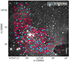 |
Fig. 11. Locations of the Li 6708 Å detections in the MUSE field (blue crosses). All the stars studied here are marked with red dots, as in Fig. 1. The dashed circle with a radius of 0.9′ shows the core of Tr 14, as defined by Kharchenko et al. (2013). The background image in grey-scale is the H-band image from HAWK-I (Preibisch et al. 2011a,b). |
We additionally checked the spatial distribution of young stars using the LiI 6708 Å absorption line. In Figs. 11 and 12 the stars where lithium was detected are marked with blue crosses. We do not find any specific concentration in the cluster of those stars but they all follow the < 10 Myr isochrones, as is expected for lithium-bearing stars. We note similar behaviour for NIR excess or X-ray emitting sources (see Appendix I). We conclude that in our dataset, where the most central core part is saturated and we cannot characterise most of the stars located there, the true, young members of Tr 14 are distributed evenly across the cluster. However, our sample also contains a number of stars from the widely distributed Carina population. We can neither distinguish between the true and apparent Tr 14 members nor confirm the cluster membership of older stars.
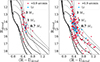 |
Fig. 12. Colour-magnitude diagrams for de-reddened R and I band magnitudes from MUSE. Red hexagons mark the stars within the core of Tr 14 (left, 0.9′, Kharchenko et al. 2013) or outside (right). The blue crosses indicate the location of the lithium-bearing stars on the CMDs within and outside the core radius, respectively. The same tracks are plotted as in Fig. 8. |
4.4. Mass distribution
Whether the environment can affect the IMF of the stellar cluster has been investigated in multiple studies. For example, Damian et al. (2021) studied low-mass stars in eight young clusters (∼2−3 Myr) observed in the J and K bands spanning a wide range of FUV radiation levels, cluster densities, and galactocentric distances. Their log-normal IMFs (Chabrier 2003) agreed well with each other, peaking within the range 0.2−0.4 M⊙ and not revealing any dependence on any of the three environmental properties. On the other hand, De Marchi et al. (2010) suggested that the present-day characteristic mass of the IMF is significantly correlated with the dynamical age of the cluster.
There has been no study dedicated to investigating the impact of the high FUV field on the IMF in the CNC. Only Rochau et al. (2011) tried to look at the mass function in the closest vicinity of the massive stars in Tr 14, but they could not draw any binding conclusions on their impact onto neighbouring stars. Similarly, Rainot et al. (2022) studied low-mass companions in the vicinity of seven O-type stars with the VLT/SPHERE in K-band. Despite the found differences between their IMF and the one from Rochau et al. (2011) or Chabrier (2003), they could not robustly confirm if the presence of the massive stars impacts their neighbouring companions or if the noticed differences are due to the observational bias. Former IMF studies in Tr 14 (e.g. Ascenso et al. 2007; Hur et al. 2012) were also based mostly on NIR photometry. Up to date no study has employed spectroscopy in Tr 14 to investigate the stellar mass distribution.
Our work focuses on low-mass stars with a spectral type later than G8. Figure 13 presents the distribution of stellar masses estimated based on MUSE observations in Tr 14 for stars with log(Teff) below 3.73. The shown masses range from 0.17 to 2.08 M⊙. The presented distribution is not an IMF as we did not correct for the photometric incompleteness. As we discussed in Sect. 2.3, the completeness of our catalogue is affected by crowdedness in the cluster core, the presence of bright stars, and highly variable nebular emission. According to the J band magnitude distribution in Fig. 2, we reach a 50% completeness level at 15.5 mag, corresponding to 0.8 M⊙ at 1 Myr (Bressan et al. 2012; Baraffe et al. 2015). However, if we include detections excluded from our catalogue due to the variable background emission, the 50% completeness level is already achieved at 18.5 mag (equivalent to 0.1 M⊙), demonstrating the depth and value of our MUSE data. In the second panel of Fig. 13 we show the fraction of stars in mass bins in the final (clean) catalogue in comparison to the sample without applying the background cut (Sect. 2.2.4). In the mass range below ∼0.8 M⊙ more than 50% detections are missing due to our conservative approach to background contamination. At the same time, none of the stars with masses ≳2.3 M⊙ were removed due to the high background variation. In Table D.1 we list targets with uncertain photometry and their stellar parameters, where available. Removing the lowest-mass stars from our catalogue prevents us from constructing an IMF estimate and identifying the characteristic mass of the Tr 14 population. More than half of the stars with masses < 0.8 M⊙ were removed from the final catalogue due the highly variable background (Fig. 13) but the proper completeness analysis is beyond the goal of this work. We note however that, when using a combined set of Baraffe et al. (2015) and Siess et al. (2000) evolutionary tracks, the distribution of masses is similar, although stellar masses extend only up to 4.1 M⊙. While the global picture of stellar mass distribution in Tr 14 is not affected by the choice of evolutionary models, the individual values can be different even by a factor of a few, especially for the least massive objects. This illustrates how challenging it is to derive accurate properties for young, low-mass stars.
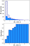 |
Fig. 13. Distribution of stellar masses in Tr 14 for stars with log(Teff) < 3.73. Top: filled histograms present the distribution of the masses of stars analysed in this paper. On top of it (hatched histogram) we display the distribution of the probable members with uncertain photometry removed from the analysis due to the high variability of the background emission. As is expected, most of the removed stars are faint, low-mass objects. Bottom: fraction of stars in the final spectroscopic catalogue within each mass bin relative to the combined catalogues of the final sample and probable members with uncertain photometry due to the variable background emission. The bins are the same as in the upper panel. |
The (in)variance of the IMF in the high FUV environment is also outside the scope of this paper. Future work addressing this problem needs first to resolve the completeness issue. Including more massive stars will enable an investigation of the slope of the mass function at the high-mass end. A more sophisticated approach to the estimation of the background emission may allow including significantly more low-mass stars and with that testing the breaking point of the Kroupa-like IMF or the characteristic mass of the log-normal IMF. High-spatial-resolution observations (e.g. with adaptive optics) of the very centre of Tr 14 could help to resolve the inner core region. Brown dwarfs and very low-mass members of Tr 14 can only be well spectroscopically characterised by NIR IFU instruments, like VLT/KMOS, VLT/ERIS, JWST/NIRspec, or the future ELT/HARMONI.
5. Summary and conclusions
In this work, we present the first optical spectroscopic study of low-mass stars in Tr 14 based on IFU observations from VLT/MUSE. We identified targets and extracted photometry and spectra using SExtractor. We excluded from the catalogue all sources with uncertain photometry. Specifically, the most significant cut (of 1868 sources) was related to the emission of the HII region in the CNC, which is highly variable in the spatial dimension. In the end, our catalogue consists of 780 stars. We make available both catalogues, with robust and uncertain photometry, for possible future follow-up studies.
Most of our sources have photometric measurements from NIR (99%) and optical (76%) catalogues, and almost 40% were detected in X-rays. We performed the spectral classification using spectra of Class III stars from Manara et al. (2013, 2017) as templates. Together with the spectral type we estimated visual reddening and constant veiling of 717 stars. We converted the spectral types to the effective temperatures and used J band photometry to calculate bolometric luminosities. We placed our stars in the HR diagram and by a comparison to the theoretical evolutionary tracks (Bressan et al. 2012) we estimated the stellar masses and ages. Based on the distribution of the stellar ages we estimated the cluster age of ∼1 Myr. This result is maintained even when using different evolutionary models (Siess et al. 2000; Baraffe et al. 2015). The majority of our stars (51%) have a mass below 1 M⊙, while the least massive object has an estimated mass of 0.17 M⊙.
Massive star-forming regions represent the most common environment in which stars form in the Galaxy. This environment differs from those seen in the solar neighbourhood and therefore necessitates an extension of the study of more distant regions. Those examinations are however challenging due to the large distance to the cluster, often high extinction, and high stellar crowding. This is particularly difficult for spectroscopic observations. Here, we present that those kinds of explorations are feasible with IFU spectrographs like VLT/MUSE. Low-mass stars are the most common in the Galaxy but at the same time the most vulnerable to environmental conditions. The stellar characteristics presented here of a few hundred of low-mass stars provide a step towards a better understanding of the formation and early evolution of low-mass stars in the massive cluster. This study sets a foundation for the follow-up investigation of the protoplanetary disc population response to the high FUV field in the cluster that will be presented in a consecutive paper.
The full description of SExtractor flags is available on the website at https://sextractor.readthedocs.io/en/latest/Flagging.html#flags-def
Acknowledgments
We thank the referee, Guido De Marchi, for a careful reading and for insightful comments helping improving this manuscript. This work was partly supported by the Italian Ministero dell’Istruzione, Università e Ricerca through the grant Progetti Premiali 2012-iALMA (CUP C52I13000140001), by the Deutsche Forschungsgemeinschaft (DFG, German Research Foundation) – Ref. no. 325594231 FOR 2634/2 TE 1024/2-1, by the DFG Cluster of Excellence Origins (https://www.origins-cluster.de), by the Fondazione Cariplo, grant no. 2022-1217. This project has received funding from the European Union’s Horizon 2020 research and innovation program under the Marie Skłodowska Curie grant agreement No. 823823 (DUSTBUSTERS), from the European Research Council (ERC) via the ERC Synergy Grant ECOGAL (grant 855130), and by the European Union (ERC, WANDA, 101039452 and ERC, DiscEvol, 101039651). Views and opinions expressed are however those of the author(s) only and do not necessarily reflect those of the European Union or the European Research Council Executive Agency. Neither the European Union nor the granting authority can be held responsible for them. This work has made use of data from the European Space Agency (ESA) mission Gaia (https://www.cosmos.esa.int/gaia), processed by the Gaia Data Processing and Analysis Consortium (DPAC, https://www.cosmos.esa.int/web/gaia/dpac/consortium). Funding for the DPAC has been provided by national institutions, in particular the institutions participating in the Gaia Multilateral Agreement.
References
- Adams, F. C. 2010, ARA&A, 48, 47 [NASA ADS] [CrossRef] [Google Scholar]
- Adams, F. C., Hollenbach, D., Laughlin, G., & Gorti, U. 2004, ApJ, 611, 360 [NASA ADS] [CrossRef] [Google Scholar]
- Albacete-Colombo, J. F., Damiani, F., Micela, G., Sciortino, S., & Harnden, F. R., Jr. 2008, A&A, 490, 1055 [NASA ADS] [CrossRef] [EDP Sciences] [Google Scholar]
- Alcalá, J. M., Natta, A., Manara, C. F., et al. 2014, A&A, 561, A2 [NASA ADS] [CrossRef] [EDP Sciences] [Google Scholar]
- Allington-Smith, J., Murray, G., Content, R., et al. 2002, PASP, 114, 892 [NASA ADS] [CrossRef] [Google Scholar]
- Almendros-Abad, V., Mužić, K., Bouy, H., et al. 2023, A&A, 677, A26 [NASA ADS] [CrossRef] [EDP Sciences] [Google Scholar]
- Anderson, K. R., Adams, F. C., & Calvet, N. 2013, ApJ, 774, 9 [NASA ADS] [CrossRef] [Google Scholar]
- Antokhin, I. I., Rauw, G., Vreux, J. M., van der Hucht, K. A., & Brown, J. C. 2008, A&A, 477, 593 [NASA ADS] [CrossRef] [EDP Sciences] [Google Scholar]
- Ascenso, J., Alves, J., Vicente, S., & Lago, M. T. V. T. 2007, A&A, 476, 199 [NASA ADS] [CrossRef] [EDP Sciences] [Google Scholar]
- Bacon, R., Accardo, M., Adjali, L., et al. 2010, in Ground-based and Airborne Instrumentation for Astronomy III, eds. I. S. McLean, S. K. Ramsay, & H. Takami, SPIE Conf. Ser., 7735, 773508 [Google Scholar]
- Baraffe, I., Chabrier, G., & Gallardo, J. 2009, ApJ, 702, L27 [NASA ADS] [CrossRef] [Google Scholar]
- Baraffe, I., Homeier, D., Allard, F., & Chabrier, G. 2015, A&A, 577, A42 [NASA ADS] [CrossRef] [EDP Sciences] [Google Scholar]
- Beccari, G., De Marchi, G., Panagia, N., et al. 2015, A&A, 574, A44 [NASA ADS] [CrossRef] [EDP Sciences] [Google Scholar]
- Berlanas, S. R., Maíz Apellániz, J., Herrero, A., et al. 2023, A&A, 671, A20 [NASA ADS] [CrossRef] [EDP Sciences] [Google Scholar]
- Bertin, E., & Arnouts, S. 1996, A&AS, 117, 393 [NASA ADS] [CrossRef] [EDP Sciences] [Google Scholar]
- Bressan, A., Marigo, P., Girardi, L., et al. 2012, MNRAS, 427, 127 [NASA ADS] [CrossRef] [Google Scholar]
- Broos, P. S., Townsley, L. K., Feigelson, E. D., et al. 2011, ApJS, 194, 2 [NASA ADS] [CrossRef] [Google Scholar]
- Cantat-Gaudin, T., Jordi, C., Vallenari, A., et al. 2018, A&A, 618, A93 [NASA ADS] [CrossRef] [EDP Sciences] [Google Scholar]
- Cardelli, J. A., Clayton, G. C., & Mathis, J. S. 1989, ApJ, 345, 245 [Google Scholar]
- Carpenter, J. M., Hillenbrand, L. A., & Skrutskie, M. F. 2001, AJ, 121, 3160 [NASA ADS] [CrossRef] [Google Scholar]
- Carraro, G., Romaniello, M., Ventura, P., & Patat, F. 2004, A&A, 418, 525 [NASA ADS] [CrossRef] [EDP Sciences] [Google Scholar]
- Chabrier, G. 2003, ApJ, 586, L133 [NASA ADS] [CrossRef] [Google Scholar]
- Chen, Y., Girardi, L., Bressan, A., et al. 2014, MNRAS, 444, 2525 [Google Scholar]
- Claes, R. A. B., Manara, C. F., Garcia-Lopez, R., et al. 2022, A&A, 664, L7 [NASA ADS] [CrossRef] [EDP Sciences] [Google Scholar]
- Costigan, G., Scholz, A., Stelzer, B., et al. 2012, MNRAS, 427, 1344 [Google Scholar]
- Costigan, G., Vink, J. S., Scholz, A., Ray, T., & Testi, L. 2014, MNRAS, 440, 3444 [NASA ADS] [CrossRef] [Google Scholar]
- Cox, A. N. 2000, Allen’s Astrophysical Quantities (New York: AIP Press) [Google Scholar]
- Damian, B., Jose, J., Samal, M. R., et al. 2021, MNRAS, 504, 2557 [NASA ADS] [CrossRef] [Google Scholar]
- Damiani, F., Klutsch, A., Jeffries, R. D., et al. 2017, A&A, 603, A81 [NASA ADS] [CrossRef] [EDP Sciences] [Google Scholar]
- Davies, R., Absil, O., Agapito, G., et al. 2023, A&A, 674, A207 [NASA ADS] [CrossRef] [EDP Sciences] [Google Scholar]
- DeGioia-Eastwood, K., Throop, H., Walker, G., & Cudworth, K. M. 2001, ApJ, 549, 578 [CrossRef] [Google Scholar]
- De Marchi, G., Paresce, F., & Portegies Zwart, S. 2010, ApJ, 718, 105 [NASA ADS] [CrossRef] [Google Scholar]
- Duchêne, G., & Kraus, A. 2013, ARA&A, 51, 269 [Google Scholar]
- Eisner, J. A., Arce, H. G., Ballering, N. P., et al. 2018, ApJ, 860, 77 [CrossRef] [Google Scholar]
- Facchini, S., Clarke, C. J., & Bisbas, T. G. 2016, MNRAS, 457, 3593 [NASA ADS] [CrossRef] [Google Scholar]
- Fang, Q., Herczeg, G. J., & Rizzuto, A. 2017, ApJ, 842, 123 [Google Scholar]
- Fang, M., Kim, J. S., Pascucci, I., & Apai, D. 2021, ApJ, 908, 49 [NASA ADS] [CrossRef] [Google Scholar]
- Feigelson, E. D., Getman, K. V., Townsley, L. K., et al. 2011, ApJS, 194, 9 [Google Scholar]
- Feinstein, A., Marraco, H. G., & Muzzio, J. C. 1973, A&AS, 12, 331 [NASA ADS] [Google Scholar]
- Fischer, W. J., Hillenbrand, L. A., Herczeg, G. J., et al. 2023, in Astronomical Society of the Pacific Conference Series, eds. S. Inutsuka, Y. Aikawa, T. Muto, K. Tomida, & M. Tamura, ASP Conf. Ser., 534, 355 [NASA ADS] [Google Scholar]
- Freudling, W., Romaniello, M., Bramich, D. M., et al. 2013, A&A, 559, A96 [NASA ADS] [CrossRef] [EDP Sciences] [Google Scholar]
- Freyer, T., Hensler, G., & Yorke, H. W. 2003, ApJ, 594, 888 [NASA ADS] [CrossRef] [Google Scholar]
- Gaia Collaboration (Prusti, T., et al.) 2016, A&A, 595, A1 [NASA ADS] [CrossRef] [EDP Sciences] [Google Scholar]
- Gaia Collaboration (Vallenari, A., et al.) 2023, A&A, 674, A1 [NASA ADS] [CrossRef] [EDP Sciences] [Google Scholar]
- Göppl, C., & Preibisch, T. 2022, A&A, 660, A11 [NASA ADS] [CrossRef] [EDP Sciences] [Google Scholar]
- Gritschneder, M., Burkert, A., Naab, T., & Walch, S. 2010, ApJ, 723, 971 [Google Scholar]
- Hartmann, L. 2001, AJ, 121, 1030 [NASA ADS] [CrossRef] [Google Scholar]
- Hartmann, L. 2003, ApJ, 585, 398 [NASA ADS] [CrossRef] [Google Scholar]
- Haworth, T. J., & Harries, T. J. 2012, MNRAS, 420, 562 [NASA ADS] [CrossRef] [Google Scholar]
- Herczeg, G. J., & Hillenbrand, L. A. 2014, ApJ, 786, 97 [Google Scholar]
- Hur, H., Sung, H., & Bessell, M. S. 2012, AJ, 143, 41 [NASA ADS] [CrossRef] [Google Scholar]
- Hur, H., Lim, B., & Chun, M.-Y. 2023, J. Korean Astron. Soc., 56, 97 [NASA ADS] [Google Scholar]
- Jeffries, R. D., Oliveira, J. M., Naylor, T., Mayne, N. J., & Littlefair, S. P. 2007, MNRAS, 376, 580 [NASA ADS] [CrossRef] [Google Scholar]
- Kenyon, S. J., & Hartmann, L. 1995, ApJS, 101, 117 [Google Scholar]
- Kharchenko, N. V., Piskunov, A. E., Schilbach, E., Röser, S., & Scholz, R. D. 2013, A&A, 558, A53 [NASA ADS] [CrossRef] [EDP Sciences] [Google Scholar]
- Köhler, R., Neuhäuser, R., Krämer, S., et al. 2008, A&A, 488, 997 [NASA ADS] [CrossRef] [EDP Sciences] [Google Scholar]
- Krumholz, M. R., Klein, R. I., & McKee, C. F. 2011, ApJ, 740, 74 [NASA ADS] [CrossRef] [Google Scholar]
- Lada, C. J., & Lada, E. A. 2003, ARA&A, 41, 57 [Google Scholar]
- Leinert, C., Zinnecker, H., Weitzel, N., et al. 1993, A&A, 278, 129 [NASA ADS] [Google Scholar]
- Levato, H., & Malaroda, S. 1982, PASP, 94, 807 [NASA ADS] [CrossRef] [Google Scholar]
- Lindegren, L. 2018, Re-normalising the Astrometric Chi-square in Gaia DR2 (Lund Observatory) [Google Scholar]
- Lindegren, L., Bastian, U., Biermann, M., et al. 2021, A&A, 649, A4 [EDP Sciences] [Google Scholar]
- Luhman, K. L. 1999, ApJ, 525, 466 [Google Scholar]
- Luhman, K. L., Stauffer, J. R., Muench, A. A., et al. 2003, ApJ, 593, 1093 [Google Scholar]
- Maíz Apellániz, J., Sota, A., Arias, J. I., et al. 2016, ApJS, 224, 4 [CrossRef] [Google Scholar]
- Maíz Apellániz, J., Crespo Bellido, P., Barbá, R. H., Fernández Aranda, R., & Sota, A. 2020, A&A, 643, A138 [NASA ADS] [CrossRef] [EDP Sciences] [Google Scholar]
- Manara, C. F., Testi, L., Rigliaco, E., et al. 2013, A&A, 551, A107 [NASA ADS] [CrossRef] [EDP Sciences] [Google Scholar]
- Manara, C. F., Frasca, A., Alcalá, J. M., et al. 2017, A&A, 605, A86 [NASA ADS] [CrossRef] [EDP Sciences] [Google Scholar]
- Manara, C. F., Ansdell, M., Rosotti, G. P., et al. 2023, ASP Conf. Ser., 534, 539 [NASA ADS] [Google Scholar]
- Marmo, C., & Bertin, E. 2008, in Astronomical Data Analysis Software and Systems XVII, eds. R. W. Argyle, P. S. Bunclark, & J. R. Lewis, ASP Conf. Ser., 394, 619 [Google Scholar]
- Massey, P., & Johnson, J. 1993, AJ, 105, 980 [Google Scholar]
- McGregor, P. J., Hart, J., Conroy, P. G., et al. 2003, in Instrument Design and Performance for Optical/Infrared Ground-based Telescopes, eds. M. Iye, & A. F. M. Moorwood, Proc. SPIE, 4841, 178 [NASA ADS] [Google Scholar]
- Miller, G. E., & Scalo, J. M. 1978, PASP, 90, 506 [NASA ADS] [CrossRef] [Google Scholar]
- Morrell, N., Garcia, B., & Levato, H. 1988, PASP, 100, 1431 [CrossRef] [Google Scholar]
- O’Dell, C. R., Wen, Z., & Hu, X. 1993, ApJ, 410, 696 [CrossRef] [Google Scholar]
- Oliveira, J. M., Jeffries, R. D., Devey, C. R., et al. 2003, MNRAS, 342, 651 [NASA ADS] [CrossRef] [Google Scholar]
- Parker, R. J. 2020, R. Soc. Open Sci., 7, 201271 [NASA ADS] [CrossRef] [Google Scholar]
- Penny, L. R., Gies, D. R., Hartkopf, W. I., Mason, B. D., & Turner, N. H. 1993, PASP, 105, 588 [NASA ADS] [CrossRef] [Google Scholar]
- Peterson, D. E., Megeath, S. T., Luhman, K. L., et al. 2008, ApJ, 685, 313 [CrossRef] [Google Scholar]
- Pfalzner, S., Davies, M. B., Gounelle, M., et al. 2015, Phys. Scr., 90, 068001 [NASA ADS] [CrossRef] [Google Scholar]
- Povich, M. S., Smith, N., Majewski, S. R., et al. 2011, ApJS, 194, 14 [Google Scholar]
- Povich, M. S., Maldonado, J. T., Nuñez, E. H., & Robitaille, T. P. 2019, ApJ, 881, 37 [NASA ADS] [CrossRef] [Google Scholar]
- Preibisch, T., Hodgkin, S., Irwin, M., et al. 2011a, ApJS, 194, 10 [Google Scholar]
- Preibisch, T., Ratzka, T., Kuderna, B., et al. 2011b, A&A, 530, A34 [NASA ADS] [CrossRef] [EDP Sciences] [Google Scholar]
- Preibisch, T., Roccatagliata, V., Gaczkowski, B., & Ratzka, T. 2012, A&A, 541, A132 [NASA ADS] [CrossRef] [EDP Sciences] [Google Scholar]
- Preibisch, T., Zeidler, P., Ratzka, T., Roccatagliata, V., & Petr-Gotzens, M. G. 2014, A&A, 572, A116 [NASA ADS] [CrossRef] [EDP Sciences] [Google Scholar]
- Preibisch, T., Flaischlen, S., Göppl, C., Ercolano, B., & Roccatagliata, V. 2021, A&A, 648, A34 [NASA ADS] [CrossRef] [EDP Sciences] [Google Scholar]
- Qiao, L., Coleman, G. A. L., & Haworth, T. J. 2023, MNRAS, 522, 1939 [NASA ADS] [CrossRef] [Google Scholar]
- Rainot, A., Reggiani, M., Sana, H., Bodensteiner, J., & Absil, O. 2022, A&A, 658, A198 [NASA ADS] [CrossRef] [EDP Sciences] [Google Scholar]
- Riddick, F. C., Roche, P. F., & Lucas, P. W. 2007, MNRAS, 381, 1067 [Google Scholar]
- Rochau, B., Brandner, W., Stolte, A., et al. 2011, MNRAS, 418, 949 [NASA ADS] [CrossRef] [Google Scholar]
- Rowles, J., & Froebrich, D. 2009, MNRAS, 395, 1640 [CrossRef] [Google Scholar]
- Sharples, R., Bender, R., Agudo Berbel, A., et al. 2013, The Messenger, 151, 21 [NASA ADS] [Google Scholar]
- Shull, J. M., Darling, J., & Danforth, C. W. 2021, ApJ, 914, 18 [NASA ADS] [CrossRef] [Google Scholar]
- Siess, L., Dufour, E., & Forestini, M. 2000, A&A, 358, 593 [Google Scholar]
- Smith, N. 2002, MNRAS, 337, 1252 [NASA ADS] [CrossRef] [Google Scholar]
- Smith, N. 2006, MNRAS, 367, 763 [Google Scholar]
- Smith, N., & Brooks, K. J. 2008, in Handbook of Star Forming Regions, Volume II, ed. B. Reipurth, 5, 138 [NASA ADS] [Google Scholar]
- Tapia, M., Roth, M., Vázquez, R. A., & Feinstein, A. 2003, MNRAS, 339, 44 [CrossRef] [Google Scholar]
- Throop, H. B., & Bally, J. 2005, ApJ, 623, L149 [NASA ADS] [CrossRef] [Google Scholar]
- Townsley, L. K., Broos, P. S., Corcoran, M. F., et al. 2011, ApJS, 194, 1 [Google Scholar]
- Vaidya, K., Chen, W.-P., & Lee, H.-T. 2015, AJ, 150, 195 [NASA ADS] [CrossRef] [Google Scholar]
- Vazquez, R. A., Baume, G., Feinstein, A., & Prado, P. 1996, A&AS, 116, 75 [NASA ADS] [Google Scholar]
- Venuti, L., Bouvier, J., Flaccomio, E., et al. 2014, A&A, 570, A82 [NASA ADS] [CrossRef] [EDP Sciences] [Google Scholar]
- Walborn, N. R. 1973, ApJ, 179, 517 [NASA ADS] [CrossRef] [Google Scholar]
- Walborn, N. R. 1995, in Rev. Mex. Astron. Astrof. Conf. Ser., eds. V. Niemela, N. Morrell, & A. Feinstein, 2, 51 [NASA ADS] [Google Scholar]
- Walborn, N. R., Howarth, I. D., Lennon, D. J., et al. 2002, AJ, 123, 2754 [NASA ADS] [CrossRef] [Google Scholar]
- Weilbacher, P. M., Palsa, R., Streicher, O., et al. 2020, A&A, 641, A28 [NASA ADS] [CrossRef] [EDP Sciences] [Google Scholar]
- Whitworth, A. P., & Zinnecker, H. 2004, A&A, 427, 299 [NASA ADS] [CrossRef] [EDP Sciences] [Google Scholar]
- Winter, A. J., & Haworth, T. J. 2022, Eur. Phys. J. Plus, 137, 1132 [NASA ADS] [CrossRef] [Google Scholar]
- Winter, A. J., Clarke, C. J., Rosotti, G., et al. 2018, MNRAS, 478, 2700 [Google Scholar]
- Winter, A. J., Kruijssen, J. M. D., Longmore, S. N., & Chevance, M. 2020, Nature, 586, 528 [Google Scholar]
- Zagaria, F., Clarke, C. J., Rosotti, G. P., & Manara, C. F. 2022, MNRAS, 512, 3538 [NASA ADS] [CrossRef] [Google Scholar]
- Zeidler, P., Preibisch, T., Ratzka, T., Roccatagliata, V., & Petr-Gotzens, M. G. 2016, A&A, 585, A49 [NASA ADS] [CrossRef] [EDP Sciences] [Google Scholar]
- Zurlo, A., Cieza, L. A., Pérez, S., et al. 2020, MNRAS, 496, 5089 [Google Scholar]
- Zurlo, A., Gratton, R., Pérez, S., & Cieza, L. 2023, Eur. Phys. J. Plus, 138, 411 [NASA ADS] [CrossRef] [Google Scholar]
Appendix A: Observational log
In Table A.1 we provide basic information about weather conditions during observations with “long” integration times (3×13 min) and the name of the standard star used for the flux calibration for each set. Due to bad atmospheric conditions some observations were repeated. We checked all datasets and used those that were described as better quality by the observatory. We include in the table all observations made for use by the astronomical community.
Observational log.
Appendix B: Coordinates correction and cross-match with photometric catalogues
We corrected the MUSE coordinates using the Gaia DR3 catalogue (Gaia Collaboration 2023). The applied corrections are median differences in the right ascension and declination between MUSE and Gaia. We show the distribution of those differences for each pointing in Figure B.1. Corrections that need to be added to the original MUSE coordinates are listed in Table B.1. They range in absolute values between 1.46″ and 5.75″ for the right ascension, and between 0.08″ and 2.98″ for the declination, with a typical STD of 0.15″ for the right ascension and 0.08″ for the declination.
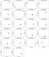 |
Fig. B.1. Distribution of differences in right ascensions and declinations from MUSE and Gaia DR3 at each field. |
Applied coordinate offsets.
After correcting MUSE coordinates, we again matched our sources with Gaia to examine the accuracy of our astrometry and define the best matching radius between different catalogues. Based on the bimodal distribution of separations between corrected MUSE and Gaia coordinates in Figure B.2, we find that the best separation radius for cross-matching is 0.5″. Within it we find all true counterparts and do not include false matches with larger separations. False matches are caused by crowding, especially large in the cluster centre. The same distribution shows that the uncertainty of our astrometry is ∼0.1″.
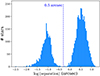 |
Fig. B.2. Separations in arcsec between MUSE and Gaia DR3 stars on a logarithmic scale. The MUSE catalogue here contains data points as of Sec. 2.2.1, before removing uncertain photometry. Overplotted is the threshold separation of 0.5″ used in this work. |
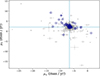 |
Fig. B.3. Proper motions of Gaia counterparts. We show points with available proper motion measurements (grey dots) and with good astrometry (dark blue circles) (see Sec. 2.2.6 for details). Uncertainties of the latter points are smaller than the symbol sizes. Foreground and possibly contaminated stars are excluded. For reference, we also mark group proper motions from Berlanas et al. (2023) derived from Gaia EDR3 astrometry of OB stars in Tr 14. |
Appendix C: Targets detected in more than one pointing
The pointings of observations were designed to overlap. Therefore, some stars were detected multiple times in several pointings. After coordinate correction, we identified those targets performing coordinate matching within the catalogue. We defined the same separation limit of 0.5″, below which we assumed that the two detections corresponded to the same object. We find separations in the range from 0.09″ to 0.26″ with a median of 0.20″ corresponding to the size of one pixel. In Table C.1 we list all the pairs of double detections.
Twice-detected sources.
In most cases the I band magnitudes of both detections are consistent within the uncertainties. That reassures us about the overall good inter-frame calibration. We chose a S/N in the vicinity of 7500 Å (snr750) as a measure of the quality and used in the analysis the spectrum with a higher snr750. In Figure C.1 we show a few examples of comparisons between the spectra of the two doubles. Corresponding snr750 are indicated in the legend of each panel. The difference between the spectra is particularly visible in the case of late-type stars. There, the blue part of the spectrum is very vulnerable to the quality of the spectrum. In general, we see no trend between the chosen spectra and weather conditions, although there is a slight preference towards better seeing. We also note that stars located very close to the detector’s edge were not detected by the SExtractor.
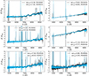 |
Fig. C.1. Examples of spectra observed twice. Spectra were normalised to the flux at 7500 Å. The label indicates the source identifier and its S/N of around 7500 Å which was used to decide which spectrum to keep for the analysis. |
Appendix D: Assessment of the background variability
SExtractor provides estimates of stellar fluxes, magnitudes, and sky emission at the positions of the stars. It assumes a smooth variation in the sky emission across the whole image. The tool does not provide uncertainty of the background estimation. Since some parts of the cluster covered by our observations are very crowded and the sky emission exhibits prominent gaseous structures, local variation in the sky emission might not be smooth. Therefore, we employ another strategy to assess the quality of stellar magnitudes and spectra.
We looked at the variation in the background emission estimated for each target by SExtractor within the defined area around each star. We checked that a circle with a radius of 20″ was large enough to cover a satisfactory number of neighbouring sources and, at the same time, small enough to cover only the “local” area. The left panel of Figure D.1 shows how many neighbouring sources for each star are within a radius of 20″. The distribution peaks at 40-50 neighbours, giving satisfactory large statistics. We calculated the STD of the sky emission within this area for every star in our catalogue. The right panel of the Fig. D.1 shows the distribution of the STD measured in flux units of erg s−1 cm−2 Å−1. We used such defined variability to select a robust photometry: we discarded the measurement of the stellar flux that is below the threshold of three sigma (here σ=std). We initially performed this exercise in the I band, as the presence of this magnitude is our definition of detection, and repeated it for the R and V bands. Since our stars have late spectroscopic types, they appear fainter in bluer bands, and therefore there are fewer photometric measurements in the R and V bands than in the I band. That can be noticed in our CMDs in Fig. 4 and 8. We note that our approach is very conservative: spectra of some of the removed targets from the final catalogue have a high enough S/N for spectral classification. For this reason, we listed in Table D.1 sources removed due to the uncertain photometry in the I band caused by the high background variation. We included in the table uncertain photometry from all bands. The columns “snrI,bkg”, “snrR,bkg”, and “snrV,bkg” show ratios between the stellar flux and the background variation in a given band, and therefore can be used as indicators of photometric certainty.
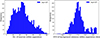 |
Fig. D.1. Left: Distribution of the number of sources within a separation of 20″ from a given star. Right: Distribution of the STD of background emission estimated in the I band from the individual measurements within 20″ of the given star. |
Parameters of stars removed from the catalogue due to the high background variation.
Appendix E: MUSE photometry
The MUSE I, R, and V band images in flux units were produced by collapsing the 3D MUSE cubes within the corresponding wavelength range and applying the filter transmission curve embedded in the ESO reduction pipeline (Weilbacher et al. 2020). We performed the aperture photometry with SExtractor, extracting stellar fluxes from the images and converting them to magnitudes using Vega zero points written in the headers by the pipeline. Even though our observations were flux-calibrated using standard stars, we found that our magnitudes deviate from those measured with the WFI by Beccari et al. (2015) (described below). As those measurements are well calibrated, we corrected the MUSE magnitudes so that they matched those from the WFI. We defined a correction as a difference between MUSE and WFI magnitudes and subtracted it from the MUSE photometry. Corrections for each field and each band are listed in the Table E.1. In the I band they range from 0.29 mag in field No. 5 to 1.27 mag in field No. 15. We also checked whether a colour term is present in MUSE photometry. Fig. E.1 shows an example of this examination, with the result of no colour term between the I and R bands.
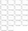 |
Fig. E.1. Difference between MUSE and WFI (Beccari et al. 2015) I band photometry as a function of MUSE colour R − I. Every panel represents a separate field, as indicated in the upper right corner. The dashed grey line shows the mean difference between I band magnitudes applied to MUSE photometry as magnitude correction. |
Photometric corrections.
The highest-value corrections are in fields No. 15, 12, and 19 (≳1.0 mag). Pointings 12 and 19 have the worst seeing from all used observations, which may explain the difference in the estimated flux. No. 12 suffers additionally from the presence of two very bright stars in the centre of the field, whose brightness impact all neighbouring stars in the image, possibly to a larger extent than assumed in this work. No. 15 is one of the most crowded pointings, although it does not cover the very centre of Tr 14. The presence of few bright stars and a prominent feature with a high extinction in the lower right corner of the field might be another explanation of the large magnitude difference. If, as the result, the background estimation from the SExtractor is incorrect, that would lead to the uncertain stellar photometry. Weather conditions were moderate (thin clouds), which might also have affected the observations.
The uncertainty of the magnitude corrections, measured as a STD of magnitude differences, is ∼0.1 mag for most of the pointings. It also usually increases towards the bluer bands. However, the smaller number of available magnitudes in bluer bands due to the high background variability could cause underestimation of those uncertainties. Overall, the offset of the MUSE magnitudes seem to be relatively constant within the pointing. We added linear correction uncertainties to the magnitude uncertainties of our sources and report them in the catalogues (Tab. 1 & D.1).
We show the resulting distributions of the corrected MUSE magnitudes in Figure E.2. The distribution of I band magnitudes peaks at 18.01 mag, R band at 17.60 mag, and V band at 17.58 mag. The number of magnitudes in each band decreases bluewards, from 780 in the I band through to 294 in the R band and 223 in the V band.
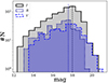 |
Fig. E.2. Distribution of corrected MUSE magnitudes. colours indicate different photometric bands as stated in the upper left corner of the figure. Dashed lines show the turn-over point of the distributions located at: 18.01 mag (I band), 17.60 mag (R band), 17.58 mag (V band). |
Appendix F: Spectral templates
Here, we list all Class III stars and their properties used in spectral classification as spectral templates (Table F.1). Spectral types for those stars later than K5 were obtained based on the depth of the molecular absorption bands (TiO, VO, and CaH) and a few photospheric lines (e.g. NaI, CaI, MgI, etc.) present in the optical part of the spectra (Manara et al. 2013). Earlier K-type stars were identified using the spectral indices introduced by Herczeg & Hillenbrand (2014), while G-type stars were identified based on the difference at 5150 Å of the continuum estimated between 4600 and 5400 Å, and 4900 and 5150 Å (Herczeg & Hillenbrand 2014). Effective temperatures (Teff) were derived from spectral types using relations from Luhman et al. (2003) for M-type objects and Kenyon & Hartmann (1995) for K- and G-type stars. Most of the templates have no, or only a negligible, extinction (AV < 0.5 mag, Manara et al. 2017); spectra were de-reddened before analysis assuming the extinction law from Cardelli et al. (1989) and RV = 3.1. All the details of the data reduction, calibration, and spectral classification are provided in the original papers.
Properties of Class III stars used as spectral templates.
Appendix G: Spectral classification
In this appendix, we list the spectral indices used for the spectral classification of K- and late G-type stars, and we explain in more detail the estimation of uncertainties based on  maps.
maps.
Indices were defined, calibrated, and tested on Class III spectra listed in the Table F.1. Each spectral index is defined as an equivalent width of a given line or a line ratio of the two. Table G.1 shows our indices together with their weights. The final spectral type is a weighted average of indices. Indices with values outside the applicable range of spectral types (indicating a type earlier than G8 or later than M0) were excluded from the average to avoid extrapolation. We required at least three valid indices to estimate the spectral type. Additionally, we included in our list the index from Oliveira et al. (2003), Jeffries et al. (2007), TiO 7140Å. It is applicable only to the stars with a spectral type later than K5.
Indices used for spectral classification of K- and late G-type stars.
Extinction and veiling at 7500Å, as well as the spectral type for M-type stars, were estimated based on  maps. Figure G.1 shows examples of such maps for an M-type star, and Figure G.2 for an K-type star. Each time, we examined the distribution of
  in relation to a given two out of three variables in our problem (spectral type, SpT; visual extinction, AV, and constant veiling at 7500 Å, r750). Hence, for M-type stars, there are three
  maps for each star. For K-type stars, where uncertainties of the spectral type are assigned differently, there is only one
  map constructed based on the Class III template closest with the SpT to the SpT of a given star. The best set of parameter values is indicated by the minimum value of the
  . The 1-sigma contours drawn on top of the distributions are the basis of the uncertainty estimates. We adopted the projections of the contours onto the axis as the uncertainties of the given parameters. Fig. G.1 and G.2 show 1-sigma contours, and additionally also 2- and 3-sigma ones, for reference.
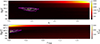 |
Fig. G.1. The |


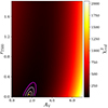 |
Fig. G.1. (cont.) The |

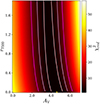 |
Fig. G.3. The |

Estimating uncertainties based on our  distributions is itself prone to uncertainty. The sampling of spectral templates used for classification does not even cause a discontinuous, step-like shape of 1-sigma contours. We did not propagate errors outside the range of adopted values for our parameters. As a result, when the best value is close to the edge of this range, one of the uncertainties will be underestimated. We observe a high degeneracy between veiling and extinction, as well as a high uncertainty of the value of the veiling, especially in hotter stars. Therefore, our veiling estimates might be inaccurate and we recommend that they be treated as rough indications of the presence of the veiling and its prominence.
Appendix H: Stellar parameters
The selection of stellar evolutionary models impacts the values of derived stellar parameters. In Section 4.2 we constructed an HR diagram and employed PARSEC v1.2S tracks (Bressan et al. 2012) to estimate the masses and ages of Tr 14 members. Here, we investigated how the choice of tracks impact our results on cluster properties. We used tracks developed for young stars from Siess et al. (2000) and Baraffe et al. (2015). The latter are dedicated to low- and very low-mass stars and therefore do not cover stars more massive than ∼1 M⊙. Thus, we combined them with tracks from Siess et al. (2000) and defined a border of spectral type K5 between usage of the two models. Neither model explores ages below 0.5 Myr. We restricted the comparison up to 30 Myr, as we do not expect true Tr 14 members to be that old.
We present the HR diagram in Figure H.1. A comparison with the HR diagram using PARSEC tracks in Figure 9 shows differences in stellar masses at the lower end. Figure H.2 compares mass distributions of the two sets of tracks. The distribution of PARSEC masses is shifted with respect to the Baraffe et al. (2015) and Siess et al. (2000) ones. The differences are the most prominent between PARSEC and Baraffe et al. (2015) models up to a factor of ∼2. Masses from PARSEC and Siess et al. (2000) seem to be consistent with some spread.
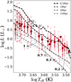 |
Fig. H.1. HR diagram for low-mass stars of Tr 14. Empty circles show data points. Open squares are median values of the bolometric luminosity for each spectral subclass, with error bars indicating 1-σ percentiles. Theoretical tracks from Baraffe et al. (2015) are shown as solid grey lines, whereas tracks from Siess et al. (2000) are plotted as dashed lines. Dotted lines show tracks for various masses of stars. |
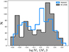 |
Fig. H.2. Distribution of all stellar masses from the final catalogue on a logarithmic scale. The black histogram filled with grey shows masses estimated based on evolutionary tracks from Baraffe et al. (2015) and Siess et al. (2000), while the open blue histogram shows stellar masses based on PARSEC models (Bressan et al. 2012). |
The PARSEC models span a wider range of stellar ages at the lower end, down to 0.1 Myr, while Baraffe et al. (2015) and Siess et al. (2000) stop at 0.5 Myr. Therefore, the age distribution from the sets of Baraffe et al. (2015) and Siess et al. (2000) are affected by the artificial overdensity at the edge of the distribution (Figure H.3). That feature motivated the removal of histogram bars at the borders from the analysis. As we highlighted in Section 4.3, the same method of estimating the cluster age applied to two sets of evolutionary models yields the same cluster age, within uncertainties, of 1 Myr. We show the corresponding distribution in Figure H.4. Individual measurements are affected by the uncorrelated differences between PARSEC and Baraffe et al. (2015), up to a factor of ∼3. However, Siess et al. (2000) isochrones seem to be offset by a constant factor of two towards younger ages.
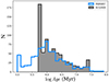 |
Fig. H.3. Distribution of all stellar ages from the final catalogue. The black histogram filled with grey shows ages estimated based on evolutionary tracks from Baraffe et al. (2015) and Siess et al. (2000), while the open blue histogram shows stellar ages based on PARSEC models (Bressan et al. 2012). PARSEC models span ages down to 0.1 Myr, while the other two go to 0.5 Myr. Both histograms have the same bins fixed to the distribution of PARSEC ages. |
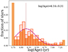 |
Fig. H.4. Fraction of stellar ages derived from HR diagram for stars with log(Teff) < 3.73, analogous to Fig. 10 but using tracks from Baraffe et al. (2015) and Siess et al. (2000). The filled orange histogram shows distribution for the whole sample, while the hatched red histogram represents the fraction distribution after removing the extreme bars with respect to the total number of stars within the new age range. The normal fit to the probability density distribution converted into the fraction distribution for the visual purposes is shown as a dark violet curve with a mean value of log(age) = 6.16 ± 0.31, corresponding to 1.4 |

We chose PARSEC models for the analysis because they allow homogeneous treatment of all stars in our sample, spanning a wide range of masses. We note however that individual estimates of stellar parameters are uncertain by an unknown value. The short comparison here between two sets of tracks shows that values of both masses and ages can differ by a factor of a few depending on the chosen tracks. This significantly exceeds any possible estimates of errors of those parameters done, accounting for observational uncertainties and the tabulation of spectral templates used here. Therefore, in Tables 1 and D.1 we only report estimated values, as true uncertainties are impossible to assess.
Appendix I: Young stars in Trumpler 14
Here, we complete the discussion in Section 4.3 showing the distribution of NIR excess and X-ray sources on the CMD (Fig. I.1) and the sky (Fig. I.2). To define NIR excess stars, we collected the NIR photometry from Preibisch et al. (2011a) and Preibisch et al. (2014), and followed the definition of the NIR excess of Zeidler et al. (2016). Whenever photometry from both catalogues was available, we chose the one with a better S/N. X-ray detections originate in the Chandra Carina Complex Project (CCCP, Townsley et al. 2011). NIR excess is often interpreted as a signpost of the inner circumstellar disc, while strong X-ray emission is expected from low-mass stars. The distributions of both characteristics confirm that the core of Tr 14 consists mainly of young stars (∼1 Myr), while the extended, halo population has more diverse ages, including very young stars. There is no strong correlation between any of those characteristics and the location in the cluster of stars from the extended population.
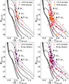 |
Fig. I.1. Colour-magnitude diagrams for de-reddened R and I band magnitudes from MUSE. Red hexagons mark stars within the core of Tr 14 (left, 0.9′, Kharchenko et al. 2013) or outside (right). The orange diamonds (top) indicate the NIR excess stars, while the dark blue crosses mark sources with a detected X-ray component (bottom, Townsley et al. 2011). |
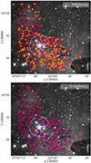 |
Fig. I.2. Locations of the NIR excess stars (orange diamonds, top) and the X-ray detections in Tr 14 (dark blue crosses, bottom). All stars studied here are marked with red dots, as in Fig. 1. The dashed circle with a radius of 0.9′ shows the core of the Tr 14, as defined by Kharchenko et al. (2013). The background image in grey-scale is the H-band image from HAWK-I (Preibisch et al. 2011a,b). |
All Tables
Parameters of stars removed from the catalogue due to the high background variation.
All Figures
|
Fig. 1. Trumpler 14 cluster studied in this work. Grey sky image from HAWK-I H-band observations (Preibisch et al. 2011a,b) shows the whole region, with the light grey grid of MUSE pointings and stars studied in this work marked as red circles. The five panels above and on the right show selected MUSE I band images. The panel inside consists of a mosaic of four MUSE pointing of the Tr 14 centre. Their numbers are indicated in the panels. Positions of the stars on MUSE images are marked with empty grey circles. The bar on the lower right corner of the HAWK-I image indicates the projected distance of 0.5 pc at the assumed distance of 2.35 kpc towards Tr 14 (Göppl & Preibisch 2022). |
| In the text | |
|
Fig. 2. Distribution of J-band magnitudes from HAWK-I in the MUSE field (Preibisch et al. 2011a,b). The dark berry-coloured histogram shows all HAWK-I measurements taken in the same area that was covered by MUSE. The violet distribution presents point source detections from Sect. 2.2.6, (upper panel) and in combination with the one excluded due to the high background variation and foreground stars (lower panel). In both panels, the grey line shows the completeness of our catalogue, defined as a ratio of the number of stars in a given magnitude bin (0.5 mag wide) in our catalogue and in the HAWK-I catalogue. |
| In the text | |
|
Fig. 3. Distribution of corrected parallaxes (light blue histograms) with a fitted normal distribution (purple line). Dash-dotted lines mark the 1σ width of the fitted distribution and applied ranges for excluding foreground and background stars. |
| In the text | |
|
Fig. 4. Colour–magnitude diagrams from MUSE broadband filters images in V and I (right panel), R and I magnitudes (middle panel), and I and J magnitudes (left panel). J band magnitudes are from VISTA and HAWK-I instruments. Shown are only data points with I band magnitudes above 3σ. Solid lines show PARSEC isochrones from 0.2 to 20 Myr and ZAMS, dotted lines show isomasses of 0.3, 0.7, 1, and 3 M⊙, as labeled (Bressan et al. 2012). Isochrones were reddened by the average extinction AV = 2.6 mag measured from MUSE spectra (see Sect. 3.4). Additionally, we plot the ZAMS reddened by AV = 1.4 mag with grey lines. |
| In the text | |
|
Fig. 5. Example of a MUSE spectrum (solid red line) of an M-type star and the matching spectral template (dashed black line). Both spectra are normalised at 7500 Å. |
| In the text | |
|
Fig. 6. Example of the MUSE spectrum (solid red line) of the K-type star and matching spectral template (dashed black line). Both spectra are normalised at 7500 Å. |
| In the text | |
|
Fig. 7. Distribution of AV estimated for Tr 14 stars. Additionally, we fitted the Gaussian function to estimate the centroid of the distribution. The centroid, the width of the distribution, and the median value in our sample are indicated in the upper right part of the figure. |
| In the text | |
|
Fig. 8. Colour–magnitude diagrams from MUSE broadband filters images in V and I (left panel), R and I magnitudes (middle panel), and I and J magnitudes (right panel) corrected for individual extinction. J-band magnitudes are from the VISTA and HAWK-I observations. Reddening vectors in the lower left corners show reddening by a median value of AV estimated for Tr 14. Solid lines show isochrones from 0.2 to 20 Myr (and ZAMS); dotted lines show isomasses of 0.3, 0.7, 1, and 3 M⊙, as labeled (Bressan et al. 2012). |
| In the text | |
|
Fig. 9. HR diagram for low-mass stars of Tr 14. Filled circles show data points. Empty squares are the median values of the bolometric luminosity for each spectral subclass, with error bars indicating 1-σ percentiles. Theoretical tracks from Bressan et al. (2012) are shown as solid black lines. Dotted grey lines show tracks for 0.3, 0.7, 1, and 3 M⊙ stars. |
| In the text | |
|
Fig. 10. Fraction of stellar ages derived from HR diagram for stars with log(Teff) < 3.73. The filled orange histogram shows the distribution of the whole sample, while the hatched red histogram represents the fraction distribution after removing the extreme bars with respect to the total number of stars within the new age range. The normal fit to the probability density distribution converted into the fraction distribution for the visual purposes is shown as a dark violet curve with a mean value of log(age) = 5.96 ± 0.41, corresponding to the 0.9 |
| In the text | |
|
Fig. 11. Locations of the Li 6708 Å detections in the MUSE field (blue crosses). All the stars studied here are marked with red dots, as in Fig. 1. The dashed circle with a radius of 0.9′ shows the core of Tr 14, as defined by Kharchenko et al. (2013). The background image in grey-scale is the H-band image from HAWK-I (Preibisch et al. 2011a,b). |
| In the text | |
|
Fig. 12. Colour-magnitude diagrams for de-reddened R and I band magnitudes from MUSE. Red hexagons mark the stars within the core of Tr 14 (left, 0.9′, Kharchenko et al. 2013) or outside (right). The blue crosses indicate the location of the lithium-bearing stars on the CMDs within and outside the core radius, respectively. The same tracks are plotted as in Fig. 8. |
| In the text | |
|
Fig. 13. Distribution of stellar masses in Tr 14 for stars with log(Teff) < 3.73. Top: filled histograms present the distribution of the masses of stars analysed in this paper. On top of it (hatched histogram) we display the distribution of the probable members with uncertain photometry removed from the analysis due to the high variability of the background emission. As is expected, most of the removed stars are faint, low-mass objects. Bottom: fraction of stars in the final spectroscopic catalogue within each mass bin relative to the combined catalogues of the final sample and probable members with uncertain photometry due to the variable background emission. The bins are the same as in the upper panel. |
| In the text | |
|
Fig. B.1. Distribution of differences in right ascensions and declinations from MUSE and Gaia DR3 at each field. |
| In the text | |
|
Fig. B.2. Separations in arcsec between MUSE and Gaia DR3 stars on a logarithmic scale. The MUSE catalogue here contains data points as of Sec. 2.2.1, before removing uncertain photometry. Overplotted is the threshold separation of 0.5″ used in this work. |
| In the text | |
|
Fig. B.3. Proper motions of Gaia counterparts. We show points with available proper motion measurements (grey dots) and with good astrometry (dark blue circles) (see Sec. 2.2.6 for details). Uncertainties of the latter points are smaller than the symbol sizes. Foreground and possibly contaminated stars are excluded. For reference, we also mark group proper motions from Berlanas et al. (2023) derived from Gaia EDR3 astrometry of OB stars in Tr 14. |
| In the text | |
|
Fig. C.1. Examples of spectra observed twice. Spectra were normalised to the flux at 7500 Å. The label indicates the source identifier and its S/N of around 7500 Å which was used to decide which spectrum to keep for the analysis. |
| In the text | |
|
Fig. D.1. Left: Distribution of the number of sources within a separation of 20″ from a given star. Right: Distribution of the STD of background emission estimated in the I band from the individual measurements within 20″ of the given star. |
| In the text | |
|
Fig. E.1. Difference between MUSE and WFI (Beccari et al. 2015) I band photometry as a function of MUSE colour R − I. Every panel represents a separate field, as indicated in the upper right corner. The dashed grey line shows the mean difference between I band magnitudes applied to MUSE photometry as magnitude correction. |
| In the text | |
|
Fig. E.2. Distribution of corrected MUSE magnitudes. colours indicate different photometric bands as stated in the upper left corner of the figure. Dashed lines show the turn-over point of the distributions located at: 18.01 mag (I band), 17.60 mag (R band), 17.58 mag (V band). |
| In the text | |
|
Fig. G.1. The |
| In the text | |
|
Fig. G.1. (cont.) The |
| In the text | |
|
Fig. G.3. The |
| In the text | |
|
Fig. H.1. HR diagram for low-mass stars of Tr 14. Empty circles show data points. Open squares are median values of the bolometric luminosity for each spectral subclass, with error bars indicating 1-σ percentiles. Theoretical tracks from Baraffe et al. (2015) are shown as solid grey lines, whereas tracks from Siess et al. (2000) are plotted as dashed lines. Dotted lines show tracks for various masses of stars. |
| In the text | |
|
Fig. H.2. Distribution of all stellar masses from the final catalogue on a logarithmic scale. The black histogram filled with grey shows masses estimated based on evolutionary tracks from Baraffe et al. (2015) and Siess et al. (2000), while the open blue histogram shows stellar masses based on PARSEC models (Bressan et al. 2012). |
| In the text | |
|
Fig. H.3. Distribution of all stellar ages from the final catalogue. The black histogram filled with grey shows ages estimated based on evolutionary tracks from Baraffe et al. (2015) and Siess et al. (2000), while the open blue histogram shows stellar ages based on PARSEC models (Bressan et al. 2012). PARSEC models span ages down to 0.1 Myr, while the other two go to 0.5 Myr. Both histograms have the same bins fixed to the distribution of PARSEC ages. |
| In the text | |
|
Fig. H.4. Fraction of stellar ages derived from HR diagram for stars with log(Teff) < 3.73, analogous to Fig. 10 but using tracks from Baraffe et al. (2015) and Siess et al. (2000). The filled orange histogram shows distribution for the whole sample, while the hatched red histogram represents the fraction distribution after removing the extreme bars with respect to the total number of stars within the new age range. The normal fit to the probability density distribution converted into the fraction distribution for the visual purposes is shown as a dark violet curve with a mean value of log(age) = 6.16 ± 0.31, corresponding to 1.4 |
| In the text | |
|
Fig. I.1. Colour-magnitude diagrams for de-reddened R and I band magnitudes from MUSE. Red hexagons mark stars within the core of Tr 14 (left, 0.9′, Kharchenko et al. 2013) or outside (right). The orange diamonds (top) indicate the NIR excess stars, while the dark blue crosses mark sources with a detected X-ray component (bottom, Townsley et al. 2011). |
| In the text | |
|
Fig. I.2. Locations of the NIR excess stars (orange diamonds, top) and the X-ray detections in Tr 14 (dark blue crosses, bottom). All stars studied here are marked with red dots, as in Fig. 1. The dashed circle with a radius of 0.9′ shows the core of the Tr 14, as defined by Kharchenko et al. (2013). The background image in grey-scale is the H-band image from HAWK-I (Preibisch et al. 2011a,b). |
| In the text | |
Current usage metrics show cumulative count of Article Views (full-text article views including HTML views, PDF and ePub downloads, according to the available data) and Abstracts Views on Vision4Press platform.
Data correspond to usage on the plateform after 2015. The current usage metrics is available 48-96 hours after online publication and is updated daily on week days.
Initial download of the metrics may take a while.