| Issue |
A&A
Volume 685, May 2024
|
|
|---|---|---|
| Article Number | A126 | |
| Number of page(s) | 42 | |
| Section | Interstellar and circumstellar matter | |
| DOI | https://doi.org/10.1051/0004-6361/202346465 | |
| Published online | 16 May 2024 | |
PRODIGE – planet-forming disks in Taurus with NOEMA
I. Overview and first results for 12CO, 13CO, and C18O
1
Max-Planck-Institut für Astronomie (MPIA),
Königstuhl 17,
69117
Heidelberg,
Germany
e-mail: This email address is being protected from spambots. You need JavaScript enabled to view it.
2
Department of Chemistry, Ludwig-Maximilians-Universität,
Butenandtstr. 5–13,
81377
München,
Germany
3
LAB, Université de Bordeaux,
B18N, Allée Geoffroy Saint-Hilaire, CS 50023,
33615
Pessac Cedex,
France
4
CNRS, Université de Bordeaux,
B18N, Allée Geoffroy Saint-Hilaire, CS 50023,
33615
Pessac Cedex,
France
5
IRAM,
300 Rue de la Piscine,
38046
Saint-Martin-d’Hères,
France
6
Max-Planck-Institut für extraterrestrische Physik (MPE),
Gießenbachstr. 1,
85741
Garching bei München,
Germany
7
IPAG, Université Grenoble Alpes, CNRS,
38000
Grenoble,
France
8
Centro de Astrobiología (CAB), CSIC-INTA,
Ctra Ajalvir Km 4, Torrejón de Ardoz,
28850
Madrid,
Spain
9
Department of Astronomy, The University of Texas at Austin,
2500 Speedway,
Austin,
TX
78712,
USA
10
I. Physikalisches Institut, Universität zu Köln,
Zülpicher Str. 77,
50937
Köln,
Germany
Received:
20
March
2023
Accepted:
22
February
2024
Abstract
Context. The physics and chemistry of planet-forming disks are far from being fully understood. To make further progress, both broad line surveys and observations of individual tracers in a statistically significant number of disks are required.
Aims. Our aim is to perform a line survey of eight planet-forming Class II disks in Taurus with the IRAM NOrthern Extended Millimeter Array (NOEMA), as a part of the MPG-IRAM Observatory Program PRODIGE (PROtostars and DIsks: Global Evolution; PIs: P. Caselli and Th. Henning).
Methods. Compact and extended disks around T Tauri stars CI, CY, DG, DL, DM, DN, IQ Tau, and UZ Tau E are observed in ~80 lines from > 20 C-, O,- N-, and S-bearing species. The observations in four spectral settings at 210–280 GHz with a 1σ rms sensitivity of ~8–12 mJy beam−1 at a 0.9″ and 0.3 km s−1 resolution will be completed in 2024. The uv visibilities are fitted with the DiskFit model to obtain key stellar and disk properties.
Results. In this first paper, the combined 12CO, 13CO, and C18O J = 2–1 data are presented. We find that the CO fluxes and disk masses inferred from dust continuum tentatively correlate with the CO emission sizes. We constrained dynamical stellar masses, geometries, temperatures, the CO column densities, and gas masses for each disk. The best-fit temperatures at 100 au are ~ 17–37 K, and decrease radially with the power-law exponent q ~ 0.05–0.76. The inferred CO column densities decrease radially with the power-law exponent p ~ 0.2–3.1. The gas masses estimated from 13CO (2–1) are ~0.001–0.2 M⊙.
Conclusions. Using NOEMA, we confirm the presence of temperature gradients in our disk sample. The best-fit CO column densities point to severe CO freeze-out in these disks. The DL Tau disk is an outlier, and has either stronger CO depletion or lower gas mass than the rest of the sample. The CO isotopologue ratios are roughly consistent with the observed values in disks and the low-mass star-forming regions. The high 13CO/C18O ratio of ~23 in DM Tau could be indicative of strong selective photodissociation of C18O in this disk.
Key words: line: profiles / techniques: interferometric / protoplanetary disks / stars: variables: T Tauri, Herbig Ae/Be / radio lines: planetary systems
NSF Astronomy and Astrophysics Postdoctoral Fellow.
© The Authors 2024
 Open Access article, published by EDP Sciences, under the terms of the Creative Commons Attribution License (https://creativecommons.org/licenses/by/4.0), which permits unrestricted use, distribution, and reproduction in any medium, provided the original work is properly cited.
This article is published in open access under the Subscribe to Open model.
Open access funding provided by Max Planck Society.
1 Introduction
A diversity of discovered exoplanets calls for abetter understanding of the physical and chemical processes in their natal planet-forming disks (e.g., Mordasini et al. 2012; Turrini et al. 2021; Mollière et al. 2022). Recently, young planets have been imaged inside the gas-rich PDS 70 disk for the first time (e.g., Keppler et al. 2018; Haffert et al. 2019; Facchini et al. 2021). However, despite extensive progress achieved with the powerful Very Large Telescope (VLT), Spitzer, James Webb Space Telescope (JWST), Herschel, Atacama Large Millimeter/Submillimeter Array (ALMA), extended Jansky Very Large Array (eVLA), and NOrthern Extended Millimeter Array (NOEMA), our understanding of the disk physics and chemical composition is still limited. Among the key disk properties, we have only begun to determine their (1) mass measurements, (2) dust-to-gas ratios, (3) temperature structures, and (4) elemental ratios and molecular abundances in the gas and ice phases (e.g., Andrews 2020; Öberg et al. 2021; Benisty et al. 2023; Manara et al. 2023; Miotello et al. 2023; Öberg et al. 2023).
The majority of the disk masses have been inferred from the dust continuum data, often by using fixed dust emissivities and/or dust temperatures, and ill-constrained gas-to-dust ratios (see, e.g., Bergin & Williams 2018; Manara et al. 2023, and references therein). Gas masses in a limited number of disks have been obtained by more direct methods. By observing HD emission with Herschel and performing disk temperature modeling, the gas masses of TW Hya, DM Tau, and GM Aur disks have been directly inferred (Bergin et al. 2013; McClure et al. 2016; Trapman et al. 2017). Using CO emission observed with ALMA, Lodato et al. (2023) have constrained the self-gravity of the IM Lup and GM Aur disks, and derived gas masses of ~0.1 M⊙ and ~0.26 M⊙, respectively. Yoshida et al. (2022) have measured the pressure broadening of the 12CO (3−2) line and inferred high gas densities in the inner TW Hya disk midplane. Modeling the dust emission sizes at multiple wavelengths has also provided constraints on the gas surface densities, suggesting that the disks could be more massive than previously thought (Birnstiel et al. 2018; Powell et al. 2019; Trapman et al. 2020; Franceschi et al. 2022; Tazzari et al. 2021).
Disk temperatures at distinct vertical layers are usually probed via a combination of the optically thick and thin lines, such as CO, and they often show the presence of radial and vertical gradients (e.g., Dartois et al. 2003; Williams & Best 2014; Cleeves et al. 2016; Miotello et al. 2018, 2023; Teague et al. 2018b; Calahan et al. 2021b,a; Schwarz et al. 2021). For edge-on or well-resolved disks, the vertical temperature profile can be derived directly from the line observations (e.g., Dutrey et al. 2017; Pinte et al. 2018; Law et al. 2021b; Paneque-Carreño et al. 2022). Such studies require combined physical, chemical, and radiative transfer modeling, and hence considerable effort to reach a balance between the model feasibility and its computational costs (Haworth et al. 2016).
In addition to temperatures, turbulent properties of the gas in disks can be estimated from the high signal-to-noise ratio (S/N) line data by accounting for the Keplerian shear and thermal broadening, which requires a good understanding of the underlying thermal structures (e.g., Guilloteau et al. 2012; Teague et al. 2016; Flaherty et al. 2020; Paneque-Carreño et al. 2023). Subsonic turbulence has only been firmly detected in the DM Tau and IM Lup disks so far. The deviations from Keplerian rotation have been found in various disks, which could be signatures of embedded planets or disk winds (e.g., Teague et al. 2018a, 2021; Pinte et al. 2019; Boehler et al. 2021; Stadler et al. 2023).
To better understand the cause of the apparent lack of turbulence in disks, studies of disk ionization are important. Usually, the combination of the HCO+ and N2H+ isotopologues are used to probe the disk ionization degree, which is driven by the interstellar or stellar X-rays and cosmic ray particles (Dutrey et al. 2007; Öberg et al. 2011; Cleeves et al. 2015; Teague et al. 2015; Aikawa et al. 2021). The impact of the impinging stellar far-ultraviolet (FUV) radiation on disk properties and molecular composition can be characterized via observations of FUV tracers such as C2H, c-C3H2, CN, HCN, and HNC, combined with disk chemistry models (e.g., Bergin et al. 2003; Henning et al. 2010; Chapillon et al. 2012; Guzmán et al. 2015; Bergner et al. 2021).
The inferred abundances of CO isotopologues, light hydrocarbons (e.g., C2H), and sulfur-bearing species have revealed substantial depletion of the elemental sulfur and oxygen in some disks, and the nonsolar elemental C/O ratios in their molecular layers (e.g., Bergin et al. 2016; Kama et al. 2016; Semenov et al. 2018; Le Gal et al. 2019; Miotello et al. 2019; Fedele & Favre 2020; Rivière-Marichalar et al. 2020; Bosman et al. 2021; Cleeves et al. 2021; Le Gal et al. 2021; Phuong et al. 2021; Ruaud et al. 2022; Anderson et al. 2022; Furuya et al. 2022a; Pascucci et al. 2023). A possible reason for the excessive volatile depletion in the disk molecular layers is the chemical processing and sequestration into refractory ices, which sediment toward the disk midplanes along with the growing dust grains (Favre et al. 2013; Öberg & Bergin 2016; Krijt et al. 2020; Eistrup & Henning 2022; Van Clepper et al. 2022). Still, the overall chemical composition and partitioning of the elemental C, O, N, and S into various species remain poorly constrained in disks. Therefore, a homogeneous study of the disk composition in many chemical species is necessary, and to begin with we need the high S/N CO isotopologue data.
Last but not least, ubiquitous ~1–100 au substructures, such as inner holes, gaps, rings, spirals visible in both the gas and dust emission are indicative of the planet formation, planet-disk interactions, or disk instabilities, which further complicates the analysis and interpretation of the observations (e.g., ALMA Partnership et al. 2015; Long et al. 2017; Andrews et al. 2018; Smirnov-Pinchukov et al. 2020; Law et al. 2021a; Bae et al. 2023; Jennings et al. 2022; Zhang et al. 2023). The “Molecules with ALMA at Planet-forming Scales” (MAPS) collaboration has performed the high-resolution, multiband ALMA observations of the IM Lup, GM Aur, AS 209, HD 163296, and MWC 480 disks down to the ~10–20 au scales (Öberg et al. 2021, and references therein). The MAPS team has found a variety of small-scale dust and chemical substructures in these disks, characterized their molecular complexity and the C/O ratios, and revealed complex disk dynamics suggestive of the planet-disk interactions and disk winds.
With the goal of better constraining the physical and chemical structures in the Class 0/I and Class II sources, we have conceived the MPG-IRAM large observing project PRODIGE (PROtostars to Disks: Global Evolution) at NOEMA. The first studies of the Class 0/I protostars in Perseus have been published in Valdivia-Mena et al. (2022) and Hsieh et al. (2023). Here, we present the first paper about Class II disks in Taurus. This paper focuses on the analysis and modeling of the CO isotopologue data to unveil the geometry, physical structure, and CO depletion of the targeted disks, which are needed for the future analysis and modeling of other emission lines. The overview of the project, its scientific goals, and sample selection are described in Sect. 2. The observations and CO line data are presented in Sects. 3 and 4, respectively. The results of the parametric fitting and empirical trends between various disk and stellar parameters are presented and discussed in Sect. 5. Our summary and conclusions are provided thereafter.
2 PRODIGE overview, scientific goals, and sample
The recently upgraded NOEMA interferometer with 12 × 15-m antennas operating at 70–280 GHz with up to ~1800 m long baselines is a powerful facility1 (see Schuster et al., in prep.). The PolyFiX correlator can be tuned to include up to 64 × 62.5 kHz spectral windows in dual polarization, or used with a uniform 250 kHz resolution across the full 15.5 GHz bandwidth (Gentaz 2019). In the high-resolution mode, one can target four times more molecular lines compared to the ALMA correlator, which makes NOEMA on par with ALMA for the line surveys at ~0.5–1″ resolution.
In light of these considerations, we have devised the large program PRODIGE at NOEMA to study in a coherent manner the physics and chemistry at ~ 100 au scales in 8 protoplanetary disks in Taurus (PI: Th. Henning; 260 h) and in 30 low-mass protostars in Perseus (PI: P. Caselli; 260 h). The observations began in 2020 and will be completed in 2024. Below we describe the science goals, the sample, and the strategy of the Class II disk part of the PRODIGE project.
Stellar properties.
2.1 Sample
In contrast to the MAPS project that has targeted 2 T Tauri and 3 Herbig Ae disks from various star-forming regions (SFRs) (Öberg et al. 2021), we decided to focus on both the large (>300 au) and compact (< 300 au) T Tauri disks in Taurus SFR. We chose the T Tauri systems with the stellar masses of M* ≲ 1 M⊙, outside the ~1.1–2.1 M⊙ mass range targeted in the MAPS project (Öberg et al. 2021). By focusing on the disks that have been formed in the same star-forming region from similar initial conditions, we are able to perform a less biased comparison of the disk properties between the sources (Ansdell et al. 2018; Luhman 2018; Miotello et al. 2023).
The Taurus SFR is young, ~1–5 Myr (Luhman 2023), nearby (~140–170 pc; Gaia Collaboration 2018), and has solar-like metallicities (Cartledge et al. 2006; D’Orazi et al. 2011; Nieva & Przybilla 2012), which together with a large, >200 population of Class II disks (Esplin & Luhman 2019) and a lack of massive stars make it an attractive environment to study the evolution of protoplanetary disks.
To optimize the available observing time at NOEMA, we decided to target a limited number of sources but with a high enough sensitivity to detect as many weak lines of multiple species as possible. Our sample selection criteria were: 1) Class II sources in Taurus with ages of ~1–5 Myr, 2) isolated stars without severe foreground extinction (AV < 3 mag), 3) T Tauri stars only, M* ~ 0.4–1.0 M⊙, 4) compact and extended disks without severe substructures visible in the ALMA continuum images (Long et al. 2018, 2019), 5) disks with 1.3 mm continuum fluxes of >60 mJy to allow self-calibration, 6) disks with previous molecular line detections (Guilloteau et al. 2016), and 7) at least one disk with measured gas mass via the HD lines.
Thus, we have selected the following eight systems:
DM Tau: a large, moderately inclined disk (~35°) with a gas mass measured via the HD emission with Herschel (Piétu et al. 2007; McClure et al. 2016);
DL Tau, CI Tau, CY Tau, IQ Tau, DN Tau: less extended disks with inclinations up to 55° (Guilloteau et al. 2011; Long et al. 2018);
UZ Tau E: a compact, circumbinary disk with a small inner hole and an inclination of ~56° (Long et al. 2018);
DG Tau: a Class I/II object with a jet and an outflow, and an inclination of ~32° (perhaps, part of a wide binary system with DG Tau B; Guilloteau et al. 2011).
Only some of the targeted disks have been observed with ALMA in the CO isotopologue lines with the sensitivity and resolution comparable to our PRODIGE NOEMA survey (in particular, C18O). Furthermore, CY Tau, DM Tau, DL Tau, DN Tau, and DG Tau have been observed with JWST in Cycle 1 in the framework of the GTO program “MIRI EC Protoplanetary and Debris Disks Survey” (GTO 1282; PI: Th. Henning2).
The basic properties of our disk sample are summarized in Tables 1 and 2. The additional information about individual sources can be found in Appendix A.
2.2 Main science goals
In this first paper, we aim to derive the disk temperature and density structures, using the optically thick and thin CO isotopologue data, and the power-law radiative transfer model DiskFit (e.g., Piétu et al. 2007). The best-fit radial temperature and column density profiles that are presented in this paper were also utilized as priors to reconstruct 1+1D radial and vertical disk structures using the physical, chemical and line radiative transfer model DiskCheF (presented in Franceschi et al. 2024).
In the next study, we aim to constrain the disk ionization from a combination of the optically thick and thin HCO+ (3−2) and N2H+ (3−2) isotopologue lines, using the best-fit disk physical structures obtained from the CO data. The disk turbulence (or the upper limits) will be constrained from the CS data to minimize the thermal broadening contribution to the local line profiles.
After that, using the reconstructed best-fit physical structures and a variety of detected molecules, the CHNOS chemistry, the volatile budget, and the presence of the large-scale radial chemical substructures in the disk sample will be studied. We will infer the gas-phase elemental ratios and depletion factors, and will investigate the impact of the high-energy FUV and X-ray radiation on disk chemistry from the combination of C2H, CN, HCN, and HNC. The efficiency of the D-, 13C-, and 18O-fractionation will be inferred from the analysis of the observed ratios of DCN/HCN, DNC/HNC, N2D+/N2H+, etc., coupled with the chemical model with fractionation processes. The inferred chemical abundances, elemental ratios, depletion factors and isotopic ratios will be correlated with the key stellar and disk physical quantities (mass, size, gas temperature, etc.).
Disk properties.
3 Observations and methods
We observed the GO Tau disk in a pilot 1 mm line survey with NOEMA, using 9 antennas in C configuration (~0.9″ beam), reaching the sensitivity of 8–12 mJy beam−1 at 0.3 km s−1 resolution after ~4–6 h of the on-source integration (Guilloteau et al., in prep.). This combination between the resolution and integration time allowed us detecting and at least partially resolving the line emission from key CHONS species and their isotopologues, and is optimal for the line surveys in nearby protoplanetary disks. The four PolyFiX spectral settings in the 210–280 GHz range with a total 62 GHz coverage were required to target the majority of the detected or potentially detectable molecular transitions. We employed the same observing strategy for the PRODIGE project, where each disk is observed for 4–6 h using the same spectral setup and antenna configuration each year (four different spectral setups between 2020 and 2024).
3.1 PolyFiX/NOEMA observations
Observations of the eight T Tau disks were carried out at the NOEMA interferometer with the PolyFiX correlator in Band 3 (1.3 mm) between 2020, January 9 and 2020, November 30 (project L19ME; PI: Thomas Henning, co-PI P. Caselli and S19AW for DN Tau and CI Tau). We used high-resolution, 62.5kHz spectral chunks to target specific emission lines over the ~15.5 GHz PolyFiX bandwidth in dual polarization (other spectral windows had a 2 MHz resolution). The first observing run covered the main CO isotopologues in order to better characterize the disk physics, which is needed for the further analysis and chemical modeling. In addition to 12CO, 13CO, C18O and 13C17O (2−1), the lines of para-H2CO, DCO+, DCN, DNC, 13CN, cyclic C3H2, C2D, HC3N, N2D+, and other rare species were targeted. The spectral setup was centered at ~225 GHz and covered, in total, ~40 molecular lines in 27 high resolution spectral windows. The spectral setup is shown in Fig. B.1 and targeted molecular lines and their spectroscopic parameters are listed in Table B.1. In 2021–2023, two other spectral setups were observed, covering CN, 13CN, cyclic C3H2, ortho-H2CO, HCN isotopologues and HCO+ isotopologues, CS, H2CO, and other species, respectively (the data will be presented in a future paper).
Observations were carried out with ten antennas in the C configuration. Each source was observed independently (no track-sharing) with one to three tracks, using the quasars J0438+300 and 0507+179 as phase calibrators. 3C84 was the bandpass calibrator in all the tracks but the last one on UZ Tau E, where 3C454.3 was used instead. To ensure good relative flux calibration, LkHa 101 served as a flux calibrator in all datasets but one on UZ Tau E (this last track was calibrated using the common calibrator with the first track observed on this source the day before). MWC349 and 2010+723 have been additional flux calibrators on some tracks (for more detail, see Table B.2). Absolute flux calibration uncertainties for our CO data are within 10% or better. Mean on-source integration time was 5.5 h per source. The 1σ rms noise varies from source to source and is 3.7–9.2 mJy at 0.3 km s−1 resolution.
3.2 Data reduction
The raw data were reduced and calibrated at IRAM, using GILDAS/CLIC package (version 24sep19 02:05 cest)3. For each track, we ran the CLIC reduction pipeline and, based on the astronomer on duty’s notes and after data inspection, corrected for failures (via flagging) or inaccurate baseline measurements (using measurements taken after the original observation). The calibrator fluxes (and their time variations) were bootstrapped and applied to each dataset through a final round of amplitude calibration. The uv tables were generated at full spectral resolution for each source and spectral window.
3.3 Line imaging
Self-calibration and imaging were performed with the Imager software4, using an automatic pipeline, a custom-built line catalog, and third-party Python tools. Before any processing, we accounted for the source proper motions by using the Gaia DR2 measurements and the UV_PROPER_MOTION command on each UV table. After self-calibration, the solutions were applied to the line spectra in the respective sidebands to improve their S/N. To increase the S/N, the line data were resampled to 0.3 km s−1 spectral resolution before imaging and deconvolution. To further maximize the sensitivity, the data were cleaned using natural weighting with the Hogbom algorithm. After that, channel and moment maps were created. The synthesized beams are ≈1.1–1.5″ × 0.5–0.7″, for the major and minor beam axis, respectively. The corresponding positional angles are ~15–20°. Even in the worst case, the beam major axis is at most at 45° from the disk minor axis, making the disks properly spatially resolved.
To further increase the S/N of the data, we used the Kepler pixel deprojection technique presented in Teague et al. (2016); Yen et al. (2016); Matrà et al. (2017). This technique allows shifting and stacking individual spectra by taking the disk geometry, distance and Keplerian velocities into account, boosting the S/N for detected emission. It also allows recovering the emission radial profile. We use the implementation available through the KEPLER command in the Imager package. It is similar to that available through the GoFish5 tool (Teague 2019). The Imager implementation provides the radial brightness profile distribution by slicing the data into radial bins, and for each bin, computing the average spectrum over azimuth, thereby producing a Radius-Velocity diagram. The radial profile is obtained by retaining the maximum brightness found as a function of velocity, and an error estimate is derived from the spectra. This peak brightness estimator is more reliable than the line integrated flux, as faint line wings are always difficult to properly fit to derive such flux accurately. However, in the inner part of disk, which remains spatially unresolved, the peak brightness is reduced compared to the intrinsic source brightness due to beam dilution. The method works well because geometrical parameters (including the projected Keplerian velocities) are well defined from the bright lines such as 12CO (2−1). The only exception was DG Tau due to its complex structure and the presence of the outflow and shocks, hence only the standard line imaging was done for this source.
3.4 DiskFit model
The radiative transfer code DiskFit was used to fit the observed uv-visibilities (see e.g., Piétu et al. 2007). Rotationally symmetric disk structure was assumed, with power laws used to describe disk surface density, temperature, molecular column density radial profiles, etc. The disk was assumed to be vertically isothermal, with vertically uniform relative molecular abundances and Gaussian density distribution for the total gas density. The LTE excitation conditions have been assumed, and the ray tracing was used to calculate synthetic line emission. The observational data were fitted in Fourier space by the Levenberg–Marquardt χ2 minimization, using the same uv sampling in the model as in the observed data. The symmetric 1σ error bars that include thermal noise and phase calibration errors were obtained through the covariance matrix. This minimization method is sufficient despite the large number of model parameters (up to 17), because as discussed by Piétu et al. (2007), except for the rotation velocity-inclination pair coupled through v sin i, parameters are only weakly coupled as can be seen from the MCMC fitting done by Simon et al. (2017), their Fig. B11.
The validity of the power law assumptions in the DiskFit model relies on rapid decrease of the disk surface density with radius, the known Keplerian rotation pattern for the gas, and power-law-like radial decrease of the temperature as probed from the CO emission. As was discussed in Piétu et al. (2007) and Phuong et al. (2020), these are reasonable assumptions for outer, ≳50–100 au regions in low-mass, Class II T Tauri disks without severe substructures, as considered in the present study. In inner, ≲30–80 au disk regions, temperature distributions could become flatter, as was found, for example, by the modeling of the CO ALMA data from MAPS large program (Law et al. 2022).
While these assumptions apply reasonably well for at least CO and its isotopologues in the sample of disks studied here, the assumption of a power-law radial decrease in molecular column density for other species could be less justified due to the presence of chemical and/or excitation effects, which will be investigated in subsequent papers. The azimuthally averaged CO intensity profiles presented below do not show large-scale substructures. We have further tested applicability of the power-law DiskFit model for recovering the underlying disk physical parameters. For that, we have generated synthetic CO isotopologue datacubes with a 2D-line radiative transfer model URANIA, assuming a power-law surface density profile, hydrostatic equilibrium in vertical direction, thermal structure computed by radiative transfer, and using a full gas-grain chemistry, and found that the DiskFit model can recover the underlying disk properties well (Pavlyuchenkov et al. 2007).
To facilitate the fitting, we used the stellar masses and geometric parameters (position, inclination, orientation) from the previous studies and the CO data (see Tables 1–2). In a first iteration, a fit of the optically thick 12CO (2−1) line was used to determine the gas temperature, assuming it follows a power law distribution (Tk(r) = T0 × (r/100 au)−q). High enough 12CO column densities were assumed to ensure optical thickness of the synthetic 12CO (2−1) emission (e.g., N(CO) > 1016 cm−2 at 100 au). The temperature Tk(r) derived from fitting the optically thick 12CO line was used to fit mostly optically thin 13CO (2− 1) data and to determine the 13CO column density distribution (N(CO; r) = N0 × (r/100 au)−p). As an initial guess for the 13CO column densities, the inferred 12CO column densities scaled down by a factor of 70 were utilized. We then iterated between 12CO and 13CO data in order to optimize the fit results. Finally, to successfully fit the weakest C18O (2−1) emission, the stellar masses, geometric parameters, and temperature profiles had to be fixed, using the best-fit values derived from the 13CO fitting. The results of the modeling are presented below in Sect. 5.1.
4 Results
4.1 CO line images
We present the 12CO (2−1) moment map, channel maps, integrated spectrum, and Keplerian plot for the bright and large DM Tau disk in Figs. 1–2. These plots look overall similar for the other CO isotopologues and for the other disks (although, usually, with more noise and, in some cases, contamination by molecular cloud, see Appendix C). The 12CO channel map in Fig. 1 shows a “butterfly” pattern characteristic of rotating Keplerian disks. The DM Tau 12CO observations are not affected by the foreground cloud absorption, which is also true for DN Tau and IQ Tau (see Appendix C). In contrast, the optically thick emission lines in CI, CY, DG, DL Tau, and UZ Tau E are partially obscured at ~4–6 km s−1. This absorption leads to asymmetric emission distributions in the integrated intensity maps and skewed double-peaked integrated spectra. For example, the NW half of the CI Tau disk appears much less pronounced than its SE half on the CI Tau integrated intensity map (see Fig. C.1).
The Keplerian deprojection transforms the double-peaked 12CO (2−1) integrated spectrum of the DM Tau disk with a ~2 km s−1 FWHM width and a peak value of ~9.5 Jy into a single peaked spectrum with a FWHM width of ~0.5 km s−1 and a peak value of ~27.7 Jy (see Fig. 2, top panel). This single-peaked integrated spectrum is well-fitted by a single Gaussian. The “teardrop” pattern visible in the bottom right panel of Fig. 2 is a characteristic signature of molecular emission from a Keplerian disk (e.g., Teague et al. 2016). It is fully symmetric with respect to the systemic velocity of 6.05 km s−1. The high-velocity “halo” visible at the inner ≲100 au radii in the teardrop plot represents the CO emission from the innermost disk region with the strongest gradients of physical conditions. It falls within a single beam and hence suffers from beam smearing and dilution.
The radial profile of the 12CO (2−1) line brightness temperature depicted in red in left panel in Fig. 2 is derived from the best-fit disk model, while the magenta dashed line shows the expected brightness of a completely optically thick line. The overall agreement between these curves and the observed profile indicates that CO is mostly optically thick and that the power-law approximation for the temperature is appropriate at this scale. The line brightness temperature distribution has a skewed Gaussian-like profile, with an inner “hole” inside r ~ 150 au, followed by an extended bell-like peak with TB ~ 16 K, and a steady decline until r ~ 1000 au. The apparent drop within the inner r ≲ 150 au is a result of beam dilution. The radial extent of the 12CO (2−1) line brightness temperature of ~1000 au is larger than the CO gas radius estimate of ~900 ± 10 au (Table 2) due to our limited angular resolution.
The line brightness radial profiles look similar in the other disks and for the other CO isotopologue lines, and do not show any significant substructures. The targeted disks do not have prominent inner holes with sizes of ~50–100 au, neither in the dust nor gas distributions, and the ~100 au spatial resolution of our data does not permit us to infer the presence of smaller substructures in the disks. The typical peak TB values are ~6.5–16 K for 12CO (2−1), 1.2–7.5 K for 13CO (2−1), and 0.2–1.8 K for C18O (2−1), respectively. The ≈0.8–0.9″ beam (~100–150 au spatial scale) leads to the radially smooth TB(r) profiles, without any significant substructures visible in the plots. The emission radii vary from disk to disk and differ for each CO isotopologue, with the most extended emission in the 12CO (2−1) lines. As noted above, the inner “holes” with radii ≲100–150 au in the brightness temperature profiles are due to the beam dilution.
While the analysis of the large disk around DM Tau shows that the DiskFit modeling in terms of power laws is reasonably appropriate, the parameters derived from such models do start suffering from unavoidable degeneracy when the disk radius is small due to the limited angular resolution. For the smaller disks (DN Tau, IQ Tau and UZ Tau E), deriving both the column density and the temperature law becomes impossible as the optically thick core cannot be well separated from the optically thin outer part. The geometric parameters are, however, unaffected. Temperature can be derived from 12CO, while 13CO and C18O column densities can be derived assuming the same temperature as given from 12CO. Furthermore, in the relevant temperature range (20–30 K), the derived column densities are rather insensitive to the temperature. We provide below more specific details for each source.
CI Tau. Both the moment-zero map and the integrated spectrum of the 12CO (2−1) emission are affected by the foreground absorption at 4.2–6.5 km s−1 (Fig. C.1). It also causes the asymmetry of the teardrop plot and the slightly skewed deprojected integrated spectrum that cannot be fitted with a single Gaussian (Fig. C.2). The radial profile of the line brightness temperature is fainter than the best fit profile because of the absorption, and extends only up to ~600–650 au. In contrast, the 13CO and C18O (2−1) data unaffected by the cloud show smooth profiles and a broader extent of the line brightness temperature up to radius of ~900 au (Figs. C.3–C.6).
CY Tau. The 12CO (2−1) emission is also affected by the foreground absorption that is visible as stripes in the channel map at VLSR ~ 4.5 and 5 km s−1 (C.7). This is far from the systemic velocity of 7.3 km s−1, and thus both the moment-zero map and integrated spectrum are not strongly affected by the absorption. The asymmetry of the teardrop plot toward the red-shifted wing at radii ≲100 au is due to the cloud contamination (Fig. C.8). The CO emission for all isotopologues is compact, RCO ~ 300 au. Deriving a temperature profile from the CO data is ambiguous because of the combination of cloud contamination and relatively compact (RCO ~ 300 au) disk.
DG Tau. The 12CO (2−1) emission in the channel map reveals a complex structure, which consists of a large-scale envelope with filamentary structure, a bow shock at velocities of ~2.5–4 km s−1, and a Keplerian disk (Fig. C.13). The large-scale outflow emission is not directly visible on the 12CO (2−1) map, partly due to the lack of short spacing data. Strong foreground cloud and envelope absorption lead to the multiple absorption dips in the integrated spectrum. The same complex structure is present in more optically thin 13CO and C18O (2−1) emission maps (Figs. C.14–C.15). The C18O emission indicates a possible small (≲100 au radius) disk, but with no obvious signature for Keplerian rotation, given the weak S/N.
DL Tau. The 12CO (2−1) emission shows strong foreground absorption at VLSR ~ 5–6.5 km s−1, which is visible in the moment-0th map and integrated spectrum (Fig. C.16). Even more optically thin 13CO (2−1) emission is affected, and shows an arc-like integrated intensity distribution that is located offthe center (Fig. C.18, top right). The C18O (2−1) emission is weak and barely visible in the Keplerian deprojected plot (Fig. C.21). The CO line brightness temperatures are low in this disk, in particular for optically thin13CO and C18O (2−1) lines. The peak TB values are ~7.2 K for 12CO (2−1), ~1.3 K for 13CO (2−1), and only ~0.2 K for C18O (2−1), respectively. The observed 12CO (2−1) radial brightness profile differs from the fitted one because of cloud contamination around the systemic velocity. The 12CO (2−1) emission is clearly optically thick, and declines more steeply at the disk edge than for the minor CO isotopologues.
DM Tau. The 12CO (2−1) emission is not affected by the foreground absorption. The corresponding line brightness distribution TB(r) has an inner hole inside r ~ 130 au, followed by a peak brightness, and a 3-step decline until the radius of ~ 1 050 au, with the two turn-over points at r ~ 340 au and ~700 au, respectively (Fig. 2). The steeper profile between r ~ 800 au and ~1000 au could be caused by the tapered surface density distribution at the disk edge. The C18O (2−1) emission looks noisy because the DM Tau observations were done under suboptimal conditions during late April, leading to higher noise compared to the other disks in the sample (Fig. C.24).
DN Tau and IQ Tau. The CO isotopologue emission is compact, RCO ~ 200–300 au (Figs. C.26–C.37). The C18O (2−1) emission is weak. The IQ Tau disk shows low line brightness temperatures that are similar to those in the DL Tau disk. The peak TB temperatures are ~9.5 K for 12CO (2−1), ~1.2 K for 13CO (2−1), and only ~0.2 K for C18O (2−1), respectively. The FWHM widths of the CO deprojected spectra in the IQ Tau disk are ~1.5 km s−1. For DN Tau, the DiskFit analysis requires a central hole of 15–20 au (or substantially fainter emission within this radius) in all CO isotopologues to best represent the emission. An alternate solution is a rather flat temperature distribution (exponent q ≈ 0), which is less physically realistic. Both solutions result in a relative lack of emission at high velocities and can explain the faintness of the line wings.
UZ Tau E. The CO isotopologue emission maps show the presence of the prominent disk around the spectroscopic binary in the center, accompanied by the compact binary system UZ Tau W (Figs. C.38–C.43). Emission is also visible toward UZ Tau W in all CO isotopologues. The disk around UZ Tau E is clearly asymmetric in 12CO (2–1), with a tail of emission opposite to the position of the UZ Tau W binary. It extends to a similar distance as the apparent E–W star separation, clearly suggesting that all these stars were born in a common disk. The best-fit DiskFit analysis results in a compact CO disk with an outer radius of 200 au, which does not represent the extended emission at all. Moreover, there is a strong degeneracy between the assumed CO column density profile and the derived kinetic temperature profile, which is further influenced by the non-represented outer disk emission. High-temperature solutions (37 K at 100 au, with a steep exponent of −0.85) are possible for 12CO, but require lower column densities (<1017 cm−2) and relatively flat distribution with an exponent of 0.8. The emission from the minor CO isotopologues is more compact, with an outer radius around 140 au.
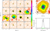 |
Fig. 1 Observations of 12CO (2−1) emission in the DM Tau disk. Shown are the channel map of the observed line brightness distribution (left), the moment-zero map (top right), and the integrated spectrum (bottom right). The channel map shows 16 velocity channels with a step of 0.5 km s−1 in the [−4.5, +4.5] km s−1 range around the systemic velocity. The contour lines start at 2 K, with a step of 2 K. The color bar shows line brightness temperatures (K). The contour lines in the moment-zero plot start at 3, 6, and 9σ, with a step of 6σ afterward. The 1σ rms noise (mJy km s−1) is shown in the upper left corner of the moment-zero plot, and the synthesized beam is depicted by the dark ellipse in the left bottom corner. |
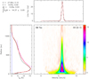 |
Fig. 2 Observations of 12CO (2−1) emission in the DM Tau disk. Shown is a pixel-deprojected Keplerian plot consisting of the three panels: (left) the radial profile of the line brightness temperature (K) with observations and errorbars in black, and profile derived from the best-fit disk model in red. The magenta dashed curve indicates the expected brightness temperature of an optically thick line derived from temperature power law. Top: the integrated spectrum (black line) overlaid with the best-fit Gaussian profile (red line). Bottom right: aligned and stacked line intensity (K) as a function of disk radius (Y-axis; au) and velocity (X-axis; km s−1). The color bar units are in kelvin. |
Parameters of the observed CO isotopologue lines.
4.2 Fluxes
The observed peak and integrated CO fluxes, along with the systemic velocities and the line widths, are presented in Table 3. The 1σ flux uncertainties were estimated from the rms noise in the emission-free channels. The system velocities have been derived with a precision of ≈4–100 m s−1 (with the uncertainties stemming from the Gaussian fit of the spectra). They vary between about 5.5 and 7.4 km s−1, depending on the source, which are typical values for the Taurus disks. The line widths corrected for the disk orientation, but not for Keplerian rotation for 12CO (2–1) are 0.49û1.58 km s−1, for 13CO (2–1) are 0.45–2.24 km s−1, and for C18O (2–1) are 0.40–2.31 km s−1. The lines are the widest for the disks around IQ Tau and UZ Tau E, which are the smallest disks and have the highest inclination angles above 55°, plus their C18O data have low S/N and noisy.
The integrated fluxes vary between 2.94 and 15.35 Jy km s−1 for 12CO (2–1), 4.82 and 0.38 Jy km s−1 for 13CO (2–1), and 0.81 and 0.06 Jy km s−1 for C18O (2–1), respectively. Similarly, the peak fluxes (flux densities) vary between 2.95 and 29.54 Jy for 12CO (2–1), 9.95 and 0.27 Jy for 13CO (2–1), and 1.89 and 0.05 Jy for C18O (2–1), respectively. The observed peak and integrated fluxes rescaled to the same 150 pc distance, as well as their uncertainties estimated from the rms noise in the emission-free channels are shown in Figs. 3–4.
The large (~800 au) and massive (~0.01–0.045 M⊙) disk around DM Tau is the brightest disk in our sample, with the 13CO and C18O (2–1) fluxes that are comparable with the 12CO and 13CO (2–1) fluxes from the other disks. The next brightest disk is CI Tau (with partly blocked 12CO (2–1) emission), followed by the CY Tau and Uz Tau E disks, and then by the rest of the sample. The weakest optically thin 13CO and C18O (2–1) emission comes from DL Tau, DN Tau and IQ Tau. The ~500 au DL Tau disk is twice as large as the compact, ~200–250 au DN Tau and IQ Tau disks (Table 2). Moreover, the DL Tau disk is about ~2–3 times more massive (~0.025 M⊙) than the DN Tau (~0.013 M⊙) and IQ Tau (~0.009 M⊙) disks, which have the lowest masses in the sample. Thus, the low 13CO and C18O (2–1) fluxes and the low line brightness temperatures in the DL Tau disk indicate that either the DL Tau disk mass has been previously overestimated or that CO is severely depleted in this system (see below). The low 13CO and C18O (2–1) fluxes as well as line brightness temperatures in DN Tau and IQ Tau disks are likely due to their low disk masses.
The integrated fluxes obtained with NOEMA are equal to within the absolute flux calibration accuracy with the previous observations. For example, Rota et al. (2022) have measured the integrated 12CO and 13CO (2–1) fluxes with ALMA in UZ Tau E, and found values of 7.58 ± 0.1 and 1.33 ± 0.04 Jy km s−1, respectively. These values agree well with the integrated 12CO and 13CO (2–1) fluxes of 8.31 ± 0.07 and 1.18 ± 0.01 Jy km s−1 measured in this study. Long et al. (2022) have used ALMA and SMA and derived the integrated 12CO (2–1) fluxes for DL Tau, DM Tau and UZ Tau E to be 7.05, 15.21, and 7.32 Jy km s−1, respectively. Our values are 3.32, 14.37, and 8.32Jy km s−1, respectively. The discrepancy between the NOEMA and ALMA/SMA data is ~10–15% for DM Tau and UZ Tau E, and a factor of 2 for DL Tau. The reason for such a discrepancy for the heavily cloud-contaminated DL Tau system is most likely due to a different degree of filtering of the extended emission. The integrated 13CO (2–1) fluxes in DL Tau, DM Tau, DN Tau, IQ Tau and UZ Tau E measured by Guilloteau et al. (2013) with the IRAM 30-m antenna agree with our 13CO (2–1) fluxes within a range of −10% – a factor of 2. Finally, our integrated 12CO,13CO, and C18O (2–1) fluxes from CI Tau, CY Tau, DL Tau, and IQ Tau agree within −10–80% with the SMA observations of Williams & Best (2014).
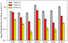 |
Fig. 3 Observed CO-integrated fluxes rescaled to the same distance of 150 pc. The ±3σ rms noise is depicted by the vertical lines with caps. The Y-axis has a log scale. |
5 Discussion
5.1 Best-fit disk parameters derived with DiskFit
5.1.1 Stellar properties and disk geometries
We used the DiskFit model and obtained the best-fit parameters for the seven disks (excluding the complex DG Tau system). The best-fit geometric parameters are presented in Table 4. To fit weak C18O (2–1) emission, the stellar masses, geometric parameters, and temperature profiles were fixed to the best-fit 13CO values (they are indicated by the square brackets in Table 4). As can be clearly seen, for each disk the systemic velocities derived from the CO isotopologues agree with each other, as well as with the literature values. The accuracy of the systemic velocities derived from the 12CO and 13CO lines varies between 4 and 20 m s−1 (Table 2). The agreement with the best-fit values derived by the Gaussian fitting of the Kepler-integrated spectra is in general within ≲ 20 m s−1 for all cases, except for the disks affected by the strong cloud confusion (where Kepler-deprojected spectrum is biased), and the very weak C18O (2–1) emission of IQ Tau.
The best-fit inclination and positional angles agree with the literature values, and are within ≲ 1–4° for the 12CO and 13CO data for all the sources but CY Tau (inclination) and DN Tau (PA), see Table 2. The PA and inclination derived from the 12CO data in DN Tau are larger than those obtained from the 13CO data by ≈2 and 3.6°, respectively. For DL Tau, the 12CO (2–1)-based inclination angle is smaller than the 13CO (2–1)-based value by ≈8°, but it has a large uncertainty of ~18° due to the asymmetry of emission caused by the foreground absorption.
The discrepancy in the best-fit orientation and the inclination of the CO emitting layers affects the best-fit dynamical stellar masses. This leads to the difference of ≲ 5–10% in the inferred masses of CI Tau, CY Tau, DM Tau, IQ Tau and UZ Tau E. The best-fit stellar masses of DL Tau and DN Tau derived from 13CO (2–1), see Table 4.
Furthermore, the best-fit stellar masses agree within ~10% with the literature values (Table 1) for CI Tau, DL Tau (disregarding the 12CO estimate), DM Tau, IQ Tau and UZ Tau E. The best-fit dynamical mass of DN Tau, ≈0.66–0.76 M⊙ agrees with the literature value of 0.87 ± 0.15 M⊙ within the uncertainties. The strongest disagreement between the best-fit mass derived with DiskFit (0.49–0.54 M⊙) and the dynamical value from the literature (0.30 ± 0.02 M⊙ Simon et al. 2017) is found for the CY Tau disk. In contrast to our ≈0.9″ observations with NOEMA, the CY Tau mass in Simon et al. (2017) has been derived by the DiskFit modeling of the ALMA12 CO (2–1) data with a higher ≈0.23″ resolution. Given a low inclination of ≲ 30° and a small disk size of ~200–250 au, it becomes difficult to precisely constrain the inclination from the CO data when the angular resolution is only twice better than the disk radius. In this case, the DiskFit fitting of the NOEMA data resulted in i ~ 24–28°, while for the Simon et al. (2017) ALMA data the DiskFit converged to i ~ 30 ± 2°. The strong absorption toward CY Tau further complicates the fitting of the NOEMA 12CO data.
Finally, the best-fit CO gas radii and the literature values shown in Table 2 agree within ~10–20% for the entire sample. The smallest CO emission sizes are found for the DN Tau (~170–290 au), UZ Tau E (~190–210 au), and IQ Tau (~200– 210 au) systems. The DL Tau and DM Tau disks are the largest, with RCO ~ 500–800 au, which could be explained by their high initial sizes followed by efficient viscous spreading during their evolution (e.g., Shakura & Sunyaev 1973; Lynden-Bell & Pringle 1974; Manara et al. 2023). For CI Tau, CY Tau, IQ Tau and UZ Tau E, the difference between various best-fit RCO is ≲ 40 au. In contrast, for DL Tau, DM Tau, and DN Tau, the disk sizes derived from 12CO (2–1) differ significantly from the sizes inferred from the less bright CO isotopologue lines (by ≳ 100 au). Besides the cloud absorption affecting the observed 12CO emission and the noise affecting minor CO isotopologue data, another reason could be the structure of the disk, namely, the steepness of the surface density profile and the degree of tapering toward the outer edge. For strongly tapered disks, the RCO sizes should be less affected by the S/N of the respective CO data, as well as the photodissociation of CO and opacity effects. Interestingly, in the study of Guilloteau et al. (2011), it has been found from the continuum data modeling that the disks around DM Tau and DL Tau should be less tapered than the disks around CI Tau, CY Tau, and UZ Tau E, supporting our NOEMA observations.
Best-fit parameters of the stellar properties and disk geometry.
5.1.2 CO temperatures, column densities, isotopic ratios, and disk gas masses
The best-fit CO excitation temperature and column density profiles are presented in Table 5 and compared in Fig. 5. The (sub)millimeter CO lines in disks are usually thermalized, and their excitation temperatures are thus close to the gas kinetic temperatures. As can be clearly seen, the derived CO temperatures in the outer disks at r ~ 100 au are low, ~ 17–37 K. Some of the derived temperatures at r = 100 au are below the freeze-out temperature of CO of 20 K. From a theoretical perspective, temperatures below 20 K are expected in the outer, ≳ 100–200 au midplane regions in the disks around cool T Tauri stars (e.g., Kenyon & Hartmann 1987; Birnstiel et al. 2010; Woitke et al. 2016). Moreover, the presence of cold, ≲ 20 K CO gas in the outer disks due to the grain evolution, nonthermal photo- or chemical desorption, or transport processes has been predicted by various detailed disk thermochemical models (e.g., Semenov et al. 2006; Piétu, et al. 2007; Krijt et al. 2020; Woitke et al. 2022; Gavino et al. 2023). Alternatively, these low temperatures could be caused by the single power-law description of the disk temperatures in the DiskFit model, whereas in other disk models aiming at fitting the CO isotopologue or dust continuum emission, a temperature floor values have often been assumed to keep the disk midpane or CO layer temperatures above a certain thermal threshold value (see, e.g., Andrews et al. 2009; Rosenfeld et al. 2013; Williams & Best 2014; Zhang et al. 2017; Schwarz et al. 2018; Tazzari et al. 2021; Miotello et al. 2023; Law et al. 2022).
The best-fit temperature exponents q are usually ~0.4–0.7. The 13CO and C18O lines in CI Tau are an exception, and are more consistent with flat temperature profiles. These values are typical for outer disk regions around cool T Tauri stars (e.g. Henning & Semenov 2013; Dutrey et al. 2014; Miotello et al. 2023). The less optically thin minor CO isotopologues probe a deeper, cooler part of the CO molecular layer, and thus show lower gas temperatures (depending on the vertical structure), see, e.g. Dutrey et al. (2017); Flores et al. (2021). The warmest CO gas is in the CI, DN, DM Tau and UZ Tau E disks, with T ~ 32–37 K. The CI Tau and DN Tau have the highest stellar luminosities in our sample, L* ≈ 0.8 and 0.69 L⊙, respectively, and, hence, should have the warmest disk atmospheres (Table 1). The disk of DM Tau is flared and hence could be more efficiently heated by the central M dwarf star, leading to a stronger temperature gradient (Piétu, et al. 2007). The UZ Tau E disk may have a low gas mass of ≲ 0.003 M⊙ (see Appendix A), but this should not necessarily lead to a warmer CO molecular layer in this disk. A more plausible explanation is that the luminosity of this binary system is higher than ~0.35 L⊙ shown in Table 1. Indeed, a higher luminosity value of ~0.8–2.2 L⊙ have been adopted in other works (Ricci et al. 2010; Guilloteau et al. 2016; Tripathi et al. 2017; Manara et al. 2023).
Rather similar CO temperatures have been found for our disks in other studies. Law et al. (2022) have constrained vertical structures of the CI Tau and DM Tau disks, using archival ≈0.1–0.4″ ALMA data. They have found that the DM Tau disk has an elevated CO emission surface, and inferred the 12CO temperatures between ~20 K in the outer disk and up to ~35 K in the inner disk at r ≲ 100 au. These DM Tau temperatures are also similar to those obtained in the earlier studies of Piétu et al. (2007) and Flaherty et al. (2020). In Law et al. (2023), a detailed analysis of the vertical emission distribution and the gas temperatures using better ≈0.1–0.2″ ALMA observations of the three main CO isotopologues have been performed for several disks, including DM Tau. It has been found that the C18O emission comes from the cold midplane, while the 12CO and 13CO emission comes from elevated heights, z/r ~ 0.2–0.4 (and the 12CO emitting surface is located higher than the 13CO surface). They derived the best-fit12CO and 13CO temperatures at r = 100 au of 38 ± 0.5 and 26 ± 0.4 K, respectively, which our DiskFit values of 31.6 ± 0.1 and 21.4 ± 0.2 K match rather well (see Table 5). The best-fit power-law exponents for the gas temperature profiles of q ≈ 0.42–0.56 have been obtained by Law et al. (2023), which again are well matched by our DiskFit q ≈ 0.51–0.58 values (within uncertainties).
In contrast to DM Tau, the 12CO temperature at r = 100 au in CI Tau derived by Law et al. (2022) is ~48 K, which is warmer than the best-fit 12CO temperature of ~34 K derived in this study (see Table 5). One of the reasons for that is a lower spatial resolution of our 0.9″ NOEMA CO data compared to the −0.1″ ALMA data used by Law et al. (2022), which makes it impossible for the DiskFit model to probe gas properties in the innermost ~50–80 au regions resolved with ALMA. Another reason is that the CO temperature profile constrained from the high-resolution ALMA data deviates from a simple power law in CI Tau, with prominent gas temperature dips at the radii of 70 and 120 au, and a local gas temperature peak at 90 au (this peak coincides with a strong change in the CO surface emission profile and is close to a dust continuum emission ring), see Law et al. (2022). Our coarser NOEMA CO observations do not show these substructures, see Fig. C.1. Hence, the DiskFit model that is not sensitive to these localized temperature deviations and is more strongly dominated by the CO data from the colder, >100 au region tends to underestimate the gas temperature in the inner disk.
The column density profiles at r = 100 au are compared in Fig. 6 and are ~2 × 10¹⁶−1018 cm−2 for 12CO, ~1015− 2 × 1016 cm−2 for 13CO, and ~1014−2 × 1015 cm−2 for C18O, respectively. The power-law exponents of the column density profiles p are ~0.5–3.2 for 12CO and vary between 0.2 and 1.8 for 13CO and C18O. The 12CO (2–1) emission is optically thick, and thus the best-fit 12CO column densities could be underestimated. (Constraints on the 12CO column density come in part from the optically thin line wings, and in part from the power law assumption). The highest 12CO surface densities of ~1018 cm−2 were found in the CI Tau and DM Tau disks, whereas the lowest values of ≲ 1017 cm−2 were found in the disks around CY, DL, DN, IQ Tau, and UZ Tau E. The column densities derived from the less optically thick 13CO (2–1) are the highest for CI Tau, CY Tau, and DM Tau (−2 × 1016 cm−2), and the lowest in DL Tau and IQ Tau (≲ 1015 cm−2). For C18O (2–1), the highest column densities were obtained for CI Tau, DM Tau, and UZ Tau E (~1015 cm−2), while the lowest values were found in DL Tau and IQ Tau (~1014 cm−2). Thus, both the DL Tau and IQ Tau disks have the lowest CO surface densities in our sample. While for the IQ Tau disk it can be explained by its low disk mass of 0.009 M⊙, the situation for DL Tau is more interesting. The combined [CI] and CO observations of DL Tau with ALMA and ACA by Sturm et al. (2022) have revealed that carbon could be severely depleted by a factor of ~50–150 in the outer DL Tau molecular layer. This is consistent with the apparently old age of the DL Tau disk, ~4– 8 Myr, as well as a measured high CO/dust size ratio, indicative of efficient radial drift and dust evolution, and associated chemical processing of CO (Krijt et al. 2020; Powell et al. 2022; Sturm et al. 2022). Another estimate of the CO depletion for our sample has been derived for DM Tau by McClure et al. (2016), who found that the depletion is mild, within a factor of 5 or less.
We used the best-fit column densities and calculated the corresponding isotopic ratios and the 1σ uncertainties for 12CO/13CO and 13CO/C18O (see Fig. 7). Both the 12CO/13CO and 13CO/C18O ratios roughly fall within the ranges observed in disks and the ISM of ~20–165 and ~8–12, respectively (e.g. Piétu, et al. 2007; Booth et al. 2019; Furuya et al. 2022b; Yoshida et al. 2022). The only exception is the 13CO/C18O ratio in DM Tau, where the C18O column density could be underestimated due to the noisy C18O (2–1) data or, perhaps, could be the result of strong selective photodissociation of C18O in the very extended, outer flared disk region (see Fig. C.24).
Finally, we used the best-fit power-law profiles of the 13CO column densities to estimate disk gas masses. Since the best-fit 12CO column densities could be underestimated by DiskFit due to the optical thickness of the 12CO line, we assumed a range of [20–69] for the 12CO/13CO ratios and used it to recalculate the 12CO column densities. CO is heavily frozen-out in the mid-plane of the cold, > 100 au disk regions probed by our NOEMA observations, hence we have adopted a non-ISM 12CO/H2 ratio of ~10−6 to constrain the underlying gas surface density profile (e.g., Semenov & Wiebe 2011; Miotello et al. 2018; Krijt et al. 2020; Trapman et al. 2022). By taking all these assumptions into account, the resulting disk gas masses vary between ~10−3− 0.2 M⊙ with considerable uncertainties, see Table 6. Compared to the rescaled dust masses adopted from the previous studies (see Table 2), the gas masses calculated from our 13CO data are somewhat higher by a factor of ~2–3, except for the disks around DL Tau, DN Tau and IQ Tau, which have lower CO-derived masses compared to their rescaled dust-derived masses. This is not surprising because the DL Tau, DN Tau, and IQ Tau disks have low C18O (2–1) fluxes and low best-fit C18O column densities, indicating a low amount of CO gas. The CO-derived mass of the extended, RCO ~ 620 au disk around DL Tau deviates the most from its dust mass, once again suggesting that this peculiar system may have more severe CO depletion than in other disks (see also Sturm et al. 2022), while the compact disks around DN Tau and IQ Tau have low total gas masses. The most massive disk in our sample is DM Tau with a CO-derived mass of ~0.06–0.2 M⊙, which is somewhat higher than its mass of ≲ 0.045 M⊙ derived from the Herschel HD observations (McClure et al. 2016; Trapman et al. 2017). A more detailed study of the gas densities and masses in PRODIGE sources derived by the physical-chemical modeling will be presented in Franceschi et al. (2024).
Best-fit gas thermal and CO column density profiles.
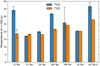 |
Fig. 5 Best-fit gas temperatures and their 1σ uncertainties for the observed 12CO and 13CO isotopologues at a disk radius of 100 au are shown. |
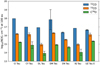 |
Fig. 6 Best-fit column densities and their 1σ uncertainties for the observed CO isotopologues at a disk radius of 100 au are shown. The 12CO column densities can be underestimated due to the optical thickness of the 12CO emission. |
5.2 Correlations between disk physical and chemical properties
In this subsection, we discuss trends among the various disk physical and chemical parameters. Given a modest size of our disk sample with < 10 systems and a biased selection procedure, the results of such analysis should be taken with care. We compared the dust continuum fluxes, CO emission radii, CO temperatures, disk masses derived from dust masses rescaled by an assumed gas/dust ratio of 100, and stellar masses versus the absolute and normalized integrated and peak fluxes, CO column densities, ages, etc., and found only a few potential correlations. For each correlation, we calculated the corresponding coefficient of determination, which is equal to the Pearson coefficient r squared, by taking the data uncertainties when necessary.
First, we compare the 1.3 mm continuum and the rescaled disk dust masses in Fig. 8. As can be clearly seen, despite the fact that dust masses are derived from continuum emission, there is no strong correlation between these quantities due to significant uncertainties in the derived dust masses and a limited disk sample size. A similar absence of a clear correlation was found between the CO-derived gas masses and the dust continuum, again due to gas mass uncertainties. Next, we compare the best-fit CO emission radii with the corresponding integrated and peak fluxes in Fig. 9. While the optically thick 12CO (2–1) data show a potential correlation between the peak flux Sv and the disk gas radius RCO (bottom right panel), for the optically thin CO isotopologues there is a dependence between both the peak and integrated fluxes, and the disk gas radius. In all these cases, the DL Tau disk with its very low CO fluxes (wrt its large, ~600 au CO radius) appears as an outlier. The same trend is visible for the CO fluxes normalized to the dust continuum vs. RCO. The likely interpretation of this potential trend is a combination of similar cold temperatures in the outer regions of our T Tau disk sample, coupled with similar radial CO density profiles off-set by distinct (but yet not too different) absolute CO column densities.
Interestingly, the correlation between the disk radius R and the disk luminosity/flux F, R ∝ F0.5, has been observationally inferred for the dust continuum for many disks in Chamaeleon, Lupus, Ophiuchus, and Taurus, and for the 12CO emission in the Lupus and Upper Scorpius disks (Manara et al. 2023, and references therein). Such a correlation should in general hold when 1) emission is optically thick and 2) the temperature spread is relatively narrow. Manara et al. have mentioned several explanations for such correlation, such as (1) dust grain growth and radial drift in a low viscosity regime or when slowed by pressure bumps in the disk substructures, or (2) the presence of optically thick dust substructures. In the recent study by Zagaria et al. (2023), semi-analytic and detailed DALI thermo-chemical modeling of the disk CO fluxes have been performed, assuming a viscous accretion model and an MHD-wind-based accretion model. They have found that indeed the CO fluxes correlate with the disk radii, which can be constrained from the fluxes even when the disks are not spatially resolved. They have also found that the disk models are able to reproduce the CO fluxes observed in the Lupus star-forming region only when a CO depletion factor of ~40–100 is introduced in the model atop of the ISM abundance xCO = 10−4, which is representative of severe CO depletion and photodissociation in the outer disk regions.
Another quantity that could correlate with the CO isotopo-logue emission radius in our sample is the dust-derived disk mass (see Fig. 10). A naive explanaition for such a trend could be again the radial dust drift and slower depletion of the mm dust reservoirs in larger disks compared to the compact ones. Better statistics regarding disk gas properties from larger, ≳ 30– 50 disks’ observational surveys is needed to verify or falsify our findings.
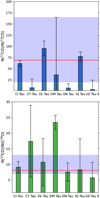 |
Fig. 7 Column density ratios of 12CO/13CO (top) and 13CO/C18O (bottom) at a disk radius of 100 au. The shaded area shows the isotopic ratios measured in disks or the ISM. The local ISM isotopic ratios are shown by the thick red line. |
Disk gas masses derived from the 13CO (2–1) column densities.
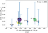 |
Fig. 8 Correlation between the thermal dust continuum fluxes at 1.3 mm and the disk gas masses derived by rescaling disk dust masses. The size of the disk symbol reflects the disk size, and the color of the symbol designates the luminosity of the central star (darker colors correspond to lower luminosities). The coefficient of determination (corresponding to the Pearson coefficient r to the power of two) was calculated by taking the data uncertainties into account and is shown in the top right corner. |
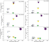 |
Fig. 9 Correlation between the CO gas radii and the integrated (left) and peak (right) fluxes. The 12CO-, 13CO-, and C18O-based data are shown from bottom to top. The size of the disk symbol reflects the disk emission size for the given CO isotopologue, and the color of the symbol designates the luminosity of the central star (darker colors correspond to lower luminosities). The coefficients of determination (corresponding to the Pearson coefficients r to the power of two) were calculated by taking the data uncertainties into account and are shown in the top right corner of each subplot. |
6 Summary and conclusions
We presented the large MPG-IRAM Observatory Program PRODIGE at NOEMA (L19ME; PIs: P. Caselli and Th. Henning), which is aimed at characterizing the properties of eight Class II T Tauri disks in Taurus via a 1 mm line survey (2020–2024). The chosen CI Tau, CY Tau, DG Tau, DL Tau, DM Tau, DN Tau, IQ Tau, and UZ Tau E systems include both compact and extended disks without severe substructures. To deal with a large volume of interferometric data in a coherent manner, we developed the automatic Gildas/Imager pipeline for line selection, imaging, self-calibration, Kepler deprojection, and the S/N boosting. For this first paper, the combined 12CO, 13CO, and C18O J = 2–1 data taken at the 0.9″ and 0.3 km s−1 resolution with the 8–12 mJy beam−1 sensitivity were analyzed and modeled.
We detected the emission of the three main CO isotopo-logues in all the disks (though C18O (2–1) was only marginally detected in IQ Tau). The foreground cloud absorption affects the optically thick 12CO (2–1) emission in CI Tau, CY Tau, DG Tau, DL Tau, and UZ Tau E, and also in 13CO in DL Tau. We spatially resolved the CO emission in all of the disks, and inferred their outer gas radii, ranging from ~200 to 900 au. The peak line brightness temperatures are ~7–16 K for 12CO (2–1), 1–8 K for 13CO (2–1), and 0.2–2 K for C18O (2–1), respectively, indicating that the outer disk gas is cold and that the 13CO (2–1) and C18O (2–1) lines are mostly optically thin.
We found that the CO (2–1) fluxes may scale with the disk outer radius (except that of DL Tau). This may suggest that the assumed radial distribution of the gas is similar in all of our disks, which differ only by the normalization (a total gas mass). The DL Tau system stands out with a large CO radius but faint 13CO and C18O emission. Homogeneous depletion of CO cannot account for this discrepancy and its gas radial distribution should differ from those in the other targeted disks. The UZ Tau E disk shows evidence of non-Keplerian motions, most likely due to the tidal interactions with its UZ Tau W binary companion located ~600 au away.
We fit each line in the Fourier space using the power-law DiskFit model. The discerned gas temperatures at 100 au are low, ~ 17–37 K, and close or slightly above the CO evaporation temperature. The temperatures of the CO molecular layers decline radially with a power-law exponent of ~0.5–0.7. When strong enough, the 13CO (2–1) emission is indicative of a flatter temperature profile with an exponent of ~0–0.4, and it usually has lower temperatures than the temperatures probed by the 12CO line in the extended disks, consistent with the vertical temperature gradients. The difference between the 12CO and 13CO temperatures is not systematic though.
We found that the 12CO, 13CO, and C18O column densities at r = 100 au are ~1017–1018 cm−2, ~1015–1016 cm−2, and ≲1014–1015 cm−2, respectively. The lowest 13CO and C18O column densities were found in the DL Tau and IQ Tau disks. Most disks have a 13CO column density exponent p of about 1.5, with a notable exception for DL Tau, where it is almost zero. The inferred CO column densities point to CO depletion in the outer disk regions. In addition, there could be selective depletion of carbon inside the inner, ≲ 150–200 au, region in the DL Tau disk, making the overall CO budget of this extended ~600 au sized disk much lower than in the other sources. These results support the previous finding based on ALMA observations that CO can be strongly depleted in the DL Tau disk by a factor of ≳100–200 (atop of the depletion due to CO photodissociation and freeze-out).
The best-fit isotopic 12CO/13CO ratios of ~5–80 and the 13CO/C18O ratios of ~6–23 broadly agree within the uncertainties with the previously discerned isotopic values in disks and the local ISM of ~20–165 and ~8–12, respectively. For CI Tau, CY Tau, DM Tau, and UZ Tau E, the disk gas masses estimated from the best-fit 13CO radial profiles and the disk gas radii are ~0.001–0.2 M⊙ (with large uncertainties), and they are a factor of two to three higher than the rescaled dust disk masses.
Finally, we investigated the dependences between various distinct disk and stellar parameters. Owing to the limited size of our sample, the only clear trends that we could identify are between the CO emission sizes and the CO fluxes or disk masses. Similar relations have been found for the 12CO emission observed in the Lupus and Upper Scorpius disks, as well as for the dust continuum observations of disks in the Chamaeleon, Lupus, Ophiuchus, and Taurus star-forming regions.
Acknowledgements
This work is based on observations carried out under project numbers L19ME and S19AW (for DN Tau and CI Tau) with the IRAM NOEMA Interferometer. IRAM is supported by INSU/CNRS (France), MPG (Germany) and IGN (Spain). D.S., Th.H., G.S.-P., R.F, K.S., and S.vT. acknowledge support from the European Research Council under the Horizon 2020 Framework Program via the ERC Advanced Grant No. 832428-Origins. A.F. acknowledges funding from the European Research Council via the ERC advanced grant SUL4LIFE (GAP-101096293). A.F. also thanks the Spanish MICIN for funding from PID2019-106235GB-I00. This work was partly supported by the Programme National “Physique et Chimie du Milieu Interstellaire” (PCMI) of CNRS/INSU with INC/INP co-funded by CEA and CNES. This research made use of NASA’s Astrophysics Data System. Some of the figures in this paper were made with the MATPLOTLIB package (Hunter 2007).
Appendix A Additional information about the disk sample
CI Tau:. The CI Tau system consists of a single star surrounded by a ~175 au dust disk and a ~ 520 au CO gas disk (Long et al. 2018, 2019; Law et al. 2022). The stellar dynamical mass is O.9M⊙, while other mass estimates derived from the stellar models are 0.8 – 1.29M⊙ (Ricci et al. 2010; Simon et al. 2019; Gangi et al. 2022). A hot Jupiter planet with a 9-day orbital period has been found in this system (Johns-Krull et al. 2016; Flagg et al. 2019), making it a (pre-)transitional system. The high-resolution ALMA observations by Clarke et al. (2018); Konishi et al. (2018); Long et al. (2018); Rosotti et al. (2021) have revealed several emission rings and gaps in the dust continuum. The dust gaps with widths of ~9 – 22 are located at radii of ~12 – 14, 39 – 48 and 100 – 120 au, suggesting that there could be up to four planets interacting with the disk. There is a hint for the presence of a 13CO gap at ~60 au (Rosotti et al. 2021). The disk mass derived from dust emission varies between ~0.015 and 0.05 solar masses (Andrews & Williams 2007; Ricci et al. 2010; Guilloteau et al. 2016; Ribas et al. 2020).
CY Tau:. CY Tau is the lowest mass star in our sample, with a dynamical mass of only 0.3M⊙ (Simon et al. 2019). Its mass estimates derived by various stellar models deviate considerably from the dynamical mass, and are ~0.35 – 0.5M⊙ (Ricci et al. 2010; Simon et al. 2019; Pegues et al. 2021). The single CY Tau star is surrounded by a prominent disk with a dust radius of ~100 au and a gas radius of ~200 – 300 au (Guilloteau et al. 2014; Herczeg & Hillenbrand 2014; Guilloteau et al. 2016; Powell et al. 2019). The disk mass derived from dust emission is ~0.01 – 0.077M⊙ (Ricci et al. 2010; Guilloteau et al. 2011, 2016; Ribas et al. 2020). The disk gas mass derived from the fitting the dust lane locations and the disk surface density is 0.06M⊙ (Powell et al. 2019).
DG Tau:. DG Tau is a young, ~0.3 – 0.5 Myr Class I/II object, partly enshrouded by an extended envelope. It shows both thermal and nonthermal radio emission associated with a bipolar jet, an outflow, and shocks (Guilloteau et al. 2012; Purser et al. 2018; Garufi et al. 2022). The stellar mass of the targeted DG Tau star is about 0.8M⊙ (Banzatti et al. 2019). The DG Tau disk has a CO gas radius of ~200 – 300 au (Guilloteau et al. 2011). The disk mass estimates vary wildly, ~0.03 – 0.4M⊙ (Isella et al. 2009; Guilloteau et al. 2011; Ribas et al. 2020).
DL Tau:. DL Tau is the most massive star in our sample, with a dynamical mass M* ≈ 1 M⊙ (non-dynamical mass estimates vary between 0.8 and 1.1M⊙), see Ricci et al. (2010); Long et al. (2018); Simon et al. (2019); Gangi et al. (2022). The DL Tau system has a dust disk with a radius of ~150 au and a gas disk with a radius of ~ 500 au (Long et al. 2018, 2022). The 0.1″ ALMA observations by Long et al. (2018) and Long et al. (2020) have revealed three dust gaps with widths of ~7 – 26 au, located at ~40, 67, and 89 au (Long et al. 2018). Fainter substructures at ≳150 au have been found in the dust emission (Jennings et al. 2022). The derived disk mass from dust observations is ~0.01 −0.1M⊙ (Andrews & Williams 2007; Ricci et al. 2010; Guilloteau et al. 2011). The age of this system is poorly estimated. While Ricci et al. (2010) have derived an age of ~2.2 Myr, which is in agreement with other estimates, McClure (2019) has estimated that the DL Tau system could be much older, ~7.8 Myr.
DM Tau:. The well-studied DM Tau system is a single star with a dynamical mass of 0.55M⊙ surrounded by a large ~200 au dust and a ~600 – 800 au gas disk (Guilloteau et al. 2011; Simon et al. 2019; Long et al. 2020). The age of DM Tau is ~1 – 5 Myr (Guilloteau et al. 2011). The DM Tau disk shows two prominent gaps in dust emission at ~3 and 21 au, with more shallow gaps at ~70, 83 and ~112 au (Kudo et al. 2018; Hashimoto et al. 2021; Francis et al. 2022). The DM Tau disk is turbulent, with discerned α ~ 10−2 – 8 × 10⁻² (Guilloteau et al. 2012; Flaherty et al. 2020; Francis et al. 2022). The disk gas mass derived from the modeling HD (1–0) emission is ~0.004 – 0.045M⊙, depending on the assumed disk thermal structure (McClure et al. 2016; Trapman et al. 2017).
DN Tau:. DN Tau has a dynamical mass of 0.87M⊙ and is surrounded by a disk with a ~100 au dust and a ~240 au gas radius (Ricci et al. 2010; Long et al. 2018; Simon et al. 2019). The dust emission shows the presence of a ~23 au wide gap at ~60 au (Long et al. 2018). The disk mass derived from dust continuum data is ~0.01 – 0.04M⊙ (Guilloteau et al. 2016; Ribas et al. 2020).
IQ Tau:. IQ Tau has a dynamical mass of 0.74M⊙ and is surrounded by a disk with a ~ 100 au dust and a ~220 au gas radius (Ricci et al. 2010; Long et al. 2018; Simon et al. 2019). The non-dynamical mass estimates span a broad range, 0.4 – 0.7M⊙. The IQ Tau disk shows the presence of a ~7 au dust continuum gap at ~40 au (Long et al. 2018). The disk mass derived from dust continuum data is ~0.007 – 0.02M⊙ (Ricci et al. 2010; Guilloteau et al. 2016; Ribas et al. 2020).
UZ Tau E:. UZ Tau E is a spectroscopic binary EXOr system with a separation of ~0.03 au, which is gravitationally linked with another close binary UZ Tau W system at a 3.6″ separation (Hales et al. 2020; Long et al. 2022). The combined mass of the UZ Tau E is 1.2M⊙. The UZ Tau E is surrounded by a disk with a ~80 au dust and a ~200 – 300 au gas radius (Ricci et al. 2010; Long et al. 2022). It has a small inner cavity with a radius of ≲10 au and a shallow, ~ 7 au gap at the radius of ~70 au (Long et al. 2018; Jennings et al. 2022). The dust disk mass is estimated to be ~1 – 2.2 × 10⁻⁴M⊙, while the gas mass derived from the fitting optically thin CO data is ~3.2 × 10⁻³M⊙ (Ricci et al. 2010; Guilloteau et al. 2016; Long et al. 2018; Hales et al. 2020). The high, ~0.03 – 0.07 dust/gas ratio in the UZ Tau E disk is similar to the values found in other EXors as well as Lupus disks (Hales et al. 2020).
Appendix B Spectral setup 1 (2019–2020)
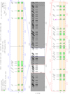 |
Fig. B.1 First NOEMA/PolyFiX setup with an LO frequency of ≈224.9 GHz that has been observed during 2020. The following key disk molecular species have been targeted at the native 62.5 kHz (∼0.1 km s−1) spectral resolution: 12CO, 13CO, C18O, p-H2CO, DCO+, DCN, DNC, c-C3H2, HC3N, N2D+, etc. |
Spectroscopic line parameters for the PolyFiX setup 1 observations (2019–2020).
Summary of the observations.
Appendix C Channel maps, moment 0–th maps, and Kepler plots
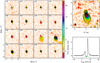 |
Fig. C.1 Observed 12CO (2–1) emission in the CI Tau disk. Shown are the channel map of the observed line brightness distribution (top left), the moment–zero map (top right), and the integrated spectrum (top middle). The channel map shows 16 velocity channels with a step of 0.5 km s−1 in the [−4.5, +4.5] km s−1 range around the systemic velocity. The contour lines start at 2 K, with a step of 2 K. The color bar shows line brightness temperatures (K). The contour lines in the moment–zero plot start at 3, 6, and 9σ with a step of 6σ afterward. The lσ rms noise (mJy km s−1) is shown in the upper left corner of the moment–zero plot, and the synthesized beam is depicted by the dark ellipse in the left bottom corner. The 12CO (2–1) spectrum shows a nearly absent blueshiſted velocity component due to the cloud absorption. |
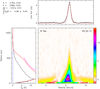 |
Fig. C.2 Observations of 12CO (2–1) emission in the CI Tau disk. Shown is a pixel– deprojected Keplerian plot consisting of the three panels: (left) the radial profile of the line brightness temperature (K), (top) the integrated spectrum (black line) overlaid with the best-fit Gaussian profile (red line), and (bottom right) aligned and stacked line intensity (K) as a function of disk radius (Y-axis; au) and velocity (X-axis; km s−1). The color bar units are in Kelvin. The zigzag behavior of the TB(r) curve at ~200 – 500 au is caused by the foreground cloud absorption. |
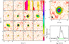 |
Fig. C.7 Observations of 12CO (2−1) emission in the CY Tau disk. Shown are the channel map of the observed line brightness distribution (left), the moment-zero map (top right), and the integrated spectrum (bottom right). The channel map shows 16 velocity channels with a step of 0.5 km s−1 in the [−4.5, +4.5] km s−1 range around the systemic velocity. The contour lines start at 2 K, with a step of 2 K. The color bar shows line brightness temperatures (K). The contour lines in the moment-zero plot start at 3, 6, and 9σ, with a step of 6σ afterward. The 1σ rms noise (mJy km s−1) is shown in the upper left corner of the moment-zero plot, and the synthesized beam is depicted by the dark ellipse in the left bottom corner. |
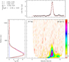 |
Fig. C.8 Observations of 13CO (2−1) emission in the CY Tau disk. Shown are the channel map of the observed line brightness distribution (left), the moment-zero map (top right), and the integrated spectrum (bottom right). The channel map shows 16 velocity channels with a step of 0.5 km s−1 in the [−4.5, +4.5] km s−1 range around the systemic velocity. The contour lines start at 2 K, with a step of 2 K. The color bar shows line brightness temperatures (K). The contour lines in the moment-zero plot start at 3, 6, and 9σ with a step of 6σ afterward. The 1σ rms noise (mJy km s−1) is shown in the upper left corner of the moment-zero plot, and the synthesized beam is depicted by the dark ellipse in the left bottom corner. |
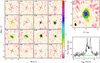 |
Fig. C.9 Observations of 13CO (2−1) emission in the CY Tau disk. Shown are the channel map of the observed line brightness distribution (left), the moment-zero map (top right), and the integrated spectrum (bottom right). The channel map shows 16 velocity channels with a step of 0.5 km s−1 in the [−4.5, +4.5] km s−1 range around the systemic velocity. The contour lines start at 2 K, with a step of 2 K. The color bar shows line brightness temperatures (K). The contour lines in the moment-zero plot start at 3, 6, and 9σ with a step of 6σ afterward. The 1σ rm s noise (mJy km s−1) is shown in the upper left corner of the moment-zero plot, and the synthesized beam is depicted by the dark ellipse in the left bottom corner. |
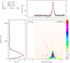 |
Fig. C.10 Observations of 13CO (2−1) emission in the CY Tau disk. Shown is a pixel-deprojected Keplerian plot consisting of the three panels: (left) the radial profile of the line brightness temperature (K), with observations and errorbars in black, and profile derived from the best-fit disk model in red, (top) the integrated spectrum (black line) overlaid with the best-fit Gaussian profile (red line), and (bottom right) aligned and stacked line intensity (K) as a function of disk radius (Y-axis; au) and velocity (X-axis; km s−1). The color bar units are in Kelvin. |
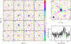 |
Fig. C.11 Observations of C18O (2−1) emission in the CY Tau disk. Shown are the channel map of the observed line brightness distribution (left), the moment-zero map (top right), and the integrated spectrum (bottom right). The channel map shows 16 velocity channels with a step of 0.5 km s−1 in the [−4.5, +4.5] km s−1 range around the systemic velocity. The contour lines start at 2 K, with a step of 2 K. The color bar shows line brightness temperatures (K). The contour lines in the moment-zero plot start at 3, 6, and 9σ, with a step of 6σ afterward. The 1σ rms noise (mJy km s−1) is shown in the upper left corner of the moment-zero plot, and the synthesized beam is depicted by the dark ellipse in the left bottom corner. |
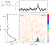 |
Fig. C.12 Observations of C18O (2−1) emission in the CY Tau disk. Shown are the channel map of the observed line brightness distribution (left), the moment-zero map (top right), and the integrated spectrum (bottom right). The channel map shows 16 velocity channels with a step of 0.5 km s−1 in the [−4.5, +4.5] km s−1 range around the systemic velocity. The contour lines start at 2 K, with a step of 2 K. The color bar shows line brightness temperatures (K). The contour lines in the moment-zero plot start at 3, 6, and 9σ with a step of 6σ afterward. The 1σ rms noise (mJy km s−1) is shown in the upper left corner of the moment-zero plot, and the synthesized beam is depicted by the dark ellipse in the left bottom corner. |
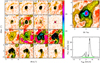 |
Fig. C.13 Observations of 12CO (2−1) emission in the DG Tau disk. Shown are the channel map of the observed line brightness distribution (left), the moment-zero map (top right), and the integrated spectrum (bottom right). The channel map shows 16 velocity channels with a step of 0.5 km s−1 in the [−4.5, +4.5] km s−1 range around the systemic velocity. The contour lines start at 2 K, with a step of 2 K. The color bar shows line brightness temperatures (K). The contour lines in the moment-zero plot start at 3, 6, and 9σ, with a step of 6σ afterward. The 1σ rms noise (mJy km s−1) is shown in the upper left corner of the moment-zero plot, and the synthesized beam is depicted by the dark ellipse in the left bottom corner. |
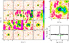 |
Fig. C.14 Observations of 13CO (2−1) emission in the DG Tau disk. Shown are the channel map of the observed line brightness distribution (left), the moment-zero map (top right), and the integrated spectrum (bottom right). The channel map shows 16 velocity channels with a step of 0.5 km s−1 in the [−4.5, +4.5] km s−1 range around the systemic velocity. The contour lines start at 2 K, with a step of 2 K. The color bar shows line brightness temperatures (K). The contour lines in the moment-zero plot start at 3, 6, and 9σ with a step of 6σ afterward. The 1σ rms noise (mJy km s−1) is shown in the upper left corner of the moment-zero plot, and the synthesized beam is depicted by the dark ellipse in the left bottom corner. |
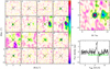 |
Fig. C.15 Observations of C18O (2−1) emission in the DG Tau disk. Shown are the channel map of the observed line brightness distribution (left), the moment-zero map (top right), and the integrated spectrum (bottom right). The channel map shows 16 velocity channels with a step of 0.5 km s−1 in the [−4.5, +4.5] km s−1 range around the systemic velocity. The contour lines start at 2 K, with a step of 2 K. The color bar shows line brightness temperatures (K). The contour lines in the moment-zero plot start at 3, 6, and 9σ, with a step of 6σ afterward. The 1σ rms noise (mJy km s−1) is shown in the upper left corner of the moment-zero plot, and the synthesized beam is depicted by the dark ellipse in the left bottom corner. |
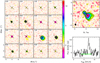 |
Fig. C.16 Observations of 12CO (2−1) emission in the DL Tau disk. Shown are the channel map of the observed line brightness distribution (left), the moment-zero map (top right), and the integrated spectrum (bottom right). The channel map shows 16 velocity channels with a step of 0.5 km s−1 in the [−4.5, +4.5] km s−1 range around the systemic velocity. The contour lines start at 2 K, with a step of 2 K. The color bar shows line brightness temperatures (K). The contour lines in the moment-zero plot start at 3, 6, and 9σ, with a step of 6σ afterward. The 1σ rms noise (mJy km s−1) is shown in the upper left corner of the moment-zero plot, and the synthesized beam is depicted by the dark ellipse in the left bottom corner. |
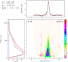 |
Fig. C.17 Observations of 12CO (2–1) emission in the DL Tau disk. Shown is a pixel-deprojected Keplerian plot consisting of the three panels: (left) the radial profile of the line brightness temperature (K), with observations and errorbars in black, and profile derived from the best-fit disk model in red, (top) the integrated spectrum (black line) overlaid with the best-fit Gaussian profile (red line), and (bottom right) aligned and stacked line intensity (K) as a function of disk radius (Y-axis; au) and velocity (X-axis; km s−1). The color bar units are in Kelvin. |
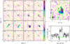 |
Fig. C.18 Observations of 13CO (2–1) emission in the DL Tau disk. Shown are the channel map of the observed line brightness distribution (left), the moment-zero map (top right), and the integrated spectrum (bottom right). The channel map shows 16 velocity channels with a step of 0.5 km s−1 in the [−4.5, +4.5] km s−1 range around the systemic velocity. The contour lines start at 2 K, with a step of 2 K. The color bar shows line brightness temperatures (K). The contour lines in the moment-zero plot start at 3, 6, and 9σ, with a step of 6σ afterward. The 1σ rms noise (mJy km s−1) is shown in the upper left corner of the moment-zero plot, and the synthesized beam is depicted by the dark ellipse in the left bottom corner. |
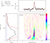 |
Fig. C.19 Observations of 13CO (2–1) emission in the DL Tau disk. Shown is a pixel-deprojected Keplerian plot consisting of the three panels: (left) the radial profile of the line brightness temperature (K), with observations and errorbars in black, and profile derived from the best-fit disk model in red, (top) the integrated spectrum (black line) overlaid with the best-fit Gaussian profile (red line), and (bottom right) aligned and stacked line intensity (K) as a function of disk radius (Y-axis; au) and velocity (X-axis; km s−1). The color bar units are in Kelvin. |
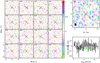 |
Fig. C.20 Observations of C18O (2–1) emission in the DL Tau disk. Shown are the channel map of the observed line brightness distribution (left), the moment-zero map (top right), and the integrated spectrum (bottom right). The channel map shows 16 velocity channels with a step of 0.5 km s−1 in the [−4.5, +4.5] km s−1 range around the systemic velocity. The contour lines start at 2 K, with a step of 2 K. The color bar shows line brightness temperatures (K). The contour lines in the moment-zero plot start at 3, 6, and 9σ, with a step of 6σ afterward. The 1σ rms noise (mJy km s−1) is shown in the upper left corner of the moment-zero plot, and the synthesized beam is depicted by the dark ellipse in the left bottom corner. |
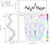 |
Fig. C.21 Observations of C18O (2–1) emission in the DL Tau disk. Shown is a pixel-deprojected Keplerian plot consisting of the three panels: (left) the radial profile of the line brightness temperature (K), with observations and errorbars in black, and profile derived from the best-fit disk model in red, (top) the integrated spectrum (black line) overlaid with the best-fit Gaussian profile (red line), and (bottom right) aligned and stacked line intensity (K) as a function of disk radius (Y-axis; au) and velocity (X-axis; km s−1). The color bar units are in Kelvin. |
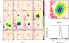 |
Fig. C.22 Observations of 13CO (2–1) emission in the DM Tau disk. Shown are the channel map of the observed line brightness distribution (left), the moment-zero map (top right), and the integrated spectrum (bottom right). The channel map shows 16 velocity channels with a step of 0.5 km s−1 in the [−4.5, +4.5] km s−1 range around the systemic velocity. The contour lines start at 2 K, with a step of 2 K. The color bar shows line brightness temperatures (K). The contour lines in the moment-zero plot start at 3, 6, and 9σ, with a step of 6σ afterward. The 1σ rms noise (mJy km s−1) is shown in the upper left corner of the moment-zero plot, and the synthesized beam is depicted by the dark ellipse in the left bottom corner. |
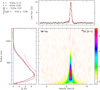 |
Fig. C.23 Observations of 13CO (2–1) emission in the DM Tau disk. Shown is a pixel-deprojected Keplerian plot consisting of the three panels: (left) the radial profile of the line brightness temperature (K), with observations and errorbars in black, and profile derived from the best-fit disk model in red, (top) the integrated spectrum (black line) overlaid with the best-fit Gaussian profile (red line), and (bottom right) aligned and stacked line intensity (K) as a function of disk radius (Y-axis; au) and velocity (X-axis; km s−1). The color bar units are in Kelvin. |
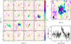 |
Fig. C.24 Observations of C18O (2–1) emission in the DM Tau disk. Shown are the channel map of the observed line brightness distribution (left), the moment-zero map (top right), and the integrated spectrum (bottom right). The channel map shows 16 velocity channels with a step of 0.5 km s−1 in the [−4.5, +4.5] km s−1 range around the systemic velocity. The contour lines start at 2 K, with a step of 2 K. The color bar shows line brightness temperatures (K). The contour lines in the moment-zero plot start at 3, 6, and 9σ, with a step of 6σ afterward. The 1σ rms noise (mJy km s−1) is shown in the upper left corner of the moment-zero plot, and the synthesized beam is depicted by the dark ellipse in the left bottom corner. |
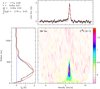 |
Fig. C.25 Observations of C18O (2–1) emission in the DM Tau disk. Shown is a pixel-deprojected Keplerian plot consisting of the three panels: (left) the radial profile of the line brightness temperature (K), with observations and errorbars in black, and profile derived from the best-fit disk model in red, (top) the integrated spectrum (black line) overlaid with the best-fit Gaussian profile (red line), and (bottom right) aligned and stacked line intensity (K) as a function of disk radius (Y-axis; au) and velocity (X-axis; km s−1). The color bar units are in Kelvin. |
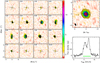 |
Fig. C.26 Observations of 12CO (2–1) emission in the DN Tau disk. Shown are the channel map of the observed line brightness distribution (left), the moment-zero map (top right), and the integrated spectrum (bottom right). The channel map shows 16 velocity channels with a step of 0.5 km s−1 in the [−4.5, +4.5] km s−1 range around the systemic velocity. The contour lines start at 2 K, with a step of 2 K. The color bar shows line brightness temperatures (K). The contour lines in the moment-zero plot start at 3, 6, and 9σ, with a step of 6σ afterward. The 1σ rms noise (mJy km s−1) is shown in the upper left corner of the moment-zero plot, and the synthesized beam is depicted by the dark ellipse in the left bottom corner. |
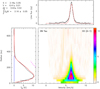 |
Fig. C.27 Observations of 12CO (2–1) emission in the DN Tau disk. Shown is a pixel-deprojected Keplerian plot consisting of the three panels: (left) the radial profile of the line brightness temperature (K), with observations and errorbars in black, and profile derived from the best-fit disk model in red, (top) the integrated spectrum (black line) overlaid with the best-fit Gaussian profile (red line), and (bottom right) aligned and stacked line intensity (K) as a function of disk radius (Y-axis; au) and velocity (X-axis; km s−1). The color bar units are in Kelvin. |
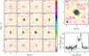 |
Fig. C.28 Observations of 13CO (2–1) emission in the DN Tau disk. Shown are the channel map of the observed line brightness distribution (left), the moment-zero map (top right), and the integrated spectrum (bottom right). The channel map shows 16 velocity channels with a step of 0.5 km s−1 in the [−4.5, +4.5] km s−1 range around the systemic velocity. The contour lines start at 2 K, with a step of 2 K. The color bar shows line brightness temperatures (K). The contour lines in the moment-zero plot start at 3, 6, and 9σ, with a step of 6σ afterward. The 1σ rms noise (mJy km s−1) is shown in the upper left corner of the moment-zero plot, and the synthesized beam is depicted by the dark ellipse in the left bottom corner. |
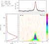 |
Fig. C.29 Observations of 13CO (2–1) emission in the DN Tau disk. Shown is a pixel-deprojected Keplerian plot consisting of the three panels: (left) the radial profile of the line brightness temperature (K), with observations and errorbars in black, and profile derived from the best-fit disk model in red, (top) the integrated spectrum (black line) overlaid with the best-fit Gaussian profile (red line), and (bottom right) aligned and stacked line intensity (K) as a function of disk radius (Y-axis; au) and velocity (X-axis; km s−1). The color bar units are in Kelvin. |
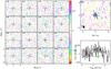 |
Fig. C.30 Observations of C18O (2–1) emission in the DN Tau disk. Shown are the channel map of the observed line brightness distribution (left), the moment-zero map (top right), and the integrated spectrum (bottom right). The channel map shows 16 velocity channels with a step of 0.5 km s−1 in the [−4.5, +4.5] km s−1 range around the systemic velocity. The contour lines start at 2 K, with a step of 2 K. The color bar shows line brightness temperatures (K). The contour lines in the moment-zero plot start at 3, 6, and 9σ, with a step of 6σ afterward. The 1σ rms noise (mJy km s−1) is shown in the upper left corner of the moment-zero plot, and the synthesized beam is depicted by the dark ellipse in the left bottom corner. |
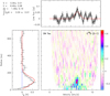 |
Fig. C.31 Observations of C18O (2–1) emission in the DN Tau disk. Shown is a pixel-deprojected Keplerian plot consisting of the three panels: (left) the radial profile of the line brightness temperature (K), with observations and errorbars in black, and profile derived from the best-fit disk model in red, (top) the integrated spectrum (black line) overlaid with the best-fit Gaussian profile (red line), and (bottom right) aligned and stacked line intensity (K) as a function of disk radius (Y-axis; au) and velocity (X-axis; km s−1). The color bar units are in Kelvin. |
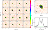 |
Fig. C.32 Observations of 12CO (2–1) emission in the IQ Tau disk. Shown are the channel map of the observed line brightness distribution (left), the moment-zero map (top right), and the integrated spectrum (bottom right). The channel map shows 16 velocity channels with a step of 0.5 km s−1 in the [−4.5, +4.5] km s−1 range around the systemic velocity. The contour lines start at 2 K, with a step of 2 K. The color bar shows line brightness temperatures (K). The contour lines in the moment-zero plot start at 3, 6, and 9σ, with a step of 6σ afterward. The 1σ rms noise (mJy km s−1) is shown in the upper left corner of the moment-zero plot, and the synthesized beam is depicted by the dark ellipse in the left bottom corner. |
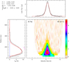 |
Fig. C.33 Observations of 12CO (2−1) emission in the IQ Tau disk. Shown is a pixel-deprojected Keplerian plot consisting of the three panels: (left) the radial profile of the line brightness temperature (K), with observations and errorbars in black, and profile derived from the best-fit disk model in red, (top) the integrated spectrum (black line) overlaid with the best-fit Gaussian profile (red line), and (bottom right) aligned and stacked line intensity (K) as a function of disk radius (Y-axis; au) and velocity (X-axis; km s−1). The color bar units are in Kelvin. |
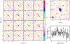 |
Fig. C.34 Observations of 13CO (2–1) emission in the IQ Tau disk. Shown are the channel map of the observed line brightness distribution (left), the moment-zero map (top right), and the integrated spectrum (bottom right). The channel map shows 16 velocity channels with a step of 0.5 km s−1 in the [−4.5, +4.5] km s−1 range around the systemic velocity. The contour lines start at 2 K, with a step of 2 K. The color bar shows line brightness temperatures (K). The contour lines in the moment-zero plot start at 3, 6, and 9σ, with a step of 6σ afterward. The 1σ rms noise (mJy km s−1) is shown in the upper left corner of the moment-zero plot, and the synthesized beam is depicted by the dark ellipse in the left bottom corner. |
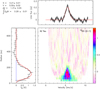 |
Fig. C.35 Observations of 13CO (2–1) emission in the IQ Tau disk. Shown is a pixel-deprojected Keplerian plot consisting of the three panels: (left) the radial profile of the line brightness temperature (K), with observations and errorbars in black, and profile derived from the best-fit disk model in red, (top) the integrated spectrum (black line) overlaid with the best-fit Gaussian profile (red line), and (bottom right) aligned and stacked line intensity (K) as a function of disk radius (Y-axis; au) and velocity (X-axis; km s−1). The color bar units are in Kelvin. |
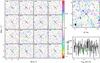 |
Fig. C.36 Observations of C18O (2–1) emission in the IQ Tau disk. Shown are the channel map of the observed line brightness distribution (left), the moment-zero map (top right), and the integrated spectrum (bottom right). The channel map shows 16 velocity channels with a step of 0.5 km s−1 in the [−4.5, +4.5] km s−1 range around the systemic velocity. The contour lines start at 2 K, with a step of 2 K. The color bar shows line brightness temperatures (K). The contour lines in the moment-zero plot start at 3, 6, and 9σ, with a step of 6σ afterward. The 1σ rms noise (mJy km s−1) is shown in the upper left corner of the moment-zero plot, and the synthesized beam is depicted by the dark ellipse in the left bottom corner. |
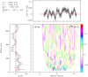 |
Fig. C.37 Observations of C18O (2–1) emission in the IQ Tau disk. Shown is a pixel-deprojected Keplerian plot consisting of the three panels: (left) the radial profile of the line brightness temperature (K), with observations and errorbars in black, and profile derived from the best-fit disk model in red, (top) the integrated spectrum (black line) overlaid with the best-fit Gaussian profile (red line), and (bottom right) aligned and stacked line intensity (K) as a function of disk radius (Y-axis; au) and velocity (X-axis; km s−1). The color bar units are in Kelvin. |
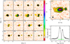 |
Fig. C.38 Observations of 12CO (2–1) emission in the UZ Tau disk. Shown are the channel map of the observed line brightness distribution (left), the moment-zero map (top right), and the integrated spectrum (bottom right). The channel map shows 16 velocity channels with a step of 0.5 km s−1 in the [−4.5, +4.5] km s−1 range around the systemic velocity. The contour lines start at 2 K, with a step of 2 K. The color bar shows line brightness temperatures (K). The contour lines in the moment-zero plot start at 3, 6, and 9σ, with a step of 6σ afterward. The 1σ rms noise (mJy km s−1) is shown in the upper left corner of the moment-zero plot, and the synthesized beam is depicted by the dark ellipse in the left bottom corner. |
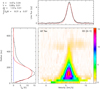 |
Fig. C.39 Observations of 12CO (2–1) emission in the UZ Tau disk. Shown is a pixel-deprojected Keplerian plot consisting of the three panels: (left) the radial profile of the line brightness temperature (K), with observations and errorbars in black, and profile derived from the best-fit disk model in red, (top) the integrated spectrum (black line) overlaid with the best-fit Gaussian profile (red line), and (bottom right) aligned and stacked line intensity (K) as a function of disk radius (Y-axis; au) and velocity (X-axis; km s−1). The color bar units are in Kelvin. |
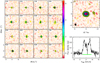 |
Fig. C.40 Observations of 13CO (2–1) emission in the UZ Tau disk. Shown are the channel map of the observed line brightness distribution (left), the moment-zero map (top right), and the integrated spectrum (bottom right). The channel map shows 16 velocity channels with a step of 0.5 km s−1 in the [−4.5, +4.5] km s−1 range around the systemic velocity. The contour lines start at 2 K, with a step of 2 K. The color bar shows line brightness temperatures (K). The contour lines in the moment-zero plot start at 3, 6, and 9σ, with a step of 6σ afterward. The 1σ rms noise (mJy km s−1) is shown in the upper left corner of the moment-zero plot, and the synthesized beam is depicted by the dark ellipse in the left bottom corner. |
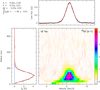 |
Fig. C.41 Observations of 13CO (2–1) emission in the UZ Tau disk. Shown is a pixel-deprojected Keplerian plot consisting of the three panels: (left) the radial profile of the line brightness temperature (K), with observations and errorbars in black, and profile derived from the best-fit disk model in red, (top) the integrated spectrum (black line) overlaid with the best-fit Gaussian profile (red line), and (bottom right) aligned and stacked line intensity (K) as a function of disk radius (Y-axis; au) and velocity (X-axis; km s−1). The color bar units are in Kelvin. |
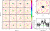 |
Fig. C.42 Observations of C18O (2–1) emission in the UZ Tau disk. Shown are the channel map of the observed line brightness distribution (left), the moment-zero map (top right), and the integrated spectrum (bottom right). The channel map shows 16 velocity channels with a step of 0.5 km s−1 in the [−4.5, +4.5] km s−1 range around the systemic velocity. The contour lines start at 2 K, with a step of 2 K. The color bar shows line brightness temperatures (K). The contour lines in the moment-zero plot start at 3, 6, and 9σ, with a step of 6σ afterward. The 1σ rms noise (mJy km s−1) is shown in the upper left corner of the moment-zero plot, and the synthesized beam is depicted by the dark ellipse in the left bottom corner. |
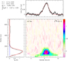 |
Fig. C.43 Observations of C18O (2–1) emission in the UZ Tau disk. Shown is a pixel-deprojected Keplerian plot consisting of the three panels: (left) the radial profile of the line brightness temperature (K), with observations and errorbars in black, and profile derived from the best-fit disk model in red, (top) the integrated spectrum (black line) overlaid with the best-fit Gaussian profile (red line), and (bottom right) aligned and stacked line intensity (K) as a function of disk radius (Y-axis; au) and velocity (X-axis; km s−1). The color bar units are in Kelvin. |
References
- Aikawa, Y., Cataldi, G., Yamato, Y., et al. 2021, ApJS, 257, 13 [NASA ADS] [CrossRef] [Google Scholar]
- ALMA Partnership (Brogan, C. L., et al.) 2015, ApJ, 808, L3 [Google Scholar]
- Anderson, D. E., Cleeves, L. I., Blake, G. A., et al. 2022, ApJ, 927, 229 [NASA ADS] [CrossRef] [Google Scholar]
- Andrews, S. M. 2020, ArA&A, 58, 483 [NASA ADS] [CrossRef] [Google Scholar]
- Andrews, S. M., & Williams, J. P. 2007, ApJ, 659, 705 [NASA ADS] [CrossRef] [Google Scholar]
- Andrews, S. M., Wilner, D. J., Hughes, A. M., Qi, C., & Dullemond, C. P. 2009, ApJ, 700, 1502 [CrossRef] [Google Scholar]
- Andrews, S. M., Huang, J., Pérez, L. M., et al. 2018, ApJ, 869, L41 [NASA ADS] [CrossRef] [Google Scholar]
- Ansdell, M., Williams, J. P., Trapman, L., et al. 2018, ApJ, 859, 21 [NASA ADS] [CrossRef] [Google Scholar]
- Bae, J., Isella, A., Zhu, Z., et al. 2023, in Protostars and Planets VII, eds. S. Inutsuka, Y. Aikawa, T. Muto, K. Tomida, & M. Tamura, Astronomical Society of the Pacific Conference Series, 534, 423 [NASA ADS] [Google Scholar]
- Banzatti, A., Pascucci, I., Edwards, S., et al. 2019, ApJ, 870, 76 [Google Scholar]
- Benisty, M., Dominik, C., Follette, K., et al. 2023, in Protostars and Planets VII, eds. S. Inutsuka, Y. Aikawa, T. Muto, K. Tomida, & M. Tamura, Astronomical Society of the Pacific Conference Series, 534, 605 [NASA ADS] [Google Scholar]
- Bergin, E. A., & Williams, J. P. 2018, arXiv e-prints [arXiv:1807.09631] [Google Scholar]
- Bergin, E., Calvet, N., D’Alessio, P., & Herczeg, G. J. 2003, ApJ, 591, L159 [Google Scholar]
- Bergin, E. A., Cleeves, L. I., Gorti, U., et al. 2013, Nature, 493, 644 [Google Scholar]
- Bergin, E. A., Du, F., Cleeves, L. I., et al. 2016, ApJ, 831, 101 [Google Scholar]
- Bergner, J. B., Öberg, K. I., Guzmán, V. V., et al. 2021, ApJS, 257, 11 [NASA ADS] [CrossRef] [Google Scholar]
- Birnstiel, T., Dullemond, C. P., & Brauer, F. 2010, A&A, 513, A79 [NASA ADS] [CrossRef] [EDP Sciences] [Google Scholar]
- Birnstiel, T., Dullemond, C. P., Zhu, Z., et al. 2018, ApJ, 869, L45 [CrossRef] [Google Scholar]
- Boehler, Y., Ménard, F., Robert, C. M. T., et al. 2021, A&A, 650, A59 [NASA ADS] [CrossRef] [EDP Sciences] [Google Scholar]
- Booth, A. S., Walsh, C., Ilee, J. D., et al. 2019, ApJ, 882, L31 [Google Scholar]
- Bosman, A. D., Alarcón, F., Bergin, E. A., et al. 2021, ApJS, 257, 7 [NASA ADS] [CrossRef] [Google Scholar]
- Calahan, J. K., Bergin, E., Zhang, K., et al. 2021a, ApJ, 908, 8 [NASA ADS] [CrossRef] [Google Scholar]
- Calahan, J. K., Bergin, E. A., Zhang, K., et al. 2021b, ApJS, 257, 17 [NASA ADS] [CrossRef] [Google Scholar]
- Cartledge, S. I. B., Lauroesch, J. T., Meyer, D. M., & Sofia, U. J. 2006, ApJ, 641, 327 [NASA ADS] [CrossRef] [Google Scholar]
- Chapillon, E., Guilloteau, S., Dutrey, A., Piétu, V., & Guélin, M. 2012, A&A, 537, A60 [NASA ADS] [CrossRef] [EDP Sciences] [Google Scholar]
- Clarke, C. J., Tazzari, M., Juhasz, A., et al. 2018, ApJ, 866, L6 [NASA ADS] [CrossRef] [Google Scholar]
- Cleeves, L. I., Bergin, E. A., Qi, C., Adams, F. C., & Öberg, K. I. 2015, ApJ, 799, 204 [CrossRef] [Google Scholar]
- Cleeves, L. I., Öberg, K. I., Wilner, D. J., et al. 2016, ApJ, 832, 110 [Google Scholar]
- Cleeves, L. I., Loomis, R. A., Teague, R., et al. 2021, ApJ, 911, 29 [NASA ADS] [CrossRef] [Google Scholar]
- Dartois, E., Dutrey, A., & Guilloteau, S. 2003, A&A, 399, 773 [CrossRef] [EDP Sciences] [Google Scholar]
- D’Orazi, V., Biazzo, K., & Randich, S. 2011, A&A, 526, A103 [NASA ADS] [CrossRef] [EDP Sciences] [Google Scholar]
- Dutrey, A., Henning, T., Guilloteau, S., et al. 2007, A&A, 464, 615 [NASA ADS] [CrossRef] [EDP Sciences] [Google Scholar]
- Dutrey, A., Semenov, D., Chapillon, E., et al. 2014, Protostars and Planets VI, 317 [Google Scholar]
- Dutrey, A., Guilloteau, S., Piétu, V., et al. 2017, A&A, 607, A130 [CrossRef] [EDP Sciences] [Google Scholar]
- Eistrup, C., & Henning, T. 2022, A&A, 667, A160 [NASA ADS] [CrossRef] [EDP Sciences] [Google Scholar]
- Esplin, T. L., & Luhman, K. L. 2019, AJ, 158, 54 [Google Scholar]
- Facchini, S., Teague, R., Bae, J., et al. 2021, AJ, 162, 99 [NASA ADS] [CrossRef] [Google Scholar]
- Favre, C., Cleeves, L. I., Bergin, E. A., Qi, C., & Blake, G. A. 2013, ApJ, 776, L38 [Google Scholar]
- Fedele, D., & Favre, C. 2020, A&A, 638, A110 [NASA ADS] [CrossRef] [EDP Sciences] [Google Scholar]
- Flagg, L., Johns-Krull, C. M., Nofi, L., et al. 2019, ApJ, 878, L37 [NASA ADS] [CrossRef] [Google Scholar]
- Flaherty, K., Hughes, A. M., Simon, J. B., et al. 2020, ApJ, 895, 109 [NASA ADS] [CrossRef] [Google Scholar]
- Flores, C., Duchêne, G., Wolff, S., et al. 2021, AJ, 161, 239 [NASA ADS] [CrossRef] [Google Scholar]
- Franceschi, R., Birnstiel, T., Henning, T., et al. 2022, A&A, 657, A74 [NASA ADS] [CrossRef] [EDP Sciences] [Google Scholar]
- Franceschi, R., Henning, T., Semenov, D., et al. 2024, A&A, submitted [Google Scholar]
- Francis, L., Marel, N. v. d., Johnstone, D., et al. 2022, AJ, 164, 105 [NASA ADS] [CrossRef] [Google Scholar]
- Furuya, K., Lee, S., & Nomura, H. 2022a, ApJ, 938, 29 [NASA ADS] [CrossRef] [Google Scholar]
- Furuya, K., Tsukagoshi, T., Qi, C., et al. 2022b, ApJ, 926, 148 [NASA ADS] [CrossRef] [Google Scholar]
- Gaia Collaboration (Brown, A. G. A., et al.) 2018, A&A, 616, A1 [NASA ADS] [CrossRef] [EDP Sciences] [Google Scholar]
- Gangi, M., Antoniucci, S., Biazzo, K., et al. 2022, A&A, 667, A124 [NASA ADS] [CrossRef] [EDP Sciences] [Google Scholar]
- Garufi, A., Podio, L., Codella, C., et al. 2022, A&A, 658, A104 [CrossRef] [EDP Sciences] [Google Scholar]
- Gavino, S., Kobus, J., Dutrey, A., et al. 2023, A&A, 680, A59 [NASA ADS] [CrossRef] [EDP Sciences] [Google Scholar]
- Gentaz, O. 2019, in ALMA Development Workshop, 16 [Google Scholar]
- Güdel, M., Eibensteiner, C., Dionatos, O., et al. 2018, A&A, 620, A1 [NASA ADS] [CrossRef] [EDP Sciences] [Google Scholar]
- Guilloteau, S., Dutrey, A., Piétu, V., & Boehler, Y. 2011, A&A, 529, A105 [NASA ADS] [CrossRef] [EDP Sciences] [Google Scholar]
- Guilloteau, S., Dutrey, A., Wakelam, V., et al. 2012, A&A, 548, A70 [CrossRef] [EDP Sciences] [Google Scholar]
- Guilloteau, S., Di Folco, E., Dutrey, A., et al. 2013, A&A, 549, A92 [NASA ADS] [CrossRef] [EDP Sciences] [Google Scholar]
- Guilloteau, S., Simon, M., Piétu, V., et al. 2014, A&A, 567, A117 [NASA ADS] [CrossRef] [EDP Sciences] [Google Scholar]
- Guilloteau, S., Reboussin, L., Dutrey, A., et al. 2016, A&A, 592, A124 [NASA ADS] [CrossRef] [EDP Sciences] [Google Scholar]
- Guzmán, V. V., Öberg, K. I., Loomis, R., & Qi, C. 2015, ApJ, 814, 53 [Google Scholar]
- Haffert, S. Y., Bohn, A. J., de Boer, J., et al. 2019, Nat. Astron., 3, 749 [Google Scholar]
- Hales, A. S., Pérez, S., Gonzalez-Ruilova, C., et al. 2020, ApJ, 900, 7 [NASA ADS] [CrossRef] [Google Scholar]
- Hashimoto, J., Muto, T., Dong, R., et al. 2021, ApJ, 911, 5 [NASA ADS] [CrossRef] [Google Scholar]
- Haworth, T. J., Ilee, J. D., Forgan, D. H., et al. 2016, PASA, 33, e053 [NASA ADS] [CrossRef] [Google Scholar]
- Henning, T., & Semenov, D. 2013, Chem. Rev., 113, 9016 [Google Scholar]
- Henning, T., Semenov, D., Guilloteau, S., et al. 2010, ApJ, 714, 1511 [Google Scholar]
- Herczeg, G. J., & Hillenbrand, L. A. 2014, ApJ, 786, 97 [Google Scholar]
- Hsieh, T. H., Segura-Cox, D. M., Pineda, J. E., et al. 2023, A&A, 669, A137 [NASA ADS] [CrossRef] [EDP Sciences] [Google Scholar]
- Hunter, J. D. 2007, Comput. Sci. Eng., 9, 90 [NASA ADS] [CrossRef] [Google Scholar]
- Isella, A., Carpenter, J. M., & Sargent, A. I. 2009, ApJ, 701, 260 [Google Scholar]
- Jennings, J., Tazzari, M., Clarke, C. J., Booth, R. A., & Rosotti, G. P. 2022, MNRAS, 514, 6053 [NASA ADS] [CrossRef] [Google Scholar]
- Johns-Krull, C. M., McLane, J. N., Prato, L., et al. 2016, ApJ, 826, 206 [Google Scholar]
- Kama, M., Bruderer, S., van Dishoeck, E. F., et al. 2016, A&A, 592, A83 [NASA ADS] [CrossRef] [EDP Sciences] [Google Scholar]
- Kenyon, S. J., & Hartmann, L. 1987, ApJ, 323, 714 [Google Scholar]
- Keppler, M., Benisty, M., Müller, A., et al. 2018, A&A, 617, A44 [NASA ADS] [CrossRef] [EDP Sciences] [Google Scholar]
- Konishi, M., Hashimoto, J., & Hori, Y. 2018, ApJ, 859, L28 [CrossRef] [Google Scholar]
- Krijt, S., Bosman, A. D., Zhang, K., et al. 2020, ApJ, 899, 134 [NASA ADS] [CrossRef] [Google Scholar]
- Kudo, T., Hashimoto, J., Muto, T., et al. 2018, ApJ, 868, L5 [NASA ADS] [CrossRef] [Google Scholar]
- Law, C. J., Loomis, R. A., Teague, R., et al. 2021a, ApJS, 257, 3 [NASA ADS] [CrossRef] [Google Scholar]
- Law, C. J., Teague, R., Loomis, R. A., et al. 2021b, ApJS, 257, 4 [NASA ADS] [CrossRef] [Google Scholar]
- Law, C. J., Crystian, S., Teague, R., et al. 2022, ApJ, 932, 114 [NASA ADS] [CrossRef] [Google Scholar]
- Law, C. J., Teague, R., Öberg, K. I., et al. 2023, ApJ, 948, 60 [NASA ADS] [CrossRef] [Google Scholar]
- Le Gal, R., Öberg, K. I., Loomis, R. A., Pegues, J., & Bergner, J. B. 2019, ApJ, 876, 72 [Google Scholar]
- Le Gal, R., Öberg, K. I., Teague, R., et al. 2021, ApJS, 257, 12 [NASA ADS] [CrossRef] [Google Scholar]
- Lodato, G., Rampinelli, L., Viscardi, E., et al. 2023, MNRAS, 518, 4481 [Google Scholar]
- Long, F., Herczeg, G. J., Pascucci, I., et al. 2017, ApJ, 844, 99 [Google Scholar]
- Long, F., Pinilla, P., Herczeg, G. J., et al. 2018, ApJ, 869, 17 [Google Scholar]
- Long, F., Herczeg, G. J., Harsono, D., et al. 2019, ApJ, 882, 49 [Google Scholar]
- Long, F., Pinilla, P., Herczeg, G. J., et al. 2020, ApJ, 898, 36 [CrossRef] [Google Scholar]
- Long, F., Andrews, S. M., Rosotti, G., et al. 2022, ApJ, 931, 6 [NASA ADS] [CrossRef] [Google Scholar]
- Luhman, K. L. 2018, AJ, 156, 271 [Google Scholar]
- Luhman, K. L. 2023, AJ, 165, 37 [NASA ADS] [CrossRef] [Google Scholar]
- Luhman, K. L., Allen, P. R., Espaillat, C., Hartmann, L., & Calvet, N. 2010, ApJS, 186, 111 [Google Scholar]
- Lynden-Bell, D., & Pringle, J. E. 1974, MNRAS, 168, 603 [Google Scholar]
- Manara, C. F., Ansdell, M., Rosotti, G. P., et al. 2023, in Protostars and Planets VII, ed. S. Inutsuka, Y. Aikawa, T. Muto, K. Tomida, & M. Tamura, Astronomical Society of the Pacific Conference Series, 534, 539 [NASA ADS] [Google Scholar]
- Matrà, L., MacGregor, M. A., Kalas, P., et al. 2017, ApJ, 842, 9 [Google Scholar]
- McClure, M. K. 2019, A&A, 632, A32 [NASA ADS] [CrossRef] [EDP Sciences] [Google Scholar]
- McClure, M. K., Bergin, E. A., Cleeves, L. I., et al. 2016, ApJ, 831, 167 [Google Scholar]
- Miotello, A., Facchini, S., van Dishoeck, E. F., & Bruderer, S. 2018, A&A, 619, A113 [NASA ADS] [CrossRef] [EDP Sciences] [Google Scholar]
- Miotello, A., Facchini, S., van Dishoeck, E. F., et al. 2019, A&A, 631, A69 [NASA ADS] [CrossRef] [EDP Sciences] [Google Scholar]
- Miotello, A., Kamp, I., Birnstiel, T., Cleeves, L. C., & Kataoka, A. 2023, in Protostars and Planets VII, eds. S. Inutsuka, Y. Aikawa, T. Muto, K. Tomida, & M. Tamura, Astronomical Society of the Pacific Conference Series, 534, 501 [NASA ADS] [Google Scholar]
- Mollière, P., Molyarova, T., Bitsch, B., et al. 2022, ApJ, 934, 74 [CrossRef] [Google Scholar]
- Mordasini, C., Alibert, Y., Benz, W., Klahr, H., & Henning, T. 2012, A&A, 541, A97 [NASA ADS] [CrossRef] [EDP Sciences] [Google Scholar]
- Nieva, M. F., & Przybilla, N. 2012, A&A, 539, A143 [NASA ADS] [CrossRef] [EDP Sciences] [Google Scholar]
- Öberg, K. I., & Bergin, E. A. 2016, ApJ, 831, L19 [Google Scholar]
- Öberg, K. I., Qi, C., Wilner, D. J., & Andrews, S. M. 2011, ApJ, 743, 152 [CrossRef] [Google Scholar]
- Öberg, K. I., Guzmán, V. V., Walsh, C., et al. 2021, ApJS, 257, 1 [CrossRef] [Google Scholar]
- Öberg, K. I., Facchini, S., & Anderson, D. E. 2023, ARA&A, 61, 287 [CrossRef] [Google Scholar]
- Paneque-Carreño, T., Miotello, A., van Dishoeck, E. F., et al. 2022, A&A, 666, A168 [NASA ADS] [CrossRef] [EDP Sciences] [Google Scholar]
- Paneque-Carreño, T., Izquierdo, A. F., Teague, R., et al. 2024, A&A, 684, A174 [NASA ADS] [CrossRef] [EDP Sciences] [Google Scholar]
- Pascucci, I., Skinner, B. N., Deng, D., et al. 2023, ApJ, 953, 183 [CrossRef] [Google Scholar]
- Pavlyuchenkov, Y., Semenov, D., Henning, T., et al. 2007, ApJ, 669, 1262 [NASA ADS] [CrossRef] [Google Scholar]
- Pegues, J., Czekala, I., Andrews, S. M., et al. 2021, ApJ, 908, 42 [NASA ADS] [CrossRef] [Google Scholar]
- Phuong, N. T., Dutrey, A., Di Folco, E., et al. 2020, A&A, 635, A9 [EDP Sciences] [Google Scholar]
- Phuong, N. T., Dutrey, A., Chapillon, E., et al. 2021, A&A, 653, A5 [NASA ADS] [CrossRef] [EDP Sciences] [Google Scholar]
- Piétu, V., Dutrey, A., & Guilloteau, S. 2007, A&A, 467, 163 [Google Scholar]
- Pinte, C., Price, D. J., Ménard, F., et al. 2018, ApJ, 860, L13 [Google Scholar]
- Pinte, C., van der Plas, G., Ménard, F., et al. 2019, Nat. Astron., 3, 1109 [NASA ADS] [CrossRef] [Google Scholar]
- Powell, D., Murray-Clay, R., Pérez, L. M., Schlichting, H. E., & Rosenthal, M. 2019, ApJ, 878, 116 [NASA ADS] [CrossRef] [Google Scholar]
- Powell, D., Gao, P., Murray-Clay, R., & Zhang, X. 2022, Nat. Astron., 6, 1147 [CrossRef] [Google Scholar]
- Purser, S. J. D., Ainsworth, R. E., Ray, T. P., et al. 2018, MNRAS, 481, 5532 [NASA ADS] [CrossRef] [Google Scholar]
- Ribas, Á., Espaillat, C. C., Macías, E., & Sarro, L. M. 2020, A&A, 642, A171 [NASA ADS] [CrossRef] [EDP Sciences] [Google Scholar]
- Ricci, L., Testi, L., Natta, A., et al. 2010, A&A, 512, A15 [CrossRef] [EDP Sciences] [Google Scholar]
- Rivière-Marichalar, P., Fuente, A., Le Gal, R., et al. 2020, A&A, 642, A32 [EDP Sciences] [Google Scholar]
- Rosenfeld, K. A., Andrews, S. M., Hughes, A. M., Wilner, D. J., & Qi, C. 2013, ApJ, 774, 16 [Google Scholar]
- Rosotti, G. P., Ilee, J. D., Facchini, S., et al. 2021, MNRAS, 501, 3427 [Google Scholar]
- Rota, A. A., Manara, C. F., Miotello, A., et al. 2022, A&A, 662, A121 [NASA ADS] [CrossRef] [EDP Sciences] [Google Scholar]
- Ruaud, M., Gorti, U., & Hollenbach, D. J. 2022, ApJ, 925, 49 [NASA ADS] [CrossRef] [Google Scholar]
- Schwarz, K. R., Bergin, E. A., Cleeves, L. I., et al. 2018, ApJ, 856, 85 [Google Scholar]
- Schwarz, K. R., Calahan, J. K., Zhang, K., et al. 2021, ApJS, 257, 20 [NASA ADS] [CrossRef] [Google Scholar]
- Semenov, D., & Wiebe, D. 2011, ApJS, 196, 25 [Google Scholar]
- Semenov, D., Wiebe, D., & Henning, T. 2006, ApJ, 647, L57 [NASA ADS] [CrossRef] [Google Scholar]
- Semenov, D., Favre, C., Fedele, D., et al. 2018, A&A, 617, A28 [NASA ADS] [CrossRef] [EDP Sciences] [Google Scholar]
- Shakura, N. I., & Sunyaev, R. A. 1973, A&A, 24, 337 [NASA ADS] [Google Scholar]
- Simon, M., Guilloteau, S., Di Folco, E., et al. 2017, ApJ, 844, 158 [Google Scholar]
- Simon, M., Guilloteau, S., Beck, T. L., et al. 2019, ApJ, 884, 42 [NASA ADS] [CrossRef] [Google Scholar]
- Smirnov-Pinchukov, G. V., Semenov, D. A., Akimkin, V. V., & Henning, T. 2020, A&A, 644, A4 [NASA ADS] [CrossRef] [EDP Sciences] [Google Scholar]
- Stadler, J., Benisty, M., Izquierdo, A., et al. 2023, A&A, 670, L1 [NASA ADS] [CrossRef] [EDP Sciences] [Google Scholar]
- Sturm, J. A., McClure, M. K., Harsono, D., et al. 2022, A&A, 660, A126 [NASA ADS] [CrossRef] [EDP Sciences] [Google Scholar]
- Tazzari, M., Clarke, C. J., Testi, L., et al. 2021, MNRAS, 506, 2804 [NASA ADS] [CrossRef] [Google Scholar]
- Teague, R. 2019, J. Open Source Softw., 4, 1632 [NASA ADS] [CrossRef] [Google Scholar]
- Teague, R., Semenov, D., Guilloteau, S., et al. 2015, A&A, 574, A137 [NASA ADS] [CrossRef] [EDP Sciences] [Google Scholar]
- Teague, R., Guilloteau, S., Semenov, D., et al. 2016, A&A, 592, A49 [CrossRef] [EDP Sciences] [Google Scholar]
- Teague, R., Bae, J., Bergin, E. A., Birnstiel, T., & Foreman-Mackey, D. 2018a, ApJ, 860, L12 [NASA ADS] [CrossRef] [Google Scholar]
- Teague, R., Henning, T., Guilloteau, S., et al. 2018b, ApJ, 864, 133 [NASA ADS] [CrossRef] [Google Scholar]
- Teague, R., Bae, J., Aikawa, Y., et al. 2021, ApJS, 257, 18 [NASA ADS] [CrossRef] [Google Scholar]
- Trapman, L., Miotello, A., Kama, M., van Dishoeck, E. F., & Bruderer, S. 2017, A&A, 605, A69 [NASA ADS] [CrossRef] [EDP Sciences] [Google Scholar]
- Trapman, L., Rosotti, G., Bosman, A. D., Hogerheijde, M. R., & van Dishoeck, E. F. 2020, A&A, 640, A5 [EDP Sciences] [Google Scholar]
- Trapman, L., Zhang, K., van’t Hoff, M. L. R., Hogerheijde, M. R., & Bergin, E. A. 2022, ApJ, 926, L2 [NASA ADS] [CrossRef] [Google Scholar]
- Tripathi, A., Andrews, S. M., Birnstiel, T., & Wilner, D. J. 2017, ApJ, 845, 44 [Google Scholar]
- Turrini, D., Schisano, E., Fonte, S., et al. 2021, ApJ, 909, 40 [Google Scholar]
- Valdivia-Mena, M. T., Pineda, J. E., Segura-Cox, D. M., et al. 2022, A&A, 667, A12 [NASA ADS] [CrossRef] [EDP Sciences] [Google Scholar]
- Van Clepper, E., Bergner, J. B., Bosman, A. D., Bergin, E., & Ciesla, F. J. 2022, ApJ, 927, 206 [NASA ADS] [CrossRef] [Google Scholar]
- Williams, J. P., & Best, W. M. J. 2014, ApJ, 788, 59 [Google Scholar]
- Woitke, P., Min, M., Pinte, C., et al. 2016, A&A, 586, A103 [NASA ADS] [CrossRef] [EDP Sciences] [Google Scholar]
- Woitke, P., Arabhavi, A. M., Kamp, I., & Thi, W. F. 2022, A&A, 668, A164 [NASA ADS] [CrossRef] [EDP Sciences] [Google Scholar]
- Yen, H.-W., Liu, H. B., Gu, P.-G., et al. 2016, ApJ, 820, L25 [CrossRef] [Google Scholar]
- Yoshida, T. C., Nomura, H., Tsukagoshi, T., Furuya, K., & Ueda, T. 2022, ApJ, 937, L14 [CrossRef] [Google Scholar]
- Zagaria, F., Facchini, S., Miotello, A., et al. 2023, A&A, 672, L15 [CrossRef] [EDP Sciences] [Google Scholar]
- Zhang, K., Bergin, E. A., Blake, G. A., Cleeves, L. I., & Schwarz, K. R. 2017, Nat. Astron., 1, 0130 [NASA ADS] [CrossRef] [Google Scholar]
- Zhang, S., Kalscheur, M., Long, F., et al. 2023, ApJ, 952, 108 [NASA ADS] [CrossRef] [Google Scholar]
All Tables
Spectroscopic line parameters for the PolyFiX setup 1 observations (2019–2020).
All Figures
|
Fig. 1 Observations of 12CO (2−1) emission in the DM Tau disk. Shown are the channel map of the observed line brightness distribution (left), the moment-zero map (top right), and the integrated spectrum (bottom right). The channel map shows 16 velocity channels with a step of 0.5 km s−1 in the [−4.5, +4.5] km s−1 range around the systemic velocity. The contour lines start at 2 K, with a step of 2 K. The color bar shows line brightness temperatures (K). The contour lines in the moment-zero plot start at 3, 6, and 9σ, with a step of 6σ afterward. The 1σ rms noise (mJy km s−1) is shown in the upper left corner of the moment-zero plot, and the synthesized beam is depicted by the dark ellipse in the left bottom corner. |
| In the text | |
|
Fig. 2 Observations of 12CO (2−1) emission in the DM Tau disk. Shown is a pixel-deprojected Keplerian plot consisting of the three panels: (left) the radial profile of the line brightness temperature (K) with observations and errorbars in black, and profile derived from the best-fit disk model in red. The magenta dashed curve indicates the expected brightness temperature of an optically thick line derived from temperature power law. Top: the integrated spectrum (black line) overlaid with the best-fit Gaussian profile (red line). Bottom right: aligned and stacked line intensity (K) as a function of disk radius (Y-axis; au) and velocity (X-axis; km s−1). The color bar units are in kelvin. |
| In the text | |
|
Fig. 3 Observed CO-integrated fluxes rescaled to the same distance of 150 pc. The ±3σ rms noise is depicted by the vertical lines with caps. The Y-axis has a log scale. |
| In the text | |
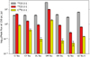 |
Fig. 4 Same as Fig. 3 but for the peak fluxes. |
| In the text | |
|
Fig. 5 Best-fit gas temperatures and their 1σ uncertainties for the observed 12CO and 13CO isotopologues at a disk radius of 100 au are shown. |
| In the text | |
|
Fig. 6 Best-fit column densities and their 1σ uncertainties for the observed CO isotopologues at a disk radius of 100 au are shown. The 12CO column densities can be underestimated due to the optical thickness of the 12CO emission. |
| In the text | |
|
Fig. 7 Column density ratios of 12CO/13CO (top) and 13CO/C18O (bottom) at a disk radius of 100 au. The shaded area shows the isotopic ratios measured in disks or the ISM. The local ISM isotopic ratios are shown by the thick red line. |
| In the text | |
|
Fig. 8 Correlation between the thermal dust continuum fluxes at 1.3 mm and the disk gas masses derived by rescaling disk dust masses. The size of the disk symbol reflects the disk size, and the color of the symbol designates the luminosity of the central star (darker colors correspond to lower luminosities). The coefficient of determination (corresponding to the Pearson coefficient r to the power of two) was calculated by taking the data uncertainties into account and is shown in the top right corner. |
| In the text | |
|
Fig. 9 Correlation between the CO gas radii and the integrated (left) and peak (right) fluxes. The 12CO-, 13CO-, and C18O-based data are shown from bottom to top. The size of the disk symbol reflects the disk emission size for the given CO isotopologue, and the color of the symbol designates the luminosity of the central star (darker colors correspond to lower luminosities). The coefficients of determination (corresponding to the Pearson coefficients r to the power of two) were calculated by taking the data uncertainties into account and are shown in the top right corner of each subplot. |
| In the text | |
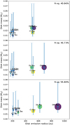 |
Fig. 10 Same as Fig. 9 but for the correlation between the CO gas radii and the disk masses. |
| In the text | |
|
Fig. B.1 First NOEMA/PolyFiX setup with an LO frequency of ≈224.9 GHz that has been observed during 2020. The following key disk molecular species have been targeted at the native 62.5 kHz (∼0.1 km s−1) spectral resolution: 12CO, 13CO, C18O, p-H2CO, DCO+, DCN, DNC, c-C3H2, HC3N, N2D+, etc. |
| In the text | |
|
Fig. C.1 Observed 12CO (2–1) emission in the CI Tau disk. Shown are the channel map of the observed line brightness distribution (top left), the moment–zero map (top right), and the integrated spectrum (top middle). The channel map shows 16 velocity channels with a step of 0.5 km s−1 in the [−4.5, +4.5] km s−1 range around the systemic velocity. The contour lines start at 2 K, with a step of 2 K. The color bar shows line brightness temperatures (K). The contour lines in the moment–zero plot start at 3, 6, and 9σ with a step of 6σ afterward. The lσ rms noise (mJy km s−1) is shown in the upper left corner of the moment–zero plot, and the synthesized beam is depicted by the dark ellipse in the left bottom corner. The 12CO (2–1) spectrum shows a nearly absent blueshiſted velocity component due to the cloud absorption. |
| In the text | |
|
Fig. C.2 Observations of 12CO (2–1) emission in the CI Tau disk. Shown is a pixel– deprojected Keplerian plot consisting of the three panels: (left) the radial profile of the line brightness temperature (K), (top) the integrated spectrum (black line) overlaid with the best-fit Gaussian profile (red line), and (bottom right) aligned and stacked line intensity (K) as a function of disk radius (Y-axis; au) and velocity (X-axis; km s−1). The color bar units are in Kelvin. The zigzag behavior of the TB(r) curve at ~200 – 500 au is caused by the foreground cloud absorption. |
| In the text | |
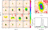 |
Fig. C.3 Same as Fig. C.1 but for 13CO (2−1) emission. |
| In the text | |
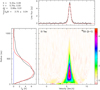 |
Fig. C.4 Same as Fig. C.2 but for 13CO (2−1) emission. |
| In the text | |
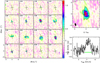 |
Fig. C.5 Same as Fig. C.1 but for C18O (2−1) emission. |
| In the text | |
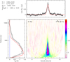 |
Fig. C.6 Same as Fig. C.2 but for C18O (2−1) emission. |
| In the text | |
|
Fig. C.7 Observations of 12CO (2−1) emission in the CY Tau disk. Shown are the channel map of the observed line brightness distribution (left), the moment-zero map (top right), and the integrated spectrum (bottom right). The channel map shows 16 velocity channels with a step of 0.5 km s−1 in the [−4.5, +4.5] km s−1 range around the systemic velocity. The contour lines start at 2 K, with a step of 2 K. The color bar shows line brightness temperatures (K). The contour lines in the moment-zero plot start at 3, 6, and 9σ, with a step of 6σ afterward. The 1σ rms noise (mJy km s−1) is shown in the upper left corner of the moment-zero plot, and the synthesized beam is depicted by the dark ellipse in the left bottom corner. |
| In the text | |
|
Fig. C.8 Observations of 13CO (2−1) emission in the CY Tau disk. Shown are the channel map of the observed line brightness distribution (left), the moment-zero map (top right), and the integrated spectrum (bottom right). The channel map shows 16 velocity channels with a step of 0.5 km s−1 in the [−4.5, +4.5] km s−1 range around the systemic velocity. The contour lines start at 2 K, with a step of 2 K. The color bar shows line brightness temperatures (K). The contour lines in the moment-zero plot start at 3, 6, and 9σ with a step of 6σ afterward. The 1σ rms noise (mJy km s−1) is shown in the upper left corner of the moment-zero plot, and the synthesized beam is depicted by the dark ellipse in the left bottom corner. |
| In the text | |
|
Fig. C.9 Observations of 13CO (2−1) emission in the CY Tau disk. Shown are the channel map of the observed line brightness distribution (left), the moment-zero map (top right), and the integrated spectrum (bottom right). The channel map shows 16 velocity channels with a step of 0.5 km s−1 in the [−4.5, +4.5] km s−1 range around the systemic velocity. The contour lines start at 2 K, with a step of 2 K. The color bar shows line brightness temperatures (K). The contour lines in the moment-zero plot start at 3, 6, and 9σ with a step of 6σ afterward. The 1σ rm s noise (mJy km s−1) is shown in the upper left corner of the moment-zero plot, and the synthesized beam is depicted by the dark ellipse in the left bottom corner. |
| In the text | |
|
Fig. C.10 Observations of 13CO (2−1) emission in the CY Tau disk. Shown is a pixel-deprojected Keplerian plot consisting of the three panels: (left) the radial profile of the line brightness temperature (K), with observations and errorbars in black, and profile derived from the best-fit disk model in red, (top) the integrated spectrum (black line) overlaid with the best-fit Gaussian profile (red line), and (bottom right) aligned and stacked line intensity (K) as a function of disk radius (Y-axis; au) and velocity (X-axis; km s−1). The color bar units are in Kelvin. |
| In the text | |
|
Fig. C.11 Observations of C18O (2−1) emission in the CY Tau disk. Shown are the channel map of the observed line brightness distribution (left), the moment-zero map (top right), and the integrated spectrum (bottom right). The channel map shows 16 velocity channels with a step of 0.5 km s−1 in the [−4.5, +4.5] km s−1 range around the systemic velocity. The contour lines start at 2 K, with a step of 2 K. The color bar shows line brightness temperatures (K). The contour lines in the moment-zero plot start at 3, 6, and 9σ, with a step of 6σ afterward. The 1σ rms noise (mJy km s−1) is shown in the upper left corner of the moment-zero plot, and the synthesized beam is depicted by the dark ellipse in the left bottom corner. |
| In the text | |
|
Fig. C.12 Observations of C18O (2−1) emission in the CY Tau disk. Shown are the channel map of the observed line brightness distribution (left), the moment-zero map (top right), and the integrated spectrum (bottom right). The channel map shows 16 velocity channels with a step of 0.5 km s−1 in the [−4.5, +4.5] km s−1 range around the systemic velocity. The contour lines start at 2 K, with a step of 2 K. The color bar shows line brightness temperatures (K). The contour lines in the moment-zero plot start at 3, 6, and 9σ with a step of 6σ afterward. The 1σ rms noise (mJy km s−1) is shown in the upper left corner of the moment-zero plot, and the synthesized beam is depicted by the dark ellipse in the left bottom corner. |
| In the text | |
|
Fig. C.13 Observations of 12CO (2−1) emission in the DG Tau disk. Shown are the channel map of the observed line brightness distribution (left), the moment-zero map (top right), and the integrated spectrum (bottom right). The channel map shows 16 velocity channels with a step of 0.5 km s−1 in the [−4.5, +4.5] km s−1 range around the systemic velocity. The contour lines start at 2 K, with a step of 2 K. The color bar shows line brightness temperatures (K). The contour lines in the moment-zero plot start at 3, 6, and 9σ, with a step of 6σ afterward. The 1σ rms noise (mJy km s−1) is shown in the upper left corner of the moment-zero plot, and the synthesized beam is depicted by the dark ellipse in the left bottom corner. |
| In the text | |
|
Fig. C.14 Observations of 13CO (2−1) emission in the DG Tau disk. Shown are the channel map of the observed line brightness distribution (left), the moment-zero map (top right), and the integrated spectrum (bottom right). The channel map shows 16 velocity channels with a step of 0.5 km s−1 in the [−4.5, +4.5] km s−1 range around the systemic velocity. The contour lines start at 2 K, with a step of 2 K. The color bar shows line brightness temperatures (K). The contour lines in the moment-zero plot start at 3, 6, and 9σ with a step of 6σ afterward. The 1σ rms noise (mJy km s−1) is shown in the upper left corner of the moment-zero plot, and the synthesized beam is depicted by the dark ellipse in the left bottom corner. |
| In the text | |
|
Fig. C.15 Observations of C18O (2−1) emission in the DG Tau disk. Shown are the channel map of the observed line brightness distribution (left), the moment-zero map (top right), and the integrated spectrum (bottom right). The channel map shows 16 velocity channels with a step of 0.5 km s−1 in the [−4.5, +4.5] km s−1 range around the systemic velocity. The contour lines start at 2 K, with a step of 2 K. The color bar shows line brightness temperatures (K). The contour lines in the moment-zero plot start at 3, 6, and 9σ, with a step of 6σ afterward. The 1σ rms noise (mJy km s−1) is shown in the upper left corner of the moment-zero plot, and the synthesized beam is depicted by the dark ellipse in the left bottom corner. |
| In the text | |
|
Fig. C.16 Observations of 12CO (2−1) emission in the DL Tau disk. Shown are the channel map of the observed line brightness distribution (left), the moment-zero map (top right), and the integrated spectrum (bottom right). The channel map shows 16 velocity channels with a step of 0.5 km s−1 in the [−4.5, +4.5] km s−1 range around the systemic velocity. The contour lines start at 2 K, with a step of 2 K. The color bar shows line brightness temperatures (K). The contour lines in the moment-zero plot start at 3, 6, and 9σ, with a step of 6σ afterward. The 1σ rms noise (mJy km s−1) is shown in the upper left corner of the moment-zero plot, and the synthesized beam is depicted by the dark ellipse in the left bottom corner. |
| In the text | |
|
Fig. C.17 Observations of 12CO (2–1) emission in the DL Tau disk. Shown is a pixel-deprojected Keplerian plot consisting of the three panels: (left) the radial profile of the line brightness temperature (K), with observations and errorbars in black, and profile derived from the best-fit disk model in red, (top) the integrated spectrum (black line) overlaid with the best-fit Gaussian profile (red line), and (bottom right) aligned and stacked line intensity (K) as a function of disk radius (Y-axis; au) and velocity (X-axis; km s−1). The color bar units are in Kelvin. |
| In the text | |
|
Fig. C.18 Observations of 13CO (2–1) emission in the DL Tau disk. Shown are the channel map of the observed line brightness distribution (left), the moment-zero map (top right), and the integrated spectrum (bottom right). The channel map shows 16 velocity channels with a step of 0.5 km s−1 in the [−4.5, +4.5] km s−1 range around the systemic velocity. The contour lines start at 2 K, with a step of 2 K. The color bar shows line brightness temperatures (K). The contour lines in the moment-zero plot start at 3, 6, and 9σ, with a step of 6σ afterward. The 1σ rms noise (mJy km s−1) is shown in the upper left corner of the moment-zero plot, and the synthesized beam is depicted by the dark ellipse in the left bottom corner. |
| In the text | |
|
Fig. C.19 Observations of 13CO (2–1) emission in the DL Tau disk. Shown is a pixel-deprojected Keplerian plot consisting of the three panels: (left) the radial profile of the line brightness temperature (K), with observations and errorbars in black, and profile derived from the best-fit disk model in red, (top) the integrated spectrum (black line) overlaid with the best-fit Gaussian profile (red line), and (bottom right) aligned and stacked line intensity (K) as a function of disk radius (Y-axis; au) and velocity (X-axis; km s−1). The color bar units are in Kelvin. |
| In the text | |
|
Fig. C.20 Observations of C18O (2–1) emission in the DL Tau disk. Shown are the channel map of the observed line brightness distribution (left), the moment-zero map (top right), and the integrated spectrum (bottom right). The channel map shows 16 velocity channels with a step of 0.5 km s−1 in the [−4.5, +4.5] km s−1 range around the systemic velocity. The contour lines start at 2 K, with a step of 2 K. The color bar shows line brightness temperatures (K). The contour lines in the moment-zero plot start at 3, 6, and 9σ, with a step of 6σ afterward. The 1σ rms noise (mJy km s−1) is shown in the upper left corner of the moment-zero plot, and the synthesized beam is depicted by the dark ellipse in the left bottom corner. |
| In the text | |
|
Fig. C.21 Observations of C18O (2–1) emission in the DL Tau disk. Shown is a pixel-deprojected Keplerian plot consisting of the three panels: (left) the radial profile of the line brightness temperature (K), with observations and errorbars in black, and profile derived from the best-fit disk model in red, (top) the integrated spectrum (black line) overlaid with the best-fit Gaussian profile (red line), and (bottom right) aligned and stacked line intensity (K) as a function of disk radius (Y-axis; au) and velocity (X-axis; km s−1). The color bar units are in Kelvin. |
| In the text | |
|
Fig. C.22 Observations of 13CO (2–1) emission in the DM Tau disk. Shown are the channel map of the observed line brightness distribution (left), the moment-zero map (top right), and the integrated spectrum (bottom right). The channel map shows 16 velocity channels with a step of 0.5 km s−1 in the [−4.5, +4.5] km s−1 range around the systemic velocity. The contour lines start at 2 K, with a step of 2 K. The color bar shows line brightness temperatures (K). The contour lines in the moment-zero plot start at 3, 6, and 9σ, with a step of 6σ afterward. The 1σ rms noise (mJy km s−1) is shown in the upper left corner of the moment-zero plot, and the synthesized beam is depicted by the dark ellipse in the left bottom corner. |
| In the text | |
|
Fig. C.23 Observations of 13CO (2–1) emission in the DM Tau disk. Shown is a pixel-deprojected Keplerian plot consisting of the three panels: (left) the radial profile of the line brightness temperature (K), with observations and errorbars in black, and profile derived from the best-fit disk model in red, (top) the integrated spectrum (black line) overlaid with the best-fit Gaussian profile (red line), and (bottom right) aligned and stacked line intensity (K) as a function of disk radius (Y-axis; au) and velocity (X-axis; km s−1). The color bar units are in Kelvin. |
| In the text | |
|
Fig. C.24 Observations of C18O (2–1) emission in the DM Tau disk. Shown are the channel map of the observed line brightness distribution (left), the moment-zero map (top right), and the integrated spectrum (bottom right). The channel map shows 16 velocity channels with a step of 0.5 km s−1 in the [−4.5, +4.5] km s−1 range around the systemic velocity. The contour lines start at 2 K, with a step of 2 K. The color bar shows line brightness temperatures (K). The contour lines in the moment-zero plot start at 3, 6, and 9σ, with a step of 6σ afterward. The 1σ rms noise (mJy km s−1) is shown in the upper left corner of the moment-zero plot, and the synthesized beam is depicted by the dark ellipse in the left bottom corner. |
| In the text | |
|
Fig. C.25 Observations of C18O (2–1) emission in the DM Tau disk. Shown is a pixel-deprojected Keplerian plot consisting of the three panels: (left) the radial profile of the line brightness temperature (K), with observations and errorbars in black, and profile derived from the best-fit disk model in red, (top) the integrated spectrum (black line) overlaid with the best-fit Gaussian profile (red line), and (bottom right) aligned and stacked line intensity (K) as a function of disk radius (Y-axis; au) and velocity (X-axis; km s−1). The color bar units are in Kelvin. |
| In the text | |
|
Fig. C.26 Observations of 12CO (2–1) emission in the DN Tau disk. Shown are the channel map of the observed line brightness distribution (left), the moment-zero map (top right), and the integrated spectrum (bottom right). The channel map shows 16 velocity channels with a step of 0.5 km s−1 in the [−4.5, +4.5] km s−1 range around the systemic velocity. The contour lines start at 2 K, with a step of 2 K. The color bar shows line brightness temperatures (K). The contour lines in the moment-zero plot start at 3, 6, and 9σ, with a step of 6σ afterward. The 1σ rms noise (mJy km s−1) is shown in the upper left corner of the moment-zero plot, and the synthesized beam is depicted by the dark ellipse in the left bottom corner. |
| In the text | |
|
Fig. C.27 Observations of 12CO (2–1) emission in the DN Tau disk. Shown is a pixel-deprojected Keplerian plot consisting of the three panels: (left) the radial profile of the line brightness temperature (K), with observations and errorbars in black, and profile derived from the best-fit disk model in red, (top) the integrated spectrum (black line) overlaid with the best-fit Gaussian profile (red line), and (bottom right) aligned and stacked line intensity (K) as a function of disk radius (Y-axis; au) and velocity (X-axis; km s−1). The color bar units are in Kelvin. |
| In the text | |
|
Fig. C.28 Observations of 13CO (2–1) emission in the DN Tau disk. Shown are the channel map of the observed line brightness distribution (left), the moment-zero map (top right), and the integrated spectrum (bottom right). The channel map shows 16 velocity channels with a step of 0.5 km s−1 in the [−4.5, +4.5] km s−1 range around the systemic velocity. The contour lines start at 2 K, with a step of 2 K. The color bar shows line brightness temperatures (K). The contour lines in the moment-zero plot start at 3, 6, and 9σ, with a step of 6σ afterward. The 1σ rms noise (mJy km s−1) is shown in the upper left corner of the moment-zero plot, and the synthesized beam is depicted by the dark ellipse in the left bottom corner. |
| In the text | |
|
Fig. C.29 Observations of 13CO (2–1) emission in the DN Tau disk. Shown is a pixel-deprojected Keplerian plot consisting of the three panels: (left) the radial profile of the line brightness temperature (K), with observations and errorbars in black, and profile derived from the best-fit disk model in red, (top) the integrated spectrum (black line) overlaid with the best-fit Gaussian profile (red line), and (bottom right) aligned and stacked line intensity (K) as a function of disk radius (Y-axis; au) and velocity (X-axis; km s−1). The color bar units are in Kelvin. |
| In the text | |
|
Fig. C.30 Observations of C18O (2–1) emission in the DN Tau disk. Shown are the channel map of the observed line brightness distribution (left), the moment-zero map (top right), and the integrated spectrum (bottom right). The channel map shows 16 velocity channels with a step of 0.5 km s−1 in the [−4.5, +4.5] km s−1 range around the systemic velocity. The contour lines start at 2 K, with a step of 2 K. The color bar shows line brightness temperatures (K). The contour lines in the moment-zero plot start at 3, 6, and 9σ, with a step of 6σ afterward. The 1σ rms noise (mJy km s−1) is shown in the upper left corner of the moment-zero plot, and the synthesized beam is depicted by the dark ellipse in the left bottom corner. |
| In the text | |
|
Fig. C.31 Observations of C18O (2–1) emission in the DN Tau disk. Shown is a pixel-deprojected Keplerian plot consisting of the three panels: (left) the radial profile of the line brightness temperature (K), with observations and errorbars in black, and profile derived from the best-fit disk model in red, (top) the integrated spectrum (black line) overlaid with the best-fit Gaussian profile (red line), and (bottom right) aligned and stacked line intensity (K) as a function of disk radius (Y-axis; au) and velocity (X-axis; km s−1). The color bar units are in Kelvin. |
| In the text | |
|
Fig. C.32 Observations of 12CO (2–1) emission in the IQ Tau disk. Shown are the channel map of the observed line brightness distribution (left), the moment-zero map (top right), and the integrated spectrum (bottom right). The channel map shows 16 velocity channels with a step of 0.5 km s−1 in the [−4.5, +4.5] km s−1 range around the systemic velocity. The contour lines start at 2 K, with a step of 2 K. The color bar shows line brightness temperatures (K). The contour lines in the moment-zero plot start at 3, 6, and 9σ, with a step of 6σ afterward. The 1σ rms noise (mJy km s−1) is shown in the upper left corner of the moment-zero plot, and the synthesized beam is depicted by the dark ellipse in the left bottom corner. |
| In the text | |
|
Fig. C.33 Observations of 12CO (2−1) emission in the IQ Tau disk. Shown is a pixel-deprojected Keplerian plot consisting of the three panels: (left) the radial profile of the line brightness temperature (K), with observations and errorbars in black, and profile derived from the best-fit disk model in red, (top) the integrated spectrum (black line) overlaid with the best-fit Gaussian profile (red line), and (bottom right) aligned and stacked line intensity (K) as a function of disk radius (Y-axis; au) and velocity (X-axis; km s−1). The color bar units are in Kelvin. |
| In the text | |
|
Fig. C.34 Observations of 13CO (2–1) emission in the IQ Tau disk. Shown are the channel map of the observed line brightness distribution (left), the moment-zero map (top right), and the integrated spectrum (bottom right). The channel map shows 16 velocity channels with a step of 0.5 km s−1 in the [−4.5, +4.5] km s−1 range around the systemic velocity. The contour lines start at 2 K, with a step of 2 K. The color bar shows line brightness temperatures (K). The contour lines in the moment-zero plot start at 3, 6, and 9σ, with a step of 6σ afterward. The 1σ rms noise (mJy km s−1) is shown in the upper left corner of the moment-zero plot, and the synthesized beam is depicted by the dark ellipse in the left bottom corner. |
| In the text | |
|
Fig. C.35 Observations of 13CO (2–1) emission in the IQ Tau disk. Shown is a pixel-deprojected Keplerian plot consisting of the three panels: (left) the radial profile of the line brightness temperature (K), with observations and errorbars in black, and profile derived from the best-fit disk model in red, (top) the integrated spectrum (black line) overlaid with the best-fit Gaussian profile (red line), and (bottom right) aligned and stacked line intensity (K) as a function of disk radius (Y-axis; au) and velocity (X-axis; km s−1). The color bar units are in Kelvin. |
| In the text | |
|
Fig. C.36 Observations of C18O (2–1) emission in the IQ Tau disk. Shown are the channel map of the observed line brightness distribution (left), the moment-zero map (top right), and the integrated spectrum (bottom right). The channel map shows 16 velocity channels with a step of 0.5 km s−1 in the [−4.5, +4.5] km s−1 range around the systemic velocity. The contour lines start at 2 K, with a step of 2 K. The color bar shows line brightness temperatures (K). The contour lines in the moment-zero plot start at 3, 6, and 9σ, with a step of 6σ afterward. The 1σ rms noise (mJy km s−1) is shown in the upper left corner of the moment-zero plot, and the synthesized beam is depicted by the dark ellipse in the left bottom corner. |
| In the text | |
|
Fig. C.37 Observations of C18O (2–1) emission in the IQ Tau disk. Shown is a pixel-deprojected Keplerian plot consisting of the three panels: (left) the radial profile of the line brightness temperature (K), with observations and errorbars in black, and profile derived from the best-fit disk model in red, (top) the integrated spectrum (black line) overlaid with the best-fit Gaussian profile (red line), and (bottom right) aligned and stacked line intensity (K) as a function of disk radius (Y-axis; au) and velocity (X-axis; km s−1). The color bar units are in Kelvin. |
| In the text | |
|
Fig. C.38 Observations of 12CO (2–1) emission in the UZ Tau disk. Shown are the channel map of the observed line brightness distribution (left), the moment-zero map (top right), and the integrated spectrum (bottom right). The channel map shows 16 velocity channels with a step of 0.5 km s−1 in the [−4.5, +4.5] km s−1 range around the systemic velocity. The contour lines start at 2 K, with a step of 2 K. The color bar shows line brightness temperatures (K). The contour lines in the moment-zero plot start at 3, 6, and 9σ, with a step of 6σ afterward. The 1σ rms noise (mJy km s−1) is shown in the upper left corner of the moment-zero plot, and the synthesized beam is depicted by the dark ellipse in the left bottom corner. |
| In the text | |
|
Fig. C.39 Observations of 12CO (2–1) emission in the UZ Tau disk. Shown is a pixel-deprojected Keplerian plot consisting of the three panels: (left) the radial profile of the line brightness temperature (K), with observations and errorbars in black, and profile derived from the best-fit disk model in red, (top) the integrated spectrum (black line) overlaid with the best-fit Gaussian profile (red line), and (bottom right) aligned and stacked line intensity (K) as a function of disk radius (Y-axis; au) and velocity (X-axis; km s−1). The color bar units are in Kelvin. |
| In the text | |
|
Fig. C.40 Observations of 13CO (2–1) emission in the UZ Tau disk. Shown are the channel map of the observed line brightness distribution (left), the moment-zero map (top right), and the integrated spectrum (bottom right). The channel map shows 16 velocity channels with a step of 0.5 km s−1 in the [−4.5, +4.5] km s−1 range around the systemic velocity. The contour lines start at 2 K, with a step of 2 K. The color bar shows line brightness temperatures (K). The contour lines in the moment-zero plot start at 3, 6, and 9σ, with a step of 6σ afterward. The 1σ rms noise (mJy km s−1) is shown in the upper left corner of the moment-zero plot, and the synthesized beam is depicted by the dark ellipse in the left bottom corner. |
| In the text | |
|
Fig. C.41 Observations of 13CO (2–1) emission in the UZ Tau disk. Shown is a pixel-deprojected Keplerian plot consisting of the three panels: (left) the radial profile of the line brightness temperature (K), with observations and errorbars in black, and profile derived from the best-fit disk model in red, (top) the integrated spectrum (black line) overlaid with the best-fit Gaussian profile (red line), and (bottom right) aligned and stacked line intensity (K) as a function of disk radius (Y-axis; au) and velocity (X-axis; km s−1). The color bar units are in Kelvin. |
| In the text | |
|
Fig. C.42 Observations of C18O (2–1) emission in the UZ Tau disk. Shown are the channel map of the observed line brightness distribution (left), the moment-zero map (top right), and the integrated spectrum (bottom right). The channel map shows 16 velocity channels with a step of 0.5 km s−1 in the [−4.5, +4.5] km s−1 range around the systemic velocity. The contour lines start at 2 K, with a step of 2 K. The color bar shows line brightness temperatures (K). The contour lines in the moment-zero plot start at 3, 6, and 9σ, with a step of 6σ afterward. The 1σ rms noise (mJy km s−1) is shown in the upper left corner of the moment-zero plot, and the synthesized beam is depicted by the dark ellipse in the left bottom corner. |
| In the text | |
|
Fig. C.43 Observations of C18O (2–1) emission in the UZ Tau disk. Shown is a pixel-deprojected Keplerian plot consisting of the three panels: (left) the radial profile of the line brightness temperature (K), with observations and errorbars in black, and profile derived from the best-fit disk model in red, (top) the integrated spectrum (black line) overlaid with the best-fit Gaussian profile (red line), and (bottom right) aligned and stacked line intensity (K) as a function of disk radius (Y-axis; au) and velocity (X-axis; km s−1). The color bar units are in Kelvin. |
| In the text | |
Current usage metrics show cumulative count of Article Views (full-text article views including HTML views, PDF and ePub downloads, according to the available data) and Abstracts Views on Vision4Press platform.
Data correspond to usage on the plateform after 2015. The current usage metrics is available 48-96 hours after online publication and is updated daily on week days.
Initial download of the metrics may take a while.