| Issue |
A&A
Volume 684, April 2024
|
|
|---|---|---|
| Article Number | A95 | |
| Number of page(s) | 12 | |
| Section | Stellar structure and evolution | |
| DOI | https://doi.org/10.1051/0004-6361/202348277 | |
| Published online | 08 April 2024 | |
IXPE observation confirms a high spin in the accreting black hole 4U 1957+115
1
Dipartimento di Matematica e Fisica, Università degli Studi Roma Tre, Via della Vasca Navale 84, 00146 Roma, Italy
e-mail: This email address is being protected from spambots. You need JavaScript enabled to view it.
2
Astronomical Institute of the Czech Academy of Sciences, Boční II 1401/1, 14100 Praha 4, Czech Republic
3
Astronomical Institute, Faculty of Mathematics and Physics, Charles University, V Holešovičkách 2, Prague 8 180 00, Czech Republic
4
Institute of Theoretical Physics, Faculty of Mathematics and Physics, Charles University, V Holešovickách 2, 180 00 Praha 8, Czech Republic
5
Physics Department, McDonnell Center for the Space Sciences, and Center for Quantum Leaps, Washington University in St. Louis, St. Louis, MO 63130, USA
6
Center for Astrophysics, Harvard & Smithsonian, 60 Garden St, Cambridge, MA 02138, USA
7
Physics Dept., CB 1105, Washington University, One Brookings Drive, St. Louis, MO 63130-4899, USA
8
INAF – Istituto di Astrofisica e Planetologia Spaziali, Via del Fosso del Cavaliere 100, 00133 Roma, Italy
9
School of Mathematics, Statistics, and Physics, Newcastle University, Newcastle upon Tyne NE1 7RU, UK
10
Université de Strasbourg, CNRS, Observatoire Astronomique de Strasbourg, UMR 7550, 67000 Strasbourg, France
11
Department of Physics and Astronomy, 20014 University of Turku, Finland
12
Dipartimento di Fisica e Astronomia, Università degli Studi di Padova, Via Marzolo 8, 35131 Padova, Italy
13
Nordita, KTH Royal Institute of Technology and Stockholm University, Hannes Alfvéns väg 12, 10691 Stockholm, Sweden
14
California Institute of Technology, Pasadena, CA 91125, USA
15
Space Research Institute of the Russian Academy of Sciences, Profsoyuznaya Str. 84/32, Moscow 117997, Russia
16
INAF – Osservatorio di Astrofisica e Scienza dello Spazio di Bologna, Via P. Gobetti 101, 40129 Bologna, Italy
17
Yamagata University, 1-4-12 Kojirakawa-machi, Yamagata-shi 990-8560, Japan
18
NASA Marshall Space Flight Center, Huntsville, AL 35812, USA
19
NASA Goddard Space Flight Center, Greenbelt, MD 20771, USA
20
Agenzia Spaziale Italiana, Via del Politecnico snc, 00133 Roma, Italy
21
INAF – Osservatorio Astronomico di Cagliari, Via della Scienza 5, 09047 Selargius (CA), Italy
22
Univ. Grenoble Alpes, CNRS, IPAG, 38000 Grenoble, France
23
Dipartimento di Fisica, Università degli Studi di Roma “Tor Vergata”, Via della Ricerca Scientifica 1, 00133 Roma, Italy
24
Istituto Nazionale di Fisica Nucleare, Sezione di Roma “Tor Vergata”, Via della Ricerca Scientifica 1, 00133 Roma, Italy
25
Department of Astronomy, University of Maryland, College Park, Maryland 20742, USA
26
Mullard Space Science Laboratory, University College London, Holmbury St Mary, Dorking, Surrey RH5 6NT, UK
27
Instituto de Astrofísica de Andalucía – CSIC, Glorieta de la Astronomía s/n, 18008 Granada, Spain
28
INAF – Osservatorio Astronomico di Roma, Via Frascati 33, 00040 Monte Porzio Catone (RM), Italy
29
Space Science Data Center, Agenzia Spaziale Italiana, Via del Politecnico snc, 00133 Roma, Italy
30
Istituto Nazionale di Fisica Nucleare, Sezione di Pisa, Largo B. Pontecorvo 3, 56127 Pisa, Italy
31
Dipartimento di Fisica, Università di Pisa, Largo B. Pontecorvo 3, 56127 Pisa, Italy
32
Istituto Nazionale di Fisica Nucleare, Sezione di Torino, Via Pietro Giuria 1, 10125 Torino, Italy
33
Dipartimento di Fisica, Università degli Studi di Torino, Via Pietro Giuria 1, 10125 Torino, Italy
34
INAF – Osservatorio Astrofisico di Arcetri, Largo Enrico Fermi 5, 50125 Firenze, Italy
35
Dipartimento di Fisica e Astronomia, Università degli Studi di Firenze, Via Sansone 1, 50019 Sesto Fiorentino (FI), Italy
36
Istituto Nazionale di Fisica Nucleare, Sezione di Firenze, Via Sansone 1, 50019 Sesto Fiorentino (FI), Italy
37
Science and Technology Institute, Universities Space Research Association, Huntsville, AL 35805, USA
38
Department of Physics and Kavli Institute for Particle Astrophysics and Cosmology, Stanford University, Stanford, CA 94305, USA
39
Institut für Astronomie und Astrophysik, Universität Tüingen, Sand 1, 72076 Tübingen, Germany
40
RIKEN Cluster for Pioneering Research, 2-1 Hirosawa, Wako, Saitama 351-0198, Japan
41
Osaka University, 1-1 Yamadaoka, Suita, Osaka 565-0871, Japan
42
University of British Columbia, Vancouver BC V6T 1Z4, Canada
43
International Center for Hadron Astrophysics, Chiba University, Chiba 263-8522, Japan
44
Institute for Astrophysical Research, Boston University, 725 Commonwealth Avenue, Boston, MA 02215, USA
45
Department of Astrophysics, St. Petersburg State University, Universitetsky pr. 28, Petrodvoretz, 198504 St. Petersburg, Russia
46
Department of Physics and Astronomy and Space Science Center, University of New Hampshire, Durham, NH 03824, USA
47
Istituto Nazionale di Fisica Nucleare, Sezione di Napoli, Strada Comunale Cinthia, 80126 Napoli, Italy
48
MIT Kavli Institute for Astrophysics and Space Research, Massachusetts Institute of Technology, 77 Massachusetts Avenue, Cambridge, MA 02139, USA
49
Graduate School of Science, Division of Particle and Astrophysical Science, Nagoya University, Furo-cho, Chikusa-ku, Nagoya, Aichi 464-8602, Japan
50
Hiroshima Astrophysical Science Center, Hiroshima University, 1-3-1 Kagamiyama, Higashi-Hiroshima, Hiroshima 739-8526, Japan
51
Department of Physics and Astronomy, Louisiana State University, Baton Rouge, LA 70803, USA
52
Department of Physics, University of Hong Kong, Pokfulam, Hong Kong
53
Department of Astronomy and Astrophysics, Pennsylvania State University, University Park, PA 16801, USA
54
INAF – Osservatorio Astronomico di Brera, Via E. Bianchi 46, 23807 Merate (LC), Italy
55
Anton Pannekoek Institute for Astronomy & GRAPPA, University of Amsterdam, Science Park 904, 1098 XH Amsterdam, The Netherlands
56
Guangxi Key Laboratory for Relativistic Astrophysics, School of Physical Science and Technology, Guangxi University, Nanning 530004, PR China
Received:
13
October
2023
Accepted:
18
January
2024
Abstract
We present the results of the first X-ray polarimetric observation of the low-mass X-ray binary 4U 1957+115, performed with the Imaging X-ray Polarimetry Explorer in May 2023. The binary system has been in a high-soft spectral state since its discovery and is thought to host a black hole. The ∼571 ks observation reveals a linear polarisation degree of 1.9%±0.6% and a polarisation angle of −41.°8±7.°9 in the 2–8 keV energy range. Spectral modelling is consistent with the dominant contribution coming from the standard accretion disc, while polarimetric data suggest a significant role of returning radiation: photons that are bent by strong gravity effects and forced to return to the disc surface, where they can be reflected before eventually reaching the observer. In this setting, we find that models with a black hole spin lower than 0.96 and an inclination lower than 50° are disfavoured.
Key words: accretion / accretion disks / black hole physics / polarization / X-rays: binaries / X-rays: individuals: 4U 1957+115
© The Authors 2024
 Open Access article, published by EDP Sciences, under the terms of the Creative Commons Attribution License (https://creativecommons.org/licenses/by/4.0), which permits unrestricted use, distribution, and reproduction in any medium, provided the original work is properly cited.
This article is published in open access under the Subscribe to Open model. This email address is being protected from spambots. You need JavaScript enabled to view it. to support open access publication.
1. Introduction
Low-mass X-ray binaries are binary star systems consisting of a compact object, such as a black hole (BH) or a neutron star, and a low-mass companion from which mass is transferred via Roche-lobe overflow. Most of these systems typically display strong variability in their X-ray emission. A notable exception to this behaviour is represented by 4U 1957+115. Discovered in 1973 by the Uhuru satellite during its scan of the Aquila region (Giacconi et al. 1974), the source is exceptional for being one of a few historically persistently active BH candidates. This short list also includes LMC X-1, LMC X-3, Cyg X-1, and Cyg X-3, which are, unlike 4U 1957+115, classified as high-mass X-ray binary systems (Orosz et al. 2009, 2014; Miller-Jones et al. 2021). In line with the first two of those sources, 4U 1957+115 is always in a soft X-ray spectral state (e.g. Yaqoob et al. 1993; Ricci et al. 1995; Nowak & Wilms 1999; Nowak et al. 2008, 2012; Maitra et al. 2014; Sharma et al. 2021; Barillier et al. 2023). Furthermore, the source has never shown any observable radio jet (Russell et al. 2011), which aligns with the source’s persistent soft state behaviour. Remarkably, the absence of any radio hot spot detection has led to the establishment of the most rigorous upper limits on the radio-to-X-ray flux ratio for a BH in a soft state (Maccarone et al. 2020).
Unfortunately, limited information is available regarding the system’s mass, distance, and inclination; this is due to its persistent nature, which hampers optical measurements of binary parameters, best done during quiescence. Optical emission is likely dominated by the accretion disc (Hakala et al. 2014), but optical observations by Thorstensen (1987) revealed a nearly sinusoidal orbital variation with a period of 9.329 ± 0.011 h and ±20% orbital modulation. Several lines of argument have attributed this phenomenon to the irradiation of the companion star’s surface (Margon et al. 1978) by the accretion disc of the compact object (Bayless et al. 2011; Mason et al. 2012; Gomez et al. 2015). This suggests that, from the perspective of the primary, the secondary star occupies a substantial solid angle, which implies a relatively small separation and thus a relatively low total mass for the binary system. This is consistent with the primary being either a neutron star (Bayless et al. 2011) or a low-mass BH (M < 6.2 M⊙; Gomez et al. 2015); both possibilities are allowed by the ≈0.25–0.3 mass ratio derived by Longa-Peña (2015) through Bowen fluorescence line studies. Although no study of the nature of the compact object has been conclusive, the lack of Type I bursts, pulsations, ‘surface emission’ components, or signatures of a boundary layer emission in the X-ray spectra of the source disfavour the neutron star hypothesis (Maccarone et al. 2020).
According to interstellar medium absorption modelling along the line of sight, the source is believed to be located outside the Galactic plane, at a minimum distance of approximately 5 kpc (Nowak et al. 2008; Yao et al. 2008). In a recent study by Barillier et al. (2023), who analysed the parallax and proper motion data from the Gaia Early Data Release 3 catalogue (Gaia Collaboration 2021) assuming that 4U 1957+115 is located in the Galactic halo, they found that the distance probability distribution peaks at 6 kpc. However, the study revealed a substantial cumulative probability (17%) in the range of 15 to 30 kpc. From this, and from NuSTAR data analysis, they derived a mass probability distribution for the source, 50% of which corresponds to M < 7.2 M⊙. Notably, a significant portion of the mass probability distribution (22%) is found to lie within the ‘mass gap’ of 2–5 M⊙, which is known to contain only a limited number of sources (Özel et al. 2010; Farr et al. 2011; Gomez et al. 2015).
The absence of eclipses and any orbital modulations in the X-ray light curve (Wijnands et al. 2002) allowed for the estimate of an upper limit of between 65° and ≈75° for the source inclination, which is consistent with the model of optical variability (Hakala et al. 1999). Furthermore, this inclination range is also in agreement with the absence of a highly ionised wind (Ponti et al. 2012; Parra et al. 2024). On the other hand, X-ray spectral fitting analyses tend to predict large values for the system’s inclination, such as ∼78° (Maitra et al. 2014). Conversely, several optical modulation studies favour systems with lower inclinations (e.g. ∼13°; Gomez et al. 2015).
As a soft-state source, 4U 1957+115’s X-ray spectrum is dominated by the accretion disc emission, with a minor contribution from a Comptonisation component and weak reflection features (Sharma et al. 2021). A correlation has been observed between the brightness of the source and the contribution of the Comptonised component; by analysing NuSTAR observations, Barillier et al. (2023) described the increasing behaviour of the hard tail with rising flux with two different tracks, with one having significantly stronger tails than the other (e.g. see Figs. 8–10 in Barillier et al. 2023). Their proposed explanation for this correlation is a reduction in the disc hardening factor associated with the increase in the amplitude of the power-law tail; this scenario suggests that electron scattering in a hot corona becomes more important as it diminishes in the upper layers of the optically thick accretion disc. Through the analysis of the reflection component and continuum fitting of the disc component, several estimates of the BH spin in 4U 1957+115 have been obtained. These estimates consistently describe the source as rapidly rotating, with spin values as high as a > 0.9 (Nowak et al. 2012), a > 0.98 (Maitra et al. 2014), a ∼ 0.85 (Sharma et al. 2021), and a = 0.95 (Draghis et al. 2023).
An additional way to obtain valuable information about sources of this class is offered by X-ray polarimetry, which is sensitive to the geometry of the emitting region. In the case of soft-state sources, several studies have proposed the potential use of polarimetric data to constrain the inclination of the accretion disc and the BH spin (Connors & Stark 1977; Stark & Connors 1977; Connors et al. 1980; Dovčiak et al. 2004, 2008; Schnittman & Krolik 2009, 2010; Taverna et al. 2020, 2021; Krawczynski & Beheshtipour 2022; Mikusincova et al. 2023; Loktev et al. 2023). The Imaging X-ray Polarimetry Explorer (IXPE; Weisskopf et al. 2022), a space-based observatory launched on 2021 December 9, has enabled, for the first time, a sensitive X-ray polarimetric study of this class of source. IXPE has already observed several BH X-ray binaries, including Cyg X-1 in the hard state (Krawczynski et al. 2022), Cyg X-3 in the hard and intermediate states with strong reflection features (Veledina et al. 2023), LMC X-1 in the soft state (Podgorný et al. 2023), and 4U 1630−47 in both the high-soft (Ratheesh et al. 2024) and the very high-steep power-law state (Rodriguez Cavero et al. 2023).
We present the first X-ray polarimetric measurement of 4U 1957+115, which was observed by IXPE in May 2023. Simultaneous X-ray observations were also carried out with NICER (Gendreau et al. 2012), NuSTAR (Harrison et al. 2013), and SRG/ART-XC (Pavlinsky et al. 2021), which provided a better spectral coverage. The paper is organised as follows. Section 2 describes the observations and the data reduction techniques. Our spectral and polarimetric analysis is presented in Sect. 3, while Sect. 4 describes the modelling of the polarimetric data assuming different BH spin and system inclination values. In Sect. 5 we analyse the impact of corona emission on the observed polarisation properties of the source. Finally, Sect. 6 summarises the main results of our analysis.
2. Observation and data reduction
4U 1957+115 was observed by IXPE from 2023 May 12–24 (ObsID: 02006601) for a net exposure time of ∼571 ks. IXPE detectors (Soffitta et al. 2021) can measure the Stokes parameters I, Q and U, and they have imaging capabilities that allow for the spatial separation of source and background regions. We obtained Level 2 event files from the HEASARC archive1 and subsequently filtered them for source and background regions using the xpselect tool from the IXPEOBSSIM software package (version 30.5, Baldini et al. 2022). For the source extraction regions, circular regions with a radius of 60″ were chosen for each detector unit. The background regions were defined as annuli with an inner radius of 180″ and an outer radius of 280″. We utilised the IXPEOBSSIM PHA1 algorithm to generate weighted Stokes I, Q, and U parameters, which were binned into 11 bins with sizes 0.5 keV in 2–7 keV, except for the last 7–8 keV bin, for which it was 1 keV Polarisation cubes were generated using the unweighted pcube algorithm (Baldini et al. 2022). In this way, the energy-dependent polarisation degree (PD) and polarisation angle (PA) were created. To ensure significant detection in all bins except the last one, we created the PD and PA for five energy bins with a bin size of 1 keV in 2–6 keV for all but the last, 6–8 keV bin, which was 2 keV.
NICER is a large area 0.2–12 keV X-ray timing mission on the International Space Station. Its X-ray Timing Instrument (XTI) is composed of 56 co-aligned focal-plane modules (FPMs), 52 of which have been functional since its launch in 2017. Each FPM houses a silicon drift detector and is paired to a single-bounce concentrator optic. The XTI is collimated to sample a field of view approximately 3 arcmin in radius. Because NICER is a non-imaging instrument, the background is modelled rather than sampled directly (Remillard et al. 2022). We adopted the SCORPEON background model in our analysis2, via the niscorpspect utility.
NICER observed 4U 1957+115 over the duration of the IXPE campaign, in continuous observations typically lasting ∼10 min, up to 40 min. These observations were processed using nicerl2 with standard screening except for the undershoot and overshoot rate filters, which were left unrestricted during this initial stage of the processing. Data during South Atlantic Anomaly passages were reduced separately, but not automatically excluded from analysis. All resulting observations were separated into continuous interval good time intervals (GTIs). For each GTI, the per-FPM distributions of undershoot, overshoot, and X-ray rates were compared across the detector ensemble and any detector presenting a > 10 robust standard deviation outlier for any of the rates was excised from analysis. Between one and seven detectors were screened out for each interval, owing to elevated undershoot rates associated with optical contamination. Detector 63 was particularly affected. Events from the remaining detectors were summed to produce spectra with associated response products. Any GTI of < 100 s duration or exhibiting an elevated background (as screened by eye) was removed. Surviving the screening, in total we obtain approximately 58 ks of good NICER time, 96 GTIs, spread among 12 ObsIDs. Spectra and responses of all GTIs for a given ObsID were summed in weighted combination for analysis.
NuSTAR (Harrison et al. 2013) observed the source with its two co-aligned X-ray telescopes with corresponding Focal Plane Module A (FPMA) and B (FPMB) in three separate observations. The net exposure times for these observations were 18.7 ks (ObsID: 30902042002), 20.2 ks (ObsID: 30902042004) and 19.7 ks (ObsID: 30902042006), respectively. We generated cleaned event files using the dedicated nupipeline task and the most recent calibration files (CALDB 20230516). We performed background subtraction extracting the background from a circular region with a standard radius of 60″ for both detectors and for all observations. The source extraction radius was set at 123″, 123″ and 118″ for the three observations following a procedure that maximises the signal-to-noise ratio (Piconcelli et al. 2004). Subsequently, we re-binned the spectra using the standard task ftgrouppha, implementing the optimal scheme proposed by Kaastra & Bleeker (2016), with the additional requirement of a minimum signal-to-noise ratio of 3 in each bin. The FPMA and FPMB spectra were fitted independently in the spectral analysis, but are combined in plots for clarity.
The Mikhail Pavlinsky ART-XC telescope (Pavlinsky et al. 2021) on board the SRG observatory (Sunyaev et al. 2021) observed the source twice on May 13 and May 21, for 68 and 67 ks, respectively. The data were reduced with the ARTPRODUCTS v1.0 package and CALDB version V20220908. Light curves in 4–8 and 8–16 keV bands were extracted from a 2 arcmin circular region, centred on the source. Data from all seven mirror modules were combined.
Throughout the entire paper, uncertainties are reported at the 90% confidence level, unless explicitly mentioned otherwise. Upper and lower limits are provided at the 99.7% (3σ) confidence level for one parameter of interest.
3. Data analysis
3.1. Timing and spectral analysis
Simultaneously with IXPE observations, we monitored the source in the X-rays with the following instruments and energy bands: NICER (0.3–12 keV), NuSTAR (3–20 keV) and SRG/ART-XC (4–30 keV). IXPE and NICER cover the soft X-ray band and NuSTAR and ART-XC the hard X-ray band over a period of 14 days. The binning size of each instrument is 1 ks for NuSTAR, 623 s for NICER, and 6 ks for IXPE. We see from Fig. 1 that the flux significantly increases in the soft X-ray band on the first three days of monitoring with NICER and IXPE, and then fluctuates around an average value on the last 10 days. In the hard X-ray band, the count rate for NuSTAR appears generally constant within the error bars, while a count rate increase is observed between the two ART-XC observations.
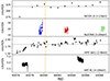 |
Fig. 1. Light curves of 4U 1957+115 as seen by NICER in the 0.3–12 keV energy band, NuSTAR in 3–20 keV, IXPE in 2–8 keV, and ART-XC in 4–12 keV. NuSTAR data coloured in blue, red, and green refer to the three epochs described in the spectral analysis and used in the spectra shown in Fig. 3. The vertical orange line shows the subdivision of the IXPE observation described in Sect. 3.2, and the dashed horizontal lines in the NICER and IXPE light curves indicate the mean values of the count rate. |
In order to analyse the change of state of the source, we calculate the hardness ratio defined as the ratio between the hard energy band over the soft energy band. We define the respective hard/soft energy bands for each instrument: IXPE 5–8 keV/2–5 keV, NICER 4–12 keV/0.3–4 keV, NuSTAR 10–20 keV/3–10 keV, and ART-XC 10–20 keV/4–10 keV. Figure 2 shows the evolution of the hardness ratio calculated from the IXPE, NICER, NuSTAR, and ART-XC data. The IXPE hardness ratio fluctuates between 0.030 and 0.045 over the whole period of observation. For NICER, the hardness ratio varies between 0.052 and 0.054. By calculating the null hypothesis probability fitted with a constant, we have a p-value of 0.0024 for NICER and 4.7003 × 10⁻⁵ for IXPE. Therefore, for NICER the hardness ratio remains constant within the error bars but is more variable for IXPE. Regarding NuSTAR, the hardness ratio decreases from 0.045 to 0.02 in 10 days, indicating a slight transition of the source towards a softer state. The ART-XC hardness ratio slowly increases at the start of the observations and decreases at the end, which is in agreement with the results from NuSTAR.
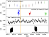 |
Fig. 2. Time evolution of the hardness ratio from NICER, NuSTAR, IXPE, and ART-XC data as defined in the text. NuSTAR and NICER data coloured in blue, red, and green refer to the three epochs described in the spectral analysis and used in the spectra shown in Fig. 3. The vertical orange line shows the subdivision of the IXPE observation described in Sect. 3.2. |
For the spectral analysis of our source, we focused on NuSTAR and NICER simultaneous observations, as indicated in Figs. 1 and 2, performing a joint fit of the spectra of the two satellites. As the NuSTAR high energy flux decreases during the three observations, we adopted different energy ranges according to the energy at which the background starts dominating: 3–30 keV in Period 1, 3–25 keV in Period 2 and 3–20 keV in Period 3. For the NICER data, we fitted the spectra in the 0.7–8 keV energy range for all periods. We used the XSPEC package (v12.13.0c; Arnaud 1996) and employed the following model in the analysis:
 (1)
(1)
In addition, a cross-calibration constant was included to account for discrepancies between the NuSTAR FPMA, FPMB, and NICER spectra. This constant was kept fixed at 1 for the NuSTAR FPMA, while the best-fitting values for NuSTAR FPMB and NICER are 0.981 ± 0.005 and 0.940 ± 0.005, respectively. The spectral model includes a tbabs (Wilms et al. 2000) component to account for interstellar absorption. A kerrbb component is used to describe the accretion disc emission, properly accounting for relativistic effects (Li et al. 2005); this component describes the radiation emitted from the accretion disc assuming that its structure and its emission properties are described accurately by the standard Novikov & Thorne (1973) model. A powerlaw component was included as a phenomenological representation of the Comptonised emission originating from the corona, which was convolved with an expabs component to include a low-energy roll-off. The roll-off energy was obtained in a preliminary analysis using diskbb in place of kerrbb and equating it to the inner disc temperature. This initial modelling with diskbb revealed a large disc emission peak temperature (1.39 ± 0.02, 1.41 ± 0.02, and 1.44 ± 0.02 keV in Periods 1, 2, and 3, respectively), which are typical for this source (Sharma et al. 2021; Barillier et al. 2023).
Disc continuum fitting often encounters substantial degeneracy among various spectral parameters. These parameters encompass the BH mass, distance, accretion rate, hardening factor, system inclination and BH spin. This challenge is notably pronounced in the case of this source, primarily because of the limited availability of robust constraints regarding mass and distance (Barillier et al. 2023). Several analyses disfavour configurations with low spin and/or inclination values due to the broad spectral peak in the disc emission typically observed in this source (Maitra et al. 2014; Sharma et al. 2021). In our analysis, we initially left the system inclination free to vary in the fitting procedure; the best fit was obtained for the maximum value allowed by the model (i = 85°). However, the lack of any X-ray evidence for binary orbital modulation (Wijnands et al. 2002) suggests that the source inclination cannot exceed ≈75°; thus we decided to freeze the inclination of the system to i = 75°, following the approach used in the X-ray analysis performed by Nowak et al. (2008, 2012). We kept the BH spin, its mass and the distance free to vary in the fitting procedure, together with the accretion rate, while we assumed a value of 1.7 for the hardening factor. Due to the strong degeneracy between mass and distance, however, this procedure yielded very large uncertainties on both parameters. Since the main purpose of this work is to analyse the polarimetric data of our source, for the sake of simplicity we decided to fix the mass and distance to the best fiducial values obtained by Barillier et al. (2023) combining Gaia parallax measurements with the NuSTAR spectral analysis: MBH = 4.6 M⊙ and D = 7.8 kpc. Additionally, due to the decline in high-energy flux during the second and third NuSTAR observations (see Fig. 2), the powerlaw photon index Γ became difficult to constrain in these periods. Hence, we linked it across all three observations, while permitting the powerlaw normalisation to vary independently for each period.
However, the fit is statistically unacceptable with χ2/d.o.f. = 2136/953, primarily due to substantial residuals in NICER spectra below 3 keV. These residuals are usually attributed to calibration issues, as similar occurrences have been noted in past observations of this source (Barillier et al. 2023) and other accreting BHs (Podgorný et al. 2023; Rodriguez Cavero et al. 2023). Given that Model (1) effectively describes NuSTAR data (χ2/d.o.f. = 470/438), we decided to address the large residuals by adjusting the response file gains in NICER spectra (using the gain fit command in XSPEC)3. Moreover, we assigned 1% systematic uncertainties for the NICER datasets, within the mission recommendations4, resulting in a revised χ2/d.o.f. = 975.4/951. The optimal spectral parameter values are detailed in Table 1, and the unfolded spectra along with the data-model residuals are shown in Fig. 35.
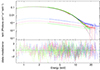 |
Fig. 3. NICER and NuSTAR spectra of 4U 1957+115. Top panel: unfolded spectra (i.e. the flux F(E)) for the best-fitting model described by Model 1 during Periods 1, 2, and 3, shown in red, blue, and green, respectively. The total model for each period, the contributions of the kerrbb and the powerlaw models are shown with the solid, dotted and dashed lines, respectively. Bottom panel: model minus data residuals in units of σ. |
Best-fitting parameters obtained in the spectral analysis of NICER and NuSTAR data during the three periods of observation.
Our spectral analysis allowed us to decompose the spectra into a dominating soft component, representing the accretion disc emission, and a weak hard tail, describing the photons scattered in the corona. While the disc accretion rate exhibits only a slight variation between the three NuSTAR observations, the powerlaw normalisation shows a decrease between the first and the second periods, as suggested by the hardness ratio shown in Fig. 2. This is further reflected by the 2–8 keV flux contribution of the hard component, which goes from 2.3% in Period 1 to 1.0 and 0.7% in Periods 2 and 3, respectively. Significantly, this analysis did not reveal any discernible reflection features. However, it is noteworthy that previous studies of this source have demonstrated that incorporating relativistic reflection models often enhances the overall fit quality (Draghis et al. 2023). Nonetheless, delving into this detailed investigation lies beyond the intended scope of this paper and is deferred to a future publication.
3.2. Polarimetric analysis
The IXPE observation of 4U 1957+115 revealed an average PD in the 2–8 keV band of 1.9%±0.6% at a PA of  , with a statistical significance of 5.2σ. The measurement exceeds the minimum detectable polarisation threshold, MDP99, which is the degree of polarisation that can be determined with a 99% probability against the null hypothesis (Weisskopf et al. 2010). In our observation, the MDP99 within the 2–8 keV band is 1.14%. Figure 4 displays the time-averaged polarisation properties in four energy bands: 2–3, 3–4.3, 4.3–6, 6–8 keV; the first three bins show a slight increase in PD with energy, while the fourth bin shows data below the MDP99 for that energy range, resulting in an upper PD limit. Meanwhile, the PA exhibits a decline within the 2–3 keV and the 3–4.3 keV energy bands, after which it remains relatively constant within statistical uncertainties.
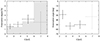 |
Fig. 4. Measured PD (left) and PA (right) of 4U 1957+115, shown with 1σ error bars. The shaded grey area in the PD-plot is an estimate of the MDP99, which shows a significant polarisation measurement from 2 keV up to 6 keV. |
Since the spectral analysis revealed a variation of the hard component during the first part of the IXPE observation, we tried to subdivide the IXPE data to investigate possible time variability of the polarisation. We found that in the initial part of the observation, marked in Figs. 1 and 2 and roughly corresponding to the increase in flux detected in IXPE and NICER light curves, we were unable to significantly detect polarisation, as the polarisation strength was below the MDP99 of 2.06% in that time interval. Subsequently, throughout the remaining observation period, the polarisation properties remained steady, with a PD slightly exceeding that calculated for the entire duration of the IXPE observation (refer to Table 2). Because the polarisation properties identified in these distinct periods aligned, within statistical uncertainties, with the findings from the total observation, for the sake of simplicity we decided to conduct our polarimetric analysis using the entire IXPE observation dataset. This choice is also motivated by the relatively little variation of the accretion disc emission observed in the spectral analysis, leading us to assume that the polarimetric properties of the soft component do not exhibit significant variability during the observation.
3.3. Spectro-polarimetric analysis
We now incorporate the polarimetric information provided by IXPE into our spectral fit. In this section, we take the first exploratory step of fitting a spectro-polarimetric model to the IXPE Q and U spectra. For this purpose, we first incorporated IXPE I spectra into the fitting procedure using Model (1). Given that the IXPE observation extends over a longer time frame compared to the NuSTAR and NICER observations utilised in the spectral fitting detailed in Sect. 3.1, we made the decision to maintain all spectral parameters fixed at the values documented in Table 1. The only exceptions to this were the disc accretion rate and the normalisation of the powerlaw component, which we allowed to vary, together with IXPE data cross-calibration constants. The values obtained for the mass accretion rate and for the powerlaw component normalisation are shown in Table 3; both are consistent with the values obtained in the spectral analysis described in Sect. 3.1. The best-fitting values of the calibration constant are 0.82 ± 0.01, 0.78 ± 0.01, and 0.72 ± 0.01 for IXPE DU1, DU2, and DU3, respectively. As was already noticed in other accreting BHs (Krawczynski et al. 2022; Podgorný et al. 2023; Rodriguez Cavero et al. 2023), a simple constant is not enough to account for cross-calibration uncertainties between IXPE, NICER, and NuSTAR; for this reason, we performed a fit on the response file gains of IXPE spectra6. The fit resulted in a χ2/d.o.f. = 436/442. As a following step, we incorporated the IXPE Q and U spectra in our analysis, adopting our best-fit spectral model and applying the same gains and the same cross calibration factors as for the I spectra. We assigned a constant PD and PA to the model using a polconst component7, and performed a fit in the same four energy bands defined in Sect. 3.2, leaving only the PD and PA of the polconst model as free parameters. Figure 5 shows the contours, calculated using 50 steps for each parameter, in the polar plot of PD and PA. The PD shows a slight increase with energy as in Fig. 4, while the PA is found to have a constant behaviour, within statistical uncertainties. To determine the statistical significance of the observed increase in PD, we conducted a comparison by fitting the Q and U spectra across the entire IXPE energy range. We considered scenarios where PD and PA were either held constant or allowed to vary. When both PD and PA were held constant across energy, the resulting χ2/d.o.f. was 82.7/64. Allowing PD to vary while keeping PA constant improved the fit (χ2/d.o.f. = 74.6/63), while permitting changes in both PD and PA did not significantly enhance the fit, yielding χ2/d.o.f. = 72.7/62. Using an F-test to compare these models, we found that the model that allows PD to vary while maintaining a constant PA is preferred over the model with constant PD and PA, at a confidence level of 99%.
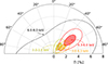 |
Fig. 5. Polar plot of the PD and PA, assuming the spectral best-fit model, in four energy bins: 2.0–3.0, 3.0–4.3, 4.3–6.0, and 6.0–8.0 keV. The shaded and unshaded regions show the 68% and 99.9% confidence areas, respectively, in the first three energy bins. The dashed line indicates the 99.9% confidence level upper limit in the fourth energy bin. |
We then proceeded to incorporate in the fit a physical model that self-consistently describes the spectro-polarimetric properties of the thermal emission. We replaced kerrbb with the model kynbbrr. Similar to kerrbb, kynbbrr assumes a standard Novikov & Thorne (1973) disc model. However, it provides descriptions for both the spectral and polarimetric properties of the emitted radiation. The disc local radiation is assumed to be polarised as in an electron-scattering dominated semi-infinite atmosphere (Chandrasekhar 1960; Sobolev 1963). This model is an extension of the relativistic package KYN (Dovčiak et al. 2004, 2008) developed to include the contribution of returning radiation (Schnittman & Krolik 2009; Taverna et al. 2020). The returning radiation contribution is regulated by the albedo parameter, which describes the fraction of returning photons reflected from the disc surface while the remainder are absorbed. For a more detailed theoretical description of the model, we refer to Mikusincova et al. (2023) and references therein.
To implement this model in the analysis we first used it to fit the IXPE I spectra, leaving only the accretion rate and the normalisation as free parameters. The best-fitting values for these parameters are shown in Table 3. The fit resulted in χ2/d.o.f. = 488/445, assuming no contribution from the returning radiation (albedo=0); the resulting spectral fit was insensitive to variation of the albedo parameter. This absence of a spectral signature attributed to the returning radiation component deviates from recent findings in soft state BH outbursts. In these contexts, returning radiation has been proposed as a plausible source for observed relativistic reflection features, as seen in studies like (Connors et al. 2020, 2021; Lazar et al. 2021). These investigations, alongside theoretical predictions by Dauser et al. (2022), characterised the returning radiation component using the relxillNS model, an evolution of the relxill suite of relativistic reflection models that assumes a single-temperature black-body as the incident radiation source. The discrepancy in results likely arises from the crucial difference in the way reflection is treated in the two models: while kynbbrr describes the reflection process using Chandrasekhar (1960) diffuse reflection formulae, presuming a completely ionised disc atmosphere (see also Taverna et al. 2020), it lacks the capacity to replicate any reflection features in the spectra, as relxillNS does. Since we have not found any apparent reflection features present in the spectra, we consider the use of this pure scattering approximation in our spectro-polarimetric analysis justified. This choice is reinforced by the Taverna et al. (2021) results, which indicate that, due to higher temperatures and lower plasma densities, the matter within the inner regions of rapidly rotating BHs accretion discs is anticipated to be almost entirely ionised.
As the parameters obtained were consistent with the values obtained with Model (1), we extracted from the code the theoretical prediction for the thermal emission PD and PA, presented in Fig. 6. As the self-irradiation contribution becomes more significant, the PD shows an increase with energy due to the large PD expected for this component. Simultaneously, the PA exhibits a 90° rotation with energy, as the returning photons are expected to be polarised perpendicularly to the ones that directly reach the observer after leaving the disc atmosphere. If the albedo parameter is large enough, this rotation occurs below 2 keV, leading to a relatively constant behaviour of the PA with energy in the IXPE energy interval (Taverna et al. 2020). Subsequently, we froze all the spectral parameters of the model and focused on the fit of IXPE Q and U spectra. We employed a polconst model to describe the hard component polarisation properties and left its parameters free to vary in the fit together with the kynbbrr albedo and orientation (χ0) parameter, which indicates the accretion disc axis position angle. We obtained a χ2/d.o.f. = 73.4/62, for the best-fit values detailed in Table 3. However, the soft component albedo and the hard component PD and PA remained unconstrained during the fitting procedure. This can be understood by looking at the contour plots presented in Fig. 7, which shows the 68%, 90%, and 99% confidence level contours for the allowed values of the hard component PD and the albedo parameter. The contours indicate a degeneracy between the two parameters, suggesting two different ways to explain the increasing trend of the PD with energy: either a very large PD of the hard component or a strong contribution from returning radiation.
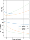 |
Fig. 6. PD (top) and PA (bottom) predicted by the kynbbrr model for the disc emission, assuming all system parameters are fixed at their respective best-fitting values (see Table 1). The different colours indicate different contributions of the returning radiation component, regulated by the albedo parameter. The vertical dashed lines highlight the 2–8 keV energy range. Here, the PA is defined with respect to the disc axis position angle χ0. |
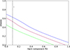 |
Fig. 7. Contour plot of the corona emission PD and the kynbbrr albedo parameter, which regulates the returning radiation contribution. Blue, red, and green lines indicate 68%, 90%, and 99% confidence levels for two parameters of interest, respectively, while the black cross indicates the best-fitting parameters. The dotted vertical line represents the assumed upper limit on the corona emission PD, as described in Sect. 3.3. |
The polarisation properties of coronal emission are influenced by various factors, such as its geometry, optical depth, location, and velocity (see e.g. Zhang et al. 2022). Assuming a flat corona geometry, theoretical studies suggest that the polarisation vector aligns with the disc axis (Poutanen & Svensson 1996; Schnittman & Krolik 2010; Krawczynski & Beheshtipour 2022). This is indeed what has been found in the IXPE observation of Cyg X–1 in the hard state (Krawczynski et al. 2022). This alignment results in the polarisation vector being parallel to that of the returning radiation and perpendicular to the disc direct emission (Schnittman & Krolik 2009; Taverna et al. 2020). Additionally, the IXPE observation of 4U 1630−47 in the steep power-law state measured a PD of the coronal emission of about 7% (Rodriguez Cavero et al. 2023). Considering the similarities between these two sources, both being accreting BH systems likely observed at large inclination angles, we imposed an upper limit of 10% on the PD of the hard component of 4U 1957+115. With this assumption, the only viable explanation for the polarimetric data is the inclusion of returning radiation. Hence, our polarimetric fit shows that the standard thin disc model can effectively describe the polarimetric data of this source, but it is necessary to consider the contribution from self-irradiation (assuming a 10% PD for the corona emission, we find a lower limit of 0.73 for the albedo parameter).
As detailed in Sect. 3.2, the initial part of our IXPE observation did not yield a detectable polarisation signal, as outlined in Table 2. Notably, our first NuSTAR observation, which displays the largest hard component contribution to the spectra, occurred near the end of this period. Considering the reduced hard component contribution during the rest of the observation, the observed low PD might be explained by depolarisation of radiation from the accretion disc by the corona emission. A similar situation was observed in LMC X-1, where the low PD detected by IXPE was attributed to the combination of two spectral components, disc and corona emission, polarised perpendicularly to each other (Podgorný et al. 2023). To investigate this scenario, we attempted to independently fit the polarimetric data in the first period. We made the assumption that the polarisation characteristics of the thermal emission remained constant throughout the observation and represented them using the best-fitting kynbbrr model, derived from our analysis of the entire IXPE observation. Employing a polconst component to characterise the polarisation properties of the hard component, we estimate an upper limit on the PD of 17% during the initial phase of the IXPE observation when assuming the corona emission to be polarised in the direction of the disc axis. This upper limit increased to 38% in the perpendicular configuration.
4. Spin and inclination constraints
Polarimetric data are known to be highly sensitive to the space-time of the emitting region. This is particularly true when considering accreting BHs in soft states because the dominant component of the X-ray spectra originates from photons emitted in the inner regions of the accretion disc, where the strong gravity around the central object significantly alters the observed polarisation properties (Connors & Stark 1977; Stark & Connors 1977; Connors et al. 1980). General relativity effects cause the photon polarisation vectors to undergo rotation as they propagate along geodesics, resulting in a net depolarisation of the emission at infinity and an overall rotation of the PA. Additionally, the already mentioned contribution of returning radiation can profoundly impact the polarimetric signature of the observed radiation (Schnittman & Krolik 2009). These effects are expected to be stronger for the high-energy photons emitted closer to the central BH, introducing an energy dependence on the observed polarisation properties of the thermal emission that provides a mean to estimate the extent of the accretion disc near the BH. In soft-state sources, it is widely believed that the accretion disc extends down to the innermost stable circular orbit (ISCO; Tanaka & Lewin 1995; Steiner et al. 2010), making polarimetric data a valuable tool for estimating the BH spin in such sources via the well-known relation between the ISCO radius and spin (e.g. Fabian & Lasenby 2019). Furthermore, the inclination of the accretion disc also significantly influences the observed polarimetric properties, making modelling of polarimetric data crucial in extracting information about this parameter (Dovčiak et al. 2008; Taverna et al. 2020).
The polarimetric fit described in Sect. 3.3 indicates that the standard Novikov-Thorne thin disc model (Novikov & Thorne 1973; Kato et al. 2008), assuming the large spin and inclination values found in the spectral analysis described in Sect. 3.1, successfully explains the polarimetric data. Here, our goal is to test whether the standard thin disc model can effectively describe the polarimetric data for different values for the BH spin and the disc inclination.
To model the polarimetric data with kynbbrr, we repeated the procedure described in Sect. 3.3, but this time we explored different values for the BH spin and the system inclination. The spectral fit favoured configurations with large spin and inclination values, so when we reduced these parameters’ values, we had to relax some of the initial assumptions on the model to achieve an acceptable fit. Specifically, we allowed the source distance and disc hardening factor to vary freely, as they tend to increase significantly when considering lower spin and inclination values, albeit above the limits suggested by Gaia parallax measurements (Maccarone et al. 2020; Barillier et al. 2023) and disc atmosphere modelling (Shimura & Takahara 1995).
Figure 8 displays the soft component PD and PA predicted by the kynbbrr fit for different spin and inclination values. As the BH spin decreases, the ISCO location moves further away from the central BH. Consequently, the fraction of photons forced to return to the disc surface diminishes. When the BH spin becomes sufficiently low (a ≲ 0.96), the contribution of returning radiation is no longer sufficient to explain the increase in PD with energy, and its primary effect is to depolarise the direct emission. On the other hand, when the disc inclination angle decreases, the observed PD decreases across the entire IXPE band, while the PA exhibits larger rotations with energy. We conducted a polarimetric fit on the IXPE Q and U spectra while assuming different values for the BH spin and the disc inclination. Our analysis identified that the configuration with spin a = 0.998 and disc inclination i = 75° provided the most accurate description of the data, resulting in a χ2/d.o.f. of 72.5/62. On the other hand, the best polarimetric fit assuming spin a = 0.5 resulted in the notably larger χ2/d.o.f. = 79.2/62; furthermore, this configuration demands an exceptionally high PD for the corona component, with a determined lower limit of 51%. When assuming the fiducial value of 10%, the χ2/d.o.f. increases to 84.9/63. This considerably worse fit results from the absence of a significant increase in energy of the PD within the IXPE energy band, as illustrated in the leftmost column of Fig. 8. Figures 9 and 10 present the chi-squared values and contour plots between the PD of the corona emission and the kynbbrr albedo parameter for four different combinations of these parameters. As the BH spin or the disc inclination angle decreases, a larger corona PD is required to account for the PD increase with energy. Notably, for cases where a < 0.96 or when assuming a disc inclination lower than 50°, the corona PD exceeds the upper limit of 10% that we discussed in Sect. 3.3. Consequently, assuming a standard thin disc model, these configurations are disfavoured.
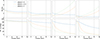 |
Fig. 8. PD (top row) and PA (bottom row) predicted by the kynbbrr model for the disc emission assuming different values for the BH spin and for the system inclination (from left to right): a = 0.5 and i = 75°, a = 0.96 and i = 75°, a = 0.998 and i = 75°, and a = 0.998 and i = 50°. The different colours indicate different contributions of the returning radiation component, regulated by the albedo parameter. The vertical dashed lines highlight the 2–8 keV energy range. Here, the PA is defined with respect to the disc axis position angle χ0. |
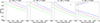 |
Fig. 9. Contour plot of the corona emission PD and the kynbbrr albedo parameter, assuming four different spin values (from left to right): a = 0.95, 0.96, 0.97, and 0.998. The system inclination is assumed to be 75° in all cases. Blue, red and green lines indicate 68%, 90%, and 99% confidence levels for two parameters of interest, respectively, while the black cross indicates the best-fitting parameters. The dotted vertical line represents the assumed upper limit on the corona emission PD, as described in Sect. 3.3. |
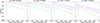 |
Fig. 10. Same as Fig. 9, but assuming a fixed spin value of 0.998 and considering different values for the accretion disc inclination (from left to right): i = 45° ,50° ,55°, and 60°. |
5. Returning radiation and corona optical depth predictions with kerrC
In order to ascertain the effect that returning radiation, along with the presence or absence of a corona, has on the observed polarisation properties of the source, we employed the general relativistic ray-tracing code kerrC (Krawczynski & Beheshtipour 2022; Krawczynski et al. 2022). The code operates under the prescription of a standard geometrically thin, optically thick accretion disc spanning from the ISCO to 100 gravitational radii and draws from a library of 68 040 BH, accretion flow, and corona configurations. Using the NICER and NuSTAR joint fit described in Sect. 3.1 we fixed the absorption, BH mass, distance, spin, mass accretion rate, and inclination to the values in Table 1 corresponding to Period 2. We used kerrC to simulate the polarisation of the source for the cases in which returning radiation is either disregarded or considered towards the total emission. The coronal optical depth τC is measured vertically from the accretion disc to the upper edge of the corona. A value of τC = 0 corresponds to a system where no coronal plasma is present and the emission consists only of direct emission from the disc and, optionally, of returning emission owing to space-time curvature without scattering in the corona. As the coronal optical depth increases, the total emission includes reflected emission from the disc onto the corona, which increases the PD (Schnittman & Krolik 2009).
In our predictions, we used a wedge-shaped corona with a temperature of 100 keV. The corona opening angle was 10°, the photospheric electron density was set to log10ne = 17.5, and the metallicity to AFe = 1.0 as per Krawczynski et al. (2022). We employed three different corona optical depths, τC = 0, 0.01, and 0.05, at the proposed inclination of 75°. In the case where returning radiation is neglected, the predicted PD increases with the presence of a corona: from 1.88% without a corona to 2.02% and 2.01% with corona optical depths of 0.01 and 0.05, respectively, in the 2–8 keV band. While these PDs are well within the confidence region of the observation, they fail to replicate the rise of PD with respect to energy shown in Fig. 4. For optical depths 0.0 and 0.01, the PD decreases by 0.69% and 0.32%, respectively, across the IXPE band. When the corona optical depth is 0.05, the PD only experiences a slight increase of 0.04%.
In the case where returning radiation is taken into consideration, the predicted PDs are 3.50%, 3.28%, and 3.43% for corona optical depths of 0.0, 0.01, and 0.05. The predicted 2–8 keV energy-averaged PD is higher than the observed PD, which may be attributed to the 6–8 keV PD being below the MDP. When returning radiation is considered, the PD increases from 1.54%, 1.60%, and 1.78% between 2 and 3 keV to 2.89%, 3.04%, and 3.59% in the 4.3–6.0 keV energy band in accordance to the observation. Our simulations with kerrC suggest that returning radiation is necessary to reproduce the IXPE polarisation results. Additionally, we tested a spin of a = 0.95 for the configurations with the highest energy average PD, namely for the case of returning radiation and a corona optical depths 0.0 and 0.05. For τC = 0.0, the PD is 1.18% between 2 and 3 keV and increases to 1.41% between 4.3 and 6.0 keV. For τC = 0.05, the PD increases from 1.15% to 1.42% in the same energy bands. A kerrC model of low spin fails to reproduce the data. A comprehensive examination of the source’s spectro-polarimetric characteristics and partial contributions of returning radiation using the kerrC code exceeds the scope of this study and will be addressed in a future work.
6. Conclusions
We performed an X-ray spectro-polarimetric observational campaign on the accreting low-mass X-ray binary BH system 4U 1957+115, with coverage by the IXPE, NICER, NuSTAR, and SRG missions. Our spectral analysis indicates that the source was in a soft state, characterised by a predominant thermal disc emission, with only a minor contribution from a Comptonised component and no clear reflection features. We observed a diminishing trend in the contribution of the hard X-ray tail during the observation period, with the initial NuSTAR data exhibiting the strongest power-law tail. Notably, this trend was not discernable from the IXPE and NICER data, highlighting that the Comptonisation component becomes relevant only above ∼10 keV and contributes only marginally in the IXPE energy range (2.3%, 1%, and 0.7% during the three NuSTAR observations). Our spectral fitting, which used a relativistic accretion disc emission model, strongly favours configurations characterised by large inclination angles and high spin values. By fixing the inclination, mass, and distance parameters to fiducial values, we estimate the BH spin to be 0.992 ± 0.003, which aligns with the literature values, considering the uncertainties (but see Sharma et al. 2021). The polarimetric observation of 4U 1957+115 revealed a time-averaged 2–8 keV PD of 1.9%±0.6% with a PA of  . The PA remains constant across different energy bins, while the PD shows a slight increase with energy, rising from ≈1.6% between 2 and 3 keV to ≈3.1% in the 4.3–6.0 keV energy band. The observed polarimetric data are consistent with theoretical predictions for thermal emission originating from an optically thick and geometrically thin disc with a Novikov-Thorne profile, assuming Chandrasekhar (1960) and Sobolev (1963) prescriptions for polarisation due to electron scattering in semi-infinite atmospheres. This agreement is achieved by accounting for the substantial contribution of self-irradiation. It is important to note that the inclusion of absorption effects could alternatively give rise to an increase in the PD with energy, mimicking the contribution of returning radiation (Ratheesh et al. 2024). The impact of absorption, however, is estimated to be negligible in the disc atmosphere of rapidly rotating BHs, because matter in the inner regions of the accretion disc is expected to be almost completely ionised due to the higher temperatures and lower densities of the plasma (Taverna et al. 2021). Additionally, due to the lack of spectral features, we can rule out any contribution of highly ionised gas along the line of sight Therefore, we regard the pure scattering atmosphere as a reasonable approximation to model our data. Our spectro-polarimetric analysis indicates that configurations with low BH spin values or low inclination angles are disfavoured within the standard Novikov-Thorne thin disc model, in agreement with the spectral analysis. In fact, such configurations struggle to explain the observed increase in PD with energy without requiring unphysically high PD values for the power-law component.
Available at https://heasarc.gsfc.nasa.gov/docs/ixpe/archive/
The NICER response file gain parameter values from the spectral analysis are 1.03 ± 0.01 for the slope and ( − 7.38 ± 0.26)×10−2 keV for the offset.
NICER calibration recommendations can be found at https://heasarc.gsfc.nasa.gov/docs/nicer/analysis_threads/cal-recommend/
Due to the strong degeneracy between the hardening factor and the BH spin parameter we further investigated if the high spin scenario depicted by the spectral fit remained consistent assuming different values for the hd parameter. When setting hd = 2 our analysis yielded a BH spin of  , with a χ2/d.o.f. of 979.5/951. On the other hand, when considering hd = 1.5, we obtained a lower limit for the BH spin of 0.997, with a χ2/d.o.f. of 973.9/951.
The IXPE response file gain parameter values from the spectral analysis are: DU1 slope 0.99 ± 0.01, offset ( − 1.52 ± 0.25)×10−2 keV; DU2 slope 0.98 ± 0.01, offset (2.23 ± 0.34)×10−2 keV; DU3 slope 0.99 ± 0.01, offset (1.46 ± 0.21)×10−2 keV.
Acknowledgments
The Imaging X-ray Polarimetry Explorer (IXPE) is a joint US and Italian mission. The US contribution is supported by the National Aeronautics and Space Administration (NASA) and led and managed by its Marshall Space Flight Center (MSFC), with industry partner Ball Aerospace (contract NNM15AA18C). The Italian contribution is supported by the Italian Space Agency (Agenzia Spaziale Italiana, ASI) through contract ASI-OHBI-2022-13-I.0, agreements ASI-INAF-2022-19-HH.0 and ASI-INFN-2017.13-H0, and its Space Science Data Center (SSDC) with agreements ASI-INAF-2022-14-HH.0 and ASI-INFN 2021-43-HH.0, and by the Istituto Nazionale di Astrofisica (INAF) and the Istituto Nazionale di Fisica Nucleare (INFN) in Italy. This research used data products provided by the IXPE Team (MSFC, SSDC, INAF, and INFN) and distributed with additional software tools by the High-Energy Astrophysics Science Archive Research Center (HEASARC), at NASA Goddard Space Flight Center (GSFC). M. Brigitte acknowledges the support from GAUK project No. 102323. N.R.C. and H.K. acknowledge support by NASA grants 80NSSC22K1291, 80NSSC23K1041, and 80NSSC20K0329. A.V. thanks the Academy of Finland grant 355672 for support. M.P. and P.-O.P. acknowledge financial support from the High Energy National Programme (PNHE) of the Scientific Research National center (CNRS) and from the french spatial agency (Centre National d’Études Spatiales, CNES). M.D., J.Pod., J.S. and V.K. thank for the support from the GACR project 21-06825X and the institutional support from RVO:67985815. I.L. was supported by the NASA Postdoctoral Program at the Marshall Space Flight Center, administered by Oak Ridge Associated Universities under contract with NASA. This research was also supported by the INAF grant 1.05.23.05.06: “Spin and Geometry in accreting X-ray binaries: The first multi frequency spectro-polarimetric campaign”.
References
- Arnaud, K. A. 1996, in Astronomical Data Analysis Software and Systems V, eds. G. H. Jacoby, & J. Barnes (San Francisco: Astron. Soc. Pac.), ASP Conf. Ser., 101, 17 [NASA ADS] [Google Scholar]
- Baldini, L., Bucciantini, N., Lalla, N. D., et al. 2022, SoftwareX, 19, 101194 [NASA ADS] [CrossRef] [Google Scholar]
- Barillier, E., Grinberg, V., Horn, D., et al. 2023, ApJ, 944, 165 [NASA ADS] [CrossRef] [Google Scholar]
- Bayless, A. J., Robinson, E. L., Mason, P. A., & Robertson, P. 2011, ApJ, 730, 43 [NASA ADS] [CrossRef] [Google Scholar]
- Chandrasekhar, S. 1960, Radiative Transfer (New York: Dover) [Google Scholar]
- Connors, P. A., & Stark, R. F. 1977, Nature, 269, 128 [Google Scholar]
- Connors, P. A., Piran, T., & Stark, R. F. 1980, ApJ, 235, 224 [Google Scholar]
- Connors, R. M. T., García, J. A., Dauser, T., et al. 2020, ApJ, 892, 47 [NASA ADS] [CrossRef] [Google Scholar]
- Connors, R. M. T., García, J. A., Tomsick, J., et al. 2021, ApJ, 909, 146 [NASA ADS] [CrossRef] [Google Scholar]
- Dauser, T., García, J. A., Joyce, A., et al. 2022, MNRAS, 514, 3965 [NASA ADS] [CrossRef] [Google Scholar]
- Dovčiak, M., Karas, V., & Matt, G. 2004, MNRAS, 355, 1005 [CrossRef] [Google Scholar]
- Dovčiak, M., Muleri, F., Goosmann, R. W., Karas, V., & Matt, G. 2008, MNRAS, 391, 32 [CrossRef] [Google Scholar]
- Draghis, P. A., Miller, J. M., Zoghbi, A., et al. 2023, ApJ, 946, 19 [NASA ADS] [CrossRef] [Google Scholar]
- Fabian, A. C., & Lasenby, A. N. 2019, arXiv e-prints [arXiv:1911.04305] [Google Scholar]
- Farr, W. M., Sravan, N., Cantrell, A., et al. 2011, ApJ, 741, 103 [NASA ADS] [CrossRef] [Google Scholar]
- Gaia Collaboration (Brown, A. G. A., et al.) 2021, A&A, 649, A1 [NASA ADS] [CrossRef] [EDP Sciences] [Google Scholar]
- Gendreau, K. C., Arzoumanian, Z., & Okajima, T. 2012, in Space Telescopes and Instrumentation 2012: Ultraviolet to Gamma Ray, eds. T. Takahashi, S. S. Murray, & J. W. A. den Herder, Proc. SPIE, 8443, 844313 [Google Scholar]
- Giacconi, R., Murray, S., Gursky, H., et al. 1974, ApJS, 27, 37 [NASA ADS] [CrossRef] [Google Scholar]
- Gomez, S., Mason, P. A., & Robinson, E. L. 2015, ApJ, 809, 9 [NASA ADS] [CrossRef] [Google Scholar]
- Hakala, P. J., Muhli, P., & Dubus, G. 1999, MNRAS, 306, 701 [NASA ADS] [CrossRef] [Google Scholar]
- Hakala, P., Muhli, P., & Charles, P. 2014, MNRAS, 444, 3802 [NASA ADS] [CrossRef] [Google Scholar]
- Harrison, F. A., Craig, W. W., Christensen, F. E., et al. 2013, ApJ, 770, 103 [Google Scholar]
- Kaastra, J. S., & Bleeker, J. A. M. 2016, A&A, 587, A151 [NASA ADS] [CrossRef] [EDP Sciences] [Google Scholar]
- Kato, S., Fukue, J., & Mineshige, S. 2008, Black-Hole Accretion Disks - Towards a New Paradigm (Kyoto: Kyoto Univ. Press) [Google Scholar]
- Krawczynski, H., & Beheshtipour, B. 2022, ApJ, 934, 4 [NASA ADS] [CrossRef] [Google Scholar]
- Krawczynski, H., Muleri, F., Dovčiak, M., et al. 2022, Science, 378, 650 [NASA ADS] [CrossRef] [Google Scholar]
- Lazar, H., Tomsick, J. A., Pike, S. N., et al. 2021, ApJ, 921, 155 [NASA ADS] [CrossRef] [Google Scholar]
- Li, L.-X., Zimmerman, E. R., Narayan, R., & McClintock, J. E. 2005, ApJS, 157, 335 [NASA ADS] [CrossRef] [Google Scholar]
- Loktev, V., Veledina, A., Poutanen, J., Nättilä, J., & Suleimanov, V. F. 2023, A&A, submitted [arXiv:2308.15159] [Google Scholar]
- Longa-Peña, P. 2015, Ph.D. Thesis, University of Warwick, UK [Google Scholar]
- Maccarone, T. J., Osler, A., Miller-Jones, J. C. A., et al. 2020, MNRAS, 498, L40 [NASA ADS] [CrossRef] [Google Scholar]
- Maitra, D., Miller, J. M., Reynolds, M. T., Reis, R., & Nowak, M. 2014, ApJ, 794, 85 [NASA ADS] [CrossRef] [Google Scholar]
- Margon, B., Thorstensen, J. R., & Bowyer, S. 1978, ApJ, 221, 907 [NASA ADS] [CrossRef] [Google Scholar]
- Mason, P. A., Robinson, E. L., Bayless, A. J., & Hakala, P. J. 2012, AJ, 144, 108 [NASA ADS] [CrossRef] [Google Scholar]
- Mikusincova, R., Dovciak, M., Bursa, M., et al. 2023, MNRAS, 519, 6138 [NASA ADS] [CrossRef] [Google Scholar]
- Miller-Jones, J. C. A., Bahramian, A., Orosz, J. A., et al. 2021, Science, 371, 1046 [Google Scholar]
- Novikov, I. D., & Thorne, K. S. 1973, in Black Holes (Les Astres Occlus) (New York: Gordon& Breach), 343 [Google Scholar]
- Nowak, M. A., & Wilms, J. 1999, ApJ, 522, 476 [NASA ADS] [CrossRef] [Google Scholar]
- Nowak, M. A., Juett, A., Homan, J., et al. 2008, ApJ, 689, 1199 [NASA ADS] [CrossRef] [Google Scholar]
- Nowak, M. A., Wilms, J., Pottschmidt, K., et al. 2012, ApJ, 744, 107 [NASA ADS] [CrossRef] [Google Scholar]
- Orosz, J. A., Steeghs, D., McClintock, J. E., et al. 2009, ApJ, 697, 573 [NASA ADS] [CrossRef] [Google Scholar]
- Orosz, J. A., Steiner, J. F., McClintock, J. E., et al. 2014, ApJ, 794, 154 [NASA ADS] [CrossRef] [Google Scholar]
- Özel, F., Psaltis, D., Narayan, R., & McClintock, J. E. 2010, ApJ, 725, 1918 [CrossRef] [Google Scholar]
- Parra, M., Petrucci, P. O., Bianchi, S., et al. 2024, A&A, 681, A49 [NASA ADS] [CrossRef] [EDP Sciences] [Google Scholar]
- Pavlinsky, M., Tkachenko, A., Levin, V., et al. 2021, A&A, 650, A42 [EDP Sciences] [Google Scholar]
- Piconcelli, E., Jimenez-Bailón, E., Guainazzi, M., et al. 2004, MNRAS, 351, 161 [Google Scholar]
- Podgorný, J., Marra, L., Muleri, F., et al. 2023, MNRAS, 526, 5964 [CrossRef] [Google Scholar]
- Ponti, G., Fender, R. P., Begelman, M. C., et al. 2012, MNRAS, 422, L11 [NASA ADS] [CrossRef] [Google Scholar]
- Poutanen, J., & Svensson, R. 1996, ApJ, 470, 249 [CrossRef] [Google Scholar]
- Ratheesh, A., Dovčiak, M., Krawczynski, H., et al. 2024, ApJ, 964, 77 [NASA ADS] [CrossRef] [Google Scholar]
- Remillard, R. A., Loewenstein, M., Steiner, J. F., et al. 2022, AJ, 163, 130 [NASA ADS] [CrossRef] [Google Scholar]
- Ricci, D., Israel, G. L., & Stella, L. 1995, A&A, 299, 731 [NASA ADS] [Google Scholar]
- Rodriguez Cavero, N., Marra, L., Krawczynski, H., et al. 2023, ApJ, 958, L8 [NASA ADS] [CrossRef] [Google Scholar]
- Russell, D. M., Miller-Jones, J. C. A., Maccarone, T. J., et al. 2011, ApJ, 739, L19 [NASA ADS] [CrossRef] [Google Scholar]
- Schnittman, J. D., & Krolik, J. H. 2009, ApJ, 701, 1175 [CrossRef] [Google Scholar]
- Schnittman, J. D., & Krolik, J. H. 2010, ApJ, 712, 908 [NASA ADS] [CrossRef] [Google Scholar]
- Sharma, P., Sharma, R., Jain, C., Dewangan, G. C., & Dutta, A. 2021, Res. Astron. Astrophys., 21, 214 [CrossRef] [Google Scholar]
- Shimura, T., & Takahara, F. 1995, ApJ, 445, 780 [Google Scholar]
- Sobolev, V. V. 1963, A treatise on Radiative Transfer (Princeton: Van Nostrand) [Google Scholar]
- Soffitta, P., Baldini, L., Bellazzini, R., et al. 2021, AJ, 162, 208 [CrossRef] [Google Scholar]
- Stark, R. F., & Connors, P. A. 1977, Nature, 266, 429 [NASA ADS] [CrossRef] [Google Scholar]
- Steiner, J. F., McClintock, J. E., Remillard, R. A., et al. 2010, ApJ, 718, L117 [Google Scholar]
- Sunyaev, R., Arefiev, V., Babyshkin, V., et al. 2021, A&A, 656, A132 [NASA ADS] [CrossRef] [EDP Sciences] [Google Scholar]
- Tanaka, Y., & Lewin, W. H. G. 1995, in X-ray Binaries, Cambridge Astrophysics Series, eds. W. H. G. Lewin, J. van Paradijs, & E. P. J. van den Heuvel (Cambridge: Cambridge University Press), 26, 126 [NASA ADS] [Google Scholar]
- Taverna, R., Zhang, W., Dovčiak, M., et al. 2020, MNRAS, 493, 4960 [NASA ADS] [CrossRef] [Google Scholar]
- Taverna, R., Marra, L., Bianchi, S., et al. 2021, MNRAS, 501, 3393 [NASA ADS] [Google Scholar]
- Thorstensen, J. R. 1987, ApJ, 312, 739 [NASA ADS] [CrossRef] [Google Scholar]
- Veledina, A., Muleri, F., Poutanen, J., et al. 2023, arXiv e-prints [arXiv:2303.01174] [Google Scholar]
- Weisskopf, M. C., Elsner, R. F., & O’Dell, S. L. 2010, in Space Telescopes and Instrumentation 2010: Ultraviolet to Gamma Ray, eds. M. Arnaud, S. S. Murray, & T. Takahashi, SPIE Conf. Ser., 7732, 77320E [NASA ADS] [CrossRef] [Google Scholar]
- Weisskopf, M. C., Soffitta, P., Baldini, L., et al. 2022, J. Astron. Telesc. Instrum. Syst., 8, 026002 [NASA ADS] [CrossRef] [Google Scholar]
- Wijnands, R., Miller, J. M., & van der Klis, M. 2002, MNRAS, 331, 60 [NASA ADS] [CrossRef] [Google Scholar]
- Wilms, J., Allen, A., & McCray, R. 2000, ApJ, 542, 914 [Google Scholar]
- Yao, Y., Nowak, M. A., Wang, Q. D., Schulz, N. S., & Canizares, C. R. 2008, ApJ, 672, L21 [Google Scholar]
- Yaqoob, T., Ebisawa, K., & Mitsuda, K. 1993, MNRAS, 264, 411 [NASA ADS] [CrossRef] [Google Scholar]
- Zhang, W., Dovčiak, M., Bursa, M., et al. 2022, MNRAS, 515, 2882 [CrossRef] [Google Scholar]
All Tables
Best-fitting parameters obtained in the spectral analysis of NICER and NuSTAR data during the three periods of observation.
All Figures
|
Fig. 1. Light curves of 4U 1957+115 as seen by NICER in the 0.3–12 keV energy band, NuSTAR in 3–20 keV, IXPE in 2–8 keV, and ART-XC in 4–12 keV. NuSTAR data coloured in blue, red, and green refer to the three epochs described in the spectral analysis and used in the spectra shown in Fig. 3. The vertical orange line shows the subdivision of the IXPE observation described in Sect. 3.2, and the dashed horizontal lines in the NICER and IXPE light curves indicate the mean values of the count rate. |
| In the text | |
|
Fig. 2. Time evolution of the hardness ratio from NICER, NuSTAR, IXPE, and ART-XC data as defined in the text. NuSTAR and NICER data coloured in blue, red, and green refer to the three epochs described in the spectral analysis and used in the spectra shown in Fig. 3. The vertical orange line shows the subdivision of the IXPE observation described in Sect. 3.2. |
| In the text | |
|
Fig. 3. NICER and NuSTAR spectra of 4U 1957+115. Top panel: unfolded spectra (i.e. the flux F(E)) for the best-fitting model described by Model 1 during Periods 1, 2, and 3, shown in red, blue, and green, respectively. The total model for each period, the contributions of the kerrbb and the powerlaw models are shown with the solid, dotted and dashed lines, respectively. Bottom panel: model minus data residuals in units of σ. |
| In the text | |
|
Fig. 4. Measured PD (left) and PA (right) of 4U 1957+115, shown with 1σ error bars. The shaded grey area in the PD-plot is an estimate of the MDP99, which shows a significant polarisation measurement from 2 keV up to 6 keV. |
| In the text | |
|
Fig. 5. Polar plot of the PD and PA, assuming the spectral best-fit model, in four energy bins: 2.0–3.0, 3.0–4.3, 4.3–6.0, and 6.0–8.0 keV. The shaded and unshaded regions show the 68% and 99.9% confidence areas, respectively, in the first three energy bins. The dashed line indicates the 99.9% confidence level upper limit in the fourth energy bin. |
| In the text | |
|
Fig. 6. PD (top) and PA (bottom) predicted by the kynbbrr model for the disc emission, assuming all system parameters are fixed at their respective best-fitting values (see Table 1). The different colours indicate different contributions of the returning radiation component, regulated by the albedo parameter. The vertical dashed lines highlight the 2–8 keV energy range. Here, the PA is defined with respect to the disc axis position angle χ0. |
| In the text | |
|
Fig. 7. Contour plot of the corona emission PD and the kynbbrr albedo parameter, which regulates the returning radiation contribution. Blue, red, and green lines indicate 68%, 90%, and 99% confidence levels for two parameters of interest, respectively, while the black cross indicates the best-fitting parameters. The dotted vertical line represents the assumed upper limit on the corona emission PD, as described in Sect. 3.3. |
| In the text | |
|
Fig. 8. PD (top row) and PA (bottom row) predicted by the kynbbrr model for the disc emission assuming different values for the BH spin and for the system inclination (from left to right): a = 0.5 and i = 75°, a = 0.96 and i = 75°, a = 0.998 and i = 75°, and a = 0.998 and i = 50°. The different colours indicate different contributions of the returning radiation component, regulated by the albedo parameter. The vertical dashed lines highlight the 2–8 keV energy range. Here, the PA is defined with respect to the disc axis position angle χ0. |
| In the text | |
|
Fig. 9. Contour plot of the corona emission PD and the kynbbrr albedo parameter, assuming four different spin values (from left to right): a = 0.95, 0.96, 0.97, and 0.998. The system inclination is assumed to be 75° in all cases. Blue, red and green lines indicate 68%, 90%, and 99% confidence levels for two parameters of interest, respectively, while the black cross indicates the best-fitting parameters. The dotted vertical line represents the assumed upper limit on the corona emission PD, as described in Sect. 3.3. |
| In the text | |
|
Fig. 10. Same as Fig. 9, but assuming a fixed spin value of 0.998 and considering different values for the accretion disc inclination (from left to right): i = 45° ,50° ,55°, and 60°. |
| In the text | |
Current usage metrics show cumulative count of Article Views (full-text article views including HTML views, PDF and ePub downloads, according to the available data) and Abstracts Views on Vision4Press platform.
Data correspond to usage on the plateform after 2015. The current usage metrics is available 48-96 hours after online publication and is updated daily on week days.
Initial download of the metrics may take a while.