| Issue |
A&A
Volume 692, December 2024
|
|
|---|---|---|
| Article Number | A123 | |
| Number of page(s) | 7 | |
| Section | Stellar structure and evolution | |
| DOI | https://doi.org/10.1051/0004-6361/202452642 | |
| Published online | 05 December 2024 | |
First spectropolarimetric observation of the neutron star low-mass X-ray binary GX 3+1
1
Dipartimento di Matematica e Fisica, Università degli Studi Roma Tre, via della Vasca Navale 84, I-00146 Roma, Italy
2
INAF – Osservatorio di Astrofisica e Scienza dello Spazio, Via P. Gobetti 101, 40129 Bologna, Italy
3
INAF – Istituto di Astrofisica e Planetologia Spaziali, Via del Fosso del Cavaliere 100, 00133 Roma, Italy
4
Department of Physics, McGill University, 3600 rue University, Montréal, QC H3A 2T8, Canada
5
Trottier Space Institute, McGill University, 3550 rue University, Montréal, QC H3A 2A7, Canada
6
Department of Physics and Astronomy, FI-20014 University of Turku, Finland
7
INAF Osservatorio Astronomico di Cagliari, via della Scienza 5 I-09047 Selargius (CA), Italy
8
NASA Marshall Space Flight Center, Huntsville, AL 35812, USA
9
MIT Kavli Institute for Astrophysics and Space Research, Massachusetts Institute of Technology, Cambridge, MA 02139, USA
⋆ Corresponding author; This email address is being protected from spambots. You need JavaScript enabled to view it.
Received:
17
October
2024
Accepted:
12
November
2024
Abstract
We report the first simultaneous X-ray spectropolarimetric observation of the bright atoll neutron star low-mass X-ray binary GX 3+1, performed by the Imaging X-ray Polarimetry Explorer (IXPE) joint with NICER and NuSTAR. The source does not exhibit significant polarization in the 2–8 keV energy band, with an upper limit of 1.3% at a 99% confidence level on the polarization degree. The observed spectra can be well described by a combination of thermal disk emission, the hard Comptonization component, and reflected photons off the accretion disk. In particular, from the broad Fe Kα line profile, we were able to determine the inclination of the system (i ≈ 36°), which is crucial for comparing the observed polarization with theoretical models. Both the spectral and polarization properties of GX 3+1 are consistent with those of other atoll sources observed by IXPE. Therefore, we may expect a similar geometrical configuration for the accreting system and the hot Comptonizing region. The low polarization is also consistent with the low inclination of the system.
Key words: polarization / X-rays: binaries / X-rays: individuals: GX 3+1
© The Authors 2024
 Open Access article, published by EDP Sciences, under the terms of the Creative Commons Attribution License (https://creativecommons.org/licenses/by/4.0), which permits unrestricted use, distribution, and reproduction in any medium, provided the original work is properly cited.
This article is published in open access under the Subscribe to Open model. This email address is being protected from spambots. You need JavaScript enabled to view it. to support open access publication.
1. Introduction
Weakly-magnetized neutron stars in low-mass X-ray binaries (NS-LMXBs) are among the brightest sources in the X-ray sky and are perfect laboratories for studying the properties of accretion in the strong gravity regime with X-ray polarimetry. Matter accretes onto the NS surface through Roche-lobe overflow, typically from a late main-sequence or evolved degenerate companion star. The surface of the NS stops the accretion flow, creating a boundary (BL) or spreading layer (SL) between the inner edge of the accretion disk and the NS, which extends to higher latitudes as the accretion rate increases (Inogamov & Sunyaev 1999; Popham & Sunyaev 2001; Suleimanov & Poutanen 2006).
According to their joint timing and spectral properties in the X-ray band, NS-LMXBs are traditionally divided into a few broad categories according to their tracks in the Hard-color/Soft-color diagrams (CCDs) or hardness-intensity diagrams (HIDs; Hasinger & van der Klis 1989; van der Klis 1989, 2006: Atolls (L ∼ 1036 erg s−1) show less extended and more compact tracks in a rounded single spot in the hard region of the CCD, termed the island state, or in a banana-shaped branch for bright Atolls (L = 1037 − 1038 erg s−1; van der Klis 1995); Z-sources (L > 1038 erg s−1) exhibit a wide Z-like three-branch pattern in the CCD (van der Klis 2006; Kuulkers et al. 1994; Migliari & Fender 2006). At lower luminosities, Atoll sources generally trace isolated patches on timescales from days to weeks, whereas the motion is faster at higher luminosities when they move along the banana branch, sometimes showing secular motion that does not influence the variability of the source (Migliari & Fender 2006).
X-ray spectra of NS-LMXBs are typically modeled with a thermal component dominating at lower energies (below 1–2 keV) plus a harder Comptonized emission. Thermal emission may be related to the direct emission of the accretion disk (Mitsuda et al. 1984, 1989) or of the NS surface, while hard emission is due to inverse Compton scattering of the soft photons by a hot electron plasma, whose geometric configuration and physical properties are still not clear. In addition, the accretion disk can reprocess the primary X-ray continuum, leading to a reflection component that usually includes fluorescent emission lines (Di Salvo et al. 2009; Miller et al. 2013; Mondal et al. 2017; Ludlam et al. 2019; Iaria et al. 2020; see also review by Ludlam 2024). X-ray polarimetry, along with timing and spectral observations, could be crucial for determining the geometry and physical characteristics of the system.
The Imaging X-ray Polarimetry Explorer (IXPE; Weisskopf et al. 2016, 2022), successfully launched on 2021 December 9, has introduced a powerful new instrument for studying the physical properties of various types of X-ray astronomical objects. IXPE features three X-ray telescopes that use polarization-sensitive imaging detectors (the gas-pixel detectors; Costa et al. 2001) to measure the Stokes parameters of the X-ray radiation, operating in the 2–8 keV energy range.
Being bright sources, IXPE has observed several NS-LMXBs so far (see also the review by Ursini et al. 2024b): out of the twelve NS-LMXBs observed so far (seven Z-sources, five Atolls, and two peculiar sources), Atolls are generally less polarized than Z-sources in the 2–8 keV range (Capitanio et al. 2023; Ursini et al. 2023a, 2024a; Di Marco et al. 2023a; Saade et al. 2024), but exhibit an increasing trend of the polarization degree with energy. The polarization signal in most observed NS-LMXBs is related to the hard component, characterized by a higher polarization compared to the soft thermal emission (Farinelli et al. 2023; Cocchi et al. 2023; Ursini et al. 2023a; La Monaca et al. 2024). In the majority of NS-LMXBs observed by IXPE, the polarization of the hard component seems to originate from the BL or SL, plus the contribution of reflection: these soft photons reflected off the accretion disk may significantly contribute to the polarization signal (Lapidus & Sunyaev 1985; Matt 1993), despite their relatively minor contribution to the overall flux. A peculiar behavior was observed for the ultracompact Atoll 4U 1820–303, which exhibited a rapid increase in polarization up to 10%±2% in the 7–8 keV band (Di Marco et al. 2023a), much higher than expected for typical BL or SL configurations (Gnarini et al. 2022; Capitanio et al. 2023; Ursini et al. 2023a; Farinelli et al. 2024; Bobrikova et al. 2024). Therefore, a different shape of the Comptonizing region or an additional contribution, for example from outflows, is required to explain this high polarization.
GX 3+1 is a persistent and bright Atoll discovered by Bowyer et al. (1965) and identified as an accreting NS in a LMXB system from the detection of Type I X-ray bursts with typical timescales of tens of seconds (Makishima et al. 1983; Kuulkers & van der Klis 2000; den Hartog et al. 2003; Chenevez et al. 2006) and exhibits superbursts of longer duration (up to hours) due to carbon burning (Kuulkers 2002). Assuming that type I X-ray bursts are Eddington limited, the estimated upper limit to the source distance is ∼6.5 kpc (Galloway et al. 2008), consistent with the results obtained from a double peak photospheric radius expansion burst (Kuulkers & van der Klis 2000). The near-infrared (NIR) counterpart to GX 3+1 was discovered by van den Berg et al. (2014) as a star with 15.8 ± 0.1 mag, suggesting that the donor star may not be a late-type giant with the NIR dominated by the emission of the outer accretion disk. GX 3+1 is among the brightest persistent Atoll sources associated with the bulge component of the Milky Way. These sources are typically characterized by high X-ray luminosity (1037 − 1038 erg s−1), with moderate and irregular flux variations. Similarly to the bright atolls GX 9+1 and GX 9+9, GX 3+1 exhibits strong long-term X-ray flux modulations, with a timescale of ∼6 yr (Kotze & Charles 2010; Durant et al. 2010), likely due to variations in the mass-transfer rate. Moreover, this NS-LMXB was observed only in its banana branch (Lewin et al. 1987; Hasinger & van der Klis 1989; Asai et al. 1993; Pintore et al. 2015; Thomas et al. 2023), without any evidence of island state in its CCD or HID.
The X-ray spectrum of GX 3+1 can be well described by the combination of a soft thermal component, most likely related to the accretion disk, plus a Comptonized component due to the hot electron population in the corona (Oosterbroek et al. 2001; Mainardi et al. 2010; Seifina & Titarchuk 2012; Piraino et al. 2012; Pintore et al. 2015; Ludlam et al. 2019). Several Kα broad emission lines of Ar, Ca, and Fe were also detected in GX 3+1 spectra (Oosterbroek et al. 2001; Piraino et al. 2012). These features arise from the reprocessing of X-ray photons illuminating the accretion disk. In particular, the location of the inner disk radius and the inclination of the system can be estimated from the relativistically broadened Fe Kα line profile: from XMM-Newton and INTEGRAL observations, the inclination is ∼35° with the inner edge of the accretion disk located at ∼10 Rg (where Rg = GM/c2; Pintore et al. 2015), while it appears to be closer to the innermost stable circular orbit (ISCO) in a NuSTAR observation, with an inclination of 27 ° −31° (Ludlam et al. 2019).
The paper is structured as follows. In Sect. 2, we describe the IXPE, NuSTAR, and NICER observations and data reduction. In Sect. 3, we present the X-ray spectropolarimetric analysis. Finally, in Sects. 4 and 5, we discuss the results and the main conclusions.
2. Observations and data reduction
2.1. IXPE
IXPE observed GX 3+1 from 2024 August 16 07:26:28 UT to August 17 08:24:32 UT for a total exposure time of 47.7 ks (see Table 1). We extracted time-resolved spectral and polarimetric data files for each detector unit (DU) with the standard FTOOLS procedure1 (HEASoft v6.33; NASA High Energy Astrophysics Science Archive Research Center 2014) and the latest available calibration files (CALDB v.20240125). The data analysis was performed considering the weighted analysis method presented in Di Marco et al. (2022) with the parameter stokes=Neff in XSELECT (see also Baldini et al. 2022). We extracted the source spectra and light curves from a circular region of 120″ radius centered on the source, with radius derived through an iterative procedure to maximize the signal-to-noise ratio (S/N) in the 2–8 keV band, similar to the approach described in Piconcelli et al. (2004). The background was extracted from an annular region centered on the source with an inner and outer radius of 180″ and 240″ respectively, but it was not subtracted during the analysis, following the prescription by Di Marco et al. (2023b) for bright sources. However, we verified that the subtraction of the background has a minimal impact on the results, particularly on the polarimetric measurements. The ancillary response file (ARF) and modulation response file (MRF) for each DU was generated using the ixpecalcarf task, considering the same extraction radius used for the source region.
Log of the observations of GX 3+1.
2.2. NuSTAR
The Nuclear Spectroscopic Telescope Array (NuSTAR; Harrison et al. 2013) observed GX 3+1 with its X-ray telescopes on focal plane module A (FPMA) and B (FPMB) from 2024 August 16 16:56:09 UT to August 17 22:56:09 UT for a net exposure time of 34.3 ks (see Table 1). We extracted clean event files using the latest calibration files (CALDB v.20240812) and the standard nupipeline task of the NuSTAR Data Analysis Software (NUSTARDAS v.2.1.4) with the keyword statusexpr="(STATUS==b0000xxx00xxxx000)&&(SHIELD= = 0)" due to the source brightness (> 100 counts s−1). The source spectrum and light curves for each FPM were extracted using the nuproducts task from a circular region centered on the source with 120″ radius. The extraction radii of the source regions were calculated with the same procedure of maximization of the S/N used for IXPE data reduction (see also Piconcelli et al. 2004; Marinucci et al. 2022; Ursini et al. 2023b). Since the background is not negligible at all energies, we performed background subtraction. For both FPMs, the background was extracted from a circular region with 60″ radius sufficiently far from the source. For the spectropolarimetric analysis, we considered the NuSTAR data in the 3–25 keV range, since the background starts dominating above 25 keV. The spectra were also rebinned using the standard ftgrouppha task, with the optimal binning algorithm by Kaastra & Bleeker (2016) plus a minimum S/N of 3 per grouped bin. Type-I X-ray bursts were not detected in the light curves. No quasi-periodic oscillations were identified with the NuSTAR data. During the joint spectropolarimetric analysis, we only considered the NuSTAR data that were simultaneous with the IXPE observation.
2.3. NICER
The Neutron Star Interior Composition Explorer (NICER; Gendreau et al. 2016) observed GX 3+1 from 2024 August 16 15:35:51 UT to August 17 00:56:40 UT in different snapshots for a total exposure time of 1.2 ks (see Table 1). The calibrated and cleaned files were processed using the standard nicerl2 task of the NICER Data Analysis Software (NICERDAS v.13) together with the latest calibration files (CALDB v.20240206). The spectra and light curves were then obtained with the nicerl3-spec and nicerl3-lc commands, while the background was computed using the SCORPEON2 model. Due to their short duration, it is not possible to build a complete CCD or HID from the NICER observations. Neither Type-I X-ray bursts nor quasi-periodic oscillations were identified in the NICER data. The NICER data were considered in the 1–10 keV band. During spectropolarimetric analysis (Sect. 3), we found some significant residuals in the NICER energy spectra below 2–2.5 keV (Miller et al. 2018; Strohmayer et al. 2018), due to spectral features not included in the NICER ancillary response file (ARF). We add a multiplicative absorption edge (edge) with threshold energies of 1.81 ± 0.02 and a Gaussian component (gaussian) at 1.7 keV with a line width of 0.06 ± 0.01 keV.
3. Data analysis
3.1. Timing properties
The light curves obtained with IXPE, NuSTAR, and NICER are shown in Fig. 1, using time bins of 200 s for IXPE and NuSTAR, and 50 s for NICER. Some significant variations in the observed flux can be noticed for all three observatories, with small drops in the observed count rate. Despite the fact that the IXPE hardness ratio (HR: 5–8 keV/3–5 keV) remains quite constant throughout the observation, both NuSTAR and NICER data exhibit some variability: in particular, GX 3+1 moves along the CCD (Fig. 2) tracing part of the banana branch. The soft color is defined as the ratio of the counts in the 6–10/3–6 keV band, whereas the hard color as the ratio in the 10–20/6–10 keV energy range. Therefore, we divided the NuSTAR observation based on its hard color: when the hard color is less than 0.27, the source remains in the lower part of the CCD in the lower banana state (LB; red box in Fig. 2), while, when both the hard and soft colors increase, the source moves toward the upper banana branch (UB; purple box in Fig. 2). The gray regions in Fig. 1 correspond to the time intervals during which the source moves along the UB branch. The same time intervals were then used to extract and filter in time for the IXPE and NICER observations.
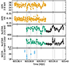 |
Fig. 1. IXPE, NuSTAR, and NICER light curves of GX 3+1 (count s−1). The second panel shows the IXPE hardness ratio (5–8 keV/3–5 keV). The fourth panel shows the NuSTAR hard color (10–20 keV/6–10 keV). Empty black circles denote the NuSTAR points that are not simultaneous with the IXPE observation. The gray regions correspond to the time intervals during which the source moves in the UB branch. For IXPE and NuSTAR, we considered time bins of 200 s, whereas for NICER we opted for 50 s bins. |
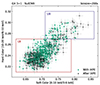 |
Fig. 2. NuSTAR CCD of GX 3+1. The soft and hard colors are defined as the ratio of the counts in the 6–10/3–6 keV and 10–20/6–10 keV bands, respectively. Empty black circles denote the NuSTAR points not simultaneous with IXPE observation. The red and purple boxes correspond to the LB and UB region. Each bin corresponds to 200 s. |
3.2. Spectral analysis
We performed a joint fit of the IXPE, NICER, and NuSTAR spectra during the LB and UB states with XSPEC (Arnaud 1996). We included energy-independent cross-calibration multiplicative factors for each IXPE DU, each NuSTAR FPM, and the NICER spectra. Then, we included the TBabs model with vern cross-section (Verner et al. 1996) and wilm abundances (Wilms et al. 2000) to take into account interstellar absorption, leaving the hydrogen column density NH free to vary. The best-fit value obtained (2.41 × 1022 cm−2) is consistent with that obtained by Ludlam et al. (2019). The primary continuum is modeled with two components: a disk multi-temperature blackbody (diskbb; Mitsuda et al. 1984) dominating at lower energies plus a Comptonized blackbody emission using the convolution model thcomp (Zdziarski et al. 2020) applied to the bbodyrad component. The covering factor f of thcomp is related to the fraction of Comptonized photons and results to be > 0.95, with best-fit value of 0.99. Therefore, we fixed it to its best-fit value to improve the fit statistic and better constrain the other parameters of thcomp. The physical parameters of diskbb and thcomp*bbodyrad are considered separately between the two spectral states. We noticed some residuals in the NICER and NuSTAR data, suggesting the presence of a strong iron Kα line (see the zoomed plot in Figs. 3 and 4) and a reflection component. Therefore, we added the reflection component to the model using relxillNS. The relxill models reproduce the relativistic reflection component from the innermost regions of the accretion disk (García et al. 2014; Dauser et al. 2014). In particular, relxillNS considers a single-temperature blackbody spectrum that illuminates the surface of the accretion disk at 45°, which could physically originate from the emission of the NS surface or the spreading layer. The temperature of the seed photons of relxillNS is linked to the black body temperature of bbodyrad of each spectral state. We fixed the number density at log ne/cm−3 = 16.5, since the fit is not very sensitive to this parameter. This value is consistent with the results found by Ludlam et al. (2019) and with the inner region of standard accretion disks (García et al. 2016; Ludlam et al. 2022). Moreover, we also fixed the emissivity index qem = 2.8 to the same value obtained by Ludlam et al. (2019), and the outer disk radius Rout = 1000 Rg, as the fit is not able to constrain these parameters. For a standard NS, the dimensionless spin a can be derived using the spin period P as a = 0.47/P(ms) (Braje et al. 2000). In particular, typical NSs in LMXBs are characterized by spin periods between 2 and 5 ms (Patruno et al. 2017; Di Salvo et al. 2024); therefore, the dimensionless spin can be fixed at a = 0.1. We left the inclination of the system, the inner disk radius (in units of the ISCO), the ionization parameter ξ, the iron abundance AFe and the normalization Nr free to vary. Since the best-fit values of all these parameters were very similar between the LB and UB spectra, we linked all the relxillNS parameters of the two spectral states to improve constraints on the results and we left only the two normalizations Nr separate.
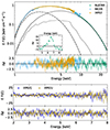 |
Fig. 3. Deconvolved IXPE (2–8 keV), NuSTAR (3–25 keV), NICER (1–10 keV) spectra (top panels), and IXPE Q and U Stokes spectra (bottom panels), with the best-fit model during the LB state and residuals in units of σ. We added the residuals without including the reflection components in the zoomed plot, highlighting the Fe Kα line profile. The best-fit model includes diskbb (dash-dotted lines), thcomp*bbodyrad (dashed lines), and relxillNS (dotted lines). |
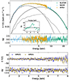 |
Fig. 4. Deconvolved IXPE (2–8 keV), NuSTAR (3–25 keV), NICER (1–10 keV) spectra (top panels), and IXPE Q and U Stokes spectra (bottom panels), with the best-fit model during the UB state and residuals in units of σ. We added the residuals without including the reflection components in the zoomed plot, highlighting the Fe Kα line profile. The best-fit model includes diskbb (dash-dotted lines), thcomp*bbodyrad (dashed lines), and relxillNS (dotted lines). |
The best-fit is obtained considering the following spectral model:
TBabs*(diskbb + thcomp*bbodyrad + relxillNS),
which is capable of providing excellent fits to the IXPE+NuSTAR+NICER spectra. The best-fit values for each parameter are reported in Table 2, while the spectra are represented in Figs. 3 and 4. The physical properties of both the disk and Comptonized components can be well constrained for both spectral states: the diskbb and bbodyrad temperature increase as the source moves from the LB to the UB state, while the best-fit values for the electron temperature kTe and optical depth τ of the Comptonizing region remain quite stable, differently from other Atoll sources, such as 4U 1728–34 (Tarana et al. 2011). The inclination i of the system can be well constrained from the reflection component, suggesting that the inclination is about 36°, while only an upper limit of 1.4 RISCO is obtained for the inner edge of the accretion disk. The ionization parameter ξ and the iron abundance AFe can also be obtained from the best-fit model with good precision.
Best-fitting model parameters of the fits to GX 3+1 IXPE+NuSTAR+NICER spectra.
The parameters obtained from the best-fit models are typical for bright atoll NS-LMXBs in the soft state. The apparent inner disk radius Rin and the radius of the black body photon-emitting region Rbb can be computed from the normalizations of diskbb and bbodyrad assuming a 6.5 kpc distance (Galloway et al. 2008) and that all seed photons of bbodyrad are Comptonized, which corresponds to f = 1. We found that the black body-emitting region has an equivalent spherical radius of ∼8 km during the LB state and it decreases up to ∼5.5 km during the UB intervals, consistent with seed photons originating in a region consistent with the spreading layer. From diskbb, the inner disk radius results to be close to  km, which is consistent with the upper limit derived from the reflection component using relxillNS.
3.3. Polarimetric analysis
To estimate polarization in the 2–8 keV band of GX 3+1, we first performed a polarimetric analysis of the entire IXPE observation using IXPEOBSSIM (v.31.0.1; Baldini et al. 2022), with the latest available calibration file (v.13.20240701). The normalized Stokes parameters measured by IXPE obtained using the PCUBE task of IXPEOBSSIM are shown in Fig. 5 for each DU, with the minimum detectable polarization (MDP) at the 99% level. The spectropolarimetric fitting procedure is performed with XSPEC by applying polconst to the best-fit models. No significant detection is obtained in the 2–8 keV band, with an upper limit to the polarization degree of 1.3% at the 99% confidence level for a single parameter of interest, which is independent of the value of the polarization angle. In Table 3 we report the polarization degree and angle measured in different energy bins obtained with XSPEC (Arnaud 1996), and the corresponding upper limits. The two-dimensional polarization contours in the full 2–8 keV band obtained with XSPEC are represented in Fig. 6. We tried also to separate the full IXPE band considering energy bins of 1 or 2 keV, but without any significant detection of the polarization in the considered energy range. Therefore, we did not find any evident trend of the polarization with energy. We also analyzed the polarimetric data for each GTI: during the time intervals with lower hard color, the polarization degree is < 1.4%, while when the soft and hard color increases, the upper limit of the polarization degree is 2.3%. Even by separating the data by hard color, we were not able to detect any significant evolution with energy. All results are consistent between the PCUBE task and the fitting procedure with XSPEC.
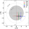 |
Fig. 5. Normalized Stokes q (Q/I) and u (U/I) parameters in the 2–8 keV band obtained with the PCUBE algorithm of IXPEOBSSIM (Baldini et al. 2022), for the three IXPE DUs and their combination. The gray-filled circle corresponds to the 99% MDP. |
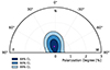 |
Fig. 6. Contour plots of the PD and PA at the 68%, 90%, and 99% confidence levels, in the 2–8 keV energy bands obtained with XSPEC. |
Polarization measured with XSPEC.
4. Discussion
The systematic effects on the derived polarization are expected to be minimized by the overlap of the energy range between IXPE and NuSTAR+NICER. Due to the limited band-pass of IXPE and the undetected polarization in the 2–8 keV energy band, it is difficult to estimate the polarization degree and angle for each spectral component. In particular, the Comptonization and reflection components exhibit similar spectral shapes, also peaking at similar energies. Therefore, we need some theoretical assumptions to find an estimate of the polarization of the different components.
We performed the spectropolarimetric fitting procedure by applying polconst to each spectral component:
TBabs*(polconst(d)*diskbb + polconst(r)
*relxillNS + polconst(c)*thcomp*bbodyrad).
During the analysis, we fixed all spectral parameters to their best-fit values (see Table 2), except for the cross-calibration constants, and left only the polconst polarization degree and angle free to vary. The results are reported in Table 4. As a first attempt, we tried to estimate the polarization of each spectral component assuming that only one is polarized and the other two have zero polarization (see Table 4). The only component for which we were able to constrain (at the 90% confidence level) the polarimetric contribution is diskbb, with 1.7%±1.4% PD, while only upper limits were obtained for Comptonization (< 2.6%, at the 99% confidence level) and reflection (< 8.1%, at the 99% confidence level). In all three cases, the fit results were acceptable with χ2/d.o.f. = 1.05. Although the results are perfectly consistent with the theoretical predictions for a semi-infinite plane-parallel atmosphere (Chandrasekhar 1960) for the disk component and with a typical spreading layer geometry for Comptonization (Gnarini et al. 2022; Ursini et al. 2023a; Farinelli et al. 2024; Bobrikova et al. 2024), the upper limit on the reflection polarization seems to be rather stringent. Reflected photons are expected to be highly polarized (Matt 1993; Poutanen et al. 1996) and can contribute significantly to the polarization signal even if their fraction with respect to the total flux is relatively low. For GX 3+1, the contribution of reflection to the total flux in the 2–8 keV energy range is quite high (≈15%). The resulting upper limit is slightly lower than the theoretical previsions for reflected radiation. We also tried to fix the disk PD to the classical value obtained by Chandrasekhar (1960) and the PD of the Comptonization component to 0.5% (see Table 4), a reasonable value for a spreading layer configuration observed at 36°. The PA of diskbb is fixed to be orthogonal to that of the reflected and Comptonized photons. With these assumptions, the fit does not improve while the upper limit slightly decreases (< 7.8% at the 99% confidence level). We also tried a different scenario in which the reflection is highly polarized as expected, with PD fixed at 10% (Matt 1993), while the polarization of thcomp*bbodyrad is left free to vary. The PD of diskbb is set again to the results obtained by Chandrasekhar (1960) for i ≈ 36°, polarized orthogonally with respect to the other two components. We obtained only an upper limit of 0.7% (at the 99% confidence level) for the PD of the Comptonized component, suggesting a spherical or a spreading layer-like geometry of the Comptonizing region (Gnarini et al. 2022; Farinelli et al. 2024; Bobrikova et al. 2024).
Polarization degree and angle of each spectral component for different scenarios.
5. Conclusions
We report the results of the first spectropolarimetric observation of the bright atoll NS-LMXB GX 3+1 performed with IXPE, with joint NICER and NuSTAR observations. Only an upper limit of 1.3% (at the 99% confidence level) can be derived from the IXPE data. The source was found in the banana branch, mainly on the lower part but moving towards the upper branch for short time intervals. The spectral properties remain quite stable during the motion along the banana branch: the spectra are well fitted with a two-component model, that is, disk plus Comptonized emission, with the addition of the reflected photons to remove some residuals at high energies and in the 6–7 keV energy range. From the reflection component, we were able to obtain an upper limit on the position of the inner edge of the accretion disk (Rin ≲ 1.5 RISCO) and to estimate the inclination of the system (i ≈ 36°). Therefore, the low polarization signal can be mainly due to the inclination, since more face-on systems are expected to be less polarized (Chandrasekhar 1960; Gnarini et al. 2022; Farinelli et al. 2024). Because we obtained only an upper limit on the polarization, we were not able to constrain the polarimetric properties of the different spectral components. However, we found a quite stringent upper limit for the PD of the reflection component: differently from other NS-LMXBs observed by IXPE, considering the observed photon flux ratios derived from the spectra, the reflected photons are expected to be less polarized (up to ≈8%); otherwise we would have obtained a polarization detection if not in the entire 2–8 keV band at least in some energy ranges. The upper limits on the disk and Comptonization component are still consistent with the theoretical expectation for a system with a standard accretion disk and a spreading layer-like geometry of the Comptonizing region.
Acknowledgments
The Imaging X-ray Polarimetry Explorer (IXPE) is a joint US and Italian mission. The US contribution is supported by the National Aeronautics and Space Administration (NASA) and led and managed by its Marshall Space Flight Center (MSFC). AG, SB, FC, SF, GM, AT, and FU acknowledge financial support by the Italian Space Agency (Agenzia Spaziale Italiana, ASI) through the contract ASI-INAF-2022-19-HH.0. This research was also supported by the Istituto Nazionale di Astrofisica (INAF) grant 1.05.23.05.06: “Spin and Geometry in accreting X-ray binaries: The first multi frequency spectro-polarimetric campaign”. SF has been supported by the project PRIN 2022 – 2022LWPEXW – “An X-ray view of compact objects in polarized light”, CUP C53D23001180006. AB acknowledges support from the Finnish Cultural Foundation grant 00240328. JP thanks the Academy of Finland grant 333112 for support. M.N. is a Fonds de Recherche du Quebec – Nature et Technologies (FRQNT) postdoctoral fellow. This research used data products and software provided by the IXPE, the NICER and NuSTAR teams and distributed with additional software tools by the High-Energy Astrophysics Science Archive Research Center (HEASARC), at NASA Goddard Space Flight Center (GSFC).
References
- Arnaud, K. A. 1996, ASP Conf. Ser., 101, 17 [Google Scholar]
- Asai, K., Dotani, T., Nagase, F., et al. 1993, PASJ, 45, 801 [NASA ADS] [Google Scholar]
- Baldini, L., Bucciantini, N., Lalla, N. D., et al. 2022, SoftwareX, 19, 101194 [NASA ADS] [CrossRef] [Google Scholar]
- Bobrikova, A., Poutanen, J., & Loktev, V. 2024, A&A, submitted [arXiv:2409.16023] [Google Scholar]
- Bowyer, S., Byram, E. T., Chubb, T. A., & Friedman, H. 1965, Science, 147, 394 [NASA ADS] [CrossRef] [Google Scholar]
- Braje, T. M., Romani, R. W., & Rauch, K. P. 2000, ApJ, 531, 447 [Google Scholar]
- Capitanio, F., Fabiani, S., Gnarini, A., et al. 2023, ApJ, 943, 129 [NASA ADS] [CrossRef] [Google Scholar]
- Chandrasekhar, S. 1960, Radiative Transfer (New York: Dover Publications) [Google Scholar]
- Chenevez, J., Falanga, M., Brandt, S., et al. 2006, A&A, 449, L5 [NASA ADS] [CrossRef] [EDP Sciences] [Google Scholar]
- Cocchi, M., Gnarini, A., Fabiani, S., et al. 2023, A&A, 674, L10 [NASA ADS] [CrossRef] [EDP Sciences] [Google Scholar]
- Costa, E., Soffitta, P., Bellazzini, R., et al. 2001, Nature, 411, 662 [NASA ADS] [CrossRef] [Google Scholar]
- Dauser, T., Garcia, J., Parker, M. L., Fabian, A. C., & Wilms, J. 2014, MNRAS, 444, L100 [Google Scholar]
- den Hartog, P. R., in’t Zand, J. J. M., Kuulkers, E., et al. 2003, A&A, 400, 633 [NASA ADS] [CrossRef] [EDP Sciences] [Google Scholar]
- Di Marco, A., Costa, E., Muleri, F., et al. 2022, AJ, 163, 170 [NASA ADS] [CrossRef] [Google Scholar]
- Di Marco, A., La Monaca, F., Poutanen, J., et al. 2023a, ApJ, 953, L22 [NASA ADS] [CrossRef] [Google Scholar]
- Di Marco, A., Soffitta, P., Costa, E., et al. 2023b, AJ, 165, 143 [CrossRef] [Google Scholar]
- Di Salvo, T., D’Aí, A., Iaria, R., et al. 2009, MNRAS, 398, 2022 [NASA ADS] [CrossRef] [Google Scholar]
- Di Salvo, T., Papitto, A., Marino, A., Iaria, R., & Burderi, L. 2024, in Handbook of X-ray and Gamma-ray Astrophysics, eds. C. Bambi, & A. Santangelo (Singapore: Springer), 4031 [CrossRef] [Google Scholar]
- Durant, M., Cornelisse, R., Remillard, R., & Levine, A. 2010, MNRAS, 401, 355 [NASA ADS] [CrossRef] [Google Scholar]
- Farinelli, R., Fabiani, S., Poutanen, J., et al. 2023, MNRAS, 519, 3681 [NASA ADS] [CrossRef] [Google Scholar]
- Farinelli, R., Waghmare, A., Ducci, L., & Santangelo, A. 2024, A&A, 684, A62 [NASA ADS] [CrossRef] [EDP Sciences] [Google Scholar]
- Galloway, D. K., Muno, M. P., Hartman, J. M., Psaltis, D., & Chakrabarty, D. 2008, ApJS, 179, 360 [NASA ADS] [CrossRef] [Google Scholar]
- García, J., Dauser, T., Lohfink, A., et al. 2014, ApJ, 782, 76 [Google Scholar]
- García, J. A., Fabian, A. C., Kallman, T. R., et al. 2016, MNRAS, 462, 751 [Google Scholar]
- Gendreau, K. C., Arzoumanian, Z., Adkins, P. W., et al. 2016, Proc SPIE, 9905, 99051H [NASA ADS] [CrossRef] [Google Scholar]
- Gnarini, A., Ursini, F., Matt, G., et al. 2022, MNRAS, 514, 2561 [NASA ADS] [CrossRef] [Google Scholar]
- Harrison, F. A., Craig, W. W., Christensen, F. E., et al. 2013, ApJ, 770, 103 [Google Scholar]
- Hasinger, G., & van der Klis, M. 1989, A&A, 225, 79 [NASA ADS] [Google Scholar]
- Iaria, R., Mazzola, S. M., Di Salvo, T., et al. 2020, A&A, 635, A209 [NASA ADS] [CrossRef] [EDP Sciences] [Google Scholar]
- Inogamov, N. A., & Sunyaev, R. A. 1999, Astron. Lett., 25, 269 [NASA ADS] [Google Scholar]
- Kaastra, J. S., & Bleeker, J. A. M. 2016, A&A, 587, A151 [NASA ADS] [CrossRef] [EDP Sciences] [Google Scholar]
- Kotze, M. M., & Charles, P. A. 2010, MNRAS, 402, L16 [NASA ADS] [Google Scholar]
- Kuulkers, E. 2002, A&A, 383, L5 [NASA ADS] [CrossRef] [EDP Sciences] [Google Scholar]
- Kuulkers, E., & van der Klis, M. 2000, A&A, 356, L45 [NASA ADS] [Google Scholar]
- Kuulkers, E., van der Klis, M., Oosterbroek, T., et al. 1994, A&A, 289, 795 [NASA ADS] [Google Scholar]
- La Monaca, F., Di Marco, A., Poutanen, J., et al. 2024, ApJ, 960, L11 [NASA ADS] [CrossRef] [Google Scholar]
- Lapidus, I. I., & Sunyaev, R. A. 1985, MNRAS, 217, 291 [NASA ADS] [CrossRef] [Google Scholar]
- Lewin, W. H. G., van Paradijs, J., Hasinger, G., et al. 1987, MNRAS, 226, 383 [NASA ADS] [CrossRef] [Google Scholar]
- Ludlam, R. M. 2024, Ap&SS, 369, 16 [NASA ADS] [CrossRef] [Google Scholar]
- Ludlam, R. M., Miller, J. M., Barret, D., et al. 2019, ApJ, 873, 99 [Google Scholar]
- Ludlam, R. M., Cackett, E. M., García, J. A., et al. 2022, ApJ, 927, 112 [NASA ADS] [CrossRef] [Google Scholar]
- Mainardi, L. I., Paizis, A., Farinelli, R., et al. 2010, A&A, 512, A57 [NASA ADS] [CrossRef] [EDP Sciences] [Google Scholar]
- Makishima, K., Mitsuda, K., Inoue, H., et al. 1983, ApJ, 267, 310 [NASA ADS] [CrossRef] [Google Scholar]
- Marinucci, A., Muleri, F., Dovciak, M., et al. 2022, MNRAS, 516, 5907 [NASA ADS] [CrossRef] [Google Scholar]
- Matt, G. 1993, MNRAS, 260, 663 [NASA ADS] [CrossRef] [Google Scholar]
- Migliari, S., & Fender, R. P. 2006, MNRAS, 366, 79 [CrossRef] [Google Scholar]
- Miller, J. M., Parker, M. L., Fuerst, F., et al. 2013, ApJ, 779, L2 [NASA ADS] [CrossRef] [Google Scholar]
- Miller, J. M., Gendreau, K., Ludlam, R. M., et al. 2018, ApJ, 860, L28 [NASA ADS] [CrossRef] [Google Scholar]
- Mitsuda, K., Inoue, H., Koyama, K., et al. 1984, PASJ, 36, 741 [NASA ADS] [Google Scholar]
- Mitsuda, K., Inoue, H., Nakamura, N., & Tanaka, Y. 1989, PASJ, 41, 97 [NASA ADS] [Google Scholar]
- Mondal, A. S., Pahari, M., Dewangan, G. C., Misra, R., & Raychaudhuri, B. 2017, MNRAS, 466, 4991 [NASA ADS] [Google Scholar]
- NASA High Energy Astrophysics Science Archive Research Center, 2014, HEAsoft: Unified Release of FTOOLS and XANADU, Astrophysics Source Code Library [record ascl:1408.004] [Google Scholar]
- Oosterbroek, T., Barret, D., Guainazzi, M., & Ford, E. C. 2001, A&A, 366, 138 [NASA ADS] [CrossRef] [EDP Sciences] [Google Scholar]
- Patruno, A., Haskell, B., & Andersson, N. 2017, ApJ, 850, 106 [NASA ADS] [CrossRef] [Google Scholar]
- Piconcelli, E., Jimenez-Bailón, E., Guainazzi, M., et al. 2004, MNRAS, 351, 161 [Google Scholar]
- Pintore, F., Di Salvo, T., Bozzo, E., et al. 2015, MNRAS, 450, 2016 [NASA ADS] [CrossRef] [Google Scholar]
- Piraino, S., Santangelo, A., Kaaret, P., et al. 2012, A&A, 542, L27 [NASA ADS] [CrossRef] [EDP Sciences] [Google Scholar]
- Popham, R., & Sunyaev, R. 2001, ApJ, 547, 355 [NASA ADS] [CrossRef] [Google Scholar]
- Poutanen, J., Nagendra, K. N., & Svensson, R. 1996, MNRAS, 283, 892 [NASA ADS] [CrossRef] [Google Scholar]
- Saade, M. L., Kaaret, P., Gnarini, A., et al. 2024, ApJ, 963, 133 [NASA ADS] [CrossRef] [Google Scholar]
- Seifina, E., & Titarchuk, L. 2012, ApJ, 747, 99 [NASA ADS] [CrossRef] [Google Scholar]
- Strohmayer, T. E., Gendreau, K. C., Altamirano, D., et al. 2018, ApJ, 865, 63 [NASA ADS] [CrossRef] [Google Scholar]
- Suleimanov, V., & Poutanen, J. 2006, MNRAS, 369, 2036 [NASA ADS] [CrossRef] [Google Scholar]
- Tarana, A., Belloni, T., Bazzano, A., Méndez, M., & Ubertini, P. 2011, MNRAS, 416, 873 [CrossRef] [Google Scholar]
- Thomas, N. T., Gudennavar, S. B., & Bubbly, S. G. 2023, MNRAS, 521, 433 [NASA ADS] [CrossRef] [Google Scholar]
- Ursini, F., Farinelli, R., Gnarini, A., et al. 2023a, A&A, 676, A20 [NASA ADS] [CrossRef] [EDP Sciences] [Google Scholar]
- Ursini, F., Marinucci, A., Matt, G., et al. 2023b, MNRAS, 519, 50 [Google Scholar]
- Ursini, F., Gnarini, A., Bianchi, S., et al. 2024a, A&A, 690, A200 [NASA ADS] [CrossRef] [EDP Sciences] [Google Scholar]
- Ursini, F., Gnarini, A., Capitanio, F., et al. 2024b, Galaxies, 12, 43 [NASA ADS] [CrossRef] [Google Scholar]
- van den Berg, M., Homan, J., Fridriksson, J. K., & Linares, M. 2014, ApJ, 793, 128 [NASA ADS] [CrossRef] [Google Scholar]
- van der Klis, M. 1989, ARA&A, 27, 517 [NASA ADS] [CrossRef] [Google Scholar]
- van der Klis, M. 1995, Camb. Astrophys. Ser., 26, 252 [Google Scholar]
- van der Klis, M. 2006, Camb. Astrophys. Ser., 39, 39 [NASA ADS] [Google Scholar]
- Verner, D. A., Ferland, G. J., Korista, K. T., & Yakovlev, D. G. 1996, ApJ, 465, 487 [Google Scholar]
- Weisskopf, M. C., Ramsey, B., O’Dell, S., et al. 2016, in Proc. SPIE, 9905, 990517 [NASA ADS] [CrossRef] [Google Scholar]
- Weisskopf, M. C., Soffitta, P., Baldini, L., et al. 2022, JATIS, 8, 1 [Google Scholar]
- Wilms, J., Allen, A., & McCray, R. 2000, ApJ, 542, 914 [Google Scholar]
- Zdziarski, A. A., Szanecki, M., Poutanen, J., Gierliński, M., & Biernacki, P. 2020, MNRAS, 492, 5234 [NASA ADS] [CrossRef] [Google Scholar]
All Tables
Polarization degree and angle of each spectral component for different scenarios.
All Figures
|
Fig. 1. IXPE, NuSTAR, and NICER light curves of GX 3+1 (count s−1). The second panel shows the IXPE hardness ratio (5–8 keV/3–5 keV). The fourth panel shows the NuSTAR hard color (10–20 keV/6–10 keV). Empty black circles denote the NuSTAR points that are not simultaneous with the IXPE observation. The gray regions correspond to the time intervals during which the source moves in the UB branch. For IXPE and NuSTAR, we considered time bins of 200 s, whereas for NICER we opted for 50 s bins. |
| In the text | |
|
Fig. 2. NuSTAR CCD of GX 3+1. The soft and hard colors are defined as the ratio of the counts in the 6–10/3–6 keV and 10–20/6–10 keV bands, respectively. Empty black circles denote the NuSTAR points not simultaneous with IXPE observation. The red and purple boxes correspond to the LB and UB region. Each bin corresponds to 200 s. |
| In the text | |
|
Fig. 3. Deconvolved IXPE (2–8 keV), NuSTAR (3–25 keV), NICER (1–10 keV) spectra (top panels), and IXPE Q and U Stokes spectra (bottom panels), with the best-fit model during the LB state and residuals in units of σ. We added the residuals without including the reflection components in the zoomed plot, highlighting the Fe Kα line profile. The best-fit model includes diskbb (dash-dotted lines), thcomp*bbodyrad (dashed lines), and relxillNS (dotted lines). |
| In the text | |
|
Fig. 4. Deconvolved IXPE (2–8 keV), NuSTAR (3–25 keV), NICER (1–10 keV) spectra (top panels), and IXPE Q and U Stokes spectra (bottom panels), with the best-fit model during the UB state and residuals in units of σ. We added the residuals without including the reflection components in the zoomed plot, highlighting the Fe Kα line profile. The best-fit model includes diskbb (dash-dotted lines), thcomp*bbodyrad (dashed lines), and relxillNS (dotted lines). |
| In the text | |
|
Fig. 5. Normalized Stokes q (Q/I) and u (U/I) parameters in the 2–8 keV band obtained with the PCUBE algorithm of IXPEOBSSIM (Baldini et al. 2022), for the three IXPE DUs and their combination. The gray-filled circle corresponds to the 99% MDP. |
| In the text | |
|
Fig. 6. Contour plots of the PD and PA at the 68%, 90%, and 99% confidence levels, in the 2–8 keV energy bands obtained with XSPEC. |
| In the text | |
Current usage metrics show cumulative count of Article Views (full-text article views including HTML views, PDF and ePub downloads, according to the available data) and Abstracts Views on Vision4Press platform.
Data correspond to usage on the plateform after 2015. The current usage metrics is available 48-96 hours after online publication and is updated daily on week days.
Initial download of the metrics may take a while.