| Issue |
A&A
Volume 684, April 2024
|
|
|---|---|---|
| Article Number | A137 | |
| Number of page(s) | 15 | |
| Section | Astrophysical processes | |
| DOI | https://doi.org/10.1051/0004-6361/202347374 | |
| Published online | 16 April 2024 | |
Discovery of a variable energy-dependent X-ray polarization in the accreting neutron star GX 5−1
1
INAF – Istituto di Astrofisica e Planetologia Spaziali, Via del Fosso del Cavaliere 100, 00133 Roma, Italy
e-mail: This email address is being protected from spambots. You need JavaScript enabled to view it.
2
Università degli Studi di Palermo, Dipartimento di Fisica e Chimica, Emilio Segrè, via Archirafi 36, 90123 Palermo, Italy
3
Department of Physics and Astronomy, 20014 University of Turku, Finland
4
Dipartimento di Matematica e Fisica, Università degli Studi Roma Tre, via della Vasca Navale 84, 00146 Roma, Italy
5
INAF – Osservatorio di Astrofisica e Scienza dello Spazio di Bologna, Via P. Gobetti 101, 40129 Bologna, Italy
6
Center for Astrophysics, Harvard & Smithsonian, 60 Garden St, Cambridge, MA 02138, USA
7
Astronomical Institute of the Czech Academy of Sciences, Boční II 1401/1, 14100 Praha 4, Czech Republic
8
Center for Astro, Particle and Planetary Physics, New York University Abu Dhabi, PO Box 129188 Abu Dhabi, UAE
9
INAF – Osservatorio Astronomico di Brera, via E. Bianchi 46, 23807 Merate (LC), Italy
10
Department of Physics, University of Warwick, Coventry CV4 7AL, UK
11
Astrophysics, Department of Physics, University of Oxford, Keble Road, Oxford OX1 3RH, UK
12
INAF – Istituto di Astrofisica Spaziale e Fisica Cosmica, Via U. La Malfa 153, 90146 Palermo, Italy
13
Department of Astronomy, University of Geneva, Ch. d’Ecogia 16, 1290 Versoix, Geneva, Switzerland
14
Faulkes Telescope Project, School of Physics and Astronomy, Cardiff University, The Parade, Cardiff CF24 3AA, Wales, UK
15
Astrophysics Research Institute, Liverpool John Moores University, 146 Brownlow Hill, Liverpool L3 5RF, UK
16
INAF – Osservatorio Astronomico di Cagliari, Via della Scienza 5, 09047 Selargius (CA), Italy
17
Guangxi Key Laboratory for Relativistic Astrophysics, School of Physical Science and Technology, Guangxi University, Nanning 530004, PR China
18
NASA Marshall Space Flight Center, Huntsville, AL 35812, USA
19
Dipartimento di Fisica, Università degli Studi di Cagliari, SP Monserrato-Sestu, KM 0.7, Monserrato 09042, Italy
20
INFN, Sezione di Cagliari, Cittadella Universitaria, 09042 Monserrato, CA, Italy
21
INAF – Osservatorio Astronomico di Roma, Via Frascati 33, 00040 Monte Porzio Catone (RM), Italy
22
Instituto de Astrofísicade Andalucía – CSIC, Glorieta de la Astronomía s/n, 18008 Granada, Spain
23
Space Science Data Center, Agenzia Spaziale Italiana, Via del Politecnico snc, 00133 Roma, Italy
24
Istituto Nazionale di Fisica Nucleare, Sezione di Pisa, Largo B. Pontecorvo 3, 56127 Pisa, Italy
25
Dipartimento di Fisica, Università di Pisa, Largo B. Pontecorvo 3, 56127 Pisa, Italy
26
Istituto Nazionale di Fisica Nucleare, Sezione di Torino, Via Pietro Giuria 1, 10125 Torino, Italy
27
Dipartimento di Fisica, Università degli Studi di Torino, Via Pietro Giuria 1, 10125 Torino, Italy
28
INAF – Osservatorio Astrofisico di Arcetri, Largo Enrico Fermi 5, 50125 Firenze, Italy
29
Dipartimento di Fisica e Astronomia, Università degli Studi di Firenze, Via Sansone 1, 50019 Sesto Fiorentino (FI), Italy
30
Istituto Nazionale di Fisica Nucleare, Sezione di Firenze, Via Sansone 1, 50019 Sesto Fiorentino (FI), Italy
31
Agenzia Spaziale Italiana, Via del Politecnico snc, 00133 Roma, Italy
32
Science and Technology Institute, Universities Space Research Association, Huntsville, AL 35805, USA
33
Istituto Nazionale di Fisica Nucleare, Sezione di Roma “Tor Vergata”, Via della Ricerca Scientifica 1, 00133 Roma, Italy
34
Department of Physics and Kavli Institute for Particle Astrophysics and Cosmology, Stanford University, Stanford, California 94305, USA
35
Institut für Astronomie und Astrophysik, Universität Tübingen, Sand 1, 72076 Tübingen, Germany
36
RIKEN Cluster for Pioneering Research, 2-1 Hirosawa, Wako, Saitama 351-0198, Japan
37
California Institute of Technology, Pasadena, CA 91125, USA
38
Yamagata University, 1-4-12 Kojirakawa-machi, Yamagata-shi 990-8560, Japan
39
Osaka University, 1-1 Yamadaoka, Suita, Osaka 565-0871, Japan
40
University of British Columbia, Vancouver, BC V6T 1Z4, Canada
41
International Center for Hadron Astrophysics, Chiba University, Chiba 263-8522, Japan
42
Institute for Astrophysical Research, Boston University, 725 Commonwealth Avenue, Boston, MA 02215, USA
43
Department of Astrophysics, St. Petersburg State University, Universitetsky pr. 28, Petrodvoretz, 198504 St. Petersburg, Russia
44
Department of Physics and Astronomy and Space Science Center, University of New Hampshire, Durham, NH 03824, USA
45
Physics Department and McDonnell Center for the Space Sciences, Washington University in St. Louis, St. Louis, MO 63130, USA
46
Finnish Centre for Astronomy with ESO, 20014 University of Turku, Finland
47
Istituto Nazionale di Fisica Nucleare, Sezione di Napoli, Strada Comunale Cinthia, 80126 Napoli, Italy
48
Université de Strasbourg, CNRS, Observatoire Astronomique de Strasbourg, UMR 7550, 67000 Strasbourg, France
49
MIT Kavli Institute for Astrophysics and Space Research, Massachusetts Institute of Technology, 77 Massachusetts Avenue, Cambridge, MA 02139, USA
50
Graduate School of Science, Division of Particle and Astrophysical Science, Nagoya University, Furo-cho, Chikusa-ku, Nagoya, Aichi 464-8602, Japan
51
Hiroshima Astrophysical Science Center, Hiroshima University, 1-3-1 Kagamiyama, Higashi-Hiroshima, Hiroshima 739-8526, Japan
52
University of Maryland, Baltimore County, Baltimore, MD 21250, USA
53
NASA Goddard Space Flight Center, Greenbelt, MD 20771, USA
54
Center for Research and Exploration in Space Science and Technology, NASA/GSFC, Greenbelt, MD 20771, USA
55
Department of Physics, University of Hong Kong, Pokfulam, Hong Kong
56
Department of Astronomy and Astrophysics, Pennsylvania State University, University Park, PA 16801, USA
57
Université Grenoble Alpes, CNRS, IPAG, 38000 Grenoble, France
58
Dipartimento di Fisica e Astronomia, Università degli Studi di Padova, Via Marzolo 8, 35131 Padova, Italy
59
Dipartimento di Fisica, Università degli Studi di Roma “Tor Vergata”, Via della Ricerca Scientifica 1, 00133 Roma, Italy
60
Department of Astronomy, University of Maryland, College Park, Maryland 20742, USA
61
Mullard Space Science Laboratory, University College London, Holmbury St Mary, Dorking, Surrey RH5 6NT, UK
62
Anton Pannekoek Institute for Astronomy & GRAPPA, University of Amsterdam, Science Park 904, 1098 XH Amsterdam, The Netherlands
Received:
5
July
2023
Accepted:
21
November
2023
Abstract
We report on the coordinated observations of the neutron star low-mass X-ray binary (NS-LMXB) GX 5−1 in X-rays (IXPE, NICER, NuSTAR, and INTEGRAL), optical (REM and LCO), near-infrared (REM), mid-infrared (VLT VISIR), and radio (ATCA). This Z-source was observed by IXPE twice in March–April 2023 (Obs. 1 and 2). In the radio band the source was detected, but only upper limits to the linear polarization were obtained at a 3σ level of 6.1% at 5.5 GHz and 5.9% at 9 GHz in Obs. 1 and 12.5% at 5.5 GHz and 20% at 9 GHz in Obs. 2. The mid-IR, near-IR, and optical observations suggest the presence of a compact jet that peaks in the mid- or far-IR. The X-ray polarization degree was found to be 3.7%±0.4% (at 90% confidence level) during Obs. 1 when the source was in the horizontal branch of the Z-track and 1.8%±0.4% during Obs. 2 when the source was in the normal-flaring branch. These results confirm the variation in polarization degree as a function of the position of the source in the color-color diagram, as for previously observed Z-track sources (Cyg X-2 and XTE 1701−462). Evidence of a variation in the polarization angle of ∼20° with energy is found in both observations, likely related to the different, nonorthogonal polarization angles of the disk and Comptonization components, which peak at different energies.
Key words: accretion, accretion disks / stars: neutron / X-rays: binaries / X-rays: general / X-rays: individuals: GX 5−1
Decessed.
© The Authors 2024
 Open Access article, published by EDP Sciences, under the terms of the Creative Commons Attribution License (https://creativecommons.org/licenses/by/4.0), which permits unrestricted use, distribution, and reproduction in any medium, provided the original work is properly cited.
This article is published in open access under the Subscribe to Open model. This email address is being protected from spambots. You need JavaScript enabled to view it. to support open access publication.
1. Introduction
Persistent neutron star low-mass X-ray binaries (NS-LMXBs) are among the X-ray astronomical objects that the Imaging X-ray Polarimetry Explorer (IXPE, Weisskopf et al. 2023, 2022; Soffitta et al. 2021) is investigating. Four of them were observed by IXPE during the first year of the campaign, namely the Z-source Cyg X-2; the peculiar Z-Atoll transient XTE J1701−462; and two bright soft-state Atoll-sources, GS 1826−238 and GX 9+9. The source classification (Z or Atoll) is based on the tracks that they draw on the color-color diagram (CCD; see, e.g., Hasinger & van der Klis 1989; van der Klis 1995). GS 1826−238 data are compatible with a null polarization with an upper limit on the polarization degree (PD) of 1.3% (Capitanio et al. 2023), while Cyg X-2 (Farinelli et al. 2023) and GX 9+9 (Chatterjee et al. 2023; Ursini et al. 2023) have shown a statistically significant linear polarization with the PD of ∼2% and ∼1.5%, respectively. Strong variations in PD were reported for XTE J1701−462, observed twice, that showed a high PD ∼ 4.5% in the first observation and a PD compatible with a null polarization in the second (Cocchi et al. 2023).
GX 5−1 is a Galactic Z-source (Kuulkers et al. 1994; Jonker et al. 2002) located near the Galactic center. It is a radio source with radio emission most likely originating from a compact jet (Fender & Hendry 2000). The radio counterpart allowed an accurate localization that, despite optical obscuration and the crowded field near the Galactic center, has led to the determination of a likely infrared companion candidate (Jonker et al. 2000). Until the early 1990s GX 5−1 X-ray data were likely contaminated by the black hole LMXB GRS 1758−258, located only 40′ away. Sunyaev et al. (1991) and Gilfanov et al. (1993) were able to resolve two sources, showing that GX 5−1 was ∼30–50 times brighter than GRS 1758−258 below 20 keV. GX 5−1 has not shown any X-ray pulsations or X-ray bursts (Paizis et al. 2005).
An X-ray halo due to scattering of X-ray photons is clearly revealed in the Chandra image (Smith et al. 2006; Clark 2018). Such a halo arises due to the presence of multiple clouds along the line of sight.
In X-rays and γ-rays, Paizis et al. (2005) studied one year of INTEGRAL data, which covered the entire Z-track, mainly the horizontal branch (HB) and normal branch (NB). ISGRI and JEM-X average spectra showed a clear hard X-ray emission above 20 keV, not detected previously and compatible with thermal Comptonization of soft photons from a hot optically thin plasma in the vicinity of the NS. However, Paizis et al. (2005) were not able to constrain the temperature of the Comptonizing plasma. They assessed the compatibility of the GX 5−1 energy spectrum with the eastern (Mitsuda et al. 1984) and western (White et al. 1986) models, and found the former to be physically more meaningful, describing the spectral flattening above ∼20 keV as a Comptonized hard-tail emission. Paizis et al. (2006) described the GX 5−1 energy spectrum in the 20–100 keV energy band observed by INTEGRAL IBIS/ISGRI with a Comptonization component (comptt; Titarchuk 1994) plus a power law to account for the hard X-ray emission. Such a high-energy tail was first detected by Asai et al. (1994), although a possible contamination from the nearby black hole GRS 1758−258 could not be excluded in this latter case.
Paizis et al. (2006) highlighted the presence of a correlation between the X-ray spectral states and the radio emission. Steady radio emission is associated with a low-hard state(typical for Atoll sources; Fender & Hendry 2000; Migliari & Fender 2006). These sources brighten considerably during intermediate states, often showing bright, transient flares (HB of Z-sources), before quenching during the very soft states in the NB and FB branches of Z-sources (Fender & Hendry 2000; Di Salvo & Stella 2002). Moreover, Paizis et al. (2006) reported that the radio flux is positively correlated with the flux of the hard tail in the 40–100 keV energy range. They suggested that this correlation is related to the acceleration of electrons along open field lines in the NS magnetosphere at the base of the jet seen in the radio. Berendsen et al. (2000) reported upper limits to the radio linear polarization of 33% at 6.3 cm and 23% at 3.5 cm not sufficient to constrain the emission mechanism or the optical depth of the jet.
2. Observations and data reduction
2.1. IXPE
The X-ray polarimeter IXPE (Weisskopf et al. 2023, 2022; Soffitta et al. 2021) observed GX 5−1 twice (ObsID 02002799) from March 21 to 22 and from April 13 to 15, 2023 (see Table 1 and Fig. 1 for the light curves), with a nominal integration time of 50 ks each. IXPE provides timing, imaging, spectroscopic, and polarimetric data in the 2–8 keV band. Data reduction and analysis were performed by means of the IXPEOBSSIM software version 30.5.0 (Baldini et al. 2022) and the HEASOFT package version 6.31.1 (Nasa Heasarc 2014). Data were filtered by using IXPEOBSSIM tools xpselect and binned1 with xpbin to produce images and I, Q, and U energy spectra for spectropolarimetric analysis performed with XSPEC version 12.13.0c (Arnaud et al. 1996). We used the latest version 12 of the IXPE response matrices available at the IXPEOBSSIM public repository2 (also available at the HEASARC archive). A circular source extraction region of 60″ in radius was selected from the image for each of the three detector units (DUs). No background subtraction was applied due to the high count rate of the source (∼20–25 cts s−1 per DU) (see Di Marco et al. 2023). Only XSPEC currently allows a weighted analysis (Di Marco et al. 2022) in which a weight is assigned to each photo-electron track recorded by the DUs depending on the shape of the charge distribution.
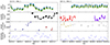 |
Fig. 1. Light curves of NuSTAR, NICER, and IBIS/ISGRI during IXPE Obs. 1 (left panel) and Obs. 2. (right panel). In the top row of each panel the three IXPE DU light curves are shown (DU1 blue, DU2 orange, and DU3 green). In the left panel the NICER soft purple and dark red points correspond to ObsID 6010230101 and 6010230102. In the right panel the NuSTAR red and purple points correspond to ObsIDs 90902310004 and 90902310006. The NICER gray points correspond to ObsID 6010230106. |
List of observations.
The normalized Stokes parameters q = Q/I and u = U/I, the PD, and polarization angle (PA) with their uncertainties can be calculated by using the model-independent pcube binning algorithm of IXPEOBSSIM. On the other hand, PD and PA obtained with XSPEC require the definition of a spectropolarimetric model. Because the PD and PA are not independent, the appropriate way to report the results is by means of contour plots at certain confidence levels for the joint measurements of the two parameters. We report the XSPEC (PD, PA) contour plots obtained by using the steppar command, while the contour plots associated with the IXPEOBSSIM analysis were obtained from the statistics of the number of counts (Weisskopf et al. 2010; Strohmayer & Kallman 2013; Muleri 2022).
The spectropolarimetric analysis was carried out by taking into account the current IXPE effective area instrument response function (arf), which may not be as accurate as possible at energies above 6 keV where there is a significant roll-off in the spectral response. Because the high-energy part of the IXPE band is of special interest for our study, we estimate the IXPE spectral systematic uncertainties to be 3% in Obs. 1 and 2% in Obs. 2, based on the comparison with the NICER, NuSTAR, and IBIS/ISGRI energy spectra. The spectral models for both the IXPE observations are frozen based on the spectral analysis of these other observatories. We used the XSPEC gain fit tool for the IXPE data only, to shift the energies on which the response matrix is defined and to match the effective area curve during the fit procedure. The spectropolarimetric fit of the IXPE data was carried out freeing the three DU normalization constants: the gain slope, the gain offset, and the polarimetric parameters3.
2.2. NuSTAR
GX 5−1 was observed by NuSTAR (Harrison et al. 2013) on March 21 and twice on April 13–14, 2023. All the relevant observation times, sequence IDs, and exposure times are provided in Table 1, and the corresponding light curves are shown in Fig. 1. The unfiltered event files were processed with the NuSTAR Data Analysis Software (NUSTARDAS v.2.1.2) to produce the cleaned and calibrated level 2 data using the latest calibration files (CALDB v.20221130) and the standard filtering criteria with the nupipeline task, where statusexpr"STATUS==b0000xxx00xxxx000" was set, due to the source flux exceeding 100 counts s−1. The spectra and light curves were extracted using the nuproducts task, selecting a circular region of 60″ in radius centered on the source.
2.3. NICER
NICER (Gendreau et al. 2016) observed GX 5−1 between March 21–25 and April 13–14, 2023. The observations identified with IDs 6010230101, 6010230102, and 6010230106 were included in the spectropolarimetric analysis because they are simultaneous with the IXPE observations. The calibrated and cleaned files were extracted by using the standard nicerl2 command of the NICER Data Analysis Software (NICERDAS v.10) together with the latest calibration files (CALDB v.20221001). The spectra and the light curves were then obtained with the nicerl3-spect and nicerl3-lc tasks, while the background was computed using the SCORPEON4 model. The light curves were obtained including 50 NICER FPMs available during the ObsIDs included in the analysis (out of 52 available, excluding noisy detectors ID 14 and ID 34). Thus, no discontinuities in the NICER light curves are present (see Fig. 1).
During the contemporary observation with IXPE there were two significant increases in count rate in the NICER data, up to twice the typical value. These events were coincident with two solar flares; the first was a C-class flare peaking at about 60048.5389 MJD and the second was an M-class flare peaking at about MJD 60048.6806. We removed them manually from the GTIs (the C-class flare from MJD 60048.53535 to MJD 60048.60033 and the M-class flare from MJD 60048.67506 to MJD 60048.73744).
We found some relevant features in the energy spectrum below 4 keV, most likely due to spectral features unaccounted for in the NICER ARF. Because of the source’s high count rate, these features become apparent in the spectral modeling. We therefore accounted for calibration artifacts owing to imperfections in modeling the dead layer of the silicon detector at the Si-K edge, and of the concentrator mirror surface roughness at the Au-M edges, which affects the ≈2.2–3.5 keV range5. We froze the energy of the edges at their best-fit value, as reported in Table 4.
2.4. INTEGRAL IBIS/ISGRI
INTEGRAL IBIS/ISGRI (Winkler et al. 2003) observed the region of GX 5−1 from March 21 to 22 and from April 13 to 15, 2023, responding to a request by the IXPE team. The data for this source are publicly available and were reduced for the imager IBIS (Ubertini et al. 2003) and the ISGRI detector (Lebrun et al. 2003). We used the MMODA6 platform that empowers the Off-Line Science Analysis (OSA) version 11.2 distributed by the ISDC (Courvoisier et al. 2003) with the most recent calibration files that are continuously pushed in the instrument characteristic repository. We first built a mosaicked image of all individual pointings that constitute the standard dithering strategy of observation for IBIS/ISGRI in the 28–40 keV energy range. These images were used to make the catalog of detected sources with a signal-to-noise ratio higher than 7. Using these catalogs, we extracted light curves with 1000 s time bins and spectra in 256 standard channels for IBIS/ISGRI, these were grouped in ten equally spaced logarithmic channels between 28 and 150 keV. We also accounted for a systematic uncertainty of the spectra at the 1.5% level. The equivalent on-axis exposures of the IBIS/ISGRI spectra are 40 and 85 ks, respectively, after correction for dead time and vignetting. The products are available at the INTEGRAL Product gallery7.
2.5. ATCA
The Australia Telescope Compact Array (ATCA) observed GX 5−1 on March 24 and April 14, 2023. On March 24, the telescope observed with the array in its 750C configuration8. Observations taken on April 14 were carried out with the array in a relatively compact H214 configuration, in combination with an isolated antenna located 6 km from the array core, which was also included in our analysis. For both observations the data were recorded simultaneously at central frequencies of 5.5 GHz and 9.0 GHz, with 2 GHz of bandwidth at each frequency.
We used PKS 1934−638 for bandpass and flux density calibration. PKS 1934−638 was also used to solve for the antenna leakages (D-terms) for the polarization calibration. The nearby source B1817−254 was used for gain calibration and to calibrate the PA using the Common Astronomy Software Applications for radio astronomy (CASA, version 5.1.2; CASA Team 2022) atcapolhelpers.py task qufromgain9. Calibration and imaging followed standard procedures within CASA. When imaging, we used a Briggs robust parameter of 0 to balance sensitivity and resolution (Briggs 1995), and to suppress the effects from some bright diffuse emission within the field.
For our March 24 observations, fitting for a point source in the image plane, we detected GX 5−1 at a flux density of 960 ± 19 μJy at 5.5 GHz and 810 ± 11 μJy at 9 GHz coincident with the previously reported radio position (e.g., Berendsen et al. 2000; Liu et al. 2007). These detections correspond to a radio energy spectral index of −0.37 ± 0.09. The Stokes Q and U values were measured at the position of the peak source flux density (Stokes I). No significant linearly polarized (LP) emission was detected at either frequency. Measuring the root mean square of the image noise in a 50″ × 50″ region over the source position (taken as 1σ), provides 3σ upper limits on the polarized intensity  of 58 μJy beam−1 at 5.5 GHz and 48 μJy beam−1 at 9 GHz. These correspond to a 3σ upper limit on the PD of 6.1% at 5.5 GHz and 5.9% at 9 GHz. Stacking the two frequencies to maximize the sensitivity also yields a nondetection of linearly polarized emission, with a 3σ upper limit of 4.2% (centered at 7.25 GHz).
On April 14, following the same calibration and imaging procedure, we measured the flux density of GX 5−1 to be 750 ± 50 μJy and 620 ± 40 μJy at 5.5 and 9 GHz, respectively. These detections correspond to a radio spectral index of −0.4 ± 0.1. We note that due to the more compact array configuration for this epoch, and the presence of diffuse emission in the field, we imaged with a strictly uniform weighting scheme (setting the Briggs robust parameter to −2), reducing the impact of diffuse emission in the field on our resultant images. The compact configuration coupled with a shorter exposure time resulted in a higher noise level in the images. At 5.5 GHz, we do not detect any linearly polarized emission, with a 3σ upper limit on the PD of 12.5%. Similarly, at 9 GHz we measure a 3σ upper limit on the PD of 20%. Stacking the two frequencies places a 3σ upper limit on the PD of 8% at 7.25 GHz. We note that during the final ∼30 min of the observation, some linear polarization was detected close to the source position, but only at 9 GHz. Due to the nondetection at 5.5 GHz and the short and sudden nature of this emission, we attribute it to radio frequency interference and not an astrophysical event.
2.6. VLT VISIR
Mid-IR observations of the field of GX 5−1 were made with the European Southern Observatory’s Very Large Telescope (VLT) on March 28 and 31, 2023, under program 110.2448 (PI: D. Russell). The VLT Imager and Spectrometer for the mid-Infrared (VISIR; Lagage et al. 2004) instrument on the VLT was used in small-field imaging mode. Four filters (M-band, J8.9, B10.7, and B11.7) were used, with central wavelengths of 4.67, 8.70, 10.64, and 11.51 μm, respectively. For each observation, the integration time on source was composed of a number of nodding cycles, chopping and nodding between source and sky. The total observing time was usually almost twice the integration time.
Observations of standard stars were made on the same nights as the target, in the same filters (photometric standards HD 137744, HD 169916, HD 130157, and HD 145897 were observed, all at airmass 1.0–1.1). Conditions were clear on both nights. All data (target and standard stars) were reduced using the VISIR pipeline in the GASGANO environment10. Raw images from the chop–nod cycle were recombined. Photometry was performed on the combined images using PHOT in IRAF11. For the B10.7 filter, two standard stars were observed on each night, just before and after each observation of GX 5−1, to check for stability. We found that the counts-to-flux ratio values from these standards agree to a level of 6.4%, which we adopt as the systematic error of all flux measurements. The estimated counts-to-flux ratio in each filter was used to convert count rates (or upper limits) of GX 5−1 to flux densities.
On March 28, 2023 (MJD 60031.37), the B10.7 filter was used only, and we derive a 3σ flux density upper limit of 3.27 mJy at 10.64 μm (the airmass was 1.05–1.10). On March 31, 2023 (MJD 60034.34), GX 5−1 was detected in M-band and J8.9, with flux densities of 4.2 ± 1.4 mJy at 4.67 μm and 10.0 ± 2.3 mJy at 8.70 μm, respectively (at airmass 1.07–1.17). The significance of the detection was 5.9σ in both filters. The errors on the fluxes incorporate the statistical error on each detection, and the systematic error from the standard stars, in quadrature. The source was not detected in the B10.7 and B11.7 filters on March 31, 2023, with flux upper limits that were less constraining than on March 28, 2023.
GX 5−1 lies in a crowded region of the Galactic plane, with several stars detected within 5″ of the source. The near-IR counterpart was confirmed through photometry and spectroscopy (named star 513; Jonker et al. 2000; Bandyopadhyay et al. 2003), and its coordinates agree with the radio and X-ray position. We are confident that the source we detect with VISIR is indeed GX 5−1 because star 503 from Jonker et al. (2000) and Bandyopadhyay et al. (2003) is also detected (at a low significance of 3.1–3.3σ) at the correct coordinates. This star is estimated from Fig. 1 of Jonker et al. (2000) to lie 4 3 to the southeast of GX 5−1. In the J8.9 VISIR image the detected source is measured to be 4
 28 to the southeast of the position of the detected GX 5−1, as expected. The flux density of star 503 is 1.4 ± 0.5 mJy in M-band and 4.5 ± 2.2 mJy in J8.9.
2.7. REM and LCO
Optical (SDSS griz filters) and near-infrared (NIR; 2MASS H-band) observations of GX 5−1 were acquired with the robotic 60 cm Rapid Eye Mount (REM; Zerbi et al. 2001; Covino et al. 2004) telescope on March 22 and on April 14, 2023 (see Table 1). Strictly simultaneous observations were obtained in all bands; on March 22, a series of 150 exposures of 30 s each were acquired in H-band (dithering was applied), and 20 exposures of 300 s in each of the optical bands; on April 14, a series of 225 exposures of 30 s were acquired in H-band (dithering was applied), and 30 exposures of 300 s in each of the optical bands.
Optical observations were also acquired with the 1 m and 2 m telescopes of the Las Cumbres Observatory (LCO) network, using the i′ and Y filters. Observations with the 2 m telescope (Siding Spring – Faulkes Telescope South) were performed on 2023-03-22T16:33:07; 2023-03-29T15:50:11; 2023-03-30T15:46:39; and 2023-03-31T15:43:07 (300 s integration in all epochs and bands), and with the 1 m telescopes (at the locations of Cerro Tololo, Siding Spring, and Sutherland) on 2023-03-21T07:09:39; 2023-03-22T01:01:36; 2023-03-22T08:11:35, and 2023-04-14T05:35:19, T08:11:37, T15:11:30, and T23:23:55 (300 s integration in all epochs and bands).
The optical images were bias- and flat-field corrected using standard procedures; the contribution of the sky in the NIR images was evaluated by performing a median of the dithered images five-by-five, and was then subtracted from each image. In all bands and epochs, all the reduced images were then aligned and averaged in order to increase the signal-to-noise ratio. Aperture photometry was performed using PHOT in IRAF. Flux-calibration was performed against a group of six stars with magnitudes tabulated in the 2MASS catalog12 and six stars from the PanSTARRS catalog13.
Due to the very high extinction of the source (NH = 4.93 × 1022 cm−2 and 4.88 × 1022 cm−2, which translates14 into AV = 17.2 mag and 17 mag in Obs. 1 and Obs. 2, respectively) and to the combination of the low spatial resolution of our images and the crowded field of the source, GX 5−1 is not detected in any of the optical and NIR images acquired. A blend of our target with at least one of the nearby stars can be detected at very low significance in the averaged H-band image, at a position consistent with the proposed optical and NIR counterpart of the source (Jonker et al. 2000, star 513). However, this detection is not significant enough to extract a flux for the blend.
We estimate the following 3σ upper limits (only the most constraining ones per epoch are quoted): H = 13.84, Y = 19.08, z = 18.28, i′ = 21.79 (LCO), r′ = 20.22, g′ = 20.45 for Obs 1; H = 14.00, Y = 18.86, z = 18.35, i′ = 21.22, r = 20.46, g = 20.50 for Obs 2. These upper limits are consistent with the H-band magnitude of the proposed NIR counterpart reported by Jonker et al. (2000) (Star 513; H = 14.1 ± 0.2).
3. Results
3.1. Polarimetric model-independent analysis
The model-independent analysis of the X-ray polarization with ixpeobssim (see Table 2) in the 2–8 keV energy band gives the PD of 4.3%±0.3% and 2.0%±0.3% in Obs. 1 and Obs. 2, respectively (with 1σ errors). The corresponding PAs are  and
and  . We see a significantly larger PD in Obs. 1 compared to Obs. 2. However, the PA is compatible with being constant during the two observations. The contour plots of the IXPEOBSSIM analysis in the 2–8 keV energy range are reported in Fig. 2 (dashed lines).
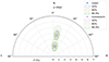 |
Fig. 2. Polarization of GX 5−1 measured by IXPE in the 2–8 keV energy range during Obs. 1 and Obs. 2 obtained with XSPEC and IXPEOBSSIM. The contours are computed for the two parameters of interest at 50%, 90%, and 99.9% confidence levels. |
The behavior of polarization as a function of energy is reported in Table 2. The energy dependence of the PD is essentially the same in the two observation, whereas the PA varies from positive to negative values. A proper assessment of this behavior requires the use of Stokes parameters. The left panels of Fig. 3 show the Stokes parameters as a function of energy of the two observations separately. For each observation, the Stokes q parameters are consistent with being constant in energy, albeit at different values between the first and second observations. On the other hand, the Stokes u parameters are not compatible with a constant (see Obs. 1 and Obs. 2 columns of Table 3). This requires the variation in PA.
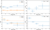 |
Fig. 3. Stokes parameters as a function of energy for IXPE Obs. 1 and Obs. 2 (left panels) and for the combined data set (right panels) obtained with IXPEOBSSIM. The normalized Stokes q parameter is compatible with a constant value in each of the IXPE observations, whereas the Stokes u parameter is not (see Table 3). This behavior of the Stokes parameters is consistent with a variation in PA (see Fig. 4). |
Results of the Stokes parameters fit with a constant value for Obs. 1, Obs. 2, and the combined data set.
On the basis of the assumption that the geometry and the physical process producing polarization are the same in the two observations, we also calculated the Stokes parameters of the IXPE observations combined (Obs. 1 and Obs. 2) to improve the statistics. While the resulting normalized Stokes parameter q remains compatible with a constant value, the Stokes u is even farther from being a constant with the reduced χ2 values for ν = 3 degrees of freedom being  = 1.26 and
  = 7.16 for q and u, respectively. As anticipated by the separate analysis of the two observations, this behavior of q and u implies a variation in PA. Such a variation of about 20° is highlighted in Fig. 4. In the top panel the contour plots on the PD–PA plane for the IXPE whole observation are shown. Polarization in the 2–3 keV energy bin is not compatible with that in the 5–8 keV bin with a probability of ∼98.7%. In the bottom panel the variation in PA with energy is shown together with the fit by a constant giving a value of
  with
with  = 6.44 for ν = 3 corresponding to a significance level α = 0.02%.
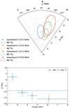 |
Fig. 4. Polarization contour plot (top panel) and PA (bottom panel) as a function of energy of the combined IXPE data set (Obs. 1 and Obs. 2). |
3.2. X-ray spectral analysis
The NICER, NuSTAR, and IBIS/ISGRI light curves contemporary to IXPE observations are shown in Fig. 1. The time-resolved CCD and hardness-intensity diagram (HID) for all the observations with IXPE, NICER, and NuSTAR show GX 5−1 moving along the complete Z-track from March 21 to April 14. NuSTAR CCD and HID, obtained from the GTIs contemporary to the IXPE observations (see Fig. 5), highlight clearly the Z shape, disentangling also the NB with respect to the FB, due to the wide energy band from 3 to 20 keV used to construct the CCD colors. During IXPE Obs. 1 the source was in the HB, whereas it was in the NB-FB during Obs. 2, which we checked by constructing the CCD and HID from the IXPE data of the two observations. From March 24 to 25 (about 3 days after the end of Obs. 1), when ATCA was observing, NICER detected GX 5−1 moving from the HB-NB corner toward the NB.
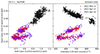 |
Fig. 5. NuSTAR CCD and HID of GX 5−1 contemporary to IXPE observation. During IXPE Obs. 1 the source was in the HB, while during Obs. 2 it was in the NB-FB. The observing days March 21, April 13, and April 14, 2023, are shown in black, red, and purple, respectively. |
We fit the NICER, NuSTAR, and IBIS/ISGRI data of Obs. 1 and Obs. 2 and present the results in Fig. 6 (where the IXPE energy spectrum is overplotted to the frozen model) and Table 4. The better fits we obtained are based on the following spectral models for Obs. 1 and Obs. 2:
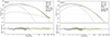 |
Fig. 6. Deconvolved energy spectrum of GX 5−1. The top panels show the deconvolved NICER (1.5–10 keV), NuSTAR (3.5–45 keV for Obs. 1 and 3.5–35 keV for Obs. 2), and IBIS/ISGRI (28–50 keV) spectra simultaneous with both IXPE observations, obtained from the best-fit model in Table 4. The IXPE (2–8 keV) energy spectrum is overplotted on the frozen model. The bottom panels show the residuals between data and model in units of σ. |
Best-fit parameters of GX 5−1 spectral model from NICER, NuSTAR, and IBIS/ISGRI data simultaneous to IXPE observation.
tbabs*(diskbb+expabs*powerlaw+thcomp*bbodyrad),
tbabs*(diskbb+thcomp*bbodyrad),
respectively.
We included the normalizing cross-calibration multiplicative factors for the NICER, IBIS/ISGRI, and NuSTAR FPMA (frozen at unity) and FPMB telescopes. A tbabs (Wilms et al. 2000) multiplicative model component was used to take into account the low-energy absorption due to the interstellar medium. We used the abundances and cross-section tables according to Wilms et al. (2000) and Verner et al. (1996) (wilm, vern in XSPEC). We modeled the GX 5−1 energy spectra of both the observations with a multicolor disk and a harder boundary layer (BL) or spreading layer (SL) emission (e.g., Popham & Sunyaev 2001; Revnivtsev et al. 2013). In both observations, the convolution model component thcomp (Zdziarski et al. 2020) is used to represent Comptonized emission from the BL–SL (e.g., Di Salvo et al. 2002; Farinelli et al. 2009) modeled with the bbodyrad component. The f parameter of thcomp represents the fraction of Comptonized seed photons. In Obs. 1 this parameter is > 0.63 with the best-fit value equal to 0.99. Effectively, all photons from the BL–SL bbodyrad are Comptonized. In Obs. 2 only a fraction between 2.7% and 11.2% (best-fit 3.2%) of seed photons are Comptonized. It is worth noting that a higher Comptonization fraction corresponds to a higher PD observed from the source. During Obs. 1, when the source is on the HB, the energy spectrum is harder, and a high-energy excess was seen (but absent in Obs. 2). This excess is modeled with an additional hard tail represented by a power-law component with a low-energy exponential roll-off. The e-folding energy for the absorption of the exponential roll-off is set equal to the bbodyradkTbb energy of the SL–BL. This parameter link comes from the assumption that the power-law emission originates from the seed distribution of the SL–BL blackbody. The BL and the inner disk are hotter in Obs. 2 than in Obs. 1, while the BL sphere-equivalent radius and inner disk radius are larger in Obs. 1. In contrast to Obs. 1, the additional power-law component is not needed to model the spectrum of Obs. 2.
The softer disk component dominates up to ∼3.5 keV in Obs. 1 and up to ∼5.5 keV in Obs. 2 (see Fig. 6). In the 2–8 keV band, the energy flux in the Comptonized component (including the contribution of the exponentially absorbed power-law component) accounts for ∼61% of the total in Obs. 1. In Obs. 2 the energy flux of the Comptonized component drops to ∼33% of the total in the same energy band.
3.3. X-ray spectropolarimetric analysis
The results of the spectropolarimetric analysis, including IXPE, once the spectral model used to fit the data from the other observatories is frozen, is reported in Table 5. The PD obtained with a polconst multiplicative model component applied to the whole spectral model of GX 5−1 in Obs. 1 and Obs. 2 is 3.7%±0.4% and 1.8%±0.4%, respectively. The PA is around −9° in both the observations. The polarization contour plot in the 2–8 keV energy band obtained with XSPEC (polconst model applied to the spectral model) is shown in Fig. 2. These contours are nearly identical to those obtained using IXPEOBSSIM.
Best-fit parameters of polarization analysis with XSPEC.
The spectropolarimetric analysis with XSPEC allows us to assign a polarization to the different spectral components. The result of this analysis is reported in Table 5 and Fig. 7. For Obs. 1 we assigned the same polarization for the expabs*powerlaw and thcomp*bbodyrad components, assuming that the power law is just a continuation of the BL–SL component, with the power-law low-energy rollover Ecut being equal to the temperature of the BL–SL bbodyradkTbb.
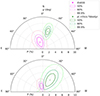 |
Fig. 7. Polarization contour plots from the spectropolarimetric analysis in the 2–8 keV energy range of Obs. 1 (top panel) and Obs. 2 (bottom panel). The polconst polarimetric model is applied separately to the diskbb component of both IXPE observations and to the (expabs*powerlaw+thcomp*bbodyrad) components as a whole. The expabs*powerlaw component (labeled pl. in the legend) is included only in Obs. 1. Contour plots are computed for the four parameters of interest, taking into account the fact that the polarization of the disk and Comptonization components are correlated in the simultaneous fit. |
The Comptonization component is well constrained at a 99.9% confidence level only in Obs. 1, while the disk component is not constrained at 99% in either observation (see Fig. 7). Moreover, in both the observations the polarization of each component has similar PAs, suggesting that the geometry responsible for the polarization is similar. Figure 8 shows the fit of the Q and U Stokes parameters as a function of energy with the two polconst components for both the observations. The contribution to the total flux of the polarized component is different (higher in Obs. 1) probably due to a dilution effect by unpolarized radiation connected with a low covering fraction of the Comptonization component (see Table 4). Unfortunately, even if the source was active in the radio band during the observation campaign, it is impossible to compare the direction of the PA with the direction of the jet because the radio observations reported in this paper do not have the spatial resolution to resolve it. Moreover, the literature does not report any information about jet direction.
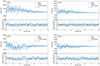 |
Fig. 8. Fit of the IXPE Stokes parameters Q and U as a function of energy with the model comprising two polconst components applied to the disk (dotted lines) and to the Comptonization (dashed lines) for Obs. 1 (left column) and Obs. 2 (right column). |
The variation in PA of the total emission, reported in Sect. 3.1, obtained with the IXPEOBSSIM model independent analysis can be explained by the different PAs of the disk and the Comptonized spectral components that are neither aligned nor 90° apart. The PA of the total emission varies from being positive at lower energies (dominated by the diskbb component) to negative values at higher energies dominated by the Comptonization component with a positive PA.
When assessing polarization as a function of time, no significant variations are seen. This implies that polarization is not sensitive to the flux variation present in the light curves (see Fig. 1).
3.4. Spectral energy distribution
Thanks to the multi-energy observation campaign it was possible to produce a broadband (radio–X-ray) spectral energy distribution (SED) of GX 5−1 for both the observations (see Fig. 9). Optical and infrared fluxes were de-reddened using the hydrogen column density reported in this work (NH = 4.93 × 1022 cm−2 and 4.88 × 1022 cm−2 in Obs. 1 and 2, respectively), which was converted into an estimate of the V-band extinction AV using the relation reported in Foight et al. (2016), resulting in AV = 17.18 ± 0.77 mag and 17.00 ± 0.72 mag for the two observations, respectively. The different absorption coefficients at optical and near-IR wavelengths were then evaluated using the relations reported in Cardelli et al. (1989) and Nishiyama et al. (2008), respectively. For the mid-IR, the coefficients reported in Weingartner & Draine (2001) were used instead.
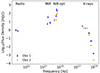 |
Fig. 9. Broadband radio to X-ray SED of GX 5−1 during the two observations. For Obs. 2 no mid-IR flux is reported as observations were not performed with VISIR at that time (see Sect. 2.6 for details). The flux densities at mid-IR, near-IR, and optical frequencies have been de-reddened (as described in Sect. 3.4). The errors are at 68% confidence level. |
GX 5−1 is detected at radio and mid-IR wavelengths, with upper limits in the near-IR and optical. As mentioned in Sect. 2.7, this is due to the high value of dust extinction of AV ≈ 17. This implies an extinction of ∼7 mag at 1 μm (Y-band) and ∼3 mag at 1.6 μm (H-band). The radio spectral index of −0.4 ± 0.1 is too steep for the radio emission to arise from a steady compact jet (for which we expect a spectral index from ∼0 to +0.5). As such, it is likely due to optically thin jet ejections or to a combination of compact jet and optically thin ejections. In the mid-IR we report the first detection of this source. The de-reddened flux densities are comparable to the near-IR values reported in the literature (Naylor et al. 1991; Jonker et al. 2000; Bandyopadhyay et al. 2003); however, the de-reddened near-IR fluxes depend sensitively on the value of the interstellar extinction. We note that different values of the neutral hydrogen column densities are reported in the literature, ranging from NH = 2.54 × 1022 cm−2 to 6.20 × 1022 cm−2 (Christian & Swank 1997; Zeegers et al. 2017; Homan et al. 2018; Clark 2018; Bhulla et al. 2019). Yang et al. (2022) has derived NH = (4.52 ± 0.01)×1022 cm−2 by measuring the Si K edge due to scattering by dust using the Chandra gratings. This value is in agreement with our measurements because NH is slightly overestimated when fitting the continuum with the absorption model tbabs (Corrales et al. 2016). In this work we observed GX 5−1 over a significantly larger energy range, and we are confident to have properly constrained the absorption in the interstellar medium. However, if there is a component of the neutral hydrogen column that is intrinsic to the LMXB, this could cause varying measurements and introduce uncertainty into the relation between NH and the extinction AV. Moreover, older works using Anders & Grevesse (1989) solar abundances rather than Wilms et al. (2000) interstellar abundances, could be affected by model systematics.
The mid-IR flux measured with the VLT VISIR is higher than the extrapolation of the ATCA spectral index from radio to mid-IR. The mid-IR emission is therefore unlikely to be due to optically thin synchrotron emission from discrete jet ejections that were seen in the radio, but it could be optically thin synchrotron emission from the compact jet (from above the jet spectral break; Russell et al. 2013). We find evidence of strong mid-IR variability between the two epochs, with the 9–11 μm flux density changing from < 3.27 mJy on March 28, 2023, to 9.95 ± 2.31 mJy on March 31, 2023. While this variation by a factor of ≥3 (≥2.5 magnitudes) is quite high for a LMXB accretion disk on these timescales, high amplitude (spanning several magnitudes) infrared variability has been reported from a number of bright persistent NS-LMXBs, including GX 17+2, Cir X-1, 4U 1705−440, and GX 13+1 (e.g., Glass 1994; Callanan et al. 2002; Bandyopadhyay et al. 2002; Homan et al. 2009; Corbet et al. 2010; Harrison et al. 2011). This variability has generally been interpreted as indicative of highly variable synchrotron emission from a compact jet. Variable near-IR polarization has also been reported from the bright persistent NS-LMXBs Sco X-1 and Cyg X-2, and from the NS-LMXB transient SAX J1808.4−3658 (Shahbaz et al. 2008; Russell & Fender 2008; Baglio et al. 2020). The de-reddened mid-IR 4.7–8.7 μm spectral index on March 03, 2023, is −2.3 to −0.4 (adopting AV = 17.18 ± 0.77), which is consistent with optically thin synchrotron emission from relativistic particles or with a steeper particle distribution with a thermal (Maxwellian) component, as has been seen at infrared wavelengths from jets in some black hole LMXBs (e.g., Russell et al. 2010; Shahbaz et al. 2013). Thus, this emission could originate from a compact jet that peaks in the mid- or far-IR, although follow-up observations characterizing the IR spectrum and variability would be beneficial to confirm the nature of the IR emission. If the compact jet is present, its spectrum from radio to mid-IR must be inverted, with index > 0.33 (and fainter than the observed radio emission). The radio to IR spectrum is similar in some ways to the NS-LMXBs 4U 1728−34 and 4U 0614+091 (Migliari et al. 2010; Díaz Trigo et al. 2017).
3.5. Measurement of the distance to the source
In order to derive some spectral model parameters (namely  of diskbb and Rbb of bbodyrad), an estimate of the distance to the source is needed. This estimate can be obtained from the equivalent hydrogen column density NH, which we obtain from our analysis. We find that
  cm−2 and
  cm−2 for the first and the second observations, respectively. Because the two values are the same at the 90% confidence levels, we use the average value and its largest uncertainty range,
  cm−2, in the following discussion. To estimate the distance to the source we adopt the approach proposed by Gambino et al. (2016). We use the model of the infrared Galactic interstellar extinction discussed by Marshall et al. (2006). Because the Galactic coordinates of GX 5−1 are
  and
and  , we adopt the map that relates the infrared extinction AKs with the source distance d valid for l = 5° and b = −1° (see black dots with the error bars in Fig. 10).
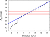 |
Fig. 10. Fit of the infrared extinction AKs between 5 and 15 kpc from Marshall et al. (2006) with a linear function (the best-fit line and the lines taking into account the associated errors are in blue). The red horizontal lines represent the estimate with the corresponding upper and lower limits of AKs from Eq. (3). The distance to the source is thus d = 7.6 ± 1.1 kpc. |
Because the visual extinction AV is related to NH as (Foight et al. 2016)
 (1)
(1)
and the relation between AV and the extinction in the Ks band is (Nishiyama et al. 2008)
 (2)
(2)
we obtain
 (3)
(3)
We fit the AKs values between 5 and 15 kpc with a linear function (the best-fit line and the lines taking into account the associated errors are in blue in Fig. 10). We infer that the distance to the source is d = 7.6 ± 1.1 kpc. This distance is in agreement with the previously reported values (Penninx 1989; Smith et al. 2006).
4. Discussion
As shown in Sect. 3, the two multiwavelength observations of GX 5−1 allowed us to catch the source when it was covering the complete Z-track on its CCD–HID (see Fig. 5). In particular, during the first observation GX 5−1 was on the HB of the track, while in the second observation it moved across to the NB and FB. Very interestingly, we found the same behavior in the peculiar transient XTE J1701−462 (Cocchi et al. 2023), where the PD was correlated with the source position on the Z-track, being higher in the HB and decreasing by a factor of about two in the NB. Long et al. (2022) hypothesized the same behavior also for Sco X-1. There are at least three regions that may potentially contribute to the polarization: the BL–SL, the accretion disk, and the reflection of the BL–SL photons from the disk atmosphere or a wind.
The spectropolarimetric analysis of the IXPE data (Table 5) shows that the disk polarization is about 2% in both observations, which is compatible with the classical results of a high optical depth scattering atmosphere at an inclination of 60° (Chandrasekhar 1960). The higher PD value of the hard component, on the other hand, cannot be explained by repeated Compton scattering in high optical depth environments, neither for a boundary layer coplanar with the disk (which otherwise would resemble a Chandrasekhar-like slab) nor for a spreading layer around the neutron star, for which a maximum PD of ≲2% is expected.
Disk reflection is probably the most natural way to explain a PD on the order of 4%–5%, as shown by Lapidus & Sunyaev (1985). It is important to note that we do not find a strong reflection signature in the spectral analysis, and it deserves mentioning that the reflection contribution to the spectrum may be low, and sometimes may be embedded in the continuum, but can nevertheless make a large contribution to the net polarization signal (Schnittman & Krolik 2009). This may be particularly true if the primary spectrum is not a hard power law, but a blackbody-like spectrum with a rollover below 30 keV. We note that a similar argument has been used also for Cyg X-2 (Farinelli et al. 2023) and GX 9+9 (Ursini et al. 2023) to explain the high PD attributed to the Comptonization spectrum in a twofold spectropolarimetric approach.
The PD of the reflected radiation is not easy to predict because it depends on geometrical and physical factors (e.g., the disk ionization parameter); however, it is not likely to exceed ∼20% (Matt 1993; Poutanen et al. 1996; Schnittman & Krolik 2009). We tested the hypothesis of whether there is a reflection component in the GX 5−1 energy spectrum by making some assumptions: (1) a highly ionized disk due to the absence of a broad emission line in the Fe-K region of the spectrum; (2) inclination i = 60° since GX 5−1 is a Cyg-like Z-source (Homan et al. 2018; 3) the reflection amplitude f = Ω/2π kept at a typical value for the NS-LMXBs (namely 30%; see, e.g., Di Salvo et al. 2015; Matranga et al. 2017). We applied the following spectral models:
The comptb model (Farinelli et al. 2008) component was included in place of the thcomp to prevent a double convolution of the BL–SL blackbody. Details on rfxconv and rdblur model components can be found in Kolehmainen et al. (2011) and Fabian et al. (1989), respectively. The sum rdblur*rfxconv*comptb + comptb accounts for the reflected radiation (the first term) plus the incident radiation (the second term).
This modeling of the reflection component contribute ∼22% of the flux in Obs. 1 and ∼12% in Obs. 2. This contribution to the total emission can easily account for the polarization detected (see Table 6 for details of the fit parameters of the energy spectrum). The fraction of Comptonized photons in Obs. 2 is significantly smaller with respect to Obs. 1, as also obtained in Sect. 3 by applying only the Comptonization model thcomp. The parameter  in comptb corresponds to a
  of photons upscattered in energy (consistent with
  obtained when reflection is not taken into account as in Sect. 3). This confirms the presence of a blackbody component observed through an almost vanished Comptonization medium in Obs. 2, even if reflection is included. However, the fraction of Comptonized photons, albeit small (∼3%), is still sufficient to manifest its presence at high energy. If we were to neglect this small fraction of Comptonized photons by substituting comptb with a blackbody component, such as bbodyrad, we would obtain an unacceptable fit result (
 = 3.6, with a significant excess at high energy due to this small fraction of Comptonized photons).
Best-fit parameters with reflection included in the energy spectrum model of GX 5−1 from NICER, NuSTAR, and INTEGRAL data simultaneous to IXPE observations.
Another possible mechanism for producing polarization is related to scattering in the wind above the accretion disk. As was shown in Sunyaev & Titarchuk (1985), the emission scattered once in a plane (e.g., equatorial wind) can be polarized up to 27% for an inclination i = 60°. This polarization degree is only weakly dependent on the opening angle of the wind. Assuming that 20% of the source emission is scattered, we can obtain the observed PD. Recently, a similar model was shown to explain well the presence of a constant polarized component in the X-ray pulsars RX J0440.9+4431/LS V +44 17 (Doroshenko et al. 2023). Although it is well known that strong winds can indeed be present in the soft states of X-ray binaries (e.g., Neilsen & Lee 2009; Ponti et al. 2012, 2014), it is worth noting that we do not see wind absorption features in the energy spectrum of GX 5−1, implying that, if present, the wind should be completely ionized.
Both IXPE observations show similar behavior of the PD values: they are smaller in the 2–4 keV band and increase slightly with energy. The reduction of the PD at lower energies can be explained by the energy dependence of the disk emission. In the low-energy band we have a marginally polarized disk emission dominating the spectrum, while at higher energies the emission of the SL and/or the scattered or reflected component is more visible. Another feature of the observed emission that needs to be addressed is the variation in PA with energy. In the spectropolarimetric analysis the disk and the Comptonization components have nonorthogonal PAs, and thus the variation in polarization plane of the total emission with energy can be interpreted as the energy-dependent contribution of these two components to the total emission. The same applies if, for instance, the SL emission is scattered in the wind and the disk emission is polarized with a different and nonorthogonal angle. The PA of the combined emission will be energy dependent. It is well known that the disk emission exhibits a rotation of the polarization plane with energy (Connors et al. 1980; Dovčiak et al. 2008; Loktev et al. 2022). Simulations of the SL emission also show a change in PA with energy, but predict a PD at most of 1.5% (Bobrikova A., in prep.). Thus, a single component explanation of the PA variation cannot be considered compatible with the high measured PD. Further modeling will be needed to satisfactorily address the explanations presented above.
5. Summary
IXPE observed the NS-LMXB GX 5−1 twice in the period March–April 2023. Contemporary observations in the X-ray energy band were put in place with NICER, NuSTAR, and INTEGRAL. Multiwavelength coverage was ensured by ATCA in the radio, VLT VISIR in mid-IR, REM in optical, and NIR and LCO in the optical.
During the observations GX 5−1 moved across the entire Z-track. NuSTAR clearly disentangled the NB with respect to the FB, thanks to its extended energy band. The presence of a hard tail, reported in previous analyses, was clearly detected in Obs. 1, but not in Obs. 2, when the source had a softer energy spectrum. The X-ray PD was ∼4% during Obs. 1 when the source was in the HB and ∼2% during Obs. 2 with the source in the NB-FB. This result is in agreement with findings from the other Z-sources observed by IXPE (namely Cyg X-2 and XTE J1701−462).
The source manifested an unexpected variation in PA as a function of energy, by ∼20°. The magnitude of the variation combined with the magnitude of the PD require further modeling. However, it is likely related to the different PAs of the disk and Comptonization components, which are nonorthogonal and, moreover, have emission peaks at different energies.
In the radio band the source was detected, but only upper limits to the polarization were obtained (∼6% at 5.5 GHz and 9 GHz in Obs. 1 and 12.5% at 5.5 GHz and 20% at 9 GHz in Obs. 2). The mid-IR counterpart was detected in M and in the J8.9 bands. This emission could originate from a compact jet that peaks in the mid- or far-IR. Follow-up observations characterizing the IR spectrum and its variability would be beneficial. Due to the very high extinction toward the source and to the crowded field, the source was not detected in any of the optical and NIR images acquired.
The default energy binning is 40 eV.
The normalization constants, gain slope, and offset parameters are identical between the I, Q, and U spectra of the same DU. The PA and PD parameters of those spectra are also identical for each DU.
IRAF is distributed by the National Optical Astronomy Observatory, which is operated by the Association of Universities for Research in Astronomy, Inc., under cooperative agreement with the National Science Foundation.
See Sect. 3.5 and Foight et al. (2016).
Acknowledgments
The Imaging X-ray Polarimetry Explorer (IXPE) is a joint US and Italian mission. The US contribution is supported by the National Aeronautics and Space Administration (NASA) and led and managed by its Marshall Space Flight Center (MSFC), with industry partner Ball Aerospace (contract NNM15AA18C). The Italian contribution is supported by the Italian Space Agency (Agenzia Spaziale Italiana, ASI) through contract ASI-OHBI-2022-13-I.0, agreements ASI-INAF-2022-19-HH.0 and ASI-INFN-2017.13-H0, and its Space Science Data Center (SSDC) with agreements ASI-INAF-2022-14-HH.0 and ASI-INFN 2021-43-HH.0, and by the Istituto Nazionale di Astrofisica (INAF) and the Istituto Nazionale di Fisica Nucleare (INFN) in Italy. This research used data products provided by the IXPE Team (MSFC, SSDC, INAF, and INFN) and distributed with additional software tools by the High-Energy Astrophysics Science Archive Research Center (HEASARC), at NASA Goddard Space Flight Center (GSFC). ATCA is part of the Australia Telescope National Facility (https://ror.org/05qajvd42) which is funded by the Australian Government for operation as a National Facility managed by CSIRO. We acknowledge the Gomeroi people as the Traditional Owners of the ATCA Observatory site. Partly based on observations with INTEGRAL, an ESA project with instruments and science data centre funded by ESA member states (especially the PI countries: Denmark, France, Germany, Italy, Switzerland, Spain), and with the participation of the Russian Federation and the USA. Data have been reduced using the Multi-Messenger Online Data Analysis (https://www.astro.unige.ch/mmoda/) platform provided by the ISDC (University of Geneva), EPFL, APC, and KAU. J.P. acknowledges support from the Academy of Finland grant 333112. A.B. is supported by the Finnish Cultural Foundation grant 00220175. T.D.R. thanks Jamie Stevens and James Miller-Jones for the helpful discussions regarding the radio observations. J.S. and M.D. acknowledge the support from the GACR project 21-06825X. This research was also supported by the INAF grant 1.05.23.05.06: “Spin and Geometry in accreting X-ray binaries: The first mti frequency spectro-polarimetric campaign”. S.F., A.D.M., F.L.M., F.Mu., E.Co., R.F., P.So. are partially supported by MAECI with grant CN24GR08 “GRBAXP: Guangxi-Rome Bilateral Agreement for X-ray Polarimetry in Astrophysics”.
References
- Anders, E., & Grevesse, N. 1989, Geochim. Cosmochim. Acta, 53, 197 [Google Scholar]
- Arnaud, K. A. 1996, ASP Conf. Ser., 101, 17 [Google Scholar]
- Asai, K., Dotani, T., Mitsuda, K., et al. 1994, PASJ, 46, 479 [NASA ADS] [Google Scholar]
- Baglio, M. C., Russell, D. M., Crespi, S., et al. 2020, ApJ, 905, 87 [NASA ADS] [CrossRef] [Google Scholar]
- Baldini, L., Bucciantini, N., Lalla, N. D., et al. 2022, SoftwareX, 19, 101194 [NASA ADS] [CrossRef] [Google Scholar]
- Bandyopadhyay, R. M., Charles, P. A., Shahbaz, T., & Wagner, R. M. 2002, ApJ, 570, 793 [Google Scholar]
- Bandyopadhyay, R. M., Shahbaz, T., & Charles, P. A. 2003, MNRAS, 340, L13 [CrossRef] [Google Scholar]
- Berendsen, S. G. H., Fender, R., Kuulkers, E., Heise, J., & van der Klis, M. 2000, MNRAS, 318, 599 [NASA ADS] [CrossRef] [Google Scholar]
- Bhulla, Y., Misra, R., Yadav, J. S., & Jaaffrey, S. N. A. 2019, Res. Astron. Astrophys., 19, 114 [CrossRef] [Google Scholar]
- Briggs, D. S. 1995, PhD Thesis, New Mexico Institute of Mining and Technology, USA [Google Scholar]
- Callanan, P. J., Curran, P., Filippenko, A. V., et al. 2002, ApJ, 574, L143 [NASA ADS] [CrossRef] [Google Scholar]
- Capitanio, F., Fabiani, S., Gnarini, A., et al. 2023, ApJ, 943, 129 [NASA ADS] [CrossRef] [Google Scholar]
- Cardelli, J. A., Clayton, G. C., & Mathis, J. S. 1989, ApJ, 345, 245 [Google Scholar]
- CASA Team, Bean, B., Bhatnagar, S., et al., 2022, PASP, 134, 114501 [NASA ADS] [CrossRef] [Google Scholar]
- Chandrasekhar, S. 1960, Radiative Transfer (New York: Dover) [Google Scholar]
- Chatterjee, R., Agrawal, V. K., Jayasurya, K. M., & Katoch, T. 2023, MNRAS, 521, L74 [NASA ADS] [CrossRef] [Google Scholar]
- Christian, D. J., & Swank, J. H. 1997, ApJS, 109, 177 [NASA ADS] [CrossRef] [Google Scholar]
- Clark, G. W. 2018, ApJ, 852, 121 [NASA ADS] [CrossRef] [Google Scholar]
- Cocchi, M., Gnarini, A., Fabiani, S., et al. 2023, A&A, 674, L10 [NASA ADS] [CrossRef] [EDP Sciences] [Google Scholar]
- Connors, P. A., Piran, T., & Stark, R. F. 1980, ApJ, 235, 224 [Google Scholar]
- Corbet, R. H. D., Pearlman, A. B., Buxton, M., & Levine, A. M. 2010, ApJ, 719, 979 [Google Scholar]
- Corrales, L. R., García, J., Wilms, J., & Baganoff, F. 2016, MNRAS, 458, 1345 [Google Scholar]
- Courvoisier, T. J. L., Walter, R., Beckmann, V., et al. 2003, A&A, 411, L53 [NASA ADS] [CrossRef] [EDP Sciences] [Google Scholar]
- Covino, S., Stefanon, M., Sciuto, G., et al. 2004, Proc. SPIE, 5492, 1613 [NASA ADS] [CrossRef] [Google Scholar]
- Di Marco, A., Costa, E., Muleri, F., et al. 2022, AJ, 163, 170 [NASA ADS] [CrossRef] [Google Scholar]
- Di Marco, A., Soffitta, P., Costa, E., et al. 2023, AJ, 165, 143 [CrossRef] [Google Scholar]
- Di Salvo, T., & Stella, L. 2002, in 22nd Moriond Astrophysics Meeting: The Gamma Ray Universe, eds. A. Goldwurm, D. Neumann, & J. Tran Thanh Van (Vietnam: The Gioi Publishers), 67 [Google Scholar]
- Di Salvo, T., Farinelli, R., Burderi, L., et al. 2002, A&A, 386, 535 [NASA ADS] [CrossRef] [EDP Sciences] [Google Scholar]
- Di Salvo, T., Iaria, R., Matranga, M., et al. 2015, MNRAS, 449, 2794 [NASA ADS] [CrossRef] [Google Scholar]
- Díaz Trigo, M., Migliari, S., Miller-Jones, J. C. A., et al. 2017, A&A, 600, A8 [Google Scholar]
- Doroshenko, V., Poutanen, J., Heyl, J., et al. 2023, A&A, 677, A57 [NASA ADS] [CrossRef] [EDP Sciences] [Google Scholar]
- Dovčiak, M., Muleri, F., Goosmann, R. W., Karas, V., & Matt, G. 2008, MNRAS, 391, 32 [CrossRef] [Google Scholar]
- Fabian, A. C., Rees, M. J., Stella, L., & White, N. E. 1989, MNRAS, 238, 729 [Google Scholar]
- Farinelli, R., Titarchuk, L., Paizis, A., & Frontera, F. 2008, ApJ, 680, 602 [NASA ADS] [CrossRef] [Google Scholar]
- Farinelli, R., Paizis, A., Landi, R., & Titarchuk, L. 2009, A&A, 498, 509 [NASA ADS] [CrossRef] [EDP Sciences] [Google Scholar]
- Farinelli, R., Fabiani, S., Poutanen, J., et al. 2023, MNRAS, 519, 3681 [NASA ADS] [CrossRef] [Google Scholar]
- Fender, R. P., & Hendry, M. A. 2000, MNRAS, 317, 1 [NASA ADS] [CrossRef] [Google Scholar]
- Foight, D. R., Güver, T., Özel, F., & Slane, P. O. 2016, ApJ, 826, 66 [Google Scholar]
- Gambino, A. F., Iaria, R., Di Salvo, T., et al. 2016, A&A, 589, A34 [NASA ADS] [CrossRef] [EDP Sciences] [Google Scholar]
- Gendreau, K. C., Arzoumanian, Z., Adkins, P. W., et al. 2016, Proc. SPIE, 9905, 99051H [NASA ADS] [CrossRef] [Google Scholar]
- Gilfanov, M., Churazov, E., Sunyaev, R., et al. 1993, ApJ, 418, 844 [NASA ADS] [CrossRef] [Google Scholar]
- Glass, I. S. 1994, MNRAS, 268, 742 [NASA ADS] [CrossRef] [Google Scholar]
- Harrison, T. E., McNamara, B. J., Bornak, J., et al. 2011, ApJ, 736, 54 [NASA ADS] [CrossRef] [Google Scholar]
- Harrison, F. A., Craig, W. W., Christensen, F. E., et al. 2013, ApJ, 770, 103 [Google Scholar]
- Hasinger, G., & van der Klis, M. 1989, A&A, 225, 79 [NASA ADS] [Google Scholar]
- Homan, J., Kaplan, D. L., van den Berg, M., & Young, A. J. 2009, ApJ, 692, 73 [NASA ADS] [CrossRef] [Google Scholar]
- Homan, J., Steiner, J. F., Lin, D., et al. 2018, ApJ, 853, 157 [NASA ADS] [CrossRef] [Google Scholar]
- Jonker, P. G., Fender, R. P., Hambly, N. C., & van der Klis, M. 2000, MNRAS, 315, L57 [CrossRef] [Google Scholar]
- Jonker, P. G., van der Klis, M., Homan, J., et al. 2002, MNRAS, 333, 665 [NASA ADS] [CrossRef] [Google Scholar]
- Kolehmainen, M., Done, C., & Díaz Trigo, M. 2011, MNRAS, 416, 311 [NASA ADS] [Google Scholar]
- Kuulkers, E., van der Klis, M., Oosterbroek, T., et al. 1994, A&A, 289, 795 [NASA ADS] [Google Scholar]
- Lagage, P. O., Pel, J. W., Authier, M., et al. 2004, The Messenger, 117, 12 [NASA ADS] [Google Scholar]
- Lapidus, I. I., & Sunyaev, R. A. 1985, MNRAS, 217, 291 [NASA ADS] [CrossRef] [Google Scholar]
- Lebrun, F., Leray, J. P., Lavocat, P., et al. 2003, A&A, 411, L141 [NASA ADS] [CrossRef] [EDP Sciences] [Google Scholar]
- Liu, Q. Z., van Paradijs, J., & van den Heuvel, E. P. J. 2007, A&A, 469, 807 [NASA ADS] [CrossRef] [EDP Sciences] [Google Scholar]
- Loktev, V., Veledina, A., & Poutanen, J. 2022, A&A, 660, A25 [NASA ADS] [CrossRef] [EDP Sciences] [Google Scholar]
- Long, X., Feng, H., Li, H., et al. 2022, ApJ, 924, L13 [NASA ADS] [CrossRef] [Google Scholar]
- Marshall, D. J., Robin, A. C., Reylé, C., Schultheis, M., & Picaud, S. 2006, A&A, 453, 635 [NASA ADS] [CrossRef] [EDP Sciences] [Google Scholar]
- Matranga, M., Papitto, A., Di Salvo, T., et al. 2017, A&A, 603, A39 [NASA ADS] [CrossRef] [EDP Sciences] [Google Scholar]
- Matt, G. 1993, MNRAS, 260, 663 [NASA ADS] [CrossRef] [Google Scholar]
- Migliari, S., & Fender, R. P. 2006, MNRAS, 366, 79 [CrossRef] [Google Scholar]
- Migliari, S., Tomsick, J. A., Miller-Jones, J. C. A., et al. 2010, ApJ, 710, 117 [NASA ADS] [CrossRef] [Google Scholar]
- Mitsuda, K., Inoue, H., Koyama, K., et al. 1984, PASJ, 36, 741 [NASA ADS] [Google Scholar]
- Muleri, F. 2022, in Handbook of X-ray and Gamma-ray Astrophysics, eds. C. Bambi, & A. Santangelo (Singapore: Springer) [Google Scholar]
- Nasa Heasarc 2014, Astrophysics Source Code Library [record ascl:1408.004] [Google Scholar]
- Naylor, T., Charles, P. A., & Longmore, A. J. 1991, MNRAS, 252, 203 [CrossRef] [Google Scholar]
- Neilsen, J., & Lee, J. C. 2009, Nature, 458, 481 [NASA ADS] [CrossRef] [Google Scholar]
- Nishiyama, S., Nagata, T., Tamura, M., et al. 2008, ApJ, 680, 1174 [Google Scholar]
- Paizis, A., Ebisawa, K., Tikkanen, T., et al. 2005, A&A, 443, 599 [CrossRef] [EDP Sciences] [Google Scholar]
- Paizis, A., Farinelli, R., Titarchuk, L., et al. 2006, A&A, 459, 187 [NASA ADS] [CrossRef] [EDP Sciences] [Google Scholar]
- Penninx, W. 1989, ESA Spec. Pub., 1, 185 [NASA ADS] [Google Scholar]
- Ponti, G., Fender, R. P., Begelman, M. C., et al. 2012, MNRAS, 422, L11 [NASA ADS] [CrossRef] [Google Scholar]
- Ponti, G., Muñoz-Darias, T., & Fender, R. P. 2014, MNRAS, 444, 1829 [NASA ADS] [CrossRef] [Google Scholar]
- Popham, R., & Sunyaev, R. 2001, ApJ, 547, 355 [NASA ADS] [CrossRef] [Google Scholar]
- Poutanen, J., Nagendra, K. N., & Svensson, R. 1996, MNRAS, 283, 892 [NASA ADS] [CrossRef] [Google Scholar]
- Revnivtsev, M. G., Suleimanov, V. F., & Poutanen, J. 2013, MNRAS, 434, 2355 [NASA ADS] [CrossRef] [Google Scholar]
- Russell, D. M., & Fender, R. P. 2008, MNRAS, 387, 713 [NASA ADS] [CrossRef] [Google Scholar]
- Russell, D. M., Maitra, D., Dunn, R. J. H., & Markoff, S. 2010, MNRAS, 405, 1759 [NASA ADS] [Google Scholar]
- Russell, D. M., Markoff, S., Casella, P., et al. 2013, MNRAS, 429, 815 [NASA ADS] [CrossRef] [Google Scholar]
- Schnittman, J. D., & Krolik, J. H. 2009, ApJ, 701, 1175 [CrossRef] [Google Scholar]
- Shahbaz, T., Fender, R. P., Watson, C. A., & O’Brien, K. 2008, ApJ, 672, 510 [CrossRef] [Google Scholar]
- Shahbaz, T., Russell, D. M., Zurita, C., et al. 2013, MNRAS, 434, 2696 [NASA ADS] [CrossRef] [Google Scholar]
- Smith, R. K., Dame, T. M., Costantini, E., & Predehl, P. 2006, ApJ, 648, 452 [CrossRef] [Google Scholar]
- Soffitta, P., Baldini, L., Bellazzini, R., et al. 2021, AJ, 162, 208 [CrossRef] [Google Scholar]
- Strohmayer, T. E., & Kallman, T. R. 2013, ApJ, 773, 103 [NASA ADS] [CrossRef] [Google Scholar]
- Sunyaev, R. A., & Titarchuk, L. G. 1985, A&A, 143, 374 [NASA ADS] [Google Scholar]
- Sunyaev, R., Churazov, E., Gilfanov, M., et al. 1991, A&A, 247, L29 [Google Scholar]
- Titarchuk, L. 1994, ApJ, 434, 570 [NASA ADS] [CrossRef] [Google Scholar]
- Ubertini, P., Lebrun, F., Di Cocco, G., et al. 2003, A&A, 411, L131 [CrossRef] [EDP Sciences] [Google Scholar]
- Ursini, F., Farinelli, R., Gnarini, A., et al. 2023, A&A, 676, A20 [NASA ADS] [CrossRef] [EDP Sciences] [Google Scholar]
- van der Klis, M. 1995, Cambridge Astrophys. Ser., 252 [Google Scholar]
- Verner, D. A., Ferland, G. J., Korista, K. T., & Yakovlev, D. G. 1996, ApJ, 465, 487 [Google Scholar]
- Weingartner, J. C., & Draine, B. T. 2001, ApJ, 563, 842 [NASA ADS] [CrossRef] [Google Scholar]
- Weisskopf, M. C., Elsner, R. F., & O’Dell, S. L. 2010, Proc. SPIE, 7732, 77320E [NASA ADS] [CrossRef] [Google Scholar]
- Weisskopf, M. C., Soffitta, P., Baldini, L., et al. 2022, J. Astron. Telesc. Instrum. Syst., 8, 026002 [NASA ADS] [CrossRef] [Google Scholar]
- Weisskopf, M. C., Soffitta, P., Ramsey, B. D., et al. 2023, Nat. Astron., 7, 635 [NASA ADS] [CrossRef] [Google Scholar]
- White, N. E., Peacock, A., Hasinger, G., et al. 1986, MNRAS, 218, 129 [NASA ADS] [CrossRef] [Google Scholar]
- Wilms, J., Allen, A., & McCray, R. 2000, ApJ, 542, 914 [Google Scholar]
- Winkler, C., Courvoisier, T. J. L., Di Cocco, G., et al. 2003, A&A, 411, L1 [NASA ADS] [CrossRef] [EDP Sciences] [Google Scholar]
- Yang, J., Schulz, N. S., Rogantini, D., et al. 2022, AJ, 164, 182 [NASA ADS] [CrossRef] [Google Scholar]
- Zdziarski, A. A., Szanecki, M., Poutanen, J., Gierliński, M., & Biernacki, P. 2020, MNRAS, 492, 5234 [NASA ADS] [CrossRef] [Google Scholar]
- Zeegers, S. T., Costantini, E., de Vries, C. P., et al. 2017, A&A, 599, A117 [NASA ADS] [CrossRef] [EDP Sciences] [Google Scholar]
- Zerbi, R. M., Chincarini, G., Ghisellini, G., et al. 2001, Astron. Nachr., 322, 275 [Google Scholar]
All Tables
Results of the Stokes parameters fit with a constant value for Obs. 1, Obs. 2, and the combined data set.
Best-fit parameters of GX 5−1 spectral model from NICER, NuSTAR, and IBIS/ISGRI data simultaneous to IXPE observation.
Best-fit parameters with reflection included in the energy spectrum model of GX 5−1 from NICER, NuSTAR, and INTEGRAL data simultaneous to IXPE observations.
All Figures
|
Fig. 1. Light curves of NuSTAR, NICER, and IBIS/ISGRI during IXPE Obs. 1 (left panel) and Obs. 2. (right panel). In the top row of each panel the three IXPE DU light curves are shown (DU1 blue, DU2 orange, and DU3 green). In the left panel the NICER soft purple and dark red points correspond to ObsID 6010230101 and 6010230102. In the right panel the NuSTAR red and purple points correspond to ObsIDs 90902310004 and 90902310006. The NICER gray points correspond to ObsID 6010230106. |
| In the text | |
|
Fig. 2. Polarization of GX 5−1 measured by IXPE in the 2–8 keV energy range during Obs. 1 and Obs. 2 obtained with XSPEC and IXPEOBSSIM. The contours are computed for the two parameters of interest at 50%, 90%, and 99.9% confidence levels. |
| In the text | |
|
Fig. 3. Stokes parameters as a function of energy for IXPE Obs. 1 and Obs. 2 (left panels) and for the combined data set (right panels) obtained with IXPEOBSSIM. The normalized Stokes q parameter is compatible with a constant value in each of the IXPE observations, whereas the Stokes u parameter is not (see Table 3). This behavior of the Stokes parameters is consistent with a variation in PA (see Fig. 4). |
| In the text | |
|
Fig. 4. Polarization contour plot (top panel) and PA (bottom panel) as a function of energy of the combined IXPE data set (Obs. 1 and Obs. 2). |
| In the text | |
|
Fig. 5. NuSTAR CCD and HID of GX 5−1 contemporary to IXPE observation. During IXPE Obs. 1 the source was in the HB, while during Obs. 2 it was in the NB-FB. The observing days March 21, April 13, and April 14, 2023, are shown in black, red, and purple, respectively. |
| In the text | |
|
Fig. 6. Deconvolved energy spectrum of GX 5−1. The top panels show the deconvolved NICER (1.5–10 keV), NuSTAR (3.5–45 keV for Obs. 1 and 3.5–35 keV for Obs. 2), and IBIS/ISGRI (28–50 keV) spectra simultaneous with both IXPE observations, obtained from the best-fit model in Table 4. The IXPE (2–8 keV) energy spectrum is overplotted on the frozen model. The bottom panels show the residuals between data and model in units of σ. |
| In the text | |
|
Fig. 7. Polarization contour plots from the spectropolarimetric analysis in the 2–8 keV energy range of Obs. 1 (top panel) and Obs. 2 (bottom panel). The polconst polarimetric model is applied separately to the diskbb component of both IXPE observations and to the (expabs*powerlaw+thcomp*bbodyrad) components as a whole. The expabs*powerlaw component (labeled pl. in the legend) is included only in Obs. 1. Contour plots are computed for the four parameters of interest, taking into account the fact that the polarization of the disk and Comptonization components are correlated in the simultaneous fit. |
| In the text | |
|
Fig. 8. Fit of the IXPE Stokes parameters Q and U as a function of energy with the model comprising two polconst components applied to the disk (dotted lines) and to the Comptonization (dashed lines) for Obs. 1 (left column) and Obs. 2 (right column). |
| In the text | |
|
Fig. 9. Broadband radio to X-ray SED of GX 5−1 during the two observations. For Obs. 2 no mid-IR flux is reported as observations were not performed with VISIR at that time (see Sect. 2.6 for details). The flux densities at mid-IR, near-IR, and optical frequencies have been de-reddened (as described in Sect. 3.4). The errors are at 68% confidence level. |
| In the text | |
|
Fig. 10. Fit of the infrared extinction AKs between 5 and 15 kpc from Marshall et al. (2006) with a linear function (the best-fit line and the lines taking into account the associated errors are in blue). The red horizontal lines represent the estimate with the corresponding upper and lower limits of AKs from Eq. (3). The distance to the source is thus d = 7.6 ± 1.1 kpc. |
| In the text | |
Current usage metrics show cumulative count of Article Views (full-text article views including HTML views, PDF and ePub downloads, according to the available data) and Abstracts Views on Vision4Press platform.
Data correspond to usage on the plateform after 2015. The current usage metrics is available 48-96 hours after online publication and is updated daily on week days.
Initial download of the metrics may take a while.