| Issue |
A&A
Volume 698, June 2025
|
|
|---|---|---|
| Article Number | A245 | |
| Number of page(s) | 8 | |
| Section | Astrophysical processes | |
| DOI | https://doi.org/10.1051/0004-6361/202554083 | |
| Published online | 17 June 2025 | |
X-ray spectro-polarimetry analysis of the weakly magnetized neutron star X-ray binary GX 9+1
1
INAF Istituto di Astrofisica e Planetologia Spaziali, Via del Fosso del Cavaliere 100, 00133 Roma, Italy
2
Dipartimento di Matematica e Fisica, Università degli Studi Roma Tre, via della Vasca Navale 84, 00146 Roma, Italy
3
Department of Astronomy, University of Geneva, Ch. d’Ecogia 16, CH-1290 Versoix, Geneva, Switzerland
4
Department of Physics, Ehime University, 2-5 Bunkyocho, Matsuyama, Ehime 790-8577, Japan
5
INAF – Osservatorio Astronomico di Cagliari, Cagliari, Italy
6
INAF – Osservatorio di Astrofisica e Scienza dello Spazio, Via P. Gobetti 101, 40129 Bologna, Italy
7
Department of Physics and Astronomy, FI-20014 University of Turku, Finland
8
NASA Marshall Space Flight Center, Huntsville, AL 35812, USA
9
Department of Physics, McGill University, 3600 rue University, Montréal, QC H3A 2T8, Canada
10
Trottier Space Institute, McGill University, 3550 rue University, Montréal, QC H3A 2A7, Canada
11
MIT Kavli Institute for Astrophysics and Space Research, Massachusetts Institute of Technology, Cambridge, MA 02139, USA
⋆ Corresponding author: antonella.tarana@inaf.it
Received:
8
February
2025
Accepted:
10
April
2025
We present an X-ray spectro-polarimetric study of the weakly magnetized neutron star low-mass X-ray binary GX 9+1, utilizing data from the Imaging X-ray Polarimetry Explorer (IXPE), alongside simultaneous NuSTAR, NICER, and INTEGRAL observations. GX 9+1, located in the Galactic bulge, is a persistently bright atoll source known for its spectral variability along the color–color diagram. Our spectral analysis during the soft state confirms that the emission is dominated by a soft blackbody and thermal Comptonization components, with no evidence of a hard X-ray tail. Moreover, these observations suggest a relatively low-inclination system (23° < i < 46°) with a weak reflection component, consistent with emission from the accretion disk and neutron star boundary layer. Spectro-polarimetric analysis reveals no significant polarization in the 2–8 keV range, with a 3σ level upper limit on the polarization degree of 1.9%. However, marginal evidence of polarization is detected in the 2–3 keV band at the 95.5% confidence level (2σ), suggesting potential contributions from scattering effects in the individual spectral components (disk, reflection, and Comptonization) that may cancel each other out due to the different orientations of their polarization angles. This behavior aligns with other atoll sources observed by IXPE, which typically exhibit lower and less variable polarization degrees compared to Z–class sources.
Key words: methods: data analysis / techniques: polarimetric / techniques: spectroscopic / stars: neutron
© The Authors 2025
 Open Access article, published by EDP Sciences, under the terms of the Creative Commons Attribution License (https://creativecommons.org/licenses/by/4.0), which permits unrestricted use, distribution, and reproduction in any medium, provided the original work is properly cited.
This article is published in open access under the Subscribe to Open model. Subscribe to A&A to support open access publication.
1. Introduction
Weakly magnetized neutron stars (WMNSs) are low-mass X-ray binary (LMXB) systems in which the compact object is a neutron star (NS) with a low magnetic field (see Di Salvo et al. 2024; Done et al. 2007, for a review). These systems are typically classified into two main categories – atoll sources and Z sources – based on their X-ray spectral and timing properties (Hasinger & van der Klis 1989); VanDerKlis.2006. Atoll and Z sources show a different track in the color-color diagram (CCD), forming C-like and Z-like shapes, respectively, which reflect different spectral changes. In particular, atoll sources exhibit two primary spectral states: the island state (IS) and the banana state (BS), which correspond to distinct accretion regimes and luminosity levels (Hasinger & van der Klis 1989). The IS is characterized by lower X-ray luminosities, typically in the range of Lx ∼ 1036 − 1037 erg s−1, and a harder X-ray spectrum dominated by Comptonized emission from a hot electron corona or a boundary layer near the NS surface. The BS, on the other hand, occurs at higher X-ray luminosities (Lx ∼ 1037 − 1038 erg s−1) and is associated with relatively high accretion rates. The emission in this state is softer and dominated by thermal radiation, typically modeled as a blackbody or a multi-temperature disk blackbody component originating from the NS surface or the inner accretion disk (Iaria et al. 2005; Done et al. 2007). The banana branch is further divided into the lower banana, where the spectrum is softer and dominated by thermal disk and neutron star emission, and the upper banana, where the spectrum hardens slightly due to a residual Comptonized component (Lin et al. 2007). However, the atoll and Z classification is no longer considered entirely rigid, as some sources have been observed to undergo a transition between atoll and Z-like behavior, such as XTE J1701–462 (Homan et al. 2007; Lin et al. 2009) and GX 13+1 (Fridriksson et al. 2015; Schnerr et al. 2003). These findings suggest that atoll and Z sources may represent different accretion regimes of the same underlying physical process, rather than two strictly separate categories (Muno et al. 2002; Gierlinski & Done 2002). In fact, Z sources persistently emit at high luminosity (∼1038 erg s−1), close to the Eddington limit for a NS, while atoll sources, which can be either persistent and transient, can become quite bright, but typically exhibit luminosities of a few tenths of the Eddington limit (1036 − 1038 erg s−1).
In this framework, GX 9+1 has historically been classified among the so-called bright atoll sources or GX-atoll sources, along with GX 3+1, GX 9+9, and the peculiar GX 13+1, which are persistently bright and remain almost exclusively in the banana branch (Iaria et al. 2005, 2020; van der Klis 2006, and references therein). Discovered in 1965, GX 9+1 is located in the Galactic bulge and has been the subject of numerous studies to date. Early X-ray observations from missions such as EXOSAT, BeppoSAX, NuSTAR, and AstroSAT characterized the spectral behavior of GX 9+1, confirming that it is predominantly observed to move only along the banana branch of the CCD, with a high X-ray luminosity in the range of ∼1037 − 1038 erg s−1 (Thomas et al. 2023; Iaria et al. 2005; Langmeier et al. 1985). Spectral studies often model GX 9+1 using two components: a soft blackbody component that originates either from the NS surface or from the inner accretion disk, and a hard component associated with thermal Comptonization from seed photons being scattered by a hot corona or spreading layer (see for example Iaria et al. 2005). GX 9+1 does not exhibit a significant hard X-ray tail extending to high energies, which is often observed in other NS LMXBs (see Paizis et al. 2005).
The near-infrared (NIR) counterpart of GX 9+1 was identified thanks to the precise localization provided by Chandra observations. This counterpart is consistent with the secondary being a late-type dwarf, likely an M-type star, and is probably located in front of the Galactic bulge at a relatively small distance, estimated to be about 4 kpc (van den Berg & Homan 2017; Iaria et al. 2005). This finding implies that GX 9+1 is a subluminous atoll source.
A key advancement in studying GX 9+1 lies in exploring its polarimetric properties using the Imaging X-ray Polarimetry Explorer (IXPE; Soffitta et al. 2021; Weisskopf et al. 2022, 2023), a joint NASA and ASI mission. This mission is equipped with three X-ray telescopes that utilize polarization-sensitive imaging gas pixel detectors (Costa et al. 2001) operating in the 2–8 keV band. Several weakly magnetized X-ray binaries have been observed by IXPE, providing valuable insights into their emission mechanisms. These include Z-class sources, such as Cyg X–2 (Farinelli et al. 2023), XTE J1701–462 (Cocchi et al. 2023), GX 5–1 (Fabiani et al. 2024), and Sco X-1 (La Monaca et al. 2024), as well as atoll sources such as GS 1826–238 (Capitanio et al. 2023), GX 9+9 (Ursini et al. 2023), 4U 1820–30 (Di Marco et al. 2023a; Anitra et al. 2025), Ser X–1 (Ursini et al. 2024), 4U 1624–49 (Gnarini et al. 2024b), and GX 3+1 (Gnarini et al. 2024a). Polarimetric measurements have shown that Z sources can reach polarization degrees (PDs) of up to 4–5%. This polarization is highly variable and strongly related to the position of the source in the CCD. On the other hand, atoll sources typically exhibit lower and less variable polarization levels (≤3%). For most of the atoll sources observed by IXPE, polarization tends to increase with energy. For example, Di Marco et al. (2023a) reported an unexpected spike in PD of up to 9–10% between 7 and 8 keV in the ultracompact source, 4U 1820–30. Finally, as recently reported by Gnarini et al. (2024b) for the atoll source 4U 1624–49, the polarization signal is consistent with the Eastern-like scenario, where Comptonization occurs within a boundary or spreading layer near the NS surface, combined with the reflection of soft photons from the accretion disk.
This paper presents a spectro-polarimetric study of GX 9+1 using data from an observation campaign of various space missions (NICER, NuSTAR, INTEGRAL) performed simultaneously with IXPE. The structure of the paper is as follows. In Sect. 2, we describe the reduction of the data obtained from IXPE, NuSTAR, NICER, and INTEGRAL observations. In Sect. 3, we present the data analysis and the results. Finally, in Sect. 4, we discuss these results and summarize the main conclusions.
2. Observation and data reduction
Table 1 lists the observation logs of all instruments used during the simultaneous spectro-polarimetric campaign of GX 9+1. The source was observed simultaneously or quasi-simultaneously by IXPE, NICER, and NuSTAR. We also identified serendipitously simultaneous Imager on Board the INTEGRAL Satellite (IBIS) observations from the INTEGRAL data archive, totaling 188 ks. All data were processed and analyzed using HEASOFT 6.33, XSPEC version 12.14.1 (Arnaud 1996), and with the latest available calibration files. In the following, we describe in detail the data reduction for instruments used in the data analysis.
Log of observations of GX 9+1.
2.1. IXPE data
The IXPE observation of GX 9+1 took place on August 31 2024, accumulating a total exposure time of 20.46 ks. We processed the cleaned level-2 event files using the standard IXPE FTOOLS procedure with the latest available calibration files and response matrices. We applied the weighted analysis method (Baldini et al. 2022; Di Marco et al. 2022) for polarimetric data, utilizing the stokes=Neff parameter in XSELECT. We extracted source spectra and light curves from a circular region with a radius of 120 arcseconds, centered on the source, while the background was selected from an annular region spanning 180 to 240 arcseconds. We iteratively determined the source extraction radii from 30 to 180 arcseconds in 5 arcsecond steps, in order to maximize the signal-to-noise ratio (S/N) across the entire IXPE energy range. This approach is similar to that used in previous analyses (e.g. Piconcelli et al. 2004).
During IXPE observation, the GX 9+1 count rate was > 10 cnt/s, varying between 30–40 cnt/s. Following Di Marco et al. (2023b), we did not apply background subtraction and rejection to the IXPE spectra, as this is unnecessary for sources with count rates > 2 cnt/s. For this relatively bright source, we applied a gain fit to properly account for the residual charging effect of the detectors that is not fully corrected by the pipeline (see Sect. 3.2). We analyzed the Stokes I, Q, and U spectra independently for each detector unit (DU), employing a constant energy binning of 0.2 keV for the Q and U spectra. The I spectra were rebinned using the optimal binning scheme of Kaastra & Bleeker (2016), with a minimum S/N of 3 for each bin, using ftgrouppha.
2.2. NICER data
The Neutron Star Interior Composition Explorer (NICER, Gendreau et al. 2016) made two observations of the source around the time of the IXPE observations. The first observation began on 31 August 2024 at 00:55:20 UTC and lasted for 3.9 ks, while the second began on 1 September 2024 at 00:10:18 and lasted for 193 s. Only a very short part of the observation overlapped with IXPE, yielding a total of only 350 s. We reduced the NICER data using the nicerl2 task to apply standard calibration and screening, with HEASARCH’s calibration database (CALDB) version 20240206. Because NICER observations were made during the orbital day, the nicerl2 task was performed using the threshfilter=DAY keyword1, to avoid automatic screening by the NICER software due to optical light leak problems. We extracted the source spectra with the nicerl3-spect command and the light curves using nicerl3-lc. The background was estimated using the SCORPEON2 model.
We combined the NICER spectra from the two observations and selected the good time intervals (GTIs) for the period overlapping with IXPE and for the entire NuSTAR observation. We added a 1% systematic error to the spectrum, which had a total exposure of 647 s.
2.3. NuSTAR data
The Nuclear Spectroscopic Telescope Array (NuSTAR, Harrison et al. 2013) observed GX 9+1 with its two X-ray telescopes on Focal Plane Modules A and B (FPMA and FPMB) for a net exposure time of 10.7 ks. We processed the data using the standard nupipeline task and the latest available calibration files (20240812). Because the source was bright (> 100 counts s−1), we included the statusexpr="(STATUS==b0000xxx00xxxx000)&&(SHIELD==0)" keyword during the nupipeline task. Owing to the significant background across all energy bands, we performed background subtraction for both detectors. We defined source extraction regions in the NuSTAR images as circles with a radius of 160 arcseconds, centered on GX 9+1, while background regions with a radius of 60 arcseconds were selected from areas sufficiently far from the source.
We determined the source extraction radii, as in the case of IXPE, using an iterative method aimed at maximizing the S/N across the entire NuSTAR energy range. We then rebinned the spectral data using the ftgrouppha task, following the optimal binning method outlined by Kaastra & Bleeker (2016), with a minimum S/N of 3 per bin. We analyzed FPMA and FPMB spectra separately without co-adding, to maintain consistency across detectors. We excluded data above 30 keV due to background dominance at higher energies. We selected different NuSTAR GTI to investigate the spectral characteristics: the GTI for the entire observation, the GTI for the period when the NuSTAR observation overlapped with IXPE, and GTIs divided according to hard and soft colors (see Sect. 3.1).
2.4. INTEGRAL data
The International Gamma-Ray Astrophysics Laboratory (INTEGRAL) observed the source serendipitously for a total of 188 ks, simultaneously with IXPE. We reduced the INTEGRAL data using the latest release of the standard On-line Scientific Analysis (OSA, version 11.12), distributed by the INTEGRAL Science Data Centre (ISDC, Courvoisier et al. 2003) through the Multi-Messenger Online Data Analysis platform (MMODA, Neronov et al. 2021). We extracted IBIS spectra in the 30–150 keV range using a response matrix with 256 standard channels. For data analysis, we used only IBIS, the γ-ray energy detector (Ubertini et al. 2003; Lebrun et al. 2003), to achieve a broader energy range in the spectra. However, IBIS did not detect the source, setting a 3σ upper limit on the flux of ∼3 × 10⁻¹¹ erg cm−2 s−1 in the 28–60 keV energy range.
3. Data analysis and results
3.1. Timing behavior
Figure 1 shows the long-term MAXI and Swift/BAT light curves of GX 9+1. The pink arrows indicate the time of the simultaneous IXPE, NuSTAR, NICER, and INTEGRAL observation campaign. As evident from the two light curves, the campaign was conducted during a periodic minimum in the GX 9+1 flux. Unfortunately, the Swift/BAT light curve was too noisy during the observation period to deduce the state of the source in the 15–50 keV energy range. The upper limit of 3.8 mCrab at 3σ in the 28–60 keV INTEGRAL/IBIS mosaic image (Fig. 2) indicates that the source’s high-energy emission was concentrated below 30 keV. Above 30 keV, the source was very faint, confirming the absence of a hard tail, which is consistent with previously reported results (Paizis et al. 2005).
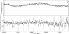 |
Fig. 1. Long-term light curves of GX 9+1 in different energy ranges: 2–20 keV with MAXI (top) and 15–50 keV with BAT (bottom). The arrow indicates the time of the simultaneous IXPE, NuSTAR, NICER, and INTEGRAL observation campaign. |
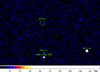 |
Fig. 2. INTEGRAL/IBIS 28–60 keV mosaic image centered on GX 9+1 from data simultaneous with the IXPE observation. The color bar indicates the significance. |
Figure 3 presents the light curves of GX 9+1 as observed by IXPE, NuSTAR, and NICER. The figure also shows the IXPE hardness ratio, defined as the 5–8 keV/3–5 keV flux ratio, and the NuSTAR hard color, calculated as the 10–20 keV/6–10 keV flux ratio. The time bins used are 200 s for NuSTAR and IXPE and 50 s for NICER. Figure 4 highlights the NuSTAR light curves, hardness, and the corresponding CCD. The soft color is defined as the 6–10 keV/3–6 keV flux ratio. It is evident from Fig. 4 that the source moved toward the banana branch during the NuSTAR observation. Based on the CCD values, we divided the data points into two groups to investigate spectral variability. The black upper box (UB; with a soft color > 0.79) includes the harder points in the upper right part of the CCD. Only a few data points fall within this region and correspond to the higher flux peaks in the light curves shown in Fig. 3. This confirms the well-known behavior of GX 9+1, where hardening corresponds to an increase in flux. The spectral parameters of the UB and those of the red lower box (LB; with a soft color < 0.79) both correspond to a banana state and do not differ significantly enough to justify splitting the spectral analysis into two separate parts. Therefore, we combined all data into a single averaged spectrum to improve the S/N.
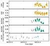 |
Fig. 3. IXPE, NuSTAR (200 s time bins for both), and NICER (50 s time bins) light curves of GX 9+1 (count s−1). The second and fourth panels show the IXPE and NuSTAR hardness-ratios: 5–8 keV/3–5 keV and 10–20 keV/6–10 keV, respectively. Empty gray circles indicate data points that are not simultaneous with the IXPE exposure. |
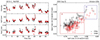 |
Fig. 4. left panel: NuSTAR 3–20 keV light curve, soft color 6–10 keV/3–6 keV and hard color 10–20 keV/6–10 keV of GX 9+1. Right panel: NuSTAR data color-color diagram of GX 9+1. The lower box (LB) and upper box (UB) indicate the data grouped together in the same spectrum. See text for details. |
3.2. Spectral analysis
We performed joint NICER+IXPE+NuSTAR broadband spectral analysis, starting with the NuSTAR spectrum alone, then adding NICER, and finally incorporating the IXPE data at the end of the best-fit procedure. For the simultaneous fitting, we used the complete NuSTAR and IXPE spectra and only the part of the NICER spectra simultaneously with NuSTAR (see Fig. 3).
For interstellar medium (ISM) absorption, we adopted the most recent ISM abundances as described by Wilms et al. (2000). The hydrogen column density, NH, was allowed to vary during the fitting procedure.
We fitted the NuSTAR and NICER spectra with a model composed of an absorbed disk black body (diskbb) plus a Comptonizing component. For the Comptonizing component we used a convolution model (thcomp) applied to the star and/or spreading-layer black body (bbodyrad). Before fitting, we extended the energy vector over which the thcomp model is computed by using the XSPEC command energies 0.01 1000.0 1000 log. Considering the residuals of the fit, we detected a weak iron line around 6.2 keV. We tested a Gaussian component to model the presence of the iron line in our spectral fit. The Akaike Information Criterion (AIC) check indicated a significant improvement in the fit, with a ΔAIC of 12.54, supporting the necessity of this additional component. The AIC quantifies the information loss when using a specific model compared to another (Akaike 1974); Burnham.20043. We also tested a more comprehensive and physical model, RelxillNS, which accounts for the presence of a small reflection component. In this case, the AIC test showed no statistical preference over the simple Gaussian model (ΔAIC = 4.22). However, we chose to use the RelxillNS model despite its low significance and flux contribution, as it offers more detailed insights into the physical parameters. The RelxillNS model package reproduces the relativistic reflection from the innermost regions of an accretion disk (García et al. 2014); Dauser.etAl.2014. Specifically, RelxillNS assumes a single-temperature blackbody spectrum that illuminates the surface of the accretion disk at 45°, which could physically originate from the emission of the spreading layer or NS surface (García et al. 2022). We set the reflection fraction parameter in RelxillNS to a negative value to isolate only the reflected component, as indicated in García et al. (2016). We also linked the temperature of the seed photons to the temperature in the bbodyrad component. We fixed the number density at log(ne) = 18, as reported in García et al. (2016), the emissivity index to the best fit value (qem = 3), the dimensionless spin a of the NS to 0.2, a typical spin frequency (see e.g., Braje et al. 2000).
NICER data revealed residuals below 2.5 keV in the energy spectra, due to features not corrected in the NICER ancillary response file (ARF) (Miller et al. 2013; Strohmayer et al. 2018). To account for this, we included three absorption edges in the NICER data (edge in XSPEC) at 1.5, 1.8, and 2.4 keV, respectively. It should be noted that numerous edges detected in previous observations have also been directly attributed to the source, likely due to the presence of ionized material around the system (Thomas et al. 2023); Iaria.2005.
The joint NICER+IXPE+NuSTAR energy spectrum is shown in Fig. 5. The XSPEC syntax of the model used is: constant*edge*edge*edge*TBabs(diskbb+relxillNS+
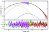 |
Fig. 5. Unfolded spectrum of GX 9+1 as observed by NuSTAR (red and black points), NICER (light green points), and IXPE-I (light blue, magenta and violet points for each DU, respectively). The dotted line indicates the Comptonization component, dashed line shows the disk component, and the solid line represents the reflection. |
thcomp*bbodyrad). Table 2 lists the spectral parameter values obtained from the joint NICER+IXPE+NuSTAR spectral fit. Table 3 reports the cross-calibration constants between the different instruments, determined by setting the NuSTAR FPMA constant to 1, the gain shift of IXPE and the NICER edge values. All table values are reported at the confidence level (CL) 90%, which corresponds to approximately 1.6σ. The normalizations of the diskbb and bbodyrad components are provided assuming a source distance of 10 kpc. The fit yields reasonable values of the spectral parameters for a LMXB hosting a NS as the compact object, and indicates that GX 9+1 is in a banana state observed at a relatively low inclination angle. The low Fe abundance indicates a late-type companion star.
Spectral fitting (Part 1): Model fitting parameters NICER, NuSTAR, and IXPE.
Spectral fitting (Part 2): Cross-calibration constants, IXPE gain shift, NICER absorption edges, unabsorbed photon fluxes, and flux ratios.
The obtained NH value may be overestimated, although it is compatible with previous studies (van den Berg & Homan 2017; Thomas et al. 2023). As reported by Iaria et al. (2005), the BeppoSAX spectra of GX 9+1 show absorption edges due to material in front of the source. To account for variations in iron and oxygen abundances, we applied the Tübingen-Boulder ISM absorption model (TBfeo in XSPEC) to the total emission. However, this model was difficult to constrain to physically acceptable oxygen and iron abundances, likely due to both nonstandard element abundances and the short duration of the simultaneous NICER spectrum. Nevertheless, the other spectral parameters remain consistent regardless of the choice of absorption models.
Additionally, Table 3 provides the flux values of the source in different energy bands, as well as the ratios of the fluxes of the different model components relative to the IXPE bands 2–8 keV and 2–3 keV, respectively. The source luminosity is calculated as L/LEdd = 1.5%, assuming a mass of 1.4 M⊙ and a source distance of 4 kpc (van den Berg & Homan 2017; Iaria et al. 2005). This yields an estimated accretion rate of ṁ ∼ 4.5 × 10⁻¹⁰ M⊙/yr, assuming an accretion efficiency of 0.1.
3.3. Spectro-polarimetric analysis
We first performed an unweighted polarimetric analysis of the entire IXPE observation using IXPEOBSSIM (v.31.0.1; Baldini et al. 2022), with the latest available calibration file (v.13.20240701). Figure 6 shows, for each DU, the normalized Stokes parameters measured by IXPE and obtained using the PCUBE task of IXPEOBSSIM, along with the minimum detectable polarization (MDP) at the 99% level. The black cross represents the combination of the three DU signals, which lies below the 99% MDP. Therefore, we could only provide an upper limit for the PD in the 2–8 keV range, and a value of 3.0 ± 0.9% at 3.1σ in the 2–3 keV.
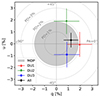 |
Fig. 6. 2–8 keV normalized Stokes q (Q/I) and u (U/I) parameters obtained for the three DUs with the PCUBE algorithm of IXPEOBSSIM (Baldini et al. 2022). The black cross represents the combination of the three DUs, while the gray-filled circle corresponds to the combined 99% MDP. |
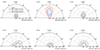 |
Fig. 7. Contour plots of the PD and PA at the 68.3% (1σ), 90% (1.6σ), and 99% CL (2.6σ) obtained with XSPEC at different energy ranges. |
We performed the spectro-polarimetric analysis by adding the polconst convolution model to the total model and applying it to the entire set of IXPE spectra (I, Q and U), the NICER spectrum, and the two NuSTAR spectra. The XSPEC syntax of the model applied is: polconst*constant*edge*edge*edge*Tbabs(diskbb+rel
xillNS+thcomp*bbodyrad). To derive the PD and polarization angle (PA) of the polconst model, we fixed the other spectral parameters of the total model based on those found from spectral fitting (see Table 2). Table 4 presents the results of the XSPEC analysis for PD and PA at different CL, computed with the error command for one parameter of interest. The upper limit is reported at the 99.7% CL (3σ). Figure 7 reports the contours of PD and PA obtained with XSPEC for the IXPE observation in the 2–3, 2–4, 3–4, 3–8, 4–8 and 2–8 keV energy bands. As shown in Fig. 7, the PD between 2–8 keV is compatible with zero polarization above the 68.3% CL (1σ), and consequently the PA is unconstrained. The same result is obtained by studying the PD and PA at different energy intervals, with the exception of the 2–3 keV energy interval. In this case, we found a detection at the 95.5% CL (2σ) in the 2–3 keV range and a hint of detection at the 68.3% CL (1σ) in the 2–4 keV range. Consistent results are also obtained using the model-independent IXPEOBSSIM task as stated at the beginning of this section.
Polarization degree (PD) and angle (PA) values at different energy bands (band) and confidence levels (CL) for a single parameter, as determined with XSPEC.
Based on these results, we also applied polconst to each individual spectral component. The XSPEC syntax of the model used is: constant*edge*edge*edge*TBabs(polconst*diskbb+ polconst*relxillNS+polconst*(thcomp*bbodyrad)). We fixed the PA of the reflection component to the best fit of the Comptonized component, 90°, and allowed the PD values to vary. We obtained an upper limit for the Comptonized component of PD < 5.1% at the 99.7% CL, while the PD of the reflection component remained unconstrained (< 100% at 99.7% CL). The PD of the disk component converges to a value (PD =  %) consistent with that obtained in the 2–3 keV energy range when applying polconst to the entire model, as reported in Table 4. Notably, the best fit PA (PA =
  ) is naturally orthogonal to the fixed PA of Compton and the reflection components, although uncertainties are large. We also attempted to fix the PD of the Comptonization component to the best-fit value of 0.39%, which is a plausible value for low inclination angles (Gnarini et al. 2022), while the PD of the reflection component was fixed at 10% (Lapidus & Sunyaev 1985). As before, we assumed that the PA of the reflection and Comptonized components are aligned in the same direction, fixing the angle to 90°. The fitting procedure again yielded a disk PD value consistent with that obtained in the 2–3 keV energy range when applying polconst to the entire model, with PD–disk =
  % and PA =
  degree (90% CL).
4. Discussion and conclusions
We report on the IXPE observation of GX 9+1, conducted simultaneously with NuSTAR and NICER, and with serendipitous simultaneous INTEGRAL observations. This new observation campaign provides new insights into the polarimetric and spectroscopic properties of this NS-LMXB system. GX 9+1 offers a unique comparison with other similar objects, especially given the differences in polarization behavior observed across atoll and Z-class sources. Previous studies of atoll sources, such as GX 9+9 and GS 1826–238, have highlighted low PDs, with GX 9+9 showing a PD of ∼2%, attributed to a combination of boundary layer (BL) and reflection effects (Ursini et al. 2023), and GS 1826–238 displaying only a strict upper limit of less than 1.3% in the 2–8 keV range. For GX 9+1, our results demonstrate that the PD is modest, less than ≃1.9% in 2–8 keV, similar to GS 1826–238, Ser X–1, and GX 3+1, and consistent with expectations for systems with low inclination angles.
The broadband spectrum of GX 9+1 can be described by a soft thermal component and a harder Comptonized emission, with spectral parameters characteristic of an atoll source in the soft state. Faint reflection features are also present in the spectrum, but their contribution to the total flux is very low (≃2%). Although the reflection component is likely highly polarized (Lapidus & Sunyaev 1985), it does not contribute significantly to the total PD. The spectrum is predominantly dominated by Compton emission, accounting for approximately 57% of the total flux, while roughly 41% of the flux is due to the disk emission.
The PD measured in the 2–8 keV band, of < 1.9%, is consistent with previous findings for other atoll sources, where the PD typically does not exceed 2%, except in cases where a significant Comptonized component, together with a reflection component, dominates the emission (e.g., the steep increase in PD between 7–8 keV in 4U 1820–30; Di Marco et al. 2023a) or the source is viewed at a high inclination angle (see for example the dipping source 4U 1624–49; Saade et al. 2024; Gnarini et al. 2024b).
We report a marginal detection in the 2–3 keV energy range at the 90% CL (see Fig. 7 and Table 4). In this lower energy range (2–3 keV), the disk emission represents 70% of the total emission, while the remaining 30% is mostly due to the Comptonization component. Our results indicate that most of the PD detected between 2–3 keV is due to disk emission. Indeed, applying the constant polarization model to each component (see Sect. 3.3), the PD of the disk converges to a value compatible with the marginal detection found between 2–3 keV, and the best-fit PA naturally converges to 90 degrees with respect to the Comptonized and reflection PA. Although the PD value found is relatively high for a standard accretion disk modeled as a semi-infinite plane-parallel atmosphere (Chandrasekhar 1960), the 90% uncertainty remains large.
Moreover, as reported by Gnarini et al. (2022), simulations considering the shell geometry for the corona show an increase in PD below 3 keV. While this increase is most evident for inclinations higher than those found in our analysis (> 40°), our results are consistent within the uncertainties. The inclination angle of GX 9+1 remains a subject of debate. However, our results estimate a relatively low inclination of the source, 23° < i < 46° (see Table 2), which likely affects the overall PD and agrees with the upper limit obtained. As observed in sources such as Ser X-1 and GX 9+9, the disk inclination and the geometry of the Comptonizing region are key factors in determining the polarization properties. The detection of polarization at the 90% CL suggests that longer observations of GX 9+1 with IXPE, possibly in conjunction with other observatories like NICER or NuSTAR, could yield a significant polarization signal, help clarify its nature, and refine the models used to interpret these data. Insights from polarimetric observations will also be crucial for understanding the connection between spectral states and the geometric configurations of these systems.
Moreover, as shown in Table 2, the covering factor of the Comptonized component is relatively low (∼0.5). This can be explained within the scenario outlined by the spectro-polarimetric analysis. Specifically, the low inclination obtained from the spectral fit, together with the low polarization and low covering factor, can be explained if the spreading layer is the site of Comptonization of the NS seed photons. Observing the source at a low inclination allows us to have a direct view of the NS pole.
The model with the smallest AIC (AIC = 2 × n + χ2) is preferred, where n is the number of free parameters in the fit. Generally, a difference of ΔAIC > 10 indicates a large and statistically significant improvement in the fit, and the model with the lower AIC have to be considered substantially better. For 4 ≤ ΔAIC ≤ 7, the difference is not large enough to be considered conclusive. In this range, there is some evidence favoring one model, but the improvement is not substantial (Burnham & Anderson 2004).
Acknowledgments
This work reports observations obtained with the Imaging X-ray Polarimetry Explorer (IXPE), a joint US (NASA) and Italian (ASI) mission, led by Marshall Space Flight Center (MSFC). The research uses data products provided by the IXPE Science Operations Center (MSFC), using algorithms developed by the IXPE Collaboration, and distributed by the High-Energy Astrophysics Science Archive Research Center (HEASARC). AT, FC, and SF acknowledge financial support by the Istituto Nazionale di Astrofisica (INAF) grant 1.05.23.05.06: “Spin and Geometry in accreting X-ray binaries: The first multi frequency spectro-polarimetric campaign”. AG, FC, SB, SF, GM, PF and FU acknowledge financial support by the Italian Space Agency (Agenzia Spaziale Italiana, ASI) through the contract ASI-INAF-2022-19-HH.0. SF, PS have been also supported by the project PRIN 2022 – 2022LWPEXW – “An X-ray view of compact objects in polarized light”, CUP C53D23001180006. MN is a Fonds de Recherche du Quebec – Nature et Technologies (FRQNT) postdoctoral fellow. JP thanks the Academy of Finland grant 333112 for support. This research used data products and software provided by the IXPE, the NICER, and NuSTAR teams and distributed with additional software tools by the High-Energy Astrophysics Science Archive Research Center (HEASARC), at NASA Goddard Space Flight Center.
References
- Akaike, H. 1974, IEEE Trans. Autom. Control, AC-19, 716 [Google Scholar]
- Anitra, A., Gnarini, A., Di Salvo, T., et al. 2025, A&A, 697, A83 [NASA ADS] [CrossRef] [EDP Sciences] [Google Scholar]
- Arnaud, K. A. 1996, in Astronomical Data Analysis Software and Systems V, eds. G. H. Jacoby, & J. Barnes (San Francisco: Astron. Soc. Pac.), ASP Conf. Ser., 101, 17 [NASA ADS] [Google Scholar]
- Baldini, L., Bucciantini, N., Lalla, N. D., et al. 2022, SoftwareX, 19, 101194 [NASA ADS] [CrossRef] [Google Scholar]
- Braje, T. M., Romani, R. W., & Rauch, K. P. 2000, ApJ, 531, 447 [Google Scholar]
- Burnham, K. P., & Anderson, D. R. 2004, Sociol. Methods Res., 33, 261 [Google Scholar]
- Capitanio, F., Fabiani, S., Gnarini, A., et al. 2023, ApJ, 943, 129 [NASA ADS] [CrossRef] [Google Scholar]
- Chandrasekhar, S. 1960, Radiative Transfer (New York: Dover Publications) [Google Scholar]
- Cocchi, M., Gnarini, A., Fabiani, S., et al. 2023, A&A, 674, L10 [NASA ADS] [CrossRef] [EDP Sciences] [Google Scholar]
- Costa, E., Soffitta, P., Bellazzini, R., et al. 2001, Nature, 411, 662 [NASA ADS] [CrossRef] [Google Scholar]
- Courvoisier, T. J. L., Walter, R., Beckmann, V., et al. 2003, A&A, 411, L53 [NASA ADS] [CrossRef] [EDP Sciences] [Google Scholar]
- Dauser, T., Garcia, J., Parker, M. L., Fabian, A. C., & Wilms, J. 2014, MNRAS, 444, L100 [Google Scholar]
- Di Marco, A., Costa, E., Muleri, F., et al. 2022, AJ, 163, 170 [NASA ADS] [CrossRef] [Google Scholar]
- Di Marco, A., La Monaca, F., Poutanen, J., et al. 2023a, ApJ, 953, L22 [NASA ADS] [CrossRef] [Google Scholar]
- Di Marco, A., Soffitta, P., Costa, E., et al. 2023b, AJ, 165, 143 [CrossRef] [Google Scholar]
- Di Salvo, T., Papitto, A., Marino, A., Iaria, R., & Burderi, L. 2024, in Handbook of X-ray and Gamma-ray Astrophysics, eds. C. Bambi, & A. Santangelo (Singapore: Springer), 4031 [CrossRef] [Google Scholar]
- Done, C., Gierliński, M., & Kubota, A. 2007, A&A Rev., 15, 1 [CrossRef] [Google Scholar]
- Fabiani, S., Capitanio, F., Iaria, R., et al. 2024, A&A, 684, A137 [NASA ADS] [CrossRef] [EDP Sciences] [Google Scholar]
- Farinelli, R., Fabiani, S., Poutanen, J., et al. 2023, MNRAS, 519, 3681 [NASA ADS] [CrossRef] [Google Scholar]
- Fridriksson, J. K., Homan, J., & Remillard, R. A. 2015, ApJ, 809, 52 [Google Scholar]
- García, J., Dauser, T., Lohfink, A., et al. 2014, ApJ, 782, 76 [Google Scholar]
- García, J. A., Fabian, A. C., Kallman, T. R., et al. 2016, MNRAS, 462, 751 [Google Scholar]
- García, J. A., Dauser, T., Ludlam, R., et al. 2022, ApJ, 926, 13 [CrossRef] [Google Scholar]
- Gendreau, K. C., Arzoumanian, Z., Adkins, P. W., et al. 2016, in Space Telescopes and Instrumentation 2016: Ultraviolet to Gamma Ray, eds. J. W. A. den Herder, T. Takahashi, & M. Bautz, Proc. SPIE, 9905, 99051H [NASA ADS] [CrossRef] [Google Scholar]
- Gierlinski, M., & Done, C. 2002, MNRAS, 331, L47 [CrossRef] [Google Scholar]
- Gnarini, A., Ursini, F., Matt, G., et al. 2022, MNRAS, 514, 2561 [NASA ADS] [CrossRef] [Google Scholar]
- Gnarini, A., Farinelli, R., Ursini, F., et al. 2024a, A&A, 692, A123 [NASA ADS] [CrossRef] [EDP Sciences] [Google Scholar]
- Gnarini, A., Lynne Saade, M., Ursini, F., et al. 2024b, A&A, 690, A230 [NASA ADS] [CrossRef] [EDP Sciences] [Google Scholar]
- Harrison, F. A., Craig, W. W., Christensen, F. E., et al. 2013, ApJ, 770, 103 [Google Scholar]
- Hasinger, G., & van der Klis, M. 1989, A&A, 225, 79 [NASA ADS] [Google Scholar]
- Homan, J., van der Klis, M., Wijnands, R., et al. 2007, ApJ, 656, 420 [NASA ADS] [CrossRef] [Google Scholar]
- Iaria, R., di Salvo, T., Robba, N. R., et al. 2005, A&A, 439, 575 [NASA ADS] [CrossRef] [EDP Sciences] [Google Scholar]
- Iaria, R., Mazzola, S. M., Di Salvo, T., et al. 2020, A&A, 635, A209 [NASA ADS] [CrossRef] [EDP Sciences] [Google Scholar]
- Kaastra, J. S., & Bleeker, J. A. M. 2016, A&A, 587, A151 [NASA ADS] [CrossRef] [EDP Sciences] [Google Scholar]
- La Monaca, F., Di Marco, A., Poutanen, J., et al. 2024, ApJ, 960, L11 [NASA ADS] [CrossRef] [Google Scholar]
- Langmeier, A., Sztajno, M., Truemper, J., & Hasinger, G. 1985, Space Sci. Rev., 40, 367 [Google Scholar]
- Lapidus, I. I., & Sunyaev, R. A. 1985, MNRAS, 217, 291 [NASA ADS] [CrossRef] [Google Scholar]
- Lebrun, F., Leray, J. P., Lavocat, P., et al. 2003, A&A, 411, L141 [NASA ADS] [CrossRef] [EDP Sciences] [Google Scholar]
- Lin, D., Remillard, R. A., & Homan, J. 2007, ApJ, 667, 1073 [CrossRef] [Google Scholar]
- Lin, D., Remillard, R. A., & Homan, J. 2009, ApJ, 696, 1257 [NASA ADS] [CrossRef] [Google Scholar]
- Miller, J. M., Parker, M. L., Fuerst, F., et al. 2013, ApJ, 779, L2 [NASA ADS] [CrossRef] [Google Scholar]
- Muno, M. P., Remillard, R. A., & Chakrabarty, D. 2002, ApJ, 568, L35 [NASA ADS] [CrossRef] [Google Scholar]
- Neronov, A., Savchenko, V., Tramacere, A., et al. 2021, A&A, 651, A97 [NASA ADS] [CrossRef] [EDP Sciences] [Google Scholar]
- Paizis, A., Ebisawa, K., Tikkanen, T., et al. 2005, A&A, 443, 599 [CrossRef] [EDP Sciences] [Google Scholar]
- Piconcelli, E., Jimenez-Bailón, E., Guainazzi, M., et al. 2004, MNRAS, 351, 161 [Google Scholar]
- Saade, M. L., Kaaret, P., Gnarini, A., et al. 2024, ApJ, 963, 133 [NASA ADS] [CrossRef] [Google Scholar]
- Schnerr, R. S., Reerink, T., van der Klis, M., et al. 2003, A&A, 406, 221 [NASA ADS] [CrossRef] [EDP Sciences] [Google Scholar]
- Soffitta, P., Baldini, L., Bellazzini, R., et al. 2021, AJ, 162, 208 [CrossRef] [Google Scholar]
- Strohmayer, T. E., Gendreau, K. C., Altamirano, D., et al. 2018, ApJ, 865, 63 [NASA ADS] [CrossRef] [Google Scholar]
- Thomas, N. T., Gudennavar, S. B., & Bubbly, S. G. 2023, MNRAS, 525, 2355 [NASA ADS] [CrossRef] [Google Scholar]
- Ubertini, P., Lebrun, F., Di Cocco, G., et al. 2003, A&A, 411, L131 [CrossRef] [EDP Sciences] [Google Scholar]
- Ursini, F., Farinelli, R., Gnarini, A., et al. 2023, A&A, 676, A20 [NASA ADS] [CrossRef] [EDP Sciences] [Google Scholar]
- Ursini, F., Gnarini, A., Bianchi, S., et al. 2024, A&A, 690, A200 [NASA ADS] [CrossRef] [EDP Sciences] [Google Scholar]
- van den Berg, M., & Homan, J. 2017, ApJ, 834, 71 [Google Scholar]
- van der Klis, M. 2006, in Compact stellar X-ray sources, eds. W. Lewin, & M. van der Klis (Cambridge: Cambridge University Press), Camb. Astrophys. Ser., 39, 39 [NASA ADS] [CrossRef] [Google Scholar]
- Weisskopf, M. C., Soffitta, P., Baldini, L., et al. 2022, JATIS, 8, 1 [Google Scholar]
- Weisskopf, M. C., Soffitta, P., Ramsey, B. D., et al. 2023, Nat. Astron., 7, 635 [NASA ADS] [CrossRef] [Google Scholar]
- Wilms, J., Allen, A., & McCray, R. 2000, ApJ, 542, 914 [Google Scholar]
All Tables
Spectral fitting (Part 2): Cross-calibration constants, IXPE gain shift, NICER absorption edges, unabsorbed photon fluxes, and flux ratios.
Polarization degree (PD) and angle (PA) values at different energy bands (band) and confidence levels (CL) for a single parameter, as determined with XSPEC.
All Figures
|
Fig. 1. Long-term light curves of GX 9+1 in different energy ranges: 2–20 keV with MAXI (top) and 15–50 keV with BAT (bottom). The arrow indicates the time of the simultaneous IXPE, NuSTAR, NICER, and INTEGRAL observation campaign. |
| In the text | |
|
Fig. 2. INTEGRAL/IBIS 28–60 keV mosaic image centered on GX 9+1 from data simultaneous with the IXPE observation. The color bar indicates the significance. |
| In the text | |
|
Fig. 3. IXPE, NuSTAR (200 s time bins for both), and NICER (50 s time bins) light curves of GX 9+1 (count s−1). The second and fourth panels show the IXPE and NuSTAR hardness-ratios: 5–8 keV/3–5 keV and 10–20 keV/6–10 keV, respectively. Empty gray circles indicate data points that are not simultaneous with the IXPE exposure. |
| In the text | |
|
Fig. 4. left panel: NuSTAR 3–20 keV light curve, soft color 6–10 keV/3–6 keV and hard color 10–20 keV/6–10 keV of GX 9+1. Right panel: NuSTAR data color-color diagram of GX 9+1. The lower box (LB) and upper box (UB) indicate the data grouped together in the same spectrum. See text for details. |
| In the text | |
|
Fig. 5. Unfolded spectrum of GX 9+1 as observed by NuSTAR (red and black points), NICER (light green points), and IXPE-I (light blue, magenta and violet points for each DU, respectively). The dotted line indicates the Comptonization component, dashed line shows the disk component, and the solid line represents the reflection. |
| In the text | |
|
Fig. 6. 2–8 keV normalized Stokes q (Q/I) and u (U/I) parameters obtained for the three DUs with the PCUBE algorithm of IXPEOBSSIM (Baldini et al. 2022). The black cross represents the combination of the three DUs, while the gray-filled circle corresponds to the combined 99% MDP. |
| In the text | |
|
Fig. 7. Contour plots of the PD and PA at the 68.3% (1σ), 90% (1.6σ), and 99% CL (2.6σ) obtained with XSPEC at different energy ranges. |
| In the text | |
Current usage metrics show cumulative count of Article Views (full-text article views including HTML views, PDF and ePub downloads, according to the available data) and Abstracts Views on Vision4Press platform.
Data correspond to usage on the plateform after 2015. The current usage metrics is available 48-96 hours after online publication and is updated daily on week days.
Initial download of the metrics may take a while.