| Issue |
A&A
Volume 684, April 2024
|
|
|---|---|---|
| Article Number | A31 | |
| Number of page(s) | 25 | |
| Section | Extragalactic astronomy | |
| DOI | https://doi.org/10.1051/0004-6361/202347826 | |
| Published online | 29 March 2024 | |
The Lockman–SpReSO project
Galactic flows in a sample of far-infrared galaxies
1
Instituto de Astrofísica de Canarias, 38205 La Laguna, Tenerife, Spain
e-mail: This email address is being protected from spambots. You need JavaScript enabled to view it.
; This email address is being protected from spambots. You need JavaScript enabled to view it.
2
Departamento de Astrofísica, Universidad de La Laguna (ULL), 38205 La Laguna, Tenerife, Spain
3
Fundación Galileo Galilei-INAF, Rambla José Ana Fernández Pérez, 7, 38712 Breña Baja, Tenerife, Spain
4
Asociación Astrofísica para la Promoción de la Investigación, Instrumentación y su Desarrollo, ASPID, 38205 La Laguna, Tenerife, Spain
5
Instituto de Física de Cantabria (CSIC-Universidad de Cantabria), 39005 Santander, Spain
6
Centro de Astrobiología (CSIC/INTA), 28692 ESAC Campus, Villanueva de la Cañada, Madrid, Spain
7
Instituto de Astronomía, Universidad Nacional Autónoma de México, Apdo. Postal 70-264, 04510 Ciudad de México, Mexico
8
Institut de Radioastronomie Millimétrique (IRAM), Av. Divina Pastora 7, Núcleo Central, 18012 Granada, Spain
9
Departamento de Física de la Tierra y Astrofísica, Instituto de Física de Partículas y del Cosmos, IPARCOS, Universidad Complutense de Madrid (UCM), 28040 Madrid, Spain
10
ISDEFE for European Space Astronomy Centre (ESAC)/ESA, PO Box 78 28690 Villanueva de la Cañada, Madrid, Spain
11
Astronomical Observatory Institute, Faculty of Physics, Adam Mickiewicz University, ul. Słoneczna 36, 60-286 Poznań, Poland
12
Space Science and Geospatial Institute (SSGI), Entoto Observatory and Research Center (EORC), Astronomy and Astrophysics Research Division, PO Box 33679 Addis Abbaba, Ethiopia
13
Instituto de Astrofísica de Andalucía (CSIC), 18080 Granada, Spain
14
Physics Department, Mbarara University of Science and Technology (MUST), Mbarara, Uganda
Received:
29
August
2023
Accepted:
8
January
2024
Abstract
Context. The Lockman–SpReSO project is an optical spectroscopic survey of 956 far-infrared (FIR) objects within the Lockman Hole field limited by magnitude RC(AB) < 24.5. Fe II and Mg II absorption lines have been detected in 21 out of 456 objects with a determined spectroscopic redshift in the catalogue. The redshifts of these objects are in the range 0.5 ≲ z ≲ 1.44.
Aims. The aim of this study is to investigate material ejection from star-forming regions and material infall into galaxies by analysing the Fe II and Mg II absorption lines. Additionally, we explore whether the correlations found in previous studies between these galactic wind velocities, line equivalent widths (EWs), and galaxy properties such as stellar mass (M*), star formation rate (SFR), and specific star formation rate (sSFR) are valid for a sample with FIR-selected objects. The objects analysed span an M* range of 9.89 < log(M*/M⊙) < 11.50 and an SFR range of 1.01 < log(SFR) < 2.70.
Methods. We performed measurements of the Mg IIλλ2796, 2803, Mg Iλ2852, Fe IIλλ2374, 82, Fe IIλλ2586, 2600, and Fe IIλ2344 spectral lines present in the spectra of the selected sample to determine the EW and velocity of the flows observed in the star-forming galaxies. Subsequently, we conducted 107 bootstrap simulations using the Spearman’s rank correlation coefficient (ρs) to explore correlations with galaxy properties. Furthermore, we calculated the covering factor, gas density, and optical depth for the measured Fe II doublets.
Results. Our analysis reveals strong correlations between the EW of Mg II lines and both M* (ρs = 0.43, 4.5σ) and SFR (ρs = 0.42, 4.4σ). For the Fe II lines, we observed strong correlations between the EW and SFR (ρs ∼ 0.65, > 3.9σ), with a weaker correlation for M* (ρs ∼ 0.35, > 1.9σ). No notable correlations were found between velocity measurements of the Mg II line and M*, SFR, or sSFR of the objects (ρs ∼ 0.1). However, a strong negative correlation was found between the velocity of the Fe II lines and the SFR of the galaxies (ρs ∼ −0.45, ∼3σ). Our results align with those of previous studies, although only FIR-selected objects are investigated here. Finally, we detect a candidate ‘loitering outflow’, a recently discovered subtype of the iron low-ionisation broad absorption line (FeLoBAL) quasars, at a redshift of z = 1.4399, exhibiting emission in C III] and low line velocities (|v|≲200 km s−1).
Key words: techniques: spectroscopic / galaxies: evolution / galaxies: starburst / galaxies: statistics
© The Authors 2024
 Open Access article, published by EDP Sciences, under the terms of the Creative Commons Attribution License (https://creativecommons.org/licenses/by/4.0), which permits unrestricted use, distribution, and reproduction in any medium, provided the original work is properly cited.
This article is published in open access under the Subscribe to Open model. This email address is being protected from spambots. You need JavaScript enabled to view it. to support open access publication.
1. Introduction
To understand how galaxies evolve, we need to study the processes that galaxies undergo over time. Galactic winds are one of the mechanisms that play a fundamental role in their evolution. When giant stars explode as supernovae, they eject material enriched in heavy elements into the galactic halo, enriching the intergalactic medium through a mechanism known as galactic winds (Veilleux et al. 2005). Subsequently, this ejected material can be reaccreted by the gravitational potential of the host galaxy, leading to a ‘reinjection’, or inflow, of enriched material to refuel the galaxy and trigger the birth of the new generation of stars. The study of this material cycle is a major challenge in cosmology (Péroux & Howk 2020). Investigation of the frequency with which this cycle occurs, its characteristics, and its dependence on host galaxy properties, such as stellar mass (M*) or star formation rate (SFR), will help us to better understand the dynamical and chemical evolution of the galaxies, the circumgalactic medium, and the intergalactic medium (Tumlinson et al. 2017; Veilleux et al. 2020).
Studies of galactic outflows have shown that this phenomenon is a common feature of star-forming galaxies (SFGs) across cosmic time. In the local Universe, Chen et al. (2010) showed the ubiquity of outflows in galaxies with a high SFR. Martin et al. (2012) found winds in about half of their sample of approximately 200 objects with redshifts between 0.4 and 1.4. These authors found no relationship between the rate of detection of outflows and the physical properties of galaxies, but reported a strong relationship with the viewing angle, strengthening the idea of the presence of biconical outflows in SFGs.
The kinematics of galactic winds allow them to be studied in the spectrum of their host galaxy. The spectral lines produced by the flow itself are blueshifted (redshifted) in cases where the material is ejected (captured) by the galaxy. Studies were therefore carried out on individual objects to look for properties of the flows and their possible dispersion (Martin et al. 2012; Erb et al. 2012; Rubin et al. 2014; Chisholm et al. 2015; Finley et al. 2017a,b; Prusinski et al. 2021; Xu et al. 2022; Davis et al. 2023, among others), and on coadded spectra of similar objects to look for general properties of galactic flows (Weiner et al. 2009; Rubin et al. 2010; Erb et al. 2012; Zhu et al. 2015; Prusinski et al. 2021, among others). This latter approach is useful for distant objects where the signal-to-noise ratio is poor, as it enables the acquisition of generalised information from the whole sample, although unique properties of each individual object may be forfeited.
Many studies have focused on the analysis of low-ionisation resonant absorption spectral lines. Optical features such as Ca IIλλ3933, 69 or Na Iλλ5890, 96 (Martin 2005; Chen et al. 2010) are useful because of their presence in low-redshift SFGs. There are other interesting low-ionisation absorption lines in the UV range that are becoming available to ground observations for objects at redshifts z ≳ 0.3. The Mg IIλλ2796, 2803 doublet is one of the most widely used (Weiner et al. 2009; Erb et al. 2012; Rubin et al. 2014; Zhu et al. 2015; Finley et al. 2017a; Prusinski et al. 2021) because it is the most common ionised state of magnesium under a wide range of environmental conditions and also has a large oscillator strength. At bluer wavelengths, the Fe II lines (Fe IIλ2344, Fe IIλλ2586, 2600, Fe IIλλ2374, 82) are found to confer an advantage in that they are less sensitive to emission filling (Erb et al. 2012; Martin et al. 2012; Rubin et al. 2014; Zhu et al. 2015; Finley et al. 2017a; Prusinski et al. 2021). For the study of more distant objects, far-UV transitions such as Si II, Al II, C II, C IV, and Lyα, are commonly used to the study of outflows (Shapley et al. 2003; Steidel et al. 2010; Jones et al. 2012; Leclercq et al. 2020, among others).
One of the properties of the outflows derived from the analysis of the spectral lines is the velocity difference between the outflow and the host galaxy. Some studies have found that the velocity of the outflows tends to increase with M* and the SFR of the host galaxy (Martin 2005; Rupke et al. 2005a; Weiner et al. 2009; Chisholm et al. 2015), implying that galaxies with higher SFRs have more energy to eject material via supernovae and also contain a greater amount of material. However, this correlation has not been found in other studies, where the outflow velocity is found to be independent of M* or the SFR of the host galaxy (Rupke et al. 2005b; Chen et al. 2010; Martin et al. 2012; Rubin et al. 2014; Prusinski et al. 2021). These correlations show a significant intrinsic scatter (σ ∼ 0.2 dex, Chisholm et al. 2015; Heckman et al. 2015), meaning that large samples of objects must be studied with a wide range of analysed parameters. Davis et al. (2023) discovered a scatter that is half of that obtained by these latter, previous studies, resulting in a large sample that spans almost three orders of magnitude in M* and SFR. In their study of a sample with a wide range of M* (log M* ∼ 6 − 10 M⊙) and SFR (log SFR ∼ 0.01 − 100 M⊙ yr−1), Xu et al. (2022) found a correlation of high significance between outflow velocity and both SFR and M*.
Most studies that investigate the correlations between galaxy properties and outflow properties tend to focus on normal SFGs. Furthermore, for distant objects (z > 0.5), SFGs are selected based on the UV emission observed in the optical range, which introduces a bias towards a specific type of object. Therefore, it is crucial to conduct studies on objects selected using different criteria. In the paper of Banerji et al. (2011), the authors analyse a sample of 19 submillimetre galaxies and 21 submillimetre faint radio galaxies with an average redshift of z ∼ 1.3. A correlation was found between the velocity of the outflows and SFR, which is consistent with the results seen for lower redshift Ultra-Luminous Infrared Galaxies (ULIRGs).
In the present paper, we describe how we identified and analysed the galactic flows of objects within the framework of the Lockman–SpReSO project Gonzalez-Otero et al. (2023). We used a sample of IR-selected SFGs with Fe II and Mg II absorption lines in their spectra. We fitted these lines to determine the EW and the velocity of the flow relative to that of the system. We explore the correlation between these line properties and the physical parameters of the host galaxies using the flow data from Lockman–SpReSO, Rubin et al. (2014, hereafter RU14) and Prusinski et al. (2021, hereafter PR21) together. In addition to creating a statistically significant set of objects (∼200), we include SFGs chosen for their far-infrared (FIR) brightness, which complements the sample. This is important, as studies of flow in IR-selected distant objects are limited, and such studies are usually carried out on a composite spectrum that lacks the individual properties of the objects. We also determine the covering factor, optical depth, and ion densities for the Fe II doublets.
This is the second paper in the Lockman–SpReSO project series and is structured as follows. In Sect. 2, we describe the sample, the selection criteria, and the comparison samples. In Sect. 3, we describe the flow properties and Sect. 3 shows the line-fitting process. In Sect. 4, we describe the analysis of the correlations between flow and galaxy properties. In Sects. 4.1 and 4.2, we describe our analysis of the EWs and velocities of the flows, respectively, and in Sect. 4.3, we describe our study of the local covering factor, optical depths, and ion densities. Our results and conclusions are summarised in Sect. 5. Magnitudes in the AB system (Oke & Gunn 1983) are used throughout the paper. The cosmological parameters adopted in this work are: ΩM = 0.3, ΩΛ = 0.7, and H0 = 70 km s−1 Mpc−1. Both the SFR and M* assume a Chabrier (2003) initial mass function (IMF).
2. Sample selection and description
2.1. Lockman–SpReSO data
The galaxies studied in this paper have been selected from the Lockman–SpReSO project object catalogue. Detailed description of the observations, reduction and catalogue compilation can be found in the presentation paper Gonzalez-Otero et al. (2023). In summary, the Lockman–SpReSO project focuses on a spectroscopic follow-up of 956 objects selected from FIR observations of the Lockman Hole field with the Herschel Space Observatory, plus a sample of 188 interesting objects in the field, with a sample limiting magnitude in the Cousins R band of RC < 24.5. The spectroscopic observations were made with the WHT/A2F-WYFFOS1(Domínquez Palmero et al. 2014) and WYIN/HYDRA2 instruments for the bright subset of the catalogue (RC < 20.6 mag) and with the GTC/OSIRIS3 instrument (Cepa et al. 2000) for the faint subset (RC > 20 mag). The objects studied here belong to the faint subset, where the resolving power used (R ≡ λ/δλ, δλ being the spectral resolution at wavelength λ) was R = 500 (∼4 Å pix−1) for the blue grism with a FWHM resolution at the central wavelength of 560 km s−1, covering the electromagnetic spectra from 3600 Å to 7200 Å. Two different red grisms were used with R = 500 and R = 1000 (∼3 Å pix−1) and a FWHM resolution at the central wavelength of 511 km s−1 and 267 km s−1, respectively, covering from ∼5000 Å to 10 000 Å. The spectral analysis made it possible to determine the spectroscopic redshift for 456 objects.
The objects for this work were selected by visual inspection among those with a spectroscopic redshift obtained in the framework of the Lockman–SpReSO project, and which also had the Mg IIλλ2796, 2803 doublet in emission or absorption along with some of the Fe II lines in the near-UV range. The observations cover a wavelength that establishes the minimum redshift of the objects we could study. Objects having these properties can only be studied at redshifts greater than 0.4.. A total of 21 objects were selected in which both the Mg IIλλ2796, 2803 doublet and the Fe II lines were found. In all of them, the absorption Fe IIλλ2586, 2600 doublet was detected; in 19 of them, the Mg IIλλ2796, 2803 doublet was found in absorption, and in the remaining two, one (ID 206641), showed a total emission component and the other (ID 120237) both emission and absorption components. Other UV absorption lines were also measured in this study; the Mg Iλ2852 was detected in 15 objects, the Fe IIλλ2374, 82 doublet was detected in 11 objects, and the Fe IIλ2344 line was detected in seven of them.
The sample spans the spectroscopic redshift range between 0.5 and 1.44 (see Table 1). For the determination and study of the galactic flows, it is important to have a good determination of the velocity of the object or, in essence, a good determination of the redshift. All the selected objects show strong emission in the [O II] λλ3726, 29 doublet. This emission is normally produced in the photoionised gas near the star-forming regions, so this is a good determinant of the velocity of the system. Other emission lines, such as the most intense Balmer lines (Hα, Hβ and Hγ), available for the lower redshift objects, or the [O III] λλ4959, 5007, were also used to determine the systemic velocity (or redshift).
Basic information on the objects selected from the Lockman–SpReSO catalogue, ordered by increasing redshift.
Using the selection criteria described above, the selected sample could be contaminated by AGNs, because this type of object can also show emission or absorption in both Mg II and Fe II lines. We used the classification performed by Gonzalez-Otero et al. (in prep.), in which the objects in the Lockman–SpReSO project catalogue were divided into SFGs and AGNs, using different photometric and spectroscopic criteria. For the former, the X-ray-to-optical flux ratio (Szokoly et al. 2004), the X-ray total luminosity (Luo et al. 2017), near-infrared (NIR) and FIR data (Donley et al. 2012; Messias et al. 2012) were used. For the spectroscopic ones, the BPT (Baldwin et al. 1981), the Cid Fernandes et al. (2011) diagrams, and visual inspection were used. With these criteria, objects 120237, 206641, and 206679 were classified as AGNs.
Basic properties of the galaxies were retrieved from the work of Gonzalez-Otero et al. (2023) and compiled here in Table 1. They used their spectroscopic redshift determinations to perform SED fits of the UV to FIR photometric data using the CIGALE software (Code Investigating GALaxy Emission, Burgarella et al. 2005, Boquien et al. 2019), providing more accurate measurements of M* and the total infrared luminosity (LTIR) of the objects than that provided by conventional photometric redshifts. The CIGALE parameter configuration is shown in the Appendix B of Gonzalez-Otero et al. (2023). The M* of the objects samples the range 9.89 < log(M*/M⊙) < 11.50 and the LTIR values are in a range value between 10.84 < log(LTIR/L⊙) < 12.53, with 18 objects compatible with Luminous Infrared Galaxies (LIRGs) and two others compatible with ULIRGs. The individual cutouts of the objects and their SED fittings obtained in the framework of Gonzalez-Otero et al. (2023) are compiled in Appendix A.
The SFR and metallicity of these objects were also obtained from the work of Gonzalez-Otero et al. (in prep.). The SFR of the Lockman–SpReSO project galaxies were studied using the flux of the Balmer lines, LTIR, and the [O II] doublet flux as tracers. In Fig. 1 we have compared the complete Lockman–SpReSO sample with the spectroscopic redshift determined by Gonzalez-Otero et al. (2023) with the sample of objects selected in this paper with absorption in Mg II and Fe II and classified as SFG.
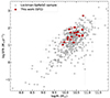 |
Fig. 1. SFR versus M* of the SFGs selected for this study (red) compared to the Lockman–SpReSO sample (grey). The galaxies exhibiting Mg II and Fe II absorption lines populate the region with the highest density of objects in the parent sample. |
The metallicity was analysed following several criteria, although because of the redshift range of the objects studied in this paper only four of them have a metallicity measurement available. Studies such as Pettini & Pagel (2004) and Pilyugin & Grebel (2016), which use spectral lines over the whole optical range, can be applied to only one of the objects in the sample (ID 123207). Studies based on the R23 method, such as Tremonti et al. (2004) and Kobulnicky & Kewley (2004), which use the blue lines in the optical spectrum, can be applied to four of the objects studied. The SFRs collected in Table 1 were obtained using LTIR, the calibration of Kennicutt & Evans (2012) and the IMF of Chabrier (2003). The metallicities given in Table 1 were obtained using the calibration of Tremonti et al. (2004) and the errors are estimated using Monte Carlo simulations.
In Fig. 2 we show the basic properties (M*, redshift, SFR, and sSFR) of the objects from Lockman–SpReSO (blue data), together with data from papers that have also carried outflow studies in SFG (see Sect. 2.2 for a detailed description).
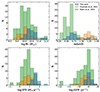 |
Fig. 2. Main properties of the studied objects. The blue bars represent the objects from Lockman–SpReSO survey, the orange bars represent the objects from PR21 and the green bars are the objects from RU14. The top left panel shows the M* of the objects, the top right shows the spectroscopic redshift, the bottom left shows the SFR and, the bottom right shows the sSFR. |
2.2. The comparison samples
In order to have a frame of reference with which to compare, we have included in our work samples from other papers that have studied the galaxy winds produced in SFG.
The numerous sample of 105 galaxies from RU14 was used. They selected objects from existing spectroscopic catalogues for which HST deep observations are available in order to study the morphology, orientation, and spatial distribution of the star formation. They selected objects with redshifts z > 0.3 to ensure Mg II coverage and with B-band magnitude < 23. The M* and the SFR were obtained from a SED fitting procedure in the wavelength range between 2400 Å and 24 μm assuming the IMF of Chabrier (2003). The EW of the lines were derived using the feature-finding algorithm outlined in Cooksey et al. (2008). To normalise the line doublets for the study, the authors used continuum windows located in proximity to the lines region. To determine the flow velocity, two models were used to fit the lines: one with a single component per line and another with two components per line to separate the systemic component at zero velocity from the flow component. The profile of the lines was fitted using a Voigt shape. Additionally, the maximum flow velocity was also determined. To compare with the data obtained from the Lockman–SpReSO objects, we used the results from their one-component fit for consistency (see Sect. 3). The distributions of the main properties of the sample are shown in Fig. 2 in green.
In addition, we also used the data from PR21, a sample of 22 galaxies from the Skelton et al. (2014) data of the CANDELS and COSMOS surveys. These were selected based on their SFR (> 1 M⊙ yr−1), with photometric redshift range 0.7 ≲ zphot ≲ 1.5 at 99% confidence and magnitude RC ≤ 24. The SFR was computed from the Hubble Space Telescope (HST) Hα emission-line maps using the Kennicutt (1998) recipe and the M* was retrieved from the 3D-HST catalogue (Skelton et al. 2014). This SFR has been multiplied by the correction factor (0.68) given in Kennicutt & Evans (2012) to make the used IMF consistent. To study the outflows, they examined the bluest line of the Mg IIλλ2796, 2803 doublet, along with the Fe II absorption lines present in the spectra of the sample. The outflow velocity was estimated from the centroids of the lines, and the EW was measured by directly integrating the lines. Weighted averages of the velocity and EW for the Fe II lines of each object were obtained due to their saturation. The distributions of the main properties of the sample are shown in Fig. 2 in orange.
The M* distribution is similar for three samples, unlike the SFR distribution where a larger difference is found, as can be seen in Fig. 2. The Lockman–SpReSO sample populates the highest SFR region, which is understandable given the selection criterion for objects with FIR emission. The range of SFRs between the samples presented allows us to cover a much wider range of parameters. In Fig. 3 we can see the relationship between SFR and M* for the objects in the three data sets. The dashed line represents the Murray et al. (2011) limit for the production of winds in galaxies, adapted from the Eq. (3) of RU14. It can be seen that the full sample agrees well with the theoretical limit, filling the upper right region in the diagram. The solid lines represents the main sequence developed by Popesso et al. (2023) for the minimum, average, and maximum redshifts of the sample (z ∼ 0.3, 0.8, 1.5, respectively) and the shaded area represents a scatter of 0.09 dex. Almost 85% of the sample is located over the MS, that is the region of starburst galaxies.
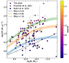 |
Fig. 3. Diagram of M* versus SFR of the sample studied, colour coded according to the spectroscopic redshift. The data from Lockman–SpReSO are represented by circles, PR21 data are represented by diamonds, and RU14 data are represented by squares. The dotted line represents the Murray et al. (2011) limit for producing winds in galaxies. The blue, red, and green solid lines and shaded areas are the Popesso et al. (2023) fit for the main sequence and its scatter of 0.09 dex calculated at the minimum, median, and maximum redshift of the sample, respectively. |
3. Inflow and outflow study
To determine whether our objects have inflows or outflows we need to know the velocity difference, if any, between the selected absorption lines and the velocity of the system. To do this, the redshift of the object and the centre of the lines are required. The redshift was retrieved from Gonzalez-Otero et al. (2023) (see the paper for details) and is given in Table 1. The properties of the Mg II and Fe II lines were derived for this paper by fitting the spectral lines (see the Sect. 3 for details).
As we have already seen, the Fe II and Mg II lines are useful for studying the galactic flows. Some studies have described the UV lines and their main properties in detail (Erb et al. 2012; Martin et al. 2012; Zhu et al. 2015, and references therein). As with UV lines, their analysis with ground-based telescopes is limited to objects with redshifts ≳0.4 owing to the attenuation of the UV component by the atmosphere; otherwise, it is necessarily to observe with space telescopes. Another major problem with these lines is the resonant emission that occurs in some of them, which fills in the absorption and makes it difficult to accurately measure the line. In Fig. 5 of Zhu et al. (2015) and their Appendix A are gathered the energy-level diagrams of the Fe II, Mg II, and Mg I atoms for the transitions that we studied for this paper. Lines that do not produce fluorescent emission (those that can only be de-excited to the ground state) are more affected by emission filling. When this happens, the line profile may be modified.
Absorption is produced by the gas between the observer and the galaxy while emission can come from other parts of the galaxy, leading to a difference between the centres of the absorption and emission components. Among the lines used in our study, the one most affected by this effect is the Fe IIλ2382 line, since the only way to de-excite it is by resonant emission. In addition, the Fe IIλ2344 line produces a fluorescent emission at 2381.49 Å, which also affects the Fe IIλ2382 line. Even the Fe IIλ2600 line could suffer from emission filling as the fluorescent emission it produces at 2626 Å has a very low probability of occurring. Lines such as Fe IIλ2373 and Fe IIλ2586 suffer very little from this effect because the fluorescent emission de-excitation channels have high probabilities of occurrence (high Einstein A coefficient), so the lines suffer very little from emission filling.
However, when analysing the spectral lines of our sample, we found no emission filling effect. Figure 4 shows examples where both Fe II and Mg II lines are detected with no apparent emission filling effect. This was also seen in analyses of nearby galaxies, where the Na Iλλ 5890,96 lines showed little emission filling (Heckman et al. 2000; Martin 2005, 2006; Chen et al. 2010). This has been attributed to the presence of regions of high gas density and high neutral sodium concentration where the long path length of the scattered photons leads to a high probability of absorption by dust. The Lockman–SpReSO survey objects are selected for their IR emission, in other words they are dusty, as indicated by a mean extinction of AV ∼ 2.7 mag. Furthermore, as we have discussed previously (see Table 1), we see that most of the objects are LIRGs or even ULIRGs, which favours the non-production of emission filling according to the above reasoning. In the work of Prochaska et al. (2011), they find that the Fe II fluorescence lines scale with the amount of emission filling. As they are not detected in the spectra of our sample, this supports the fact that no emission filling effect is found in the spectral lines.
 |
Fig. 4. Example fit for the doublets studied in this study for source 77155. On the left is the Mg IIλλ2796, 2803 fit with the residuals at the bottom. The Mg Iλ2852 line is also visible in this slice of the spectrum. In the centre, the fit for Fe IIλλ2586, 2600, also with the residuals of the fit at the bottom. On the right, using the same schedule, the case of Fe IIλλ2374, 82 with a low S/N ratio. You can also see the C II] λ2325 in emission and Fe IIλ2344 in absorption. |
3.1. Fitting of absorption lines
The lines were measured using the same procedure as that used by Gonzalez-Otero et al. (2023) where the Python package LMFIT4 (Newville et al. 2014) was used for the measurement of the most intense spectral lines. LMFIT allows us to perform a non-linear least-squares minimisation line fitting routine with the desired model. The lines were fitted using a Gaussian model for the absorption component and a linear zero-slope continuum model. As we have seen, in the work of Rubin et al. (2014) and others (Chen et al. 2010; Xu et al. 2022, for example), each line is also fitted with a two component model: one fixed zero velocity component representing the ISM of the galactic region and a variable velocity component representing the galactic flow. However, the resolution of our study does not allow this type of component decomposition. The normalisation of the spectra was performed only in the analysis windows of each line or doublet line. The flat continuum model obtained in the fitting was used to normalise by the continuum.
Mg IIλλ2796, 2803, Fe IIλλ2374, 82, and Fe IIλλ2586, 2600 are doublets of spectral lines whose components are very close in wavelength. This implies that at the dispersion used (∼3–4 Å pix−1), depending also on the redshift, these doublets can appear blended. Therefore, in the case of these doublets, we fitted the two lines together with the continuum at the same time, that is two Gaussian components (one for each line) plus a linear model. In order to reduce the computational time, we have used the known relations of the lines as initial parameters of the models, but allowed them to fluctuate. As each doublet line is produced in the same region and under the same conditions in the galaxy, in the absence of emission filling or other phenomena, the width should be the same, that is, the same initial sigma value for the two Gaussian components. The same reasoning applies to the central wavelength of the line, where the length between peaks is known, although it is a free parameter in the fit. None of the fit parameters were fixed, so they were all allowed to vary during the fitting process. Finally, as the redshift is known, the spectra were transferred to rest-frame to measure the lines.
Figure 4 shows an example of the line fit for ID 77155. The different degrees of blending found in this particular source are representative for our sample. Each panel shows the fit of one of the doublets studied in this paper. Upper panels represent the fit performed and lower panels represent the residuals of the fit itself. The fit results of Mg IIλλ2796, 2803, Fe IIλλ2586, 2600 and Fe IIλλ2374, 82 (with the lowest S/N ratio) are shown from left to right.
In addition, from the line-fitting procedure we determined the rest-frame equivalent width (EW) of the lines to be analysed in relation to the physical properties of the galaxies. The values obtained and its errors are collected in Table 2. The error in the EW was calculated by propagating the error obtained for the Gaussian component and the continuum of each line when the EW was calculated (both errors were calculated in the line fitting process). As can be seen, the values of the EW are biased towards higher values, mainly due to the resolution of the Lockman–SpReSO spectra.
Rest-frame EW of the absorption lines measured for the objects from the Lockman–SpReSO catalogue.
Finally, using the centre of the Gaussian components obtained in the fit, we determined the velocity of the lines and hence the velocity difference between the material wind and the system. The errors in velocity have been propagated from the central wavelength error obtained in the fit of each line. In Table 3 we list the velocities obtained and its errors for the lines analysed.
Absorption line velocities measured for the objects from the Lockman–SpReSO catalogue.
4. Galactic flows properties analysis
4.1. Equivalent width analysis
There are studies in the literature that has led to claims of correlations between EW and certain galaxy properties. RU14 found that the EW of the absorption of Mg II is correlated with M* with a significance of 3.2σ under a parameter of the Spearman’s rank correlation coefficient5 (ρs) of ρs = 0.44 and with the SFR at a significance of 3.5σ (ρs = 0.48). For the EW of Fe II they found a correlation with SFR at a significance of 2.4σ (ρs = 0.46) while for M* they found no correlation, claiming that this may be because of the small M* range of their sample. PR21 performed a similar analysis with other data and found a similar correlation between the EW of Mg IIλ2796 (ρs = 0.67 at 3.2σ) and Fe II (ρs = 0.65 at 2.9σ) with the SFR. However, they found no significant correlation between EW and M*.
As we have seen, our objects are dusty and the effect of emission filling is not very important. Nevertheless, we focus our analysis on the Mg IIλ2796, the blue line of the doublet, which is less affected by this phenomenon. In Fig. 5, from left to right, we have plotted the EW of the Mg IIλ2796 line against M*, SFR, and specific SFR (sSFR) for the objects together from the Lockman–SpReSO, PR21 and RU14 samples. It can be seen that the Lockman–SpReSO galaxies populate regions of the plots that the Rubin and Prusinski objects barely do. The Lockman objects have larger EWs than the other samples, while the properties of the galaxies are comparable (see Fig. 2). The EW of the Lockman objects is biased towards higher values due to the low resolution of the observations, with values close to 10 Å and minimum values around 2 Å. However, this allows us to sample other regions of the parameter space and to study in more detail how the galaxy properties relate to the EW of the lines.
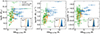 |
Fig. 5. Plot of the Mg IIλ2796 EW versus M*, SFR, and sSFR (from left to right). The empty blue circles are the results obtained here, the empty orange diamonds are the results of PR21 and the green empty squares are the results of RU14. The inset graph in each panel contains the probability distribution of the Spearman parameter from the bootstrap procedure in blue (see the text for more details) and the expected distribution in the uncorrelated case is shown in orange. The value of the mode of the obtained distribution and the significance in sigmas for the obtained correlation are also included. See the Sect. 4.1 for a discussion of correlation. |
To test whether there is a correlation between the EW and the properties of the galaxies, Spearman tests were performed by grouping the three data sets. To estimate the confidence intervals of the correlation, the bootstrap method was applied 107 times. The blue histograms in the inset of each panel of Fig. 5 represent the probability distribution function (PDF) of the Spearman parameter obtained in the bootstrap simulations and the dashed lines mark the mode of the PDF. The expected distribution for the case where there is no correlation between the variables6 is plotted in orange and the mode of Spearman parameter distribution and the significance are typed. It can be seen that for M* the data suggest a positive correlation with the EW, a mode of ρs = 0.43 being obtained at a significance of 4.5σ, indicating that the greater the mass of the object, the greater the capacity to generate material winds. This result differs from that obtained in the framework of PR21, but confirms that found by RU14, mainly owing to the joint study of all the data, which adds more statistics to the entire range of values, both EW and M*. A positive correlation was also found when examining the SFR with a mode of ρs = 0.42 at a significance of 4.4σ. As we have already discussed, Lockman data add more statistic significance in the high SFR area of the graph, thus better defining the behaviour in this area. The correlation found is not as strong as the one discovered in the work of PR21 and RU14, but the significance is higher owing to the larger data set. In the case of sSFR, no correlation was found with the EW of Mg II. The distribution obtained from the bootstrap simulations and that expected in the case of non-correlation are very close with a mode of ρs = 0.11 at a significance of 1.1σ.
In Fig. 6 we plot the EW of Fe IIλ2586 with respect to the properties of the galaxies in our study, together with the RU14 data, using the same procedure and symbols as in Fig. 5. It is observed that the EW correlates with M* in a similar way to that found for Mg II, with ρs = 0.43 at 3.3σ of significance. This result differs from that of RU14, who found no correlation between the parameters (ρs = 0.07 at 0.4σ). The significant difference in the EW between the data from RU14 and Lockman–SpReSO, mainly due to the different nature of the objects according to the selection criteria, coupled with the increase in the statistics, means that we can further populate the diagram and recover the correlation found between the EW of Mg II and M*. The correlation between the SFR and the EW of Fe II is the strongest found in this study, with a positive correlation where a mode of ρs = 0.69 was found in the bootstrap simulations at 5.3σ of significance. Once more, galaxies with higher SFRs can produce stronger winds. For the sSFR, there is still no significant correlation with the EW (ρs = 0.33 at 2.5σ).
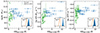 |
Fig. 6. Plot of the Fe IIλ2586 EW versus M*, SFR, and sSFR (from left to right). The empty blue circles are the results of this paper and the empty green squares are the results of RU14. The inset plots represent the same idea as in Fig. 5. See the Sect. 4.1 for a discussion of correlation. |
PR21 carried out the study of the Fe II lines using an EW-weighted average because they found the Fe II lines to be saturated in their spectra. In order to compare our data with their results, we calculated an EW-weighted average of the Fe II lines present in our objects and we show the results found in Fig. 7. The correlation with M* is very weak (ρs = 0.31) with a significance of 1.9σ. In this comparison, the bootstrap distribution and the expected distribution are wider than in the previous cases, mainly because of the smaller data set used. For the SFR we find a significant correlation (ρs = 0.62) at 3.9σ. This result is consistent with the results of PR21 and with the previous comparison with what RU14 found. This correlation supports the hypothesis that Fe II lines are more intense at higher SFRs of galaxies. The sSFR also shows a slight correlation (ρs = 0.52) at 3.2σ with the average EW, which we did not find in the previous comparisons. This relation may be due to the smaller statistics we have for log(sSFR) < −9.5, with only two sources in this region.
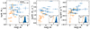 |
Fig. 7. Weighted EW average of the Fe II lines versus M*, SFR, and sSFR (from left to right). The empty blue circles are the results of this paper and the empty orange diamonds are the results of PR21. The inset plots represent the same idea as in Fig. 5. See the Sect. 4.1 for a discussion of correlation. |
4.2. Velocity analysis
As we show above, the spectral resolution of the Lockman–SpReSO spectra is not the commonly used resolution for the analysis of outflows. It can lead to large errors in the measurement of properties derived from spectral lines, such as the velocity of the ejected material, as can be seen from Table 3. Despite this severe limitation our sample increases the number of objects that can be studied in this still investigated topic. The initial results provide a fundamental basis for future research with higher resolution, which will help to reduce the margin of error and provide more accurate knowledge about the physical conditions of our sample. Using the velocities obtained we have estimated which objects are receiving an inflow of material, which are ejecting material from the galaxy star-forming regions, and which have velocities compatible with zero (no wind).
Following the criteria used for the EW analysis, we studied the Fe IIλ2586 and Mg IIλ2796 lines to distinguish between galaxies with outflows, inflows, and gas at the systemic velocity. Analysing the Fe IIλ2586 line, of the 18 objects retrieved from Lockman–SpReSO, nine show material outflows, five show material inflows, and four show velocities compatible with zero, namely absorption only. In the analysis of the Mg IIλ2796 line, ten objects show outflows, one shows an inflow, and seven have velocities compatible with zero. Considering the three objects classified as AGN, two (120237 and 206641) show an outflows in the Fe IIλ2586 line and object 206679 has velocities compatible with zero. The Mg IIλ2796 line is available only in pure absorption for the object 206679, and has an outflow-compatible velocity. The discrepancy between the Fe II and Mg II results can be attributed to the high degree of blending of the Mg II doublet lines with respect to the Fe II doublet lines, mainly because of the small wavelength separation between the centres of the Mg II lines (∼ 7 Å) and the resolution at which they are observed in Lockman–SpReSO. Furthermore, object 206679, at redshift ∼1.44, could be a Fe II low-ionisation broad absorption-line quasar (FeLoBALQ) candidate that shows an AGN-type nature by the presence of C III] emission, also noticed by Schmidt et al. (1998), and might be an example of a loitering outflow representing a new class of FeLoBALQs described by Choi et al. (2022). The peculiarity of these FeLoBALQs is that they have low flow velocities and high column density winds located at log(Rd) ≲ 1 pc where Rd is the distance to the centre.
In Fig. 8 we plot the Mg IIλ2796 velocities using the data from Lockman–SpReSO, PR21, and RU14 against the physical parameters of the galaxies, where the possible existence of a correlation is analysed in the same way as the EW (see Sect. 4.1). To investigate the correlation between outflow velocity and galaxy properties, we restrict the sample to objects that satisfy δv < 50 km s−1, excluding inflows from the study while accounting for measurement errors. The result is that the Mg IIλ2796 velocity is not correlated with M*, SFR, or sSFR as the distributions obtained from the bootstrap simulations are similar to those expected in the uncorrelated case. The same analysis is carried out for the Fe IIλ2586 line using the RU14 and Lockman data and is shown in Fig. 9. Examining the distributions of the bootstrap simulations, we find that there is no significant correlation between the Fe IIλ2586 velocity and the M*. However, there is a negative correlation between velocity and SFR with ρ = −0.34 at 3.6σ of significance. The study on sSFR shows a weaker negative correlation (ρ = −0.27) at 2.9σ.
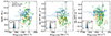 |
Fig. 8. Mg IIλ2796 velocity versus M*, SFR, and sSFR (from left to right). The symbols and colour coding are the same as for Fig. 5. See Sect. 4.2 for a discussion of correlation analysis. |
If we examine the mean velocity of all Fe II lines weighted by the error, we can use the PR21 and Lockman–SpReSO data in conjunction. As can be seen in Fig. 10, there is a strong correlation of the velocity with the M* (ρ = −0.43) and SFR (ρ = −0.57). The significance identified is lower due to the limited statistics available in this case and the narrow range of values that can be studied for the parameters. These results differ from that obtained in the framework of PR21, where no correlations were found with a significance greater than 1.4σ. They argue that the lack of correlation is due to the short range of SFR in their objects, which, when combined with the intrinsic scatter of the relationship between SFR and velocity, makes it difficult to find a correlation. Additionally, the study may be affected by a systemic component of the ISM that scales with the SFR, as expected from the Schmidt-Kennicut law (Kennicutt & Evans 2012). This component may have a greater impact on studies that use a single component fit of the spectral lines.
In contrast of our results, Rupke et al. (2005b) studying 78 starburst-dominated LIRGs and analysing the Na I absorption, found that the outflow velocity and properties of these galaxies are independent. However, Martin (2005), analysing 18 ULIRGs, found that the Na I velocity follows a relation Δv ∼ SFR0.35. Weiner et al. (2009), studying a coadded spectra of 1406 galaxies at z ∼ 2 from the DEEP2 redshift survey, also found that Mg II absorption in outflows is stronger and reaches higher velocities for more massive galaxies; they obtained a similar relationship for the velocity Δv ∼ SFR0.3. Heckman et al. (2015), studying the UV absorption lines of 39 low-redshift starburst galaxies, found that there is a strong correlation of the velocity they measured with the SFR and SFR surface density (ΣSFR), but a weak correlation with M*. This result is supported by Chisholm et al. (2015), who analysed the Si II absorption lines in 48 nearby SFGs. They found a correlation with a significance of 3–3.5σ between the outflow velocity and galaxy properties such as SFR and M*. Davis et al. (2023) created a sample with a wide range in M* and SFR. They studied 46 late-stage galaxy mergers in conjunction with data from ten other papers about outflow winds and discovered a significant correlation between outflow velocities and SFR.
As can be seen, our results are inn good agreement with those found in other studies. The Lockman-SpReSO data is crucial for this study. Figures 8–10 demonstrate that the FIR-selected galaxies occupy regions in the charts where there were previously few objects, particularly in the higher SFR regions. This provides a more comprehensive sampling of the parameter space, allowing for a more detailed analysis of the general properties of galactic flows. In addition to higher SFRs, the velocities of the Fe II line tend to be higher than those of PR21 and RU14 sample (Figs. 9 and 10), increasing the available range of velocities in the correlation study.
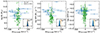 |
Fig. 9. Fe IIλ2586 velocity versus M*, SFR, and sSFR (from left to right). The symbols and colours are as in Fig. 5. See Sect. 4.2 for a discussion of correlation. |
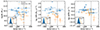 |
Fig. 10. Average Fe II velocity versus M*, SFR, and sSFR (from left to right). The symbols and colours are as in Fig. 5. See the Sect. 4.2 for a discussion of correlation. |
4.3. Local covering factor and optical depth
The observed depth of an absorption line depends on the optical depth (τ) of an absorbing cloud, and also on the fraction of the background source which the cloud covers, C. For a continuum-normalised spectrum, the residual intensity I of the absorption feature is given by
If two absorption lines are observed closely in wavelength, for example two components of a multiplet of the same ion, for which the ratio of the optical depth is known (α), we can solve for C and τ. The ratio of optical depths is the ratio of the oscillator strengths f of the lines which can be found, for example, in Morton (2003) and references therein. If fb = αfr then τb = ατr, and the residual intensities in the red and blue components of the line are:
and
These equations must be solved numerically. See a more detailed discussion in Benn et al. (2005).
In our case, we observe the pairs of absorption lines Mg IIλλ2796, 2803, Fe IIλλ2374, 82, and Fe IIλλ2586, 2600. By measuring the residual intensities and knowing the oscillator strengths, we then estimate the covering factors (C), optical depths (τ0) and ionic column densities (N). As our spectral resolution is not high enough, covering factors should be taken as lower limits.. Results are shown in Table 4 where we show only the results for the Fe II absorption lines, because in most cases blending of the Mg II doublet makes it impossible to obtain a physical solution or is unreliable. In some cases it is also very difficult even for Fe II lines.
Covering factor, optical depth, and ionic column density obtained in the analysis of the Fe II doublet lines.
From the above we have estimated ion column densities (see Table 4). Our data, limited by low spectral resolution and the lack of other ionised species, do not allow us to constrain ionisation parameters or electron densities. We can, however, crudely estimate hydrogen column densities by assuming solar metallicity, no depletion of Fe, and 100% of ionisation for the singly ionised iron (Eq. (13) in Martin et al. 2012). For our outflows, H I column densities are estimated to be in the range log(N(H) I)) ∼ 19.7–20.5 cm−2, and in some cases can be up to log(N(H) I)) = 21. These large values seem unlikely, so we would expect higher than solar metallicities. Alternatively, for a control test, we can estimate H I column densities using the relationship defined in Ménard & Chelouche (2009) between H I column densities and rest frame Mg II EW. We measured Mg II EWs to be on average ∼ 5 Å, giving log(N(H) I)) ∼ 20.7 cm−2, consistent with our previous estimate.
Ionic densities and covering factors are similar to those in the literature (Martin et al. 2012). Also, average densities are log(N) ≲ 16 cm−2 so that we could conclude that we observed similar galactic outflows as in previous studies; that is, typical mass flux in the low-ionisation outflows can be of the order of ∼23 M⊙ yr−1 (Eq. (12) from Martin et al. 2012).
5. Summary and conclusions
In this paper, we present a study of the galactic flows in objects from the Lockman–SpReSO project (Gonzalez-Otero et al. 2023). The objects were selected for having Fe II lines in absorption, and Mg II lines in absorption and emission. We find 21 objects with redshift in the range 0.5 ≲ z ≲ 1.45, of which three are classified as AGN (González-Otero, in prep.). The objects in the sample span an M* range of 9.89 < log(M*/M⊙) < 11.50 and are (U)LIRGs (10.84 < log(LTIR/L⊙) < 12.53) with relatively high log(SFR) between 1.01 and 2.70. We determined the systemic velocities of the objects and measured the EW and velocities of the Fe IIλλ2374, 82, Fe IIλλ2586, 2600, Fe IIλ2344, Mg IIλλ2796, 2803, and Mg Iλ2852 spectral lines.
The EWs and line velocities were used to explore possible correlations with the M*, SFR, and sSFR values of the galaxies. In order to obtain statistically significant results, we performed a joint analysis of our sample of 18 objects with an additional 22 and 105 galaxies from PR21 and RU14, respectively. Bootstrap simulations were performed on the Spearman rank test to check for the existence of correlations between the properties. The inclusion of Lockman–SpReSO objects, selected for their FIR emission, adds great value to the sample, because to the best of our knowledge there are very few such studies based on LIRGs in the literature (e.g. Banerji et al. 2011). This helps us to validate whether the results obtained with other types of objects are also valid for the FIR-selected objects.
Using the three samples as a whole, we find the EW of Mg IIλ2796 to correlate strongly, ρs = 0.43 (ρs = 0.42) and significantly at 4.5σ (4.4σ) with M* (SFR). This result is in good agreement with the findings of RU14, but is only in agreement with those of PR21 with respect to the SFR relationship; these latter authors found no correlation of EW with M*. The Lockman–SpReSO sample enables a more in-depth examination of the correlations between EW and galaxy properties. The EWs of these objects occupy regions of the parameter space where object density is very low, with higher values than in the RU14 and PR21 samples. This enables us to expand the boundaries of the relationships. The Mg IIλ2796 line velocity has no correlation (ρs ∼ −0.1) with the properties of the galaxies in the sample. Davis et al. (2023) find a positive correlation between velocity and SFR for the Mg II line. The discrepancy observed could be attributed to the effect of emission-line infilling, which dilutes the lines and introduces errors. Table 5 contains a summary of the Spearman coefficient obtained in the analysis of the Mg IIλ2796 line.
Summary of the Spearman rank correlation coefficient and the significance found in the study of the Mg IIλ2796 line.
For the analysis of the Fe II lines, separate studies were carried out for the PR21 and RU14 samples. In the sample with Lockman–SpReSO and RU14 data, a positive correlation ρs = 0.43 (ρs = 0.69) and a significant one at 3.3σ (5.3σ) were found with the M* (SFR) and the EW of Fe IIλ2586. With the sSFR, the correlation found is not very strong (ρs = 0.33) and of marginal significance (2.5σ). The velocity has no significant correlation with M*, but a strong correlation (ρ = −0.34) with high significance (3.6σ) is found with SFR. This result implies that the velocity of Fe II spectral lines remains decoupled from M* but not from SFR; in other words, the energy to which the material is exposed depends more on SFR than on M*. A summary of the correlations can be seen in Table 6. To study the Lockman–SpReSO and PR21 sample as a whole, we performed weighted averages of the EW and velocities of the Fe II lines measured in the Lockman–SpReSO objects. We find that EWavg is strongly correlated with the SFR (ρs = 0.62) at 3.9σ and more marginally correlated with the M* (ρs = 0.31) and sSFR (ρs = 0.52) at 1.9σ and 3.2σ, respectively. The average velocity also shows strong correlations with M* (ρ = −0.43) and SFR (ρ = −0.57). This is consistent with the results above that show that the velocity is dependent on the properties of the SFR. In general, thanks to the inclusion of the Lockman–SpReSO objects selected for their FIR emission – of which little is known compared to galactic flows in distant FIR objects –, we can confirm the results of previous studies and find discrepancies with others. A summary of the correlations obtained for the weighted average of Fe II lines is provided in Table 7.
Summary of the Spearman rank correlation coefficient and the significance found in the study of the Fe IIλ2586 line.
Summary of the Spearman rank correlation coefficient and the significance found in the study of the weighted average of the Fe II lines.
Although the spectral resolution and dispersion used in the Lockman–SpReSO observations (R ∼ 500, ∼4 Å pix−1) are not commonly used for outflow analysis, where higher resolutions are usually required, we were able to detect the existence of nine (ten) galactic outflows, five (one) inflows, and four (seven) absorption-only objects based on the velocities obtained for the Fe IIλ2586 (Mg IIλ2796) line. In addition, of the three objects classified as AGN, object 206679 was found to be a clear candidate ‘loitering outflow’, a new class of iron low-ionisation broad absorption (FeLoBAL) quasar characterised by low flow velocities (v ≲ 2000 kms−1) and high-column-density winds located at log(Rd) ≲ 1 pc.
Finally, it is important to highlight that this study was not initially planned, but rather emerged from the serendipitous discovery of these objects in the Lockman–SpReSO data. Despite the unplanned nature of the study, the findings provide valuable insights into the characteristics and behaviour of these objects. Higher-resolution observations will help us to better constrain and study the velocities of the objects with increased accuracy, and will provide more information about the FeLoBAL quasar candidate. However, this study undoubtedly sheds more light on the study of galactic flows by adding objects of a different nature compared to those studied so far, as they are objects selected for their FIR emission.
Spearman’s correlation coefficient is a statistical method used to measure the strength and direction of the relationship between two variables. It assesses if there is a consistent monotonic relationship between the ranks of the variables, without assuming a linear association. The correlation coefficient ranges from −1 to 1, with positive values indicating a direct relationship, negative values indicating an inverse relationship, and 0 indicating no monotonic relationship. The test provides a p-value to determine the statistical significance of the observed correlation. It is commonly used when dealing with non-linear or non-normally distributed data.
For large samples (n ≥ 30), the expected distribution of the Spearman parameter tends to be a normal one  .
.
Acknowledgments
We thank the anonymous referee for their useful report. This work was supported by the Evolution of Galaxies project, of references AYA2017-88007-C3-1-P, AYA2017-88007-C3-2-P, AYA2018-RTI-096188-BI00, PID2019-107408GB-C41, PID2019-106027GB-C41, PID2021-122544NB-C41, PID2021-122544NB-C43, PID2022-136598NB-C33, and MDM-2017-0737 (Unidad de Excelencia María de Maeztu, CAB), within the Programa estatal de fomento de la investigación científica y técnica de excelencia del Plan Estatal de Investigación Científica y Técnica y de Innovación (2013-2016) of the Spanish Ministry of Science and Innovation/State Agency of Research MCIN/AEI/ 10.13039/501100011033 and by ‘ERDF A way of making Europe’. This work is based on observations made with the Gran Telescopio Canarias (GTC) at Roque de los Muchachos Observatory on the island of La Palma, with the William Herschel Telescope (WHT) at Roque de los Muchachos Observatory on the island of La Palma and on observations at Kitt Peak National Observatory, NSF’s National Optical-Infrared Astronomy Research Laboratory (NOIRLab Prop. ID: 2018A-0056; PI: González-Serrano, J.I.), which is operated by the Association of Universities for Research in Astronomy (AURA) under a cooperative agreement with the National Science Foundation. This research has made use of the NASA/IPAC Extragalactic Database (NED), which is funded by the National Aeronautics and Space Administration and operated by the California Institute of Technology. E.B. and I.C.G. acknowledge support from DGAPA-UNAM grant IN119123. J.N. acknowledges the support of the National Science Centre, Poland through the SONATA BIS grant 2018/30/E/ST9/00208 Y.K. acknowledges support from DGAPA-PAPIIT grant IN102023. The authors thank Terry Mahoney (at the IAC’s Scientific Editorial Service) for his substantial improvements of the manuscript.
References
- Baldwin, J. A., Phillips, M. M., & Terlevich, R. 1981, PASP, 93, 5 [Google Scholar]
- Banerji, M., Chapman, S. C., Smail, I., et al. 2011, MNRAS, 418, 1071 [NASA ADS] [CrossRef] [Google Scholar]
- Benn, C. R., Carballo, R., Holt, J., et al. 2005, MNRAS, 360, 1455 [NASA ADS] [CrossRef] [Google Scholar]
- Boquien, M., Burgarella, D., Roehlly, Y., et al. 2019, A&A, 622, A103 [NASA ADS] [CrossRef] [EDP Sciences] [Google Scholar]
- Burgarella, D., Buat, V., & Iglesias-Páramo, J. 2005, MNRAS, 360, 1413 [NASA ADS] [CrossRef] [Google Scholar]
- Calzetti, D., Armus, L., Bohlin, R. C., et al. 2000, ApJ, 533, 682 [NASA ADS] [CrossRef] [Google Scholar]
- Cepa, J., Aguiar, M., Escalera, V. G., et al. 2000, Proc. SPIE, 4008, 623 [NASA ADS] [CrossRef] [Google Scholar]
- Chabrier, G. 2003, PASP, 115, 763 [Google Scholar]
- Chen, Y.-M., Tremonti, C. A., Heckman, T. M., et al. 2010, AJ, 140, 445 [Google Scholar]
- Chisholm, J., Tremonti, C. A., Leitherer, C., et al. 2015, ApJ, 811, 149 [NASA ADS] [CrossRef] [Google Scholar]
- Choi, H., Leighly, K. M., Terndrup, D. M., et al. 2022, ApJ, 937, 74 [NASA ADS] [CrossRef] [Google Scholar]
- Cid Fernandes, R., Stasińska, G., Mateus, A., & Vale Asari, N. 2011, MNRAS, 413, 1687 [Google Scholar]
- Cooksey, K. L., Prochaska, J. X., Chen, H.-W., Mulchaey, J. S., & Weiner, B. J. 2008, ApJ, 676, 262 [NASA ADS] [CrossRef] [Google Scholar]
- Davis, J. D., Tremonti, C. A., Swiggum, C. N., et al. 2023, ApJ, 951, 105 [NASA ADS] [CrossRef] [Google Scholar]
- Domínquez Palmero, L., Cano, D., Fariña, C., et al. 2014, SPIE Conf. Ser., 9147, 914778 [Google Scholar]
- Donley, J. L., Koekemoer, A. M., Brusa, M., et al. 2012, ApJ, 748, 142 [Google Scholar]
- Erb, D. K., Quider, A. M., Henry, A. L., & Martin, C. L. 2012, ApJ, 759, 26 [CrossRef] [Google Scholar]
- Finley, H., Bouché, N., Contini, T., et al. 2017a, A&A, 605, A118 [NASA ADS] [CrossRef] [EDP Sciences] [Google Scholar]
- Finley, H., Bouché, N., Contini, T., et al. 2017b, A&A, 608, A7 [NASA ADS] [CrossRef] [EDP Sciences] [Google Scholar]
- Gonzalez-Otero, M., Padilla-Torres, C. P., Cepa, J., et al. 2023, A&A, 669, A85 [NASA ADS] [CrossRef] [EDP Sciences] [Google Scholar]
- Heckman, T. M., Lehnert, M. D., Strickland, D. K., & Armus, L. 2000, ApJS, 129, 493 [Google Scholar]
- Heckman, T. M., Alexandroff, R. M., Borthakur, S., Overzier, R., & Leitherer, C. 2015, ApJ, 809, 147 [Google Scholar]
- Jones, T., Stark, D. P., & Ellis, R. S. 2012, ApJ, 751, 51 [Google Scholar]
- Kennicutt, R. C., Jr 1998, ARA&A, 36, 189 [NASA ADS] [CrossRef] [Google Scholar]
- Kennicutt, R. C., & Evans, N. J. 2012, ARA&A, 50, 531 [NASA ADS] [CrossRef] [Google Scholar]
- Kobulnicky, H. A., & Kewley, L. J. 2004, ApJ, 617, 240 [CrossRef] [Google Scholar]
- Leclercq, F., Bacon, R., Verhamme, A., et al. 2020, A&A, 635, A82 [NASA ADS] [CrossRef] [EDP Sciences] [Google Scholar]
- Luo, B., Brandt, W. N., Xue, Y. Q., et al. 2017, ApJS, 228, 2 [Google Scholar]
- Martin, C. L. 2005, ApJ, 621, 227 [NASA ADS] [CrossRef] [Google Scholar]
- Martin, C. L. 2006, ApJ, 647, 222 [NASA ADS] [CrossRef] [Google Scholar]
- Martin, C. L., Shapley, A. E., Coil, A. L., et al. 2012, ApJ, 760, 127 [Google Scholar]
- Ménard, B., & Chelouche, D. 2009, MNRAS, 393, 808 [CrossRef] [Google Scholar]
- Messias, H., Afonso, J., Salvato, M., Mobasher, B., & Hopkins, A. M. 2012, ApJ, 754, 120 [Google Scholar]
- Morton, D. C. 2003, ApJS, 149, 205 [Google Scholar]
- Murray, N., Ménard, B., & Thompson, T. A. 2011, ApJ, 735, 66 [NASA ADS] [CrossRef] [Google Scholar]
- Newville, M., Stensitzki, T., Allen, D. B., & Ingargiola, A. 2014, https://doi.org/10.5281/zenodo.11813 [Google Scholar]
- Oke, J. B., & Gunn, J. E. 1983, ApJ, 266, 713 [NASA ADS] [CrossRef] [Google Scholar]
- Péroux, C., & Howk, J. C. 2020, ARA&A, 58, 363 [CrossRef] [Google Scholar]
- Pettini, M., & Pagel, B. E. J. 2004, MNRAS, 348, L59 [NASA ADS] [CrossRef] [Google Scholar]
- Pilyugin, L. S., & Grebel, E. K. 2016, MNRAS, 457, 3678 [NASA ADS] [CrossRef] [Google Scholar]
- Popesso, P., Concas, A., Cresci, G., et al. 2023, MNRAS, 519, 1526 [Google Scholar]
- Prochaska, J. X., Kasen, D., & Rubin, K. 2011, ApJ, 734, 24 [Google Scholar]
- Prusinski, N. Z., Erb, D. K., & Martin, C. L. 2021, AJ, 161, 212 [NASA ADS] [CrossRef] [Google Scholar]
- Rubin, K. H. R., Weiner, B. J., Koo, D. C., et al. 2010, ApJ, 719, 1503 [NASA ADS] [CrossRef] [Google Scholar]
- Rubin, K. H. R., Prochaska, J. X., Koo, D. C., et al. 2014, ApJ, 794, 156 [Google Scholar]
- Rupke, D. S., Veilleux, S., & Sanders, D. B. 2005a, ApJ, 632, 751 [NASA ADS] [CrossRef] [Google Scholar]
- Rupke, D. S., Veilleux, S., & Sanders, D. B. 2005b, ApJS, 160, 115 [Google Scholar]
- Schmidt, M., Hasinger, G., Gunn, J., et al. 1998, A&A, 329, 495 [NASA ADS] [Google Scholar]
- Shapley, A. E., Steidel, C. C., Pettini, M., & Adelberger, K. L. 2003, ApJ, 588, 65 [Google Scholar]
- Skelton, R. E., Whitaker, K. E., Momcheva, I. G., et al. 2014, ApJS, 214, 24 [Google Scholar]
- Steidel, C. C., Erb, D. K., Shapley, A. E., et al. 2010, ApJ, 717, 289 [Google Scholar]
- Szokoly, G. P., Bergeron, J., Hasinger, G., et al. 2004, ApJS, 155, 271 [NASA ADS] [CrossRef] [Google Scholar]
- Tremonti, C. A., Heckman, T. M., Kauffmann, G., et al. 2004, ApJ, 613, 898 [Google Scholar]
- Tumlinson, J., Peeples, M. S., & Werk, J. K. 2017, ARA&A, 55, 389 [Google Scholar]
- Veilleux, S., Cecil, G., & Bland-Hawthorn, J. 2005, ARA&A, 43, 769 [NASA ADS] [CrossRef] [Google Scholar]
- Veilleux, S., Maiolino, R., Bolatto, A. D., & Aalto, S. 2020, A&A Rev., 28, 2 [NASA ADS] [CrossRef] [Google Scholar]
- Weiner, B. J., Coil, A. L., Prochaska, J. X., et al. 2009, ApJ, 692, 187 [Google Scholar]
- Xu, X., Heckman, T., Henry, A., et al. 2022, ApJ, 933, 222 [NASA ADS] [CrossRef] [Google Scholar]
- Zhu, G. B., Comparat, J., Kneib, J.-P., et al. 2015, ApJ, 815, 48 [NASA ADS] [CrossRef] [Google Scholar]
Appendix A: Cutouts and SED fits of the Lockman–SpReSO objects
 |
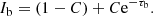
Fig. A.1. Cutouts (top left), SED fits (top right), and spectra slices (bottom) for the object ID 123207 studied in this paper. The cutouts are made on the GTC image of the Lockman-SpReSO survey field (see Gonzalez-Otero et al. 2023 for details). The green dot represents the optical coordinates of the object. The blue circle marks nearby objects in the Lockman-SpReSO catalogue. The red rectangle represents the position and size of the slit used to observe the object. There are two types of slit: a small slit of 3 arcsec and a large slit of 10 arcsec (see Gonzalez-Otero et al. 2023 for more details). The red circle represents the position of the fibre. In the SED fits the best model is plotted as a solid black line, the photometric information of the object is plotted as empty violet circles, and the red filled circles are the fluxes obtained by the best model. The individual contributions of the models used are also plotted where the yellow line represents the attenuated stellar component, the blue dashed line is the unattenuated stellar component, the green line illustrates the nebular emission, and the red line is the dust emission. The relative residuals of the flux for the best model are plotted at the bottom. The spectral slices show the absorption lines studied in this paper. The spectra have been normalised to the continuum. The grey vertical dashed lines represent the rest-frame wavelength of the lines. |
 |
Fig. A.10. Same as Fig. A.1 but for object ID 120257. |
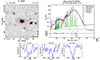 |
Fig. A.11. Same as Fig. A.1 but for object ID 95958. |
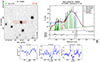 |
Fig. A.12. Same as Fig. A.1 but for object ID 116662. |
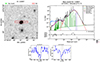 |
Fig. A.13. Same as Fig. A.1 but for object ID 133957. |
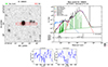 |
Fig. A.14. Same as Fig. A.1 but for object ID 186820. |
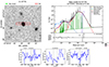 |
Fig. A.15. Same as Fig. A.1 but for object ID 97778. |
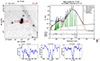 |
Fig. A.16. Same as Fig. A.1 but for object ID 77155. |
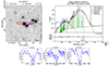 |
Fig. A.17. Same as Fig. A.1 but for object ID 102473. |
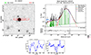 |
Fig. A.18. Same as Fig. A.1 but for object ID 120237. |
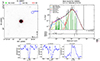 |
Fig. A.19. Same as Fig. A.1 but for object ID 206641. |
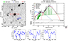 |
Fig. A.20. Same as Fig. A.1 but for object ID 78911. |
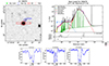 |
Fig. A.21. Same as Fig. A.1 but for object ID 206679. |
All Tables
Basic information on the objects selected from the Lockman–SpReSO catalogue, ordered by increasing redshift.
Rest-frame EW of the absorption lines measured for the objects from the Lockman–SpReSO catalogue.
Absorption line velocities measured for the objects from the Lockman–SpReSO catalogue.
Covering factor, optical depth, and ionic column density obtained in the analysis of the Fe II doublet lines.
Summary of the Spearman rank correlation coefficient and the significance found in the study of the Mg IIλ2796 line.
Summary of the Spearman rank correlation coefficient and the significance found in the study of the Fe IIλ2586 line.
Summary of the Spearman rank correlation coefficient and the significance found in the study of the weighted average of the Fe II lines.
All Figures
|
Fig. 1. SFR versus M* of the SFGs selected for this study (red) compared to the Lockman–SpReSO sample (grey). The galaxies exhibiting Mg II and Fe II absorption lines populate the region with the highest density of objects in the parent sample. |
| In the text | |
|
Fig. 2. Main properties of the studied objects. The blue bars represent the objects from Lockman–SpReSO survey, the orange bars represent the objects from PR21 and the green bars are the objects from RU14. The top left panel shows the M* of the objects, the top right shows the spectroscopic redshift, the bottom left shows the SFR and, the bottom right shows the sSFR. |
| In the text | |
|
Fig. 3. Diagram of M* versus SFR of the sample studied, colour coded according to the spectroscopic redshift. The data from Lockman–SpReSO are represented by circles, PR21 data are represented by diamonds, and RU14 data are represented by squares. The dotted line represents the Murray et al. (2011) limit for producing winds in galaxies. The blue, red, and green solid lines and shaded areas are the Popesso et al. (2023) fit for the main sequence and its scatter of 0.09 dex calculated at the minimum, median, and maximum redshift of the sample, respectively. |
| In the text | |
|
Fig. 4. Example fit for the doublets studied in this study for source 77155. On the left is the Mg IIλλ2796, 2803 fit with the residuals at the bottom. The Mg Iλ2852 line is also visible in this slice of the spectrum. In the centre, the fit for Fe IIλλ2586, 2600, also with the residuals of the fit at the bottom. On the right, using the same schedule, the case of Fe IIλλ2374, 82 with a low S/N ratio. You can also see the C II] λ2325 in emission and Fe IIλ2344 in absorption. |
| In the text | |
|
Fig. 5. Plot of the Mg IIλ2796 EW versus M*, SFR, and sSFR (from left to right). The empty blue circles are the results obtained here, the empty orange diamonds are the results of PR21 and the green empty squares are the results of RU14. The inset graph in each panel contains the probability distribution of the Spearman parameter from the bootstrap procedure in blue (see the text for more details) and the expected distribution in the uncorrelated case is shown in orange. The value of the mode of the obtained distribution and the significance in sigmas for the obtained correlation are also included. See the Sect. 4.1 for a discussion of correlation. |
| In the text | |
|
Fig. 6. Plot of the Fe IIλ2586 EW versus M*, SFR, and sSFR (from left to right). The empty blue circles are the results of this paper and the empty green squares are the results of RU14. The inset plots represent the same idea as in Fig. 5. See the Sect. 4.1 for a discussion of correlation. |
| In the text | |
|
Fig. 7. Weighted EW average of the Fe II lines versus M*, SFR, and sSFR (from left to right). The empty blue circles are the results of this paper and the empty orange diamonds are the results of PR21. The inset plots represent the same idea as in Fig. 5. See the Sect. 4.1 for a discussion of correlation. |
| In the text | |
|
Fig. 8. Mg IIλ2796 velocity versus M*, SFR, and sSFR (from left to right). The symbols and colour coding are the same as for Fig. 5. See Sect. 4.2 for a discussion of correlation analysis. |
| In the text | |
|
Fig. 9. Fe IIλ2586 velocity versus M*, SFR, and sSFR (from left to right). The symbols and colours are as in Fig. 5. See Sect. 4.2 for a discussion of correlation. |
| In the text | |
|
Fig. 10. Average Fe II velocity versus M*, SFR, and sSFR (from left to right). The symbols and colours are as in Fig. 5. See the Sect. 4.2 for a discussion of correlation. |
| In the text | |
|
Fig. A.1. Cutouts (top left), SED fits (top right), and spectra slices (bottom) for the object ID 123207 studied in this paper. The cutouts are made on the GTC image of the Lockman-SpReSO survey field (see Gonzalez-Otero et al. 2023 for details). The green dot represents the optical coordinates of the object. The blue circle marks nearby objects in the Lockman-SpReSO catalogue. The red rectangle represents the position and size of the slit used to observe the object. There are two types of slit: a small slit of 3 arcsec and a large slit of 10 arcsec (see Gonzalez-Otero et al. 2023 for more details). The red circle represents the position of the fibre. In the SED fits the best model is plotted as a solid black line, the photometric information of the object is plotted as empty violet circles, and the red filled circles are the fluxes obtained by the best model. The individual contributions of the models used are also plotted where the yellow line represents the attenuated stellar component, the blue dashed line is the unattenuated stellar component, the green line illustrates the nebular emission, and the red line is the dust emission. The relative residuals of the flux for the best model are plotted at the bottom. The spectral slices show the absorption lines studied in this paper. The spectra have been normalised to the continuum. The grey vertical dashed lines represent the rest-frame wavelength of the lines. |
| In the text | |
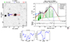 |
Fig. A.2. Same as Fig. A.1 but for object ID 96864. |
| In the text | |
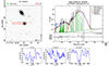 |
Fig. A.3. Same as Fig. A.1 but for object ID 101926. |
| In the text | |
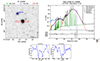 |
Fig. A.4. Same as Fig. A.1 but for object ID 120080. |
| In the text | |
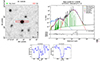 |
Fig. A.5. Same as Fig. A.1 but for object ID 118338. |
| In the text | |
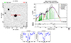 |
Fig. A.6. Same as Fig. A.1 but for object ID 95738. |
| In the text | |
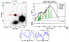 |
Fig. A.7. Same as Fig. A.1 but for object ID 109219. |
| In the text | |
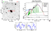 |
Fig. A.8. Same as Fig. A.1 but for object ID 94458. |
| In the text | |
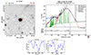 |
Fig. A.9. Same as Fig. A.1 but for object ID 92467. |
| In the text | |
|
Fig. A.10. Same as Fig. A.1 but for object ID 120257. |
| In the text | |
|
Fig. A.11. Same as Fig. A.1 but for object ID 95958. |
| In the text | |
|
Fig. A.12. Same as Fig. A.1 but for object ID 116662. |
| In the text | |
|
Fig. A.13. Same as Fig. A.1 but for object ID 133957. |
| In the text | |
|
Fig. A.14. Same as Fig. A.1 but for object ID 186820. |
| In the text | |
|
Fig. A.15. Same as Fig. A.1 but for object ID 97778. |
| In the text | |
|
Fig. A.16. Same as Fig. A.1 but for object ID 77155. |
| In the text | |
|
Fig. A.17. Same as Fig. A.1 but for object ID 102473. |
| In the text | |
|
Fig. A.18. Same as Fig. A.1 but for object ID 120237. |
| In the text | |
|
Fig. A.19. Same as Fig. A.1 but for object ID 206641. |
| In the text | |
|
Fig. A.20. Same as Fig. A.1 but for object ID 78911. |
| In the text | |
|
Fig. A.21. Same as Fig. A.1 but for object ID 206679. |
| In the text | |
Current usage metrics show cumulative count of Article Views (full-text article views including HTML views, PDF and ePub downloads, according to the available data) and Abstracts Views on Vision4Press platform.
Data correspond to usage on the plateform after 2015. The current usage metrics is available 48-96 hours after online publication and is updated daily on week days.
Initial download of the metrics may take a while.