| Issue |
A&A
Volume 617, September 2018
|
|
|---|---|---|
| Article Number | A62 | |
| Number of page(s) | 17 | |
| Section | Extragalactic astronomy | |
| DOI | https://doi.org/10.1051/0004-6361/201833281 | |
| Published online | 19 September 2018 | |
The MUSE Hubble Ultra Deep Field Survey
XII. Mg II emission and absorption in star-forming galaxies⋆
1
Université Lyon, Univ. Lyon1, ENS de Lyon, CNRS, Centre de Recherche Astrophysique de Lyon UMR5574, 69230, Saint-Genis-Laval, France
e-mail: This email address is being protected from spambots. You need JavaScript enabled to view it.
2
Institut de Recherche en Astrophysique et Planétologie (IRAP), Université de Toulouse, CNRS, UPS, 31400, Toulouse, France
3
Stockholm University, Department of Astronomy and Oskar Klein Centre for Cosmoparticle Physics, AlbaNova University Centre, 10691, Stockholm, Sweden
4
Leiden Observatory, Leiden University, PO Box 9513, 2300, RA Leiden, The Netherlands
5
Instituto de Astrofísica e Ciências do Espaço, Universidade do Porto, CAUP, Rua das Estrelas, 4150-762, Porto, Portugal
6
Sorbonne Universités, UPMC-CNRS, UMR7095, Institut d’Astrophysique de Paris, 75014, Paris, France
7
Department of Astronomy, University of Michigan, 1085 South University Ave, Ann Arbor, MI, 48109, USA
8
Department of Physics, ETH Zürich, Wolfgang-Pauli-Str. 27, 8093, Zürich, Switzerland
9
Leibniz-Institut für Astrophysik Potsdam (AIP), An der Sternwarte 16, 14482, Potsdam, Germany
10
Observatoire de Genève, Université de Genève, 51 Ch. des Maillettes, 1290, Versoix, Switzerland
Received:
23
April
2018
Accepted:
5
June
2018
Abstract
The physical origin of the near-ultraviolet Mg II emission remains an underexplored domain, unlike more typical emission lines that are detected in the spectra of star-forming galaxies. We explore the nebular and physical properties of a sample of 381 galaxies between 0.70 < z < 2.34 drawn from the MUSE Hubble Ultra Deep Survey. The spectra of these galaxies show a wide variety of profiles of the Mg II λλ2796, 2803 resonant doublet, from absorption to emission. We present a study on the main drivers for the detection of Mg II emission in galaxy spectra. By exploiting photoionization models, we verified that the emission-line ratios observed in galaxies with Mg II in emission are consistent with nebular emission from HII regions. From a simultaneous analysis of MUSE spectra and ancillary Hubble Space Telescope information through spectral energy distribution fitting, we find that galaxies with Mg II in emission have lower stellar masses, smaller sizes, bluer spectral slopes, and lower optical depth than those with absorption. This leads us to suggest that Mg II emission is a potential tracer of physical conditions that are not merely related to those of the ionized gas. We show that these differences in Mg II emission and absorption can be explained in terms of a higher dust and neutral gas content in the interstellar medium (ISM) of galaxies showing Mg II in absorption, which confirms the extreme sensitivity of Mg II to the presence of the neutral ISM. We conclude with an analogy between the Mg II doublet and the Ly α line that lies in their resonant nature. Further investigations with current and future facilities, including the James Webb Space Telescope, are promising because the detection of Mg II emission and its potential connection with Lyα could provide new insights into the ISM content in the early Universe.
Key words: galaxies: evolution / galaxies: ISM / ISM: lines and bands / ultraviolet: galaxies / ultraviolet: ISM
Based on observations made with ESO telescopes at the La Silla Paranal Observatory under programs 094.A-0289(B), 095.A-0010(A), 096.A-0045(A) and 096.A-0045(B).
© ESO 2018
 Open Access article, published by EDP Sciences, under the terms of the Creative Commons Attribution License (http://creativecommons.org/licenses/by/4.0), which permits unrestricted use, distribution, and reproduction in any medium, provided the original work is properly cited.
1. Introduction
Interpreting the physical nature of the spectral features observed in galaxy spectra is a non-trivial path to understand the physical processes at work within galaxies, and thereby, the galaxy population evolution through cosmic time. While optical lines have been extensively studied, ultraviolet (UV) lines have recently been under scrutiny (see Stark 2016 for an exhaustive review). The most explored line is the Lyman-α λ1215.67 (hereafter Lyα) line, along with the [C III]λ1907+C III]λ1909 (hereafter C III]) emission doublet, which is detected in the redshifted spectra of distant galaxies (e.g., Stark et al. 2015a; Maseda et al. 2017; Nakajima et al. 2018b). In addition, the complex profiles of combined stellar and nebular C IVλλ1548; 1551 and He IIλ1640 emissions are observed in the spectra of local metal-poor galaxies (e.g., Berg et al. 2016; Senchyna et al. 2017) and gravitationally lensed galaxies at higher redshift (e.g., Stark et al. 2015b; Vanzella et al. 2016; Mainali et al. 2017; Berg et al. 2018, and references therein).
The near-UV Mg II λλ2796, 2803 resonant doublet (hereafter Mg II) has been detected (in emission and/or absorption) in planetary nebulae and galaxy spectra. Intriguing, early works on planetary nebulae found the Mg II doublet to be absent, despite the presence of fainter magnesium emission lines, such as Mg Iλ4572, Mg Iλ4562, Mg Iλ4481, and Mg IIλ4391 in the same spectra. This led to the conclusion that Mg II might be an extremely sensitive tracer of some specific physical conditions of the gaseous nebulae themselves (Gurzadyan 1997).
The first detection of Mg II emission in a starbursting galaxy comes from the International Ultraviolet Explorer (IUE) spectrum of Tol1924-416 (Kinney et al. 1993). In the past decade, the redshifted Mg II emission has been detected in several studies of galactic winds (Weiner et al. 2009; Rubin et al. 2010, 2011; Giavalisco et al. 2011; Martin et al. 2012; Erb et al. 2012; Kornei et al. 2013; Finley et al. 2017b) and in the spectra of gravitationally lensed galaxies (Rigby et al. 2014; Karman et al. 2016; Bordoloi et al. 2016). This feature is often accompanied by blueshifted absorption, yielding a profile similar to a P-Cygni feature. Several explanations have been proposed for the origin of the Mg II emission, including the presence of an active galactic nucleus (AGN; Weiner et al. 2009) and resonant scattering in expanding winds (Rubin et al. 2010; Erb et al. 2012).
Erb et al. (2012) studied large-scale outflows in a sample of 96 star-forming galaxies at 1 ≲ z ≲ 2 with the Mg II doublet ranging from emission to absorption. They found Mg II emission to be more common at lower stellar masses and in galaxies with bluer UV slopes. Kornei et al. (2013) detected Mg II emission in ∼15% of a sample of 212 star-forming galaxies at z ∼ 1, selected from the DEEP2 survey (Newman et al. 2013). They found that these sources had higher specific star formation, lower dust attenuation, and lower stellar masses than the whole sample. Guseva et al. (2013) detected the Mg II doublet emission in 45 low-metallicity star-forming galaxies within 0.36 < z < 0.7 from a sample of 62 galaxies from the Sloan Digital Sky Survey (SDSS; York et al. 2000) and determined a magnesium over oxygen abundance ratio a factor ∼2 lower than solar. These studies showed that the detection of the Mg II emission feature is not limited to rare peculiar sources, as had been thought after its first detections, but concerns a significant fraction of objects within different galaxy samples (e.g., Erb et al. 2012; Guseva et al. 2013). Mg II emission, either in pure emission or P-Cygni profiles, has indeed also been detected with the Multi-Unit Spectroscopic Explorer (MUSE; Bacon et al. 2015) in 50 star-forming galaxies from a sample of 271 [O II]λλ3726; 3729 emitters (Finley et al. 2017b). The different profiles observed in these galaxies contain valuable clues on the physical origin of Mg II emission. When AGN are excluded, Mg II emission might originate from nebular emission in HII regions, with subsequent resonant scattering in neutral (or low-ionization) gas, and/or resonant scattering of continuum photons in outflowing gas. Which of these is the dominant physical process for a given Mg II profile is still unclear.
Rigby et al. (2014) examined the Mg II P-Cygni profiles observed in the spectra of five gravitationally lensed bright star-forming galaxies (1.66 < z < 1.91), along with other spectral features, including Lyα. Given that Mg II and Lyα are both resonantly scattered lines, their physics is analogous. Provided that the lines are produced by the same mechanism and observed through the same gas, their observed properties would be expected to be correlated. However, Rigby et al. (2014) found a lack of correlation between Mg II (in P-Cygni profile) and Lyα, suggesting the reprocessed stellar continuum as responsible for the bulk of Mg II emission. Very recently, Henry et al. (2018) found a close relation between the Lyα and Mg II profiles in a sample ten Green Pea galaxies at z ∼ 0.2−0.3. They also found Mg II emission to be associated with low, if not null, dust absorption.
No less important is the study of the asymmetric blueshifted Mg II absorption profile, which is commonly used to identify outflowing gas within galaxies up to z ∼ 2 (e.g., Veilleux et al. 2005; Tremonti et al. 2007; Steidel et al. 2010; Harikane et al. 2014; Zhu et al. 2015; Finley et al. 2017a), in addition to those mentioned above). Models and observations support the importance of galactic winds in regulating the metal enrichment of the intergalactic medium and the chemical evolution of galaxies (e.g., Aguirre et al. 2001; Tremonti et al. 2004; Finlator & Davé 2008; Mannucci et al. 2009; Lilly et al. 2013).
MUSE enabled the detection of a large number of Mg II emitters, along with absorbers and P-Cygni, for a relatively wide redshift range (0.70 ≤ z ≤ 2.34). These spectra provide valuable clues on the excitation properties of these sources because of the additional emission lines that are detected, such as [O II]λλ3726; 3729, [Ne III]λ3869 (hereafter [O II] and [Ne III]), and C III]λ1908. The additional availability of broad-band photometry from the Hubble Space Telescope (HST) allows a multi-band coverage from the UV to the near-infrared continuum.
Here, we assemble 381 galaxies from the MUSE Hubble Ultra Deep Survey (Bacon et al. 2017) in the redshift range 0.70 ≤ z ≤ 2.34, covering the peak of the star formation rate density (SFRD, Madau & Dickinson 2014). Our aim is to further explore the variety of profiles shown by the Mg II doublet (emission, P-Cygni, and absorption) and to understand the main driver for this variety. The main goal is to investigate whether the galaxy properties differ in terms of metallicity, ionization parameter, stellar mass, star formation rate (SFR), and dust attenuation. We focus on the differences between galaxies showing Mg II in emission and those with Mg II in absorption, leaving a detailed study of the sources showing Mg II P-Cygni profiles to future works. We infer the physical properties of our galaxies by exploiting the synergy between MUSE and the HST through the combined use of newly developed photoionization models (Gutkin et al. 2016) and the Bayesian statistics fitting tool BEAGLE (Chevallard & Charlot 2016).
The paper is structured as follows: Sect. 2.2 describes the sample selection and classification, along with the observed properties from HST photometry and MUSE spectra. Section 3 investigates how the Mg II emission features compare with predictions from photoionization models. The description of the spectral fitting technique and the main results from the analysis are described in Sect. 4 and are followed by discussions and conclusions in Sects. 5 and 6, respectively. Throughout the paper, we use the AB flux normalization, we follow a convention where negative and positive equivalent widths (EW) correspond to emission and absorption, and we adopt the cosmological parameters from Planck Collaboration XIII (2016), (ΩM, Ωλ, H0) = (0.308, 0.692, 67.81).
2. Mg II sample
2.1. MUSE observations and spectral measurements
We assembled a sample of galaxies drawn from the MUSE Hubble Ultra Deep Field Survey (Bacon et al. 2017). This two-layered spectroscopic survey covers 90% of the total Hubble Ultra Deep Field (HUDF) and comprises a (3′ × 3′) mosaic of nine MUSE fields (hereafter mosaic) with an exposure time of 10 hours, in addition to a deeper exposure of 31 h in a single field (hereafter udf10) of 1.15 arcmin2. The 50% spectroscopic completeness in the HST/F775W wide-band is reached at 26.5 mag for udf10 and 25.5 mag for the mosaic (Inami et al. 2017). Redshifts and line flux measurements from the first Data Release (DR1) of the HUDF survey are described in Inami et al. (2017). The DR1 catalog includes 1338 sources with a MUSE-based redshift confidence level higher than or equal to 2 (Sect. 3.2 of Inami et al. 2017), of which 253 lie in the udf10 field.
The line intensities in the DR1 catalog are computed on unweighted summed spectral extractions of the data cube (Sects. 3.1.3 and 3.3 of Inami et al. 2017) using the PLATEFIT software (Brinchmann et al. 2004; Tremonti et al. 2004). PLATEFIT fits the continuum of the observed spectrum, where strong emission lines have been masked out, with a set of theoretical templates from Bruzual & Charlot (2003) computed using the MILES (Sánchez-Blázquez et al. 2006) stellar spectra. After the continuum subtraction, the procedure simultaneously fits a single Gaussian profile to each expected emission line. The line fluxes and EW used in Sects. 3, 4.3, and 5.4 have been computed with the same procedure as for the MUSE HUDF DR1 catalog, but using weighted optimal spectral extractions, namely white-light weighted and point spread function (PSF) weighted, according to the weighted spectra used to measure the systemic redshfit (identified with REF_SPEC in the HUDF DR1 catalog). The advantages of using weighted extractions are a higher signal-to-noise ratio (S/N) and a reduced contamination from neighboring sources. We checked that using unweighted summed spectral extractions does not change the conclusions of this analysis, however.
We note that the line fluxes and EW of Mg II were recomputed with a different PLATEFIT setup allowing for a potential velocity difference between the Mg II resonant transition and the systemic redshift. This is necessary because, as described later in Sect. 2.5, the DR1 catalog assumes that all emission lines have the same intrinsic velocity shift relative to the systemic redshift (see Sect. 3.3 of Inami et al. 2017, for details). However, since Mg II is a resonant line, it might have a different velocity shift and width, leading us to underestimate its intensity.
2.2. Sample selection
From the combined catalog of the udf10 and mosaic fields (excluding duplicates), we selected sources with a spectroscopic redshift 0.70 ≤ z ≤ 2.34 to ensure MUSE spectral coverage of the Mg II λλ2796, 2803 doublet wavelengths. We additionally required the redshift to be measured with a confidence level CONFID > 1 (see Sect 3.2. of Inami et al. 2017), finding 403 sources that satisfied these requirements. As the process for the systemic redshift determination of the DR1 does not include the resonant Mg II doublet, this cut secures at least one spectral feature in the MUSE spectra, regardless of the detection of an Mg II spectral feature.
These selection criteria include the mosaic source ID 872, which is an AGN showing a prominent and broad Mg II emission feature (see also Inami et al. 2017); this source was excluded from the following analysis. In addition, as explained in Sect. 3.3, we discarded 10 sources that were classified as AGN on the basis of their X-ray spectra from the 7 Ms Source Catalogs of the Chandra Deep Field-South Survey (Luo et al. 2017, see their Sect. 4.5. for source classification). Moreover, we removed 11 sources without available HST broad-band photometry (Sect. 2.4) because of the ambiguity in associating the HST counterpart. The final parent sample has 381 galaxies, 63 in the udf10 and 318 in the mosaic-only fields.
2.3. Sample classification
The Mg II doublet in our spectra shows a wide variety of profiles, ranging from clear emission to blueshifted absorption with redshifted emission (P-Cygni-like profiles) to strong deep absorption, as illustrated in Fig. 1. We classified the sources into four spectral types: emitter, P-Cygni, absorber, and non-detection, on the basis of the intensity of the Mg II profile and the quality of the spectrum, as follows:
Mg II emitters
both components of the doublet show emission EW Mg II < −1;
good S/N (>3) from PLATEFIT in either both components of the Mg II doublet or in the strongest (see Sect. 3.2) MGIIλ2796 component;
Mg II P-Cygni
profiles have been visually inspected;
Mg II absorbers
EW Mg II >+1;
MUSE spectrum with S/N > 3, averaged in a window of 30 Å centered at 2800 Å;
Mg II non-detection
that is, all the remaining sources in the Mg II parent sample.
As summarized in Table 1, the Mg II parent sample consists of 63/19/41/258 Mg II emitters, P-Cygni, absorbers, and non-detections, respectively. If the S/N criteria to detect Mg II emitters had been reduced to 2, we would have obtained 33 additional sources. In 12 of these 33 galaxies, the Mg II line lies in spectral region redward of 7500 Å, where the flux uncertainties are larger because of the strong skyline contamination. Instead, relaxing the EW threshold to EW < −0.5 would have given us 3 additional sources with S/N > 3. We adopted S/N > 3 and EW < −1.0 to avoid including possible contaminants in the sample. We further validated and refined this classification with a thorough visual inspection. The MGII parent sample has 261 galaxies in common with the sample of [O II] emitters from Finley et al. (2017b), which was selected with the aim of studying non-resonant Fe II*(λ2365, λ2396, λ2612, λ2626) transitions as potential tracers of galactic outflows. Finley et al. (2017b) have visually inspected the spectra of their galaxies and flagged the Mg II profile of their sources in pure emission, P-Cygni, and pure absorption. We verified that the classifications of the galaxies in common between the two samples are in good overall agreement. The classification of a galaxy as Mg II P-Cygni depends on our ability to detect the blueshifted absorption, and hence on spectral noise and resolution. Our Mg II P-Cygni have a spectrum with S/N > 3 in a window of 30 Å centered at 2800 Å and their faintest HST flux in the F606W passband filter is 25.5 mag (see also Fig. 2). More quantitative measurements on the amount of absorption and emission in Mg II P-Cygni sources and the corresponding EW measurements will be provided in Finley et al. (in prep.).
Seventeen percent of the galaxies in the Mg II parent sample are classified as Mg II emitters, similar to the ∼15% of Kornei et al. (2013). This fraction differs from the about one-third of Mg II emitters detected in the sample of Erb et al. (2012) at z ∼ 2 and from the about two-thirds of the low-redshift SDSS galaxy sample of Guseva et al. (2013). However, the different fractions of Mg II emitters in the samples may be related to the different selection and classification criteria. The Erb et al. (2012) sample was photometrically preselected in the rest-UV, while the galaxies of Guseva et al. (2013) were selected to have low-metallicity HII regions with strong emission lines. We did not apply any preselection, but explored the Mg II profiles in all galaxies for which we had MUSE spectral coverage of the Mg II λλ2796, 2803 wavelengths (upon selecting sources with good redshift measurement and minimizing the AGN contribution, see Sect. 2.2). Moreover, in the Erb et al. (2012) and Guseva et al. (2013) samples, many spectra of the Mg II emitters were found to have an Mg II redshifted emission accompanied by a blueshifted absorption, which is a tracer of stellar winds. We here classify sources with this profile as Mg II P-Cygni and treat them separately.
The redshift distribution of the Mg II (0.7 ≤ z ≤ 2.34) is shown in Fig. 2 (top panel). We found no particular redshift preference for the occurrence of Mg II emitters and absorbers compared to the whole sample. The p-value of 0.3 from a two-sample Kolmogorov-Smirnov (KS) test supports a similar redshift distribution for the two spectral types of galaxies (Mg II emitters and absorbers). The same is true for the sources with Mg II P-Cygni profiles.
 |
Fig. 1. Zoom-in of MUSE spectra at rest-frame wavelengths of sources showing. From left to right: Mg II in emission, P-Cygni profile, and absorption. The dashed magenta lines indicate the rest-frame wavelengths of the Mg IIλ2796 and Mg IIλ2803 doublet components. |
 |
Fig. 2. Redshift (top panel) and F606W HST passband filter flux (right panel) distributions for the whole Mg II parent sample (dashed dark gray histrogram). As labeled in the legend, distributions of Mg II emitters, P-Cygni, and absorbers are shown in cyan, green, and magenta histograms, respectively. |
Classification of the Mg II parent sample.
2.4. Observational properties from HST photometry and imaging
HST broad-band photometry from UVUDF (11 HST/WFC3 and ACS photometric bands, Rafelski et al. 2015) is available for the whole parent sample and probes the Mg II λλ2796, 2803 wavelengths with the F606W, F775W, and F850LP passband filters for sources within the redshift intervals of 0.65 ≲ z ≲ 1.56, 1.43 ≲ z ≲ 2.0, and 1.86 ≲ z ≲ 2.34 , respectively. The observed luminosities of the Mg II sample range from 22.08 (21.59, 20.73) to 29.87 (29.81, 30.16) mag in the F606W (F775W, F850LP) HST filters. The right panel in Fig. 2 shows the F606W passband filter distribution for the whole Mg II parent sample. We note that 20% of the Mg II non-detections are among the faintest (F606W flux ≳ 27 mag) galaxies in the sample, while all but one of the Mg II emitters have an F606W flux brighter than 27 mag. By inspecting the HST-band flux distributions, we found Mg II absorbers to be on average more luminous than Mg II emitters. One reason for this could be that the ability to detect absorption lines depends on the strength of the continuum. A discussion on how this could bias our results can be found in Sect. 4.3.
van der Wel et al. (2012) performed Sérsic model fits to galaxy images selected from the CANDELS HST Multi-Cycle Treasury program with the GALFIT1 (Peng et al. 2010) algorithm in the available near-infrared filters (H-F160W, J-F125W, and Y-F105W). We performed a positional cross-matching (within a radius of 1 arcsec) between the Mg II sample and the van der Wel et al. (2012) catalog. We found that measurements of the global structural parameters were available for the majority (369/381) of our sample. We considered only GALFIT fits with good quality flag (good fit has a quality flag equal to 0, as explained in Sect. 4.3 of van der Wel et al. 2012). We made use of the measurements computed in the Y band, as it covers the optical rest-frame wavelength regime for our sample and typically has a higher S/N. As described in Sect. 1, we focus our discussion on the properties of Mg II emitters and absorbers. We found that the two types of sources do not strongly differ in terms of b/a axis ratio, Sérsic index, and position angle, with p-values from a two-sample KS test of 0.16, 0.65, and 0.73, respectively. In contrast, we found Mg II emitters to have smaller intrinsic sizes as Mg II absorbers, with a median value of the half-light radius of 1.49 compared to 3.95 kpc of the absorbers, and a p-value from a two-sample KS test lower than 10−4. This suggests that the two types of galaxies have different size distributions (see also Finley et al. 2017b). It is worth noting that this cannot be ascribed to a difference in mean redshift (1.26 and 1.24 for Mg II absorbers and emitters, respectively). The difference in sizes suggests that there may be some physical properties that differ between the Mg II absorbers and emitters. We discuss this further in Sects. 4 and 5.
2.5. Emission lines detected in MUSE spectra
The emission lines detected in the MUSE spectra contain valuable information about the physical conditions of the excited gas. The Mg II emitters show on average a well-centered (i.e., consistent with the systemic redshift) Mg II doublet in emission that might in principle be associated with purely nebular emission. However, nine of the Mg II emitters show an emission doublet that is redshifted from the systemic redshift by more than 50 km s−1 (note that the accuracy in the velocity estimate is ≈40 km s−1; Sect. 4 of Inami et al. 2017).
As described in Sect. 2.1, the line intensities in the DR1 catalog have been computed by assuming the same velocity shift relative to the systemic redshift. We found that this setup underestimates the Mg II line fluxes of Mg II emitters by 12% on average. We computed these quantities for our Mg II emitters again with PLATEFIT, but this time only fitting the Mg II line, thereby allowing for the MgII line to be shifted with respect to systemic velocity. These values were recomputed only for the Mg II emitters for comparison purposes with theoretical predictions from photoionization models (Sect. 3). We do not study the Mg II P-Cygni profile here, which would require a more complex fit than the Gaussian profile used in PLATEFIT.
Depending on their redshift, the galaxies in our parent sample show, in addition to the Mg II feature, collisionally excited lines such as [O II], [Ne III], and C III], as well as some Balmer lines Hβ λ4861, Hγ λ4340, and Hδ λ4101 (hereafter Hβ, Hγ, and Hδ). Table 2 summarizes the number of galaxies for which these emission lines were detected at S/N > 3, from PLATEFIT.
The most frequent other emission lines detected in the MUSE spectra of our sample are [Ne III] and [O II] at z ≤ 1.4 and 1.5, respectively, and [C III]λ1907+C III]λ1909 at higher redshifts (z ≳ 1.44). The lack of a significant number of Mg II emitters and absorbers with both [O III]λ5007 (hereafter [O III]) and Hβ (<10) prevents us from exploiting their ratio, which is sensitive to the ionization parameter and the hardness of the ionizing spectrum, to study the excitation properties of our galaxies. We note that the observations of the UDF from the 3D-HST program (Brammer et al. 2012; Momcheva et al. 2016) probe [O III]λ5007 for our z > 1.1 sources. We focus in this work on the exploitation of the MUSE spectral information, and we leave the combination of MUSE-UDF and 3D-HST grism spectroscopy to future works.
The low number of sources with at least two Balmer lines in their spectra makes it difficult to use their ratios to compare dust attenuation in Mg II emitters and absorbers. The Hβ and Hγ lines are detected with S/N > 3 in the same spectra only for 10 and 7 Mg II emitters and absorbers, respectively. Moreover, of the 26 Mg II emitters and 24 Mg II absorbers with detections of Hγ and Hδ, 15 and 12, respectively (i.e., ∼50%), have a Hγ/Hδ ratio lower than the caseB hydrogen recombination values (i.e., 1.82, for an electronic temperature and density of T = 10 000 K and ne = 103 cm−3, from Hummer & Storey 1987). This also prevents a reliable estimate of the dust-correction based on these higher-order Balmer lines. The next section therefore focuses on a deeper exploration of the [O II], [Ne III], and C III] spectral features that are observed in the spectra of our galaxies.
Additional emission lines detected in the Mg II parent sample.
3. Nebular emission features in Mg II emitters
In this section, we focus on exploring the main emission features measured in the MUSE spectra of the sources that are classified as Mg II emitters to verify whether their emission is consistent with ionization by photons produced in H II regions. We rely on predictions from photoionization models of star-forming galaxies that are described in Sect. 3.1. In the following subsections we then show how these calculations compare with the observed emission line ratios, and for completeness, we inspect the model predictions of ionizing sources of different origins, such as AGN and radiative shocks.
3.1. Photoionization models of star-forming galaxies
Gutkin et al. (2016) have recently built a comprehensive set of synthetic models of stellar and nebular emission from a whole galaxy by combining the spectral evolution of typical, ionization-bounded, H II regions with a star formation history. To obtain the emission of different H II regions, powered by newly born star clusters, these calculations combine the latest version of the stellar population evolutionary synthesis models of Bruzual & Charlot (2003), Charlot & Bruzual (in prep.), with the photoionization code CLOUDY c13.03 (Ferland et al. 2013), following the approach first outlined in Charlot & Longhetti (2001). The new update to the Bruzual & Charlot (2003) synthesis models incorporates new stellar evolutionary tracks from Bressan et al. (2012), including the evolution of massive Wolf-Rayet stars and new stellar spectral libraries (see Sect. 2.1 of Gutkin et al. 2016 for more details on the stellar emission and Wofford et al. 2016 for a comparison with other spectral synthesis models).
The Gutkin et al. (2016) models relate the gas-phase metallicity measured from nebular emission lines to the total (gas and dust-phase) interstellar metallicity of the ionized medium through a self-consistent treatment of element abundances and depletion onto dust grains. The interstellar abundances and depletion factors are listed in Table 1 of Gutkin et al. (2016). The models are parameterized in terms of the following physical quantities (see also Table 3 of Gutkin et al. 2016 for a summary of the full-grid parametric sampling):
the volume-averaged ionization parameter, log 〈U〉, defined as the dimensionless ratio of the number density of H-ionizing photons to that of hydrogen, ranges between −3.65 and −0.65 in logarithmically spaced bins of 0.5 dex;
the hydrogen gas density, nH = 10, 102, 103, and 104 cm−3;
the interstellar (i.e., gas+dust-phase) metallicity Z (assumed to be the same as the stellar component) ranges from 0.0001 to 0.04 (the total present-day solar metallicity adopted is Z⊙ = 0.01524);
the dust-to-metal mass ratio, ξd = 0.1, 0.3, and 0.5, sets the fraction of heavy elements that are depleted onto dust grains;
the carbon-to-oxygen ratio, C/O, from 0.1 to 1.4 times the solar values (C/O)⊙ = 0.44;
the upper mass cutoff, Mup = 100 and 300 M⊙, of the initial mass function (IMF), assumed to be a Galactic disk IMF from Chabrier (2003).
We note that following the definition in Eq. (B.6) of Panuzzo et al. (2003), the volume-averaged ionization parameter is a factor of 9/4 larger than the ionization parameter US listed in Table 3 of Gutkin et al. (2016 , see footnote of Hirschmann et al. 2017). In the next subsection, we compare a subgrid of these models with the spectral measurements of Mg II emitters. These models have also recently been incorporated in the spectrophotometric fitting tool BEAGLE, whose main features are summarized in Sect. 4.1.
3.2. Comparison with observations in Mg II emitters
The five panels of Fig. 3 show how the predictions of the Gutkin et al. (2016) models (left panels) compare with the emission-line ratios measured from the MUSE spectra of our Mg II emitters (right panels): from top to bottom, [O III]λ5007/Mg IIλ2796 (mainly for comparison purposes with low-redshift samples), [O II]/Mg IIλ2796, [Ne III]/Mg IIλ2796, [Ne III]/[O II], and C III]/Mg IIλ2796. For our comparison, we considered here the blue component of the Mg II doublet, Mg IIλ2796, as the red component Mg IIλ2803 is detected with S/N > 3 only in 31 of 63 Mg II emitters. Depending on the optical depth, its theoretical value is one to two times the intensity of the red component, Mg IIλ2803 (e.g. Laor et al. 1997). The median ratio of the Mg II emitters with both components of the doublet detected with S/N > 3 is 1.64.
The right and left panels of Fig. 3 show data measurements and model predictions, respectively. Data measurements comprise our MUSE Mg II emitters (black empty circles) and lower redshift 0.36 < z < 0.7 galaxies (gray empty diamonds) from the sample of Guseva et al. (2013), described in Sects. 1 and 2.3. As the line ratios of MUSE Mg II emitters are not corrected for dust attenuation, the red arrows in each right panel show the effect of dust reddening for attenuation in the V band of AV = 1 and 3 mag and a Calzetti et al. (2000) attenuation curve.
The models of Gutkin et al. (2016) are shown for a dust-to-metal mass ratio ξd = 0.3 (average value of the Gutkin et al. 2016, model grid), hydrogen density nH = 102 cm−3, solar C/O ratio, upper mass cutoff Mup = 100 M⊙, and for a variety of volume-averaged ionization parameters (x-axis of left panels) and metallicities Z (color-coded as labeled in the third panel). The dashed gray lines indicate the minimum and maximum value of the ratios observed in our Mg II emitters. We found that the set of models predict line ratios similar to the observed ones.
We do not aim here at an in-depth comparison between the ratios measured for our sources and those at lower redshift, but we note that the observed [Ne III]/[O II] ratios of our Mg II emitters are similar, within the measurements uncertainties, to those of lower redshift galaxies from Guseva et al. (2013). In contrast, the mean [O III]/Mg IIλ2796 and [Ne III]/Mg IIλ2796 ratios appear to be higher for the MUSE Mg II emitters.
At the same time, we also note that data measurements, including those from Guseva et al. (2013), are not corrected for absorption from the ISM, which could strongly affect the intensity of the Mg II doublet (see, e.g., Table 1 of Vidal-García et al. 2017) and lead to an underestimate of the nebular flux.
For illustrative purposes, Fig. 3 shows only a subgrid of the Gutkin et al. (2016) models. It is worth noting, however, that our full suite of models allows for a better coverage of the parameter space. We did not find the ratios considered here to strongly depend on variations in hydrogen gas density and upper mass cutoff. No dependence was found for the C/O ratio either. The latter is because we do not probe oxygen and carbon lines in the same spectrum. These three parameters were kept fixed when the fits to the observed line fluxes were performed (see Sect. 4). Conversely, Mg II is a refractory element and is hence sensitive to metal depletion onto dust grains. We therefore let the dust-to-metal mass ratio vary freely in the spectral fitting (Sect. 4).
The [O II]/Mg IIλ2796 ratio is shown to be more sensitive to metallicity (second left panel of Fig. 3) than other ratios, and more importantly, it is more sensitive to metallicity than to other parameters (in particular 〈U〉). The rise of the [O II]/Mg IIλ2796 ratio as metallicity increases follows from the increase in the abundance of coolants (such as oxygen). Toward high metallicities, the increase in oxygen abundance is compensated for by a higher cooling efficiency. This causes the electronic temperature to drop. As a consequence, the Mg II emission compared to that of [O II] is reduced because Mg II requires a higher potential (4.4 eV) for collisional excitation than [O II] (3.3 eV). The wide range of [O II]/Mg IIλ2796 values of our Mg II emitters, (0:5 < log ([O II]/Mg IIλ2796) < 1:6), suggests a variety of metallicities within our sources. Similarly, the spread of the model points shows that the C III]/Mg IIλ2796 ratio is also sensitive to metallicity. The stellar ionizing spectra are harder at lower metallicity, producing enough high-energy photons to ionize and excite C III], and thus increase the C III]/Mg IIλ2796.
Combining these ratios with the other ratios that are more sensitive to other physical quantities, such as the ionization parameter, will provide useful constraints on the physical properties of the ionized gas. For example, [O III]/Mg IIλ2796 and [Ne III]/Mg IIλ2796, which show little dependence on metallicity, provide important constraints on the ionization parameters of our galaxies (top and middle panels of Fig. 3). The [Ne III]/[O II] ratio has been used both as metallicity (e.g., Nagao et al. 2006; Maiolino et al. 2008) and ionization potential indicator (e.g., Ali et al. 1991; Levesque & Richardson 2014). We note that the use of an emission-line ratio as a probe of a physical quantity depends on the models assumptions (Levesque & Richardson 2014). For the models considered in this work, the [Ne III]/[O II] ratio can provide a certain level of constraint in the ionization paramater, but it is also degenerate with metallicity. The observed data are compatible with a volume-averaged ionization parameter between log 〈U〉 ∼ −3.2 and −1.5, comparable to those of star-forming and intensively star-forming galaxies (e.g., Stasińska & Leitherer 1996; Brinchmann et al. 2004, 2008; Shirazi & Brinchmann 2012), and up to higher values that are commonly observed in young compact star-forming galaxies (e.g., Stark et al. 2014; Izotov et al. 2016, 2017; Chevallard et al. 2018). In conclusion, these ratios give no indication that we need to invoke harder ionization sources than massive stars, such as AGN or shocks, to reproduce the observed ratios of our MUSE Mg II emitters. Nevertheless, for completeness, we now explore other types of ionizing sources.
 |
Fig. 3. Comparison of observed line emissions with predictions from photoionization models. Left: [O III]λ5007/Mg IIλ2796, [O II]/Mgiiλ2796, [Ne III]/Mg IIλ2796, [Ne III]/[O II], and C III]/Mg IIλ2796 emission-line ratios predicted from the star-forming galaxy models of Gutkin et al. (2016), described in Sect. 3.1, for different values of the volume-averaged ionization parameter log 〈U〉 (x-axis) and metallicity Z (color-coded as indicated in the top panel). Dotted gray lines mark the minimum and maximum value of the line ratios measured from the MUSE spectra of Mg II emitters. Right (from top to bottom): observed line ratios as function of redshift for the Mg II emitters, as defined in Sect. 2.3 (empty black circles) and for the sample of Guseva et al. (2013; empty gray diamonds). Red arrows in the top right corner of each panel indicate the effect of attenuation by dust for Av = 1 and 3 mag and a Calzetti et al. (2000) attenuation curve. Data measurements from Guseva et al. (2013) have been corrected for dust attenuation, whereas the MUSE fluxes have not been. |
3.3. Contribution from other ionizing sources
In addition to the previous subsection, we have compared the observed [O II]/Mg IIλ2796, [Ne III]/Mg IIλ2796, [Ne III]/[O II] and C III]/Mg IIλ2796 ratios with predictions from photoionization models of narrow-line emitting regions in AGN (Feltre et al. 2016) and of shocks (Allen et al. 2008). We found that these models can predict the emission-line ratios observed in the spectra of our galaxies, and none of these ratios enable a proper distinction between the different types of ionizing source. Complementary information is required to better explore any contribution from other ionizing sources, such as additional optical and UV emission-lines that would provide more constraints on the excitation properties of these sources.
As described in Sect. 2.2, to quantify the AGN contamination, we positionally cross-matched the whole Mg II parent sample with the 7 Ms Source Catalogs of the Chandra Deep Field-South Survey (Luo et al. 2017). We found an X-ray counterpart only for one Mg II emitter, ID872, which was discarded from our sample as it exhibits broad Mg II emission (see Sect. 2.2). Hence, we exclude nuclear gravitational accretion as the dominant source of ionization in our Mg II emitters, although the presence of low-luminosity or heavily obscured AGN may not be completely excluded (Luo et al. 2017).
Unfortunately, we do not possess enough information to rule out a potential contribution from radiative shocks to the spectra of Mg II emitters. In the literature, Mg II emission accompanied by blueshifted absorption in a P-Cygni like profile has commonly been used as tracer of galactic winds (e.g., Weiner et al. 2009; Rubin et al. 2010, 2011; Erb et al. 2012; Finley et al. 2017b). These sources are not included in the Mg II emitters, but they are considered separately here, as explained in Sect. 2.3. In addition, shocks are usually associated with intense star formation or AGN and are generally not expected to be the dominant source of line emission within a galaxy (e.g., Kewley et al. 2013). We therefore conclude that even if radiative shocks might still be present in our Mg II emitters, their contribution to the typical total spectrum is unlikely to be dominant. In this respect, spatially resolved spectroscopy has been proven to be extremely useful for studying the impact of shock contamination on the emission lines measured from galaxy spectra (e.g., Rich et al. 2011, 2014; Yuan et al. 2012).
4. Spectral fitting analysis and results
Emission-line ratios contain valuable clues about the source of ionization and the physical properties of the ionized gas. However, to probe other physical quantities of the galaxies, including stellar mass, SFR, and dust attenuation, continuum and nebular emission from stars and gas need to be self-consistently combined. With the aim of inferring these properties, we relied on the SED fitting technique. Specifically, we used the fitting code BEAGLE (Chevallard & Charlot 2016), which already incorporates the models of Gutkin et al. (2016) described in Sect. 3.1.
In what follows, we first provide a brief overview of the main features of the BEAGLE tool, along with the input settings chosen for the purposes of this work, and we then present the main results from this spectral analysis.
4.1. Spectrophotometric fitting tool BEAGLE
BEAGLE (Chevallard & Charlot 2016) is a flexible tool, built on a Bayesian framework, to model and interpret the SED of galaxies. Briefly, the current version of this code self-consistently incorporates the continuum radiation emitted by stars within galaxies and the reprocessed nebular emission from the ionized gas in H II regions. It also accounts for the attenuation by dust and the transfer of radiation through the intergalactic media, and it includes different prescriptions to treat the chemical enrichment and star formation histories of galaxies. BEAGLE can be exploited to interpret any combination of photometric and spectroscopic data from the UV to the near-infrared range, as well as to build mock spectra of galaxies (see also Sect. 5.1).
4.2. BEAGLE fitting to the Mg II parent sample
In this section we explore the synergy of HST and MUSE by simultaneously fitting broad-band photometry and integrated fluxes for our Mg II parent sample, described in Sect. 2.2. The 11 bands from the HST allow us to constrain the stellar and recombination continuum, while the spectral information from MUSE provides useful information on the nebular emission. By applying the BEAGLE tool to our Mg II parent sample, we aim at deriving the properties of our galaxies (such as stellar mass, SFR, dust attenuation), and explore to which extent we can probe the physical properties of the ionized gas (such as metallicity and ionization parameter) with our observations. In the following, the values reported for each physical property inferred from the fit correspond to the posterior median, and the errors indicate the 68% central credible interval.
Spectrophotometric data
We simultaneously fit the HST broad-band photometry (see Sect. 2.4) and the integrated fluxes measured from the MUSE spectra for the whole Mg II sample. We considered the strongest emission lines detected, with S/N > 3 from PLATEFIT, in our spectra (see Table 2 and Sect. 2.5). Since a modeling of the neutral ISM, which is needed for the treatment of resonant lines like Mg II is not yet incorporated in BEAGLE we do not include the Mg II doublet in the fitting.
In the fitting procedure, the observed line intensities are compared with the integrated line fluxes computed on the spectral models (lines + continuum) incorporated within BEAGLE. These models also include the stellar features, which are, instead, already subtracted from line fluxes computed with PLATEFIT. We therefore cannot directly input the PLATEFIT line fluxes into BEAGLE. We computed the integrated fluxes of the lines detected in the MUSE spectra (Table 2) using the MUSE Python Data Analysis Framework 2 (MPDAF). Specifically, we performed a Gaussian fit to the section of the spectrum that contains the expected emission line using the gauss_fit (and gauss_dfit for line doublets) function of MPDAF.
BEAGLE settings
We adopted stellar models (Sect. 3.1) computed using a standard Chabrier (2003) IMF with 100 M⊙ as upper mass cutoff.
We kept the hydrogen gas density of the clouds fixed at nH = 102 cm−3 and the C/O abundance ratio at the solar value for the reasons explained in Sect. 3. We assumed a delayed star formation history ψ(t) ∝ t exp(−t/τSFR) for any age t over the galaxy lifetime (Sect. 4.2 of Chevallard & Charlot 2016), where τSFR is the star formation timescale.
We followed the model of Charlot & Fall (2000) to describe dust attenuation. This models assumes two components, one associated with the short-lived birth clouds, and another diffuse component throughout the ISM. Dust attenuation is parametrized in terms of the total optical depth, τV, and the fraction of attenuation, μ, due to the diffuse ISM (see Fig. 5 of Charlot & Fall 2000, to see how these absorption curves affect the computation of the UV spectral slope β, reported in Sect. 4.3). We also explored a different approach for the dust attenuation, that is, the “quasi-universal” relation of Chevallard et al. (2013) between the shape of the attenuation curve and the V-band attenuation optical depth in the diffuse ISM, which accounts for geometrical effects and galaxy inclination. However, we found no difference related to the dust prescriptions in the qualitative trends discussed in this section.
We let the following several adjustable physical quantities of the models incorporated in BEAGLE vary freely, assuming uniform prior distributions in either logarithmic or linear quantities, as indicated below:
interstellar metallicity Z (−2.2 ≤ log(Z/ Z⊙) ≤ 0.24);
volume-averaged ionization parameter (−3.65 ≤ log 〈U〉, ≤ −0.65);
the dust-to-metal mass ratio (0.1 ≤ ξd ≤ 0.5);
the star formation timescale, τSFR, from 7 to 11.5 Gyr;
V-band dust optical depths in the range −3. ≤ log τV ≤ 0.7;
the fraction μ of attenuation arising in the diffuse ISM (Charlot & Fall 2000), which ranges from 0 to 1.
4.3. BEAGLE results
Figure 4 shows two examples of a simultaneous fit to HST broad-band photometry (left panel) and MUSE integrated fluxes (right panel) for the Mg II emitter ID17 (z = 0.84) and the Mg II absorber ID14 (z = 0.77). We inferred several galaxy properties from the spectral fitting, as discussed below, such as stellar mass, SFR (averaged over the last 100 Myr) and specific star formation rate (sSFR), dust optical depth, and ionizing emissivity.
We focused our analysis on the comparison of the properties of Mg II emitters with those of absorbers, leaving a detailed study of the Mg II P-Cygni to future works (Finley et al. in prep.). We typically found the volume-averaged ionization parameter to be −3.4 ≲ log 〈U〉, ≲ −2.0 and the metallicity 0.1 ≲ Z/ Z⊙ ≲ 1.5, in agreement with Fig. 3. We found Mg II emitters and absorbers to have similar distributions of the gas nebular properties: metallicity, ionization parameter, and dust-to-metal mass ratio. This favors a scenario in which Mg II emission is a tracer of specific galaxy properties that is not necessarily connected to the properties of the gas within the ionization regions. In the following sections, we discuss the most interesting results from our spectral fitting analysis.
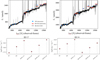 |
Fig. 4. Example of a simultaneous BEAGLE fit to HST photometry (top panel) and MUSE integrated fluxes (bottom panel) for the Mg II emitter ID17 at z = 0.84 (left panel) and Mg II absorbers ID14 at z = 0.77 (right panel). Top panel: HST (cyan diamonds) and predicted (black points and shaded red area) broad-band photometry. In black we show the full SED predicted from the BEAGLE fit. Bottom panel: integrated fluxes measured from MUSE spectra (red diamonds) and from the SED predicted by BEAGLE (gray diamonds). Error bars on the data points are contained within the markers. |
Stellar mass and star formation
Figure 5 shows the stellar mass versus SFR sequence for the Mg II parent sample. The typical (median) errors on stellar mass and SFR range from ∼±7% to ∼±15%, and from ∼±12% to ∼±24%, respectively. For reference, we report the star formation sequence by Whitaker et al. (2014) for 0.5 < z < 1.0 and 1.5 < z < 2.0 (solid and dotted dark red curves, respectively) derived from a mass-complete sample of star-forming galaxies in the CANDELS fields, drawn from the 3D-HST photometric catalogs. Specifically, we used the polynomial fit coefficients that parameterize the evolution of the SFR-stellar mass sequence reported in Table 1 of Whitaker et al. (2014). We also show the star formation sequence at z ∼ 0.9 from Eq. (11) of Boogaard et al. (2018, dashed dark blue line) computed using MUSE observations of the Hubble Ultra Deep Field and the Hubble Deep Field South of a sample of galaxies at 0.11 < z < 0.91, with stellar masses between 107 and 1010.5 M⊙.
Similarly to previous findings, we found Mg II emitters to exhibit on average lower stellar masses than the absorbers (see histograms in Fig. 5). The median values of stellar mass are 5.9 × 10⁸ M⊙ and 1.6 × 10¹⁰ M⊙ for Mg II emitters and absorbers, respectively. A two-sample KS test gives a p-value lower than 10−18, so that we chose to reject the null hypothesis that the two samples have the same stellar mass distributions. Analogous results were also found by previous works: Erb et al. (2012) on a sample drawn from a survey carried out with the LRIS spectrograph (LRIS-B) on the Keck I Telescope (Steidel et al. 2004), Kornei et al. (2013) in star-forming galaxies at z ∼ 1 from the DEEP2 survey, and by Finley et al. (2017b) in a subsample of this Mg II parent sample. Here we further confirm these previous findings by merely selecting our sources on the Mg II line, without any previous selection on photometric colors or other emission lines. We note that MUSE has allowed us to probe Mg II emission in galaxies with stellar masses one up to two orders of magnitude lower than those explored in the previous studies of Erb et al. (2012) and Kornei et al. (2013).
The Mg II absorbers also reach higher values of SFR, and lower values of sSFR, than emitters. Figure 5 is in overall agreement with Fig. 3 of Finley et al. (2017b), where stellar masses and SFR were obtained with two different methods (spectral fitting and an empirical relation using [O II]-dust corrected). It is worth noting that despite some quantitative differences between the SFR inferred from BEAGLE and those obtained with other methods, the general trends remain unchanged. Interestingly, galaxies with an Mg II P-Cygni profile show intermediate properties between emitters and absorbers and will be subject of future studies.
Before proceeding with the interpretation of the results, we need to consider the potential biases introduced by our sample selection. Mg II absorbers are on average more luminous than Mg II emitters because the ability to detect absorption features depends on the strength of the continuum. Moreover, the detection of continuum-faint Mg II emitters at z > 1.5 is complicated by skyline residuals. We performed a first test by dividing the sample into two redshift bins, 0.7 < z ≤ 1.5 and 1.5 < z ≤ 2.34, and then selecting Mg II emitters and absorbers within a given range of continuum luminosities in the F606W band.
The lower redshift bin, 0.7 < z < 1.5, had more than ten sources per Mg II spectral type (emitter and absorber) in the range of luminosity 23.3 < F6060W < 24.8 (where 23.3 is the brightest common magnitude between Mg II emitters and absorbers in the redshift range of interest, and 24.8 is the peak value of F6060W distribution of the Mg II absorbers), allowing for a statistical comparison. The F606W flux distributions of Mg II emitters and absorbers for the lower redshift bin are shown in Fig. 6 (left panel). The right panel of Fig. 6 shows that the Mg II emitters and absorbers within the selected range of F606W continuum fluxes (yellow shaded area in Fig. 6, left panel) still show a dichotomy in stellar mass.
The p-value from a two-sample KS test for this subsample is lower than 2 × 10⁻⁴ and allows us to reject the null hypothesis that the two mass distributions are the same. We obtained the same result when considering HST F775W. The higher redshift bins unfortunately have low number statistics. The number of galaxies with 1.5 < z ≤ 2.34 and within a common range of luminosity is limited to five absorbers and nine emitters. We still performed a two-sample KS test and found p-values lower than 0.008 both for HST F606W and HST F775W. This suggests that even though our sample is likely not to be complete in terms of low-luminosity Mg II absorbers (see Sect. 2), selection effects alone do not seem to be the primary driver for the difference in stellar mass between Mg II absorbers and emitters (Finley et al., in prep.).
 |
Fig. 5. Main sequence, SFR versus stellar mass, for the Mg II parent sample. We observe a smooth transitions in stellar mass from Mg II emitters (filled cyan triangles), to P-Cygni (filled green pentagons), to absorbers (empty magenta diamonds). Gray circles are Mg II non-detections. We also show the main-sequence curves from Boogaard et al. (2018), for z ∼ 0.9 (dashed dark blue line), and Whitaker et al. (2014) for 0.5 < z < 1.0 and 1.5 < z < 2.0 (solid and dotted dark red curves, respectively). |
 |
Fig. 6. Left panel: F606W passband filter flux distribution for Mg II emitters and absorbers (cyan and magenta histograms, respectively) in the redshift range 0.7 < z < 1.5. Right panel: stellar mass distributions of Mg II emitters and absorbers (same color-code as the left panel) with a given range of F606W flux, as highlighted in yellow in the left panel. |
Equivalent width of Mg II
Figure 7 shows the EW of the Mg IIλ2796 doublet component (computed with PLATEFIT as described in Sect. 2.1) versus stellar mass (left), inferred from the fit and UV absolute magnitude at 1600 Å (right), computed on the SED predicted by BEAGLE for Mg II absorbers and emitters that are defined to have EW Mg II > + 1 and < −1, respectively (see Sect. 2.3). Mg II emitters with high masses do not have strong Mg IIλ2796 EW in emission (left panel of Fig. 7). This could be explained in a scenario where as the amount of the ISM increases with stellar mass, the emission diminishes until it becomes completely suppressed, as we discuss in Sect. 5. Moreover, there is a lack of strong Mg IIλ2796 EW in emission for the bright (right panel of Fig. 7) Mg II emitters.
Mg II is very sensitive to emission infill (e.g., Prochaska et al. 2011; Scarlata & Panagia 2015; Zhu et al. 2015; Finley et al. 2017b), which is due to re-emission of photons of the same wavelength of the transition (Mg II λλ2796, 2803 in this case) that fills in the absorption profile. To correct EW measurements of Mg II for emission infill, Zhu et al. (2015) proposed an observation-driven method that consists of comparing EW of Mg II and Fe II λ2344, λ2374, λ2586, and λ2600 detected in quasar absorption-line systems to those observed in the spectra of star-forming galaxies. We do not cover the Fe II transitions for the entire sample, and we do not aim here at quantitatively discussing the EW measurements for Mg II absorbers. We note, however, that corrections for emission infill for the most massive sources would increase the EW of Mg II absorbers shown in Fig. 7 by values between 1.6 and 3 Å (Finley et al. 2017b, and in prep.). These corrections will introduce additional dispersion to Fig. 7, but will not affect the results discussed in Sect. 5.
 |
Fig. 7. EW of MGIIB for Mg II emitters (cyan triangles) and absorbers (magenta diamonds) as function of the stellar mass (left panel) and UV absolute magnitude at 1600 Å (right panel), color-coded accordingly to the redshift. The gray shaded area indicates the threshold values used to identify Mg II emitters (EW < −1.0) and absorbers (EW > 1.0). |
Dust attenuation, UV spectral slope, and ionizing emissivity
The dust attenuation at 1500 Å, A1500, inferred from the fitting, is on average higher for Mg II absorbers, with a median value of ∼1,52 compared to the ∼0.38 mag of the emitters. Kornei et al. (2013) also found galaxies with strong Mg II emission to have lower dust attenuation than their whole sample.
From the SED predicted from the BEAGLE fits, we computed the UV spectral slope β (defined as Fλ ∝ λβ) following the parametrization of Calzetti et al. (1994) and the intrinsic (not corrected for dust attenuation) UV luminosity at 1600 Å, MUV. As the spectral slope is particularly sensitive to the dust content within the galaxy, we expect the UV slopes to be on average bluer for Mg II emitters than absorbers. This is shown in Fig. 8, color-coded accordingly to the dust attenuation. Mg II emitters have a UV spectral slope β < −1, with a median value of ∼−1.98, for a wide range of UV luminosities (−21.0 < MUV < −16.6).
The Mg II absorbers, which are on average UV-brighter than emitters in our sample (Sect. 2.2), are also more massive (Sect. 2.4) and have redder UV spectral slopes with increasing UV luminosity. At fixed UV luminosity, Mg II emitters have bluer spectral slopes than absorbers. This is in agreement with previous findings from Erb et al. (2012), even though their Mg II emitters also included sources with P-Cygni profiles, which do not show any particular trend in Fig. 8 but lie in between Mg II emitters and absorbers.
From the BEAGLE fits, we inferred the ionizing emissivity, that is, the number of ionizing photons per UV luminosity. We computed two different ionizing emissivities considering the unattenuated and attenuated UV luminosity, as follows:
-
(i)
ξion stellar computed using only the unattenuated stellar UV luminosity, that is, ignoring the absorption and re-emission of photons inside the photoionization regions and dust attenuation;
-
(ii)
ξion computed using the total attenuated UV flux, that is, the photons that remain after the transfer of the stellar radiation through H II regions and interstellar dust, across a 100 Å window centered at λ = 1500 Å.
Figure 9 shows the distributions of the two ionizing emissivities, ξion stellar and ξion, for the whole sample. Mg II absorbers and emitters have similar distributions of the ionizing emissivity ξion stellar (left panel) computed on the unattenuated flux. When accounting for dust attenuation, Mg II emitters and absorbers show different distributions of the ionizing emissivity ξion (right panel), with Mg II emitters strongly peaking at lower values of ξion. Mg II absorbers, on the other hand, reach higher values of ξion. The errors associated with the ξion values are on the order of 0.1–0.2 dex, which is relatively large considering the small range of values concerned (Fig. 9). This is because the fit is, in most of the cases, constrained by the HST broad-band continuum and a few emission lines. It is worth highlighting that the ξion values shown here are not directly comparable with the values derived purely from nebular emission lines. ξion is commonly estimated from (dust-corrected) hydrogen recombination lines (e.g., Bouwens et al. 2016; Schaerer et al. 2016; Matthee et al. 2017; Harikane et al. 2018; Shivaei et al. 2018), and alternatively, by exploiting UV emission lines and photoionization models (e.g. Stark et al. 2015b, 2017; Nakajima et al. 2018a). Additional lines are required to further constrain this physical quantity for our sample. Moreover, the productions of ionizing photons is connected with the properties of the stellar populations (age, metallicity, and inclusion of binary stars) and with the escape fraction of ionizing photons (see Sect. 4 of Nakajima et al. 2018a, for a discussion of the uncertainties related to the interpretation of ξion). We focus here on a qualitative comparison of the distributions of ξion stellar and ξion, which mainly reflect the different dust attenuation experienced by Mg II emitters and absorbers.
The ionizing emissivity depends on the age and metallicity of the stellar populations. We did not find differences in the age and metallicity distributions of the Mg II emitters and absorbers, probably because of the relatively large redshift range explored here and the high number of free parameters. In the case of an equal release of ionizing photons, the ionizing emissivity depends only on the UV luminosity. Since the intrinsic (stellar) emissivity, ξion stellar, is similar for Mg II emitters and absorbers, the higher ξion reached by the Mg II absorbers can be explained in terms of lower (i.e., more attenuated by dust) observed UV luminosity. This implies that the ionizing source (i.e., stellar) in Mg II absorbers and emitters is intrinsically similar and that the differences between the two are mainly due to different dust and neutral gas content in the galaxy ISM.
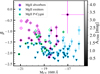 |
Fig. 8. UV spectral slope, β, versus UV absolute magnitude at 1600 Å and color-coded as function of the attenuation at 1500 Å, computed from the BEAGLE SED. Cyan triangles, green pentagons and magenta diamonds are Mg II emitters, P-Cygni and absorbers, respectively. |
 |
Fig. 9. Ionizing emissivity computed on the unattenuated stellar (left panel) and dust attenuated (right panel) UV luminosity, ξion stellar and ξion, respectively. Histograms are color-coded as labeled in the legend. |
5. Discussion
5.1. Predictions from photoionization models
Early theoretical works have predicted emission from the Mg II doublet in gaseous nebulae (e.g., Gurzadyan 1997, and references therein). Mg I is relatively easy to ionize, given its low-ionization potential of ∼7.65 eV, and electron collisions are efficient because of the low-excitation potential of the Mg II resonant level (∼4.4 eV). Dust can lead to a decrement of the emission line fluxes through absorption of photons. The associated photon scattering, within the ionized and neutral ISM, can give rise to the absorption features observed in galaxy spectra. The photoionization models of Gutkin et al. (2016) account for dust attenuation and resonant scattering effects within the H II regions, as CLOUDY uses a full treatment of optical depths and collisional excitation for multiple lines, including Mg II.
Figure 10 shows the effect of pure dust attenuation (i.e., without resonant scattering from the neutral ISM) beyond the H II regions on the Mg IIλ2796 intensities predicted by the models (solid lines). The predictions are for synthetic spectra of galaxies at z = 1 with M⋆ = 3 × 10⁹ M⊙ and three values of the SFR = 0.1, 1.0, 10.0 M⊙ yr−1 (color-coded as labeled in the legend), computed using the photoionization models of Gutkin et al. (2016; Sect. 3.1) and the BEAGLE code (Chevallard & Charlot 2016, see also Sect. 4.1). For consistency with the spectral fitting setup (described in Sect. 4), we assumed a delayed star formation history and Chabrier (2003) IMF with 100 M⊙ as upper mass cutoff. We adopted fixed values for the metallicity (Z = 0.5 Z⊙), the volume-averaged ionization parameter (log 〈U〉 = −2.0), and the dust-to-metal mass ratio (ξd = 0.3), in agreement with the average values found in Sect. 3.1. We applied the ISM dust attenuation model of Charlot & Fall (2000) to the predicted line fluxes, shown for different values of the dust optical depth in the V band, τV, in Fig. 10.
The Mg IIλ2796 line intensity starts to decrease at optical depth τV ∼ 0.1, with a steeper exponential decline at τV ≳ 1. The horizontal lines are the 3σ MUSE emission line flux detection limits for point-like sources (see Fig. 20 of Bacon et al. 2017) at 2800 Å (rest-frame) for mosaic (dashed line) and the deeper udf10 (continuous line). MUSE would detect the Mg II emission in galaxies with SFR ≥ 1 M⊙ yr−1; these values are consistent with our Fig. 5 and Fig. 3 of Finley et al. (2017b).
The fact that we do not observe the Mg II emission is related, along with dust absorption, to resonant scattering effects that are due to a higher amount of absorbing material in the neutral ISM. A higher amount of gas could then give rise to the Mg II absorption features observed in relatively massive and star-forming galaxies. Complementary information is needed to quantify gas masses of our Mg II emitters and absorbers. Unfortunately, detections of H I (tracer of the atomic gas) or CO (indirect tracer of the molecular gas H2) are not available for our sample. Neither can we constrain the gas mass from emission line fluxes as this requires the detection of the strongest optical emission lines from [O II]λλ3726; 3729 to [S II]λλ6717; 6731 (Brinchmann et al. 2013), which are not fully covered by our spectra.
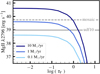 |
Fig. 10. Predictions of the Mg IIλ2796 line strength as a function of the galaxy dust attenuation, expressed in terms of the optical depth in the V band. These fluxes are for synthetic spectra of galaxies at z = 1 with M⋆ = 3 × 10⁹ M⊙ and SFR = 0.1, 1.0, 10.0 M⊙ yr−1, as labeled in the legend. Information about the other model parameters can be found in the text. The horizontal gray lines are the 3σ MUSE emission line flux detection limits for point-like sources at 2800 Å (rest-frame) for mosaic and udf10, dashed and continuous lines, respectively. |
5.2. Mg II emitters versus absorbers
Figure 5 shows a clear transition from Mg II emission to absorption in terms of stellar masses and SFR. Moreover, the structural analysis of HST observations has shown that Mg II emitters tend to have smaller sizes than absorbers (see also Finley et al. 2017b). This is consistent with the observational evidence that galaxy sizes increase with stellar mass (e.g., Shen et al. 2003; van der Wel et al. 2014). Furthermore, Mg II emitters have been found to have bluer spectral slopes than absorbers (Fig. 8), that is, a lower dust content. No particular trend has been found with redshift, metallicity, or other nebular properties, even though these could all be likely reasons for the observed scatter in the stellar mass–SFR relation shown in the middle panel of Fig. 5. As a different dust content also translates into a different amount of neutral gas, the observed Mg II transition from emission to absorption can be explained by the effect of the resonant scattering on the observed flux. The larger the amount of neutral gas in the ISM, the more strongly are the photons scattered resonantly within the medium, and hence, the higher the probability that they are absorbed by dust.
Our sources are also included in the CANDELS multiwavelength catalog of Guo et al. (2013). This catalog combines the Cosmic Assembly Near-infrared Deep Extragalactic Legacy Survey (CANDELS; Grogin et al. 2011; Koekemoer et al. 2011) HST/WFC3 F105W, F125W, and F160W data with existing public data, including the Spitzer/IRAC 3.6, 4.5, 5.8, and 8.0 μm fluxes. Figure 11 shows the flux ratio from the IRAC 3.6 and HST F160W bands versus redshift. Despite the large error bars for faint Mg II emitters, Mg II absorbers show redder F160W−3.6 μm colors than Mg II emitters. The physical interpretation of the rest-frame 1–2 μm near-infrared emission from star-forming galaxies is challenging, as it depends on the nature of the stars (most likely post-AGB stars) that contribute to it (e.g., Eminian et al. 2008). However, redder near-infrared colors have been observed in more star-forming systems, that is, higher SFR and stellar masses (e.g., Rodighiero et al. 2007; Eminian et al. 2008; Mentuch et al. 2010; Lange et al. 2016). The redder F160W−3.6 μm colors observed for the Mg II absorbers are in agreement with their higher stellar masses and SFR, as shown in Fig. 5.
 |
Fig. 11. IRAC 3.6 μm and HST F160W flux ratio vs. redshift for the Mg II emitters (cyan triangle), P-Cygni (green pentagons), and absorbers (magenta diamonds). Error bars on Mg II emitters and P-Cygni are contained within the markers. |
5.3. Mg II as an analog to Lyα
In Fig. 7 we observed a trend between the Mg II EW and the stellar mass (left) and UV luminosity (right) of our Mg II emitters. A deficit of bright Mg II emitters with strong emission Mg II EW (≲−7 Å) is observed. This result is similar to findings from previous studies on the resonant Lyα line. There is observational evidence (e.g., Ando et al. 2006; Stark et al. 2010; Furusawa et al. 2016; Hashimoto et al. 2017) for a lack of strong Lyα emission (EW < −100 Å) observed for UV bright (hence, more massive) sources, referred to as the “Ando-effect” (Ando et al. 2006). Multiple physical explanations can be invoked to describe the effect, including the neutral gas content, different dust attenuation, gas kinematics, and age of the stellar populations (Ando et al. 2006; Verhamme et al. 2008; Garel et al. 2012). Alternatively, Nilsson et al. (2009) argued that the deficit of high Lyα EW luminous galaxies is related to the rarity of these sources. Mg II and Lyα are resonant lines, so we should expect to observe some comparable trends (as argued also by Erb et al. 2012; Martin et al. 2013; Rigby et al. 2014; Henry et al. 2018), and the previous explanations to apply to Mg II as well. Guaita et al. (2011) found their faint high EW Lyα emitters (LAE) to have stellar masses lower than 1010 M⊙ and a lower dust content than in the brighter galaxies in their sample. In addition, Guaita et al. (2011) and Hathi et al. (2016) found Lyα emitters (EW ≥ 20 Å) at 2 < z < 2.5 to be less massive, to have a lower SFR, and less dust. Galaxies with strong Lyα emission have also been found to have smaller sizes than those with weaker emission or Lyα in absorption (e.g., Law et al. 2012; Shibuya et al. 2014; Kobayashi et al. 2016; Paulino-Afonso et al. 2018). These trends are similar to those observed between our fainter, low-mass, less dusty, small size Mg II emitters and brighter, more massive, dust-rich, larger size Mg II absorbers. In this respect, our results suggest that the lack of bright (and massive) Mg II emitters with strong emission Mg II EW (highly negative EW values) could be associated with an increased amount of the ISM within the galaxy itself, invoked to explain similar trends for the Lyα (e.g., Hashimoto et al. 2017).
5.4. Mg II escape fraction
Mg II photons within H II regions can resonantly scatter through the surrounding medium until they are absorbed by dust. The fraction of Mg II photons that escape the galaxy, fesc (Mg II), provides important clues on the effect of dust on resonant lines. This fraction is defined as the ratio between the Mg II observed flux and the intrinsic Mg II nebular emission (analogous to the escape fraction of Lyα, Verhamme et al. 2008; Hayes et al. 2010, 2011; Blanc et al. 2011; Atek et al. 2014). This ratio is equal to unity in absence of absorption; the lower its value, the higher the number of photons absorbed by dust grains.
From a study of ten local Green Pea galaxies, Henry et al. (2018) found the escape fraction of Mg II photons to closely correlate with that of Lyα photons, suggesting that both lines arise from the same low column density ISM gas. Henry et al. (2018) proposed a prescription, calibrated on photoionization models, to predict the intrinsic Mg II emission from the [O II] and [O III] line fluxes. Unfortunately, the MUSE spectral coverage does not enable us to observe these two lines simultaneously in our studied redshift range. Only 8 spectra of our 63 Mg II emitters exhibit both [O II] and [O III].
We estimated the Mg II escape fraction of our Mg II emitters from the ratio between the Mg IIλ2796 fluxes, computed using PLATEFIT (i.e., including correction for stellar absorption), and the Mg IIλ2796nebular flux from the photoionization models included in the BEAGLE fit. The observed Mg IIλ2796fluxes are dereddened using the optical depth inferred by the BEAGLE fit. Results are illustrated in Fig. 12. For comparison purpose, we also show the escape fraction computed assuming a Calzetti et al. (2000) attenuation curve. The fesc (Mg II) is lower than unity within errors for 73% (46/63) of our sample. For 38 of 63 sources with fesc (Mg II) < 1, the escape fraction ranges from 3 to 98%, with a median value of ∼54%. We note that Mg II emitters with dust optical depths, τd 2796, higher than unity have the lowest values of Mg II escape fraction, resembling the observed decrease in Lyα escape fraction with reddening E(B – V) (e.g., Hayes et al. 2010, 2011; Blanc et al. 2011; Atek et al. 2014). Despite the large number of variables that control the computation of fesc, as discussed below, our results lie around the dust attenuation curve of Calzetti et al. (2000), which corresponds to pure dust attenuation. This suggests little effect by resonant scattering on the observed fluxes of our Mg II emitters and therefore a low content of neutral gas. In addition, by comparing the fesc (Mg II) with the observed EW of Mg IIλ2796 and the intrinsic nebular Mg IIλ2796 flux from photoionization models, we found trends similar to those observed by Henry et al. (2018, see also their Fig. 5). Specifically, high fesc (Mg II) is not always associated with a strong observed Mg II emission. The strongest Mg II emitters (in terms of Mg IIλ2796 EW) of our sample are those with the weakest intrinsic nebular Mg IIλ2796 flux. These findings are in agreement with the interpretation by Henry et al. (2018) that strong Mg II emission is not uniquely associated with a higher production of Mg II photons but is rather observed when Mg II photons can escape the ISM.
The reasons for observing fesc (Mg II) higher than unity are multifold, arising from both uncertainties on the observed quantities and assumptions on the modeling approach. Firstly, the spectral fitting procedure described in Sect. 4 is complex as it aims at reproducing the full SED of our galaxies, accounting simultaneously for the continuum (from stars and gas) and nebular emissions. The HST photometric bands provide strong constraints on the choice of models, in particular in the cases where only few emission lines are detected. For instance, seven of the sources (at z > 1.49) for which the only line detected is the C III] doublet have fesc (Mg II) > 1. In contrast, the majority of the sources (at z < 0.86) with the highest number of emission lines detected, including [O III]λ5007, have fesc (Mg II) < 1 (orange contoured triangles in Fig. 12). Clearly, the computation of the Mg II escape fraction benefits from additional information on optical emission lines, to better constrain the nebular properties (as also discussed in Sect. 3.3).
A second reason is related to a possible extended Mg II emission, similar to that observed for Lyα (e.g., Herenz et al. 2015; Wisotzki et al. 2016; Drake et al. 2017; Leclercq et al. 2017; Marino et al. 2018) and Fe II* (Finley et al. 2017a). If this is case, the observed emission line ratios might be altered by the approach that is chosen to estimate the line flux (see Sect. 4.1 of Drake et al. 2017). Furthermore, given the low ionization and excitation potential of Mg II (∼7.65 eV and ∼4.4 eV, respectively), its emission might extend beyond the outer radius of the photoionization calculations3. Effects related to shocks, compression, and turbulence within the medium could also provide an additional contribution to the Mg II observed flux. Geometrical effects, that is, the angular distribution of Mg II photons due to resonant scattering, might be another contributing factor. Follow-up studies should therefore focus on modeling the emission of resonant low-ionization lines beyond the hydrogen ionization front and on comparing the spatially resolved emission from Mg II to that of other non-resonant lines, such as [O II] and C III] (see also Martin et al. 2013).
It is also worth mentioning that Mg II is a refractory element and is therefore sensitive to the level of depletion onto dust grains (Guseva et al. 2013). In the Gutkin et al. (2016) models, ∼20% up to ∼80% of Mg II is confined in dust. This range is consistent with ∼50% of magnesium depleted onto dust grains found by Guseva et al. (2013). This therefore is probably not the main explanation for fesc (Mg II) > 1. However, this and any other dependence on model assumptions needs to be taken into account when observations are compared with theoretical predictions. This is particularly true for high-redshift sources, as their dust properties can differ from local sources (Cucciati et al. 2012), and models might require a finer tuning.
Finally, we note that PLATEFIT uses templates (i.e., Bruzual & Charlot 2003) to subtract the stellar continuum that are different from those used in BEAGLE (i.e., Bruzual & Charlot in prep.). In their work on low-redshift sources, Guseva et al. (2013) applied a constant correction for the stellar continuum to the observed fluxes (by multiplying the line intensities for (EW + 0.5)/EW), motivated by the roughly constant Mg II stellar features in the models (i.e., Bruzual & Charlot 2003) over a wide range of stellar ages. Similarly, Henry et al. (2018) applied a 0.3 Å correction to the EW of each Mg II doublet component. Given the small extent of this correction, we expect the differences among templates to play a secondary role.
To conclude, we caution about any quantitative study of the Mg II escape fraction, given the complexity from the observational and theoretical side of controlling its estimate. However, even if further work is required, we emphasize the potential use of Mg II as complementary and, hopefully, alternative, resonant line to the better studied Lyα. Even if much fainter, Mg II is less affected by the absorption of the intergalactic medium than Lyα (Henry et al. 2018).
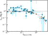 |
Fig. 12. Mg II escape fraction as function of the optical depth at the Mg IIλ2796 wavelength for our Mg II emitters. Orange contoured triangles are Mg II emitters at z < 0.86. The salmon curve shows the Calzetti et al. (2000) attenuation curve. |
6. Summary and conclusions
We have studied a sample of 381 galaxies in the MUSE Hubble Ultra Deep Field Survey (Bacon et al. 2017) within a redshift range of 0.7 < z < 2.34. Of these, 123 galaxies show a wide variety of Mg II λλ2796, 2803 doublet profiles, ranging from emission to absorption, and they were classified into Mg II emitters (63), Mg II P-Cygni (19), and Mg II absorbers (41). The main goal of this work was to find the underlying physical properties that drive the detection of the Mg II doublet in emission or in absorption in the spectra of galaxies up to the peak of the SFRD history (Madau & Dickinson 2014), where a change in the regime of the global properties (also in terms of dust content, Cucciati et al. 2012) of star-forming galaxies is observed. We summarize the main results of this work below and highlight future prospectives.
We first explored whether the line fluxes of Mg II emitters are consistent with predictions from nebular emission in star-forming galaxies (Fig. 3) and found them to be compatible with ionizing photons produced within H II regions (see also Erb et al. 2012).
Based on the measured emission line ratios available in our sample (i.e., [O II]/Mg II, [Ne III]/Mg II and C III]/Mg II), we were not able to identify features that would enable us to confirm or reject AGN or radiative shocks as ionization sources. However, we removed all the potential AGN identified through X-ray from our sample (see Sects. 2.2 and 3.3), and we do not expect our Mg II emitters to be contaminated by strong AGN. While we can dismiss a substantial contribution from gravitational accretion onto black holes, we cannot rule out a possible contamination from shocks in the observed spectra.
To explore whether the different profiles of the Mg II doublet trace particular properties of the galaxies, we relied on the Bayesian spectral fitting code BEAGLE (Chevallard & Charlot 2016). Specifically, we exploited the information from MUSE spectra and HST broad-band photometry and performed a spectral fit accounting simultaneously for the continuum and nebular stellar emissions (examples are shown in Fig. 4). We found Mg II emitters to have on average lower stellar masses and bluer spectral slopes (i.e., lower dust attenuation) than Mg II absorbers (Figs. 5, 8, and 9). This indicates that the content of dust and neutral gas in the ISM of our galaxies plays a dominant role in shaping the Mg II features.
We found a lack of strong Mg II EW in emission for our bright Mg II emitters (Fig. 7), similar to the trend that has been observed for Lyα. As they are both resonant lines, we would expect to find correlations between the observed properties of Mg II and Lyα, upon the assumptions that the source of photons production is the same and that they are observed through the same medium.
We computed the fraction of Mg II photons escaping the galaxy (Fig. 12), finding many uncertainties in deriving this quantity. These uncertainties are mainly related to our modeling approach and other physical processes that could come into play (e.g., shocks or geometrical effects). Additional spectral information (preferentially spatially resolved) and a tailored modeling of the Mg II resonant doublet are necessary to fully understand its emission feature. Nevertheless, extending the escape fraction studies, until now mainly restricted to the Lyα line (e.g., Verhamme et al. 2008; Hayes et al. 2010, 2011; Blanc et al. 2011; Atek et al. 2014), with other resonant lines, such as Mg II, is a promising approach to better understand the physics of the ISM within galaxies (see also Henry et al. 2018).
Additional emission lines in the rest-frame UV/optical range, along with deep spatially resolved spectroscopy, are required to further investigate the physical origin of Mg II emission. This is especially relevant for sources whose observed Mg II flux is higher than the flux predicted by purely nebular emission and for studying the potential effect of radiative shocks on the observed spectra of our Mg II emitters. In particular, the completion of deeper MUSE observations with adaptive optics, planned for a subregion of 1 square arcminute of the UDF, will enable further studies in this direction. We expect new data for at least 34 of the 381 galaxies of our sample (including six Mg II emitters, two P-Cygni, and two absorbers).
Most likely, a contribution from shocks is present in sources with Mg II P-Cygni-like profiles, as this peculiar profile is a tracer of galactic winds. A detailed study of the Mg II spectral shape and physical properties of these sources is beyond the scope of this paper and will be subject of future analysis. It is worth highlighting that galaxies with an Mg II P-Cygni profile show intermediate properties between emitters and absorbers. Additional studies of Mg II P-Cygni will help us understand whether Mg II emitters are the results of a complete “blowout” of gas from galactic winds or if their stellar populations have simply fully ionized the gas. In this respect, we note that six of our Mg II emitters (ID 84, 121, 46, 92, 1219, and 7101) are in major close pairs (Table 3 of Ventou et al. 2017), pointing to major mergers. These merging events may indeed have produced galactic outflows for these sources (see also Finley et al. 2017b). Follow-up studies will focus on explaining the observed transitions between Mg II in emission, through the P-Cygni profile, to absorption by means of proper radiative transfer modeling of the neutral medium (Garel et al., in prep.; Finley et al., in prep.).
Our spectral modeling accounts for photospheric stellar emission and absorption and for the nebular emission from ionized gas, but does not include the effect of the neutral ISM. Spectral models incorporating absorption by neutral gas have been developed by Vidal-García et al. (2017) and are now being implemented wihin the fitting code BEAGLE to achieve a more comprehensive and simultaneous treatment of the spectral features from stars and ionized and neutral ISM in and around galaxies.
To conclude, pushing these studies to higher redshift will allow us to determine whether Mg II emitters are common or rare at earlier epochs. The Mg II line doublet is also very promising because it undergoes the same physics as the Lyα line because of their resonant nature. A close connection between the profiles of these two lines has recently been found in Green Peas galaxies at z ∼ 0.2 – 0.3 (Henry et al. 2018). It would be extremely interesting to see whether a connection exists between the properties of these two lines up to earlier epochs of galaxy evolution. One possibility is to search for Mg II emission in near-infrared spectroscopic observations complementary those of the MUSE LAE. For example, K-band Multi-Object Spectrometer (KMOS) observations are available for the MUSE-Wide LAE and 3D-HST grism spectroscopy for the MUSE UDF. Moreover, future near-infrared spectrographs, such as NIRSpec on board the James Webb Space Telescope, might also enable studies of the Mg II features at higher redshifts than those explored in this work, along with the simultaneous observations of Lyα for the most distant sources. This will provide additional clues on the dust and gas content of the ISM at high redshifts and, why not, during the reionization epoch.
GALFIT homepage: https://users.obs.carnegiescience.edu/peng/work/galfit/galfit.html
The CLOUDY calculations in the Gutkin et al. (2016) models stop when the electron density decreases below 1% of the hydrogen density or if the temperature falls to below 100 K.
Acknowledgments
AF thanks Emma Curtis-Lake and Alba Vidal-García for valuable input on SED modeling and fitting. This work is supported by the ERC advanced grant 339659-MUSICOS (R. Bacon). This work makes use of the MUSE Python Data Analysis Framework, MPDAF (https://git-cral.univ-lyon1.fr/MUSE/mpdaf), developed at the Centre de Recherche Astrophysique de Lyon (CRAL). LT and AF thank Baptiste Pellorce for his contribution during his UCBL1 undergrade internship at CRAL. DC and JR acknowledge support from the ERC starting grant 336736-CALENDS. SC and JC acknowledge financial support from the European Research Council via an Advanced Grant under grant agreement no. 321323 (NEOGAL). TC acknowledges support of the ANR FOGHAR (ANR-13-BS05-0010-02), the OCEVU Labex (ANR-11-LABX-0060), and the A*MIDEX project (ANR-11-IDEX-0001-02) funded by the “Investissements d’avenir” French government program. JB acknowledges support by Fundação para a Ciência e a Tecnologia (FCT) through national funds (UID/FIS/04434/2013) and by FEDER through COMPETE2020 (POCI-01-0145-FEDER-007672) and Investigador FCT contract IF/01654/2014/CP1215/CT0003.
References
- Aguirre, A., Hernquist, L., Schaye, J., et al. 2001, ApJ, 561, 521 [NASA ADS] [CrossRef] [Google Scholar]
- Ali, B., Blum, R. D., Bumgardner, T. E., et al. 1991, PASP, 103, 1182 [NASA ADS] [CrossRef] [Google Scholar]
- Allen, M. G., Groves, B. A., Dopita, M. A., Sutherland, R. S., & Kewley, L. J. 2008, ApJ, 178, 20 [NASA ADS] [Google Scholar]
- Ando, M., Ohta, K., Iwata, I., et al. 2006, ApJ, 645, L9 [NASA ADS] [CrossRef] [Google Scholar]
- Atek, H., Kneib, J.-P., Pacifici, C., et al. 2014, ApJ, 789, 96 [NASA ADS] [CrossRef] [Google Scholar]
- Bacon, R., Brinchmann, J., Richard, J., et al. 2015, A&A, 575, A75 [NASA ADS] [CrossRef] [EDP Sciences] [Google Scholar]
- Bacon, R., Conseil, S., Mary, D., et al. 2017, A&A, 608, A1 [NASA ADS] [CrossRef] [EDP Sciences] [Google Scholar]
- Berg, D. A., Skillman, E. D., Henry, R. B. C., Erb, D. K., & Carigi, L. 2016, ApJ, 827, 126 [NASA ADS] [CrossRef] [Google Scholar]
- Berg, D. A., Erb, D. K., Auger, M. W., Pettini, M., & Brammer, G. B. 2018, ApJ, 859, 164 [NASA ADS] [CrossRef] [Google Scholar]
- Blanc, G. A., Adams, J. J., Gebhardt, K., et al. 2011, ApJ, 736, 31 [NASA ADS] [CrossRef] [Google Scholar]
- Boogaard, L., Brinchmann, J., Bouché, N., et al. 2018, A&A, in press, DOI: 10.1051/0004-6361/201833136 [Google Scholar]
- Bordoloi, R., Rigby, J. R., Tumlinson, J., et al. 2016, MNRAS, 458, 1891 [NASA ADS] [CrossRef] [Google Scholar]
- Bouwens, R. J., Smit, R., Labbé, I., et al. 2016, ApJ, 831, 176 [NASA ADS] [CrossRef] [Google Scholar]
- Brammer, G. B., van Dokkum, P. G., Franx, M., et al. 2012, ApJ, 200, 13 [NASA ADS] [CrossRef] [Google Scholar]
- Bressan, A., Marigo, P., Girardi, L., et al. 2012, MNRAS, 427, 127 [NASA ADS] [CrossRef] [Google Scholar]
- Brinchmann, J., Charlot, S., White, S. D. M., et al. 2004, MNRAS, 351, 1151 [NASA ADS] [CrossRef] [Google Scholar]
- Brinchmann, J., Pettini, M., & Charlot, S. 2008, MNRAS, 385, 769 [NASA ADS] [CrossRef] [Google Scholar]
- Brinchmann, J., Charlot, S., Kauffmann, G., et al. 2013, MNRAS, 432, 2112 [NASA ADS] [CrossRef] [Google Scholar]
- Bruzual, G., & Charlot, S. 2003, MNRAS, 344, 1000 [NASA ADS] [CrossRef] [Google Scholar]
- Calzetti, D., Kinney, A. L., & Storchi-Bergmann, T. 1994, ApJ, 429, 582 [NASA ADS] [CrossRef] [Google Scholar]
- Calzetti, D., Armus, L., Bohlin, R. C., et al. 2000, ApJ, 533, 682 [NASA ADS] [CrossRef] [Google Scholar]
- Chabrier, G. 2003, PASP, 115, 763 [Google Scholar]
- Charlot, S., & Fall, S. M. 2000, ApJ, 539, 718 [Google Scholar]
- Charlot, S., & Longhetti, M. 2001, MNRAS, 323, 887 [NASA ADS] [CrossRef] [Google Scholar]
- Chevallard, J., & Charlot, S. 2016, MNRAS, 462, 1415 [NASA ADS] [CrossRef] [Google Scholar]
- Chevallard, J., Charlot, S., Wandelt, B., & Wild, V. 2013, MNRAS, 432, 2061 [NASA ADS] [CrossRef] [Google Scholar]
- Chevallard, J., Charlot, S., Senchyna, P., et al. 2018, MNRAS, 479, 3264 [NASA ADS] [CrossRef] [Google Scholar]
- Cucciati, O., Tresse, L., Ilbert, O., et al. 2012, A&A, 539, A31 [NASA ADS] [CrossRef] [EDP Sciences] [Google Scholar]
- Drake, A. B., Guiderdoni, B., Blaizot, J., et al. 2017, MNRAS, 471, 267 [NASA ADS] [CrossRef] [Google Scholar]
- Eminian, C., Kauffmann, G., Charlot, S., et al. 2008, MNRAS, 384, 930 [NASA ADS] [CrossRef] [Google Scholar]
- Erb, D. K., Quider, A. M., Henry, A. L., & Martin, C. L. 2012, ApJ, 759, 26 [NASA ADS] [CrossRef] [Google Scholar]
- Feltre, A., Charlot, S., & Gutkin, J. 2016, MNRAS, 456, 3354 [Google Scholar]
- Ferland, G. J., Porter, R. L., van Hoof, P. A. M., et al. 2013, Rev. Mex. Astron. Astrofis., 49, 137 [Google Scholar]
- Finlator, K., & Davé, R. 2008, MNRAS, 385, 2181 [NASA ADS] [CrossRef] [Google Scholar]
- Finley, H., Bouché, N., Contini, T., et al. 2017a, A&A, 605, A118 [NASA ADS] [CrossRef] [EDP Sciences] [Google Scholar]
- Finley, H., Bouché, N., Contini, T., et al. 2017b, A&A, 608, A7 [NASA ADS] [CrossRef] [EDP Sciences] [Google Scholar]
- Furusawa, H., Kashikawa, N., Kobayashi, M. A. R., et al. 2016, ApJ, 822, 46 [NASA ADS] [CrossRef] [Google Scholar]
- Garel, T., Blaizot, J., Guiderdoni, B., et al. 2012, MNRAS, 422, 310 [NASA ADS] [CrossRef] [Google Scholar]
- Giavalisco, M., Vanzella, E., Salimbeni, S., et al. 2011, ApJ, 743, 95 [NASA ADS] [CrossRef] [Google Scholar]
- Grogin, N. A., Kocevski, D. D., Faber, S. M., et al. 2011, ApJ, 197, 35 [Google Scholar]
- Guaita, L., Acquaviva, V., Padilla, N., et al. 2011, ApJ, 733, 114 [NASA ADS] [CrossRef] [Google Scholar]
- Guo, Y., Ferguson, H. C., Giavalisco, M., et al. 2013, ApJ, 207, 24 [NASA ADS] [CrossRef] [Google Scholar]
- Gurzadyan, G. A. 1997, The Physics and Dynamics of Planetary Nebulae, XVI (Berlin, Heidelberg, New-York: Springer-Verlag) [CrossRef] [Google Scholar]
- Guseva, N. G., Izotov, Y. I., Fricke, K. J., & Henkel, C. 2013, A&A, 555, A90 [NASA ADS] [CrossRef] [EDP Sciences] [Google Scholar]
- Gutkin, J., Charlot, S., & Bruzual, G. 2016, MNRAS, 462, 1757 [NASA ADS] [CrossRef] [Google Scholar]
- Harikane, Y., Ouchi, M., Yuma, S., et al. 2014, ApJ, 794, 129 [NASA ADS] [CrossRef] [Google Scholar]
- Harikane, Y., Ouchi, M., Shibuya, T., et al. 2018, ApJ, 859, 84 [NASA ADS] [CrossRef] [Google Scholar]
- Hashimoto, T., Garel, T., Guiderdoni, B., et al. 2017, A&A, 608, A10 [NASA ADS] [CrossRef] [EDP Sciences] [Google Scholar]
- Hathi, N. P., Le Fèvre, O., Ilbert, O., et al. 2016, A&A, 588, A26 [NASA ADS] [CrossRef] [EDP Sciences] [Google Scholar]
- Hayes, M., Östlin, G., Schaerer, D., et al. 2010, Nature, 464, 562 [NASA ADS] [CrossRef] [PubMed] [Google Scholar]
- Hayes, M., Schaerer, D., Östlin, G., et al. 2011, ApJ, 730, 8 [NASA ADS] [CrossRef] [Google Scholar]
- Henry, A., Berg, D. A., Scarlata, C., Verhamme, A., & Erb, D. 2018, ApJ, 855, 96 [NASA ADS] [CrossRef] [Google Scholar]
- Herenz, E. C., Wisotzki, L., Roth, M., & Anders, F. 2015, A&A, 576, A115 [NASA ADS] [CrossRef] [EDP Sciences] [Google Scholar]
- Hirschmann, M., Charlot, S., Feltre, A., et al. 2017, MNRAS, 472, 2468 [NASA ADS] [CrossRef] [Google Scholar]
- Hummer, D. G., & Storey, P. J. 1987, MNRAS, 224, 801 [NASA ADS] [CrossRef] [Google Scholar]
- Inami, H., Bacon, R., Brinchmann, J., et al. 2017, A&A, 608, A2 [NASA ADS] [CrossRef] [EDP Sciences] [Google Scholar]
- Izotov, Y. I., Guseva, N. G., Fricke, K. J., & Henkel, C. 2016, MNRAS, 462, 4427 [NASA ADS] [CrossRef] [Google Scholar]
- Izotov, Y. I., Guseva, N. G., Fricke, K. J., Henkel, C., & Schaerer, D. 2017, MNRAS, 467, 4118 [NASA ADS] [CrossRef] [Google Scholar]
- Karman, W., Grillo, C., Balestra, I., et al. 2016, A&A, 585, A27 [NASA ADS] [CrossRef] [EDP Sciences] [Google Scholar]
- Kewley, L. J., Dopita, M. A., Leitherer, C., et al. 2013, ApJ, 774, 100 [NASA ADS] [CrossRef] [Google Scholar]
- Kinney, A. L., Bohlin, R. C., Calzetti, D., Panagia, N., & Wyse, R. F. G. 1993, ApJ, 86, 5 [NASA ADS] [CrossRef] [Google Scholar]
- Kobayashi, M. A. R., Murata, K. L., Koekemoer, A. M., et al. 2016, ApJ, 819, 25 [NASA ADS] [CrossRef] [Google Scholar]
- Koekemoer, A. M., Faber, S. M., Ferguson, H. C., et al. 2011, ApJ, 197, 36 [Google Scholar]
- Kornei, K. A., Shapley, A. E., Martin, C. L., et al. 2013, ApJ, 774, 50 [NASA ADS] [CrossRef] [Google Scholar]
- Lange, J. U., van Dokkum, P. G., Momcheva, I. G., et al. 2016, ApJ, 819, L4 [NASA ADS] [CrossRef] [Google Scholar]
- Laor, A., Jannuzi, B. T., Green, R. F., & Boroson, T. A. 1997, ApJ, 489, 656 [NASA ADS] [CrossRef] [Google Scholar]
- Law, D. R., Steidel, C. C., Shapley, A. E., et al. 2012, ApJ, 759, 29 [NASA ADS] [CrossRef] [Google Scholar]
- Leclercq, F., Bacon, R., Wisotzki, L., et al. 2017, A&A, 608, A8 [NASA ADS] [CrossRef] [EDP Sciences] [Google Scholar]
- Levesque, E. M., & Richardson, M. L. A. 2014, ApJ, 780, 100 [NASA ADS] [CrossRef] [Google Scholar]
- Lilly, S. J., Carollo, C. M., Pipino, A., Renzini, A., & Peng, Y. 2013, ApJ, 772, 119 [NASA ADS] [CrossRef] [Google Scholar]
- Luo, B., Brandt, W. N., Xue, Y. Q., et al. 2017, ApJ, 228, 2 [NASA ADS] [CrossRef] [Google Scholar]
- Madau, P., & Dickinson, M. 2014, ARA&A, 52, 415 [NASA ADS] [CrossRef] [Google Scholar]
- Mainali, R., Kollmeier, J. A., Stark, D. P., et al. 2017, ApJ, 836, L14 [NASA ADS] [CrossRef] [Google Scholar]
- Maiolino, R., Nagao, T., Grazian, A., et al. 2008, A&A, 488, 463 [NASA ADS] [CrossRef] [EDP Sciences] [Google Scholar]
- Mannucci, F., Cresci, G., Maiolino, R., et al. 2009, MNRAS, 398, 1915 [NASA ADS] [CrossRef] [Google Scholar]
- Marino, R. A., Cantalupo, S., Lilly, S. J., et al. 2018, ApJ, 859, 53 [NASA ADS] [CrossRef] [Google Scholar]
- Martin, C. L., Shapley, A. E., Coil, A. L., et al. 2012, ApJ, 760, 127 [NASA ADS] [CrossRef] [Google Scholar]
- Martin, C. L., Shapley, A. E., Coil, A. L., et al. 2013, ApJ, 770, 41 [NASA ADS] [CrossRef] [Google Scholar]
- Maseda, M. V., Brinchmann, J., Franx, M., et al. 2017, A&A, 608, A4 [NASA ADS] [CrossRef] [EDP Sciences] [Google Scholar]
- Matthee, J., Sobral, D., Best, P., et al. 2017, MNRAS, 465, 3637 [NASA ADS] [CrossRef] [Google Scholar]
- Mentuch, E., Abraham, R. G., & Zibetti, S. 2010, ApJ, 725, 1971 [NASA ADS] [CrossRef] [Google Scholar]
- Momcheva, I. G., Brammer, G. B., van Dokkum, P. G., et al. 2016, ApJ, 225, 27 [NASA ADS] [Google Scholar]
- Nagao, T., Maiolino, R., & Marconi, A. 2006, A&A, 459, 85 [NASA ADS] [CrossRef] [EDP Sciences] [Google Scholar]
- Nakajima, K., Fletcher, T., Ellis, R. S., Robertson, B. E., & Iwata, I. 2018a, MNRAS, 477, 2098 [NASA ADS] [CrossRef] [Google Scholar]
- Nakajima, K., Schaerer, D., Le Fèvre, O., et al. 2018b, A&A, 612, A94 [NASA ADS] [CrossRef] [EDP Sciences] [Google Scholar]
- Newman, J. A., Cooper, M. C., Davis, M., et al. 2013, ApJ, 208, 5 [NASA ADS] [CrossRef] [Google Scholar]
- Nilsson, K. K., Möller-Nilsson, O., Møller, P., Fynbo, J. P. U., & Shapley, A. E. 2009, MNRAS, 400, 232 [NASA ADS] [CrossRef] [Google Scholar]
- Panuzzo, P., Bressan, A., Granato, G. L., Silva, L., & Danese, L. 2003, A&A, 409, 99 [NASA ADS] [CrossRef] [EDP Sciences] [Google Scholar]
- Paulino-Afonso, A., Sobral, D., Ribeiro, B., et al. 2018, MNRAS, 476, 5479 [NASA ADS] [CrossRef] [Google Scholar]
- Peng, C. Y., Ho, L. C., Impey, C. D., & Rix, H.-W. 2010, AJ, 139, 2097 [NASA ADS] [CrossRef] [Google Scholar]
- Planck Collaboration XIII. 2016, A&A, 594, A13 [NASA ADS] [CrossRef] [EDP Sciences] [Google Scholar]
- Prochaska, J. X., Kasen, D., & Rubin, K. 2011, ApJ, 734, 24 [NASA ADS] [CrossRef] [Google Scholar]
- Rafelski, M., Teplitz, H. I., Gardner, J. P., et al. 2015, AJ, 150, 31 [NASA ADS] [CrossRef] [Google Scholar]
- Rich, J. A., Kewley, L. J., & Dopita, M. A. 2011, ApJ, 734, 87 [NASA ADS] [CrossRef] [Google Scholar]
- Rich, J. A., Kewley, L. J., & Dopita, M. A. 2014, ApJ, 781, L12 [NASA ADS] [CrossRef] [Google Scholar]
- Rigby, J. R., Bayliss, M. B., Gladders, M. D., et al. 2014, ApJ, 790, 44 [NASA ADS] [CrossRef] [Google Scholar]
- Rodighiero, G., Cimatti, A., Franceschini, A., et al. 2007, A&A, 470, 21 [NASA ADS] [CrossRef] [EDP Sciences] [Google Scholar]
- Rubin, K. H. R., Weiner, B. J., Koo, D. C., et al. 2010, ApJ, 719, 1503 [NASA ADS] [CrossRef] [Google Scholar]
- Rubin, K. H. R., Prochaska, J. X., Ménard, B., et al. 2011, ApJ, 728, 55 [NASA ADS] [CrossRef] [Google Scholar]
- Sánchez-Blázquez, P., Peletier, R. F., Jiménez-Vicente, J., et al. 2006, MNRAS, 371, 703 [NASA ADS] [CrossRef] [Google Scholar]
- Scarlata, C., & Panagia, N. 2015, ApJ, 801, 43 [NASA ADS] [CrossRef] [Google Scholar]
- Schaerer, D., Izotov, Y. I., Verhamme, A., et al. 2016, A&A, 591, L8 [NASA ADS] [CrossRef] [EDP Sciences] [Google Scholar]
- Senchyna, P., Stark, D. P., Vidal-García, A., et al. 2017, MNRAS, 472, 2608 [NASA ADS] [CrossRef] [Google Scholar]
- Shen, S., Mo, H. J., White, S. D. M., et al. 2003, MNRAS, 343, 978 [NASA ADS] [CrossRef] [Google Scholar]
- Shibuya, T., Ouchi, M., Nakajima, K., et al. 2014, ApJ, 785, 64 [NASA ADS] [CrossRef] [Google Scholar]
- Shirazi, M., & Brinchmann, J. 2012, MNRAS, 421, 1043 [NASA ADS] [CrossRef] [Google Scholar]
- Shivaei, I., Reddy, N. A., Siana, B., et al. 2018, ApJ, 855, 42 [NASA ADS] [CrossRef] [Google Scholar]
- Stark, D. P. 2016, ARA&A, 54, 761 [Google Scholar]
- Stark, D. P., Ellis, R. S., Chiu, K., Ouchi, M., & Bunker, A. 2010, MNRAS, 408, 1628 [NASA ADS] [CrossRef] [Google Scholar]
- Stark, D. P., Richard, J., Siana, B., et al. 2014, MNRAS, 445, 3200 [NASA ADS] [CrossRef] [Google Scholar]
- Stark, D. P., Richard, J., Charlot, S., et al. 2015a, MNRAS, 450, 1846 [NASA ADS] [CrossRef] [Google Scholar]
- Stark, D. P., Walth, G., Charlot, S., et al. 2015b, MNRAS, 454, 1393 [NASA ADS] [CrossRef] [Google Scholar]
- Stark, D. P., Ellis, R. S., Charlot, S., et al. 2017, MNRAS, 464, 469 [NASA ADS] [CrossRef] [Google Scholar]
- Stasińska, G., & Leitherer, C. 1996, ApJ, 107, 661 [NASA ADS] [CrossRef] [Google Scholar]
- Steidel, C. C., Shapley, A. E., Pettini, M., et al. 2004, ApJ, 604, 534 [NASA ADS] [CrossRef] [Google Scholar]
- Steidel, C. C., Erb, D. K., Shapley, A. E., et al. 2010, ApJ, 717, 289 [NASA ADS] [CrossRef] [Google Scholar]
- Tremonti, C. A., Heckman, T. M., Kauffmann, G., et al. 2004, ApJ, 613, 898 [NASA ADS] [CrossRef] [Google Scholar]
- Tremonti, C. A., Moustakas, J., & Diamond-Stanic, A. M. 2007, ApJ, 663, L77 [NASA ADS] [CrossRef] [Google Scholar]
- van der Wel, A., Bell, E. F., Häussler, B., et al. 2012, ApJ, 203, 24 [NASA ADS] [CrossRef] [Google Scholar]
- van der Wel, A., Franx, M., van Dokkum, P. G., et al. 2014, ApJ, 788, 28 [NASA ADS] [CrossRef] [Google Scholar]
- Vanzella, E., De Barros, S., Cupani, G., et al. 2016, ApJ, 821, L27 [NASA ADS] [CrossRef] [Google Scholar]
- Veilleux, S., Cecil, G., & Bland-Hawthorn, J. 2005, ARA&A, 43, 769 [Google Scholar]
- Ventou, E., Contini, T., Bouché, N., et al. 2017, A&A, 608, A9 [NASA ADS] [CrossRef] [EDP Sciences] [Google Scholar]
- Verhamme, A., Schaerer, D., Atek, H., & Tapken, C. 2008, A&A, 491, 89 [NASA ADS] [CrossRef] [EDP Sciences] [Google Scholar]
- Vidal-García, A., Charlot, S., Bruzual, G., & Hubeny, I. 2017, MNRAS, 470, 3532 [NASA ADS] [CrossRef] [Google Scholar]
- Weiner, B. J., Coil, A. L., Prochaska, J. X., et al. 2009, ApJ, 692, 187 [NASA ADS] [CrossRef] [Google Scholar]
- Whitaker, K. E., Franx, M., Leja, J., et al. 2014, ApJ, 795, 104 [NASA ADS] [CrossRef] [MathSciNet] [Google Scholar]
- Wisotzki, L., Bacon, R., Blaizot, J., et al. 2016, A&A, 587, A98 [NASA ADS] [CrossRef] [EDP Sciences] [Google Scholar]
- Wofford, A., Charlot, S., Bruzual, G., et al. 2016, MNRAS, 457, 4296 [NASA ADS] [CrossRef] [Google Scholar]
- York, D. G., Adelman, J., Anderson, Jr., J. E., et al. 2000, AJ, 120, 1579 [CrossRef] [Google Scholar]
- Yuan, T.-T., Kewley, L. J., Swinbank, A. M., & Richard, J. 2012, ApJ, 759, 66 [NASA ADS] [CrossRef] [Google Scholar]
- Zhu, G. B., Comparat, J., Kneib, J.-P., et al. 2015, ApJ, 815, 48 [NASA ADS] [CrossRef] [Google Scholar]
All Tables
All Figures
|
Fig. 1. Zoom-in of MUSE spectra at rest-frame wavelengths of sources showing. From left to right: Mg II in emission, P-Cygni profile, and absorption. The dashed magenta lines indicate the rest-frame wavelengths of the Mg IIλ2796 and Mg IIλ2803 doublet components. |
| In the text | |
|
Fig. 2. Redshift (top panel) and F606W HST passband filter flux (right panel) distributions for the whole Mg II parent sample (dashed dark gray histrogram). As labeled in the legend, distributions of Mg II emitters, P-Cygni, and absorbers are shown in cyan, green, and magenta histograms, respectively. |
| In the text | |
|
Fig. 3. Comparison of observed line emissions with predictions from photoionization models. Left: [O III]λ5007/Mg IIλ2796, [O II]/Mgiiλ2796, [Ne III]/Mg IIλ2796, [Ne III]/[O II], and C III]/Mg IIλ2796 emission-line ratios predicted from the star-forming galaxy models of Gutkin et al. (2016), described in Sect. 3.1, for different values of the volume-averaged ionization parameter log 〈U〉 (x-axis) and metallicity Z (color-coded as indicated in the top panel). Dotted gray lines mark the minimum and maximum value of the line ratios measured from the MUSE spectra of Mg II emitters. Right (from top to bottom): observed line ratios as function of redshift for the Mg II emitters, as defined in Sect. 2.3 (empty black circles) and for the sample of Guseva et al. (2013; empty gray diamonds). Red arrows in the top right corner of each panel indicate the effect of attenuation by dust for Av = 1 and 3 mag and a Calzetti et al. (2000) attenuation curve. Data measurements from Guseva et al. (2013) have been corrected for dust attenuation, whereas the MUSE fluxes have not been. |
| In the text | |
|
Fig. 4. Example of a simultaneous BEAGLE fit to HST photometry (top panel) and MUSE integrated fluxes (bottom panel) for the Mg II emitter ID17 at z = 0.84 (left panel) and Mg II absorbers ID14 at z = 0.77 (right panel). Top panel: HST (cyan diamonds) and predicted (black points and shaded red area) broad-band photometry. In black we show the full SED predicted from the BEAGLE fit. Bottom panel: integrated fluxes measured from MUSE spectra (red diamonds) and from the SED predicted by BEAGLE (gray diamonds). Error bars on the data points are contained within the markers. |
| In the text | |
|
Fig. 5. Main sequence, SFR versus stellar mass, for the Mg II parent sample. We observe a smooth transitions in stellar mass from Mg II emitters (filled cyan triangles), to P-Cygni (filled green pentagons), to absorbers (empty magenta diamonds). Gray circles are Mg II non-detections. We also show the main-sequence curves from Boogaard et al. (2018), for z ∼ 0.9 (dashed dark blue line), and Whitaker et al. (2014) for 0.5 < z < 1.0 and 1.5 < z < 2.0 (solid and dotted dark red curves, respectively). |
| In the text | |
|
Fig. 6. Left panel: F606W passband filter flux distribution for Mg II emitters and absorbers (cyan and magenta histograms, respectively) in the redshift range 0.7 < z < 1.5. Right panel: stellar mass distributions of Mg II emitters and absorbers (same color-code as the left panel) with a given range of F606W flux, as highlighted in yellow in the left panel. |
| In the text | |
|
Fig. 7. EW of MGIIB for Mg II emitters (cyan triangles) and absorbers (magenta diamonds) as function of the stellar mass (left panel) and UV absolute magnitude at 1600 Å (right panel), color-coded accordingly to the redshift. The gray shaded area indicates the threshold values used to identify Mg II emitters (EW < −1.0) and absorbers (EW > 1.0). |
| In the text | |
|
Fig. 8. UV spectral slope, β, versus UV absolute magnitude at 1600 Å and color-coded as function of the attenuation at 1500 Å, computed from the BEAGLE SED. Cyan triangles, green pentagons and magenta diamonds are Mg II emitters, P-Cygni and absorbers, respectively. |
| In the text | |
|
Fig. 9. Ionizing emissivity computed on the unattenuated stellar (left panel) and dust attenuated (right panel) UV luminosity, ξion stellar and ξion, respectively. Histograms are color-coded as labeled in the legend. |
| In the text | |
|
Fig. 10. Predictions of the Mg IIλ2796 line strength as a function of the galaxy dust attenuation, expressed in terms of the optical depth in the V band. These fluxes are for synthetic spectra of galaxies at z = 1 with M⋆ = 3 × 10⁹ M⊙ and SFR = 0.1, 1.0, 10.0 M⊙ yr−1, as labeled in the legend. Information about the other model parameters can be found in the text. The horizontal gray lines are the 3σ MUSE emission line flux detection limits for point-like sources at 2800 Å (rest-frame) for mosaic and udf10, dashed and continuous lines, respectively. |
| In the text | |
|
Fig. 11. IRAC 3.6 μm and HST F160W flux ratio vs. redshift for the Mg II emitters (cyan triangle), P-Cygni (green pentagons), and absorbers (magenta diamonds). Error bars on Mg II emitters and P-Cygni are contained within the markers. |
| In the text | |
|
Fig. 12. Mg II escape fraction as function of the optical depth at the Mg IIλ2796 wavelength for our Mg II emitters. Orange contoured triangles are Mg II emitters at z < 0.86. The salmon curve shows the Calzetti et al. (2000) attenuation curve. |
| In the text | |
Current usage metrics show cumulative count of Article Views (full-text article views including HTML views, PDF and ePub downloads, according to the available data) and Abstracts Views on Vision4Press platform.
Data correspond to usage on the plateform after 2015. The current usage metrics is available 48-96 hours after online publication and is updated daily on week days.
Initial download of the metrics may take a while.