| Issue |
A&A
Volume 683, March 2024
|
|
|---|---|---|
| Article Number | A221 | |
| Number of page(s) | 16 | |
| Section | Astrophysical processes | |
| DOI | https://doi.org/10.1051/0004-6361/202348325 | |
| Published online | 21 March 2024 | |
Convective scale and subadiabatic layers in simulations of rotating compressible convection
1
Institute for Solar Physics (KIS), Schöneckstr. 6, 79104 Freiburg, Germany
e-mail: This email address is being protected from spambots. You need JavaScript enabled to view it.
2
Georg-August-University Göttingen, Institute for Astrophysics and Geophysics, Friedrich-Hund-Platz 1, 37077 Göttingen, Germany
Received:
19
October
2023
Accepted:
18
December
2023
Abstract
Context. Rotation is thought to influence the size of convective eddies and the efficiency of convective energy transport in the deep convection zones of stars. Rotationally constrained convection has been invoked to explain the lack of large-scale power in observations of solar flows.
Aims. Our main aims are to quantify the effects of rotation on the scale of convective eddies and velocity as well as the depths of convective overshoot and subadiabatic Deardorff layers.
Methods. We ran moderately turbulent three-dimensional hydrodynamic simulations of rotating convection in local Cartesian domains. The rotation rate and luminosity of the simulations were varied in order to probe the dependency of the results on Coriolis, Mach, and Richardson numbers measuring the influences of rotation, compressibility, and stiffness of the radiative layer. The results were compared with theoretical scaling results that assume a balance between Coriolis, inertial, and buoyancy (Archimedean) forces, also referred to as the CIA balance.
Results. The horizontal scale of convective eddies decreases as rotation increases, and it ultimately reaches a rotationally constrained regime consistent with the CIA balance. Using a new measure of the rotational influence on the system, we found that even the deep parts of the solar convection zone are not in the rotationally constrained regime. The simulations captured the slowly and rapidly rotating scaling laws predicted by theory, and the Sun appears to be in between these two regimes. Both the overshooting depth and the extent of the Deardorff layer decrease as rotation becomes more rapid. For sufficiently rapid rotation, the Deardorff layer is absent due to the symmetrisation of upflows and downflows. However, for the most rapidly rotating cases, the overshooting increases again due to unrealistically large Richardson numbers that allow convective columns to penetrate deep into the radiative layer.
Conclusions. Relating the simulations with the Sun suggests that the convective scale, even in the deep parts of the Sun, is only mildly affected by rotation and that some other mechanism is needed to explain the lack of strong large-scale flows in the Sun. Taking the current results at face value, the overshoot and Deardorff layers are estimated to span roughly 5% of the pressure scale height at the base of the convection zone in the Sun.
Key words: convection / turbulence / Sun: interior / Sun: rotation
© The Authors 2024
 Open Access article, published by EDP Sciences, under the terms of the Creative Commons Attribution License (https://creativecommons.org/licenses/by/4.0), which permits unrestricted use, distribution, and reproduction in any medium, provided the original work is properly cited.
This article is published in open access under the Subscribe to Open model. This email address is being protected from spambots. You need JavaScript enabled to view it. to support open access publication.
1. Introduction
The theoretical understanding of solar and stellar convection was shaken roughly a decade ago when helioseismic analysis suggested that the velocity amplitudes in the deep solar convection zone are orders of magnitude lower than anticipated from theoretical and numerical models (Hanasoge et al. 2012). Significant effort has been put into refining these estimates, but a gaping discrepancy between numerical models and helioseismology remains (e.g., Hanasoge et al. 2016; Proxauf 2021; see, however, Greer et al. 2015, whose results are at odds with this). This issue is now referred to as the “convective conundrum” (O’Mara et al. 2016).
Several solutions to this conundrum have been proposed, including a high effective Prandtl number (e.g., Karak et al. 2018), rotationally constrained convection (Featherstone & Hindman 2016), and the superadiabatic layer in the Sun being much thinner than thought thus far (Brandenburg 2016); see also Käpylä et al. (2023) and references therein. The two latter ideas are explored further in this current study. The idea that convection is rotationally constrained in the deep convection zone (CZ) has already been borne out through mixing length models of solar convection that imply velocity amplitudes uconv of about 10 m s−1 for the deep convection zone, while the convective length scale ℓconv, which is the mixing length, is of the order of 100 Mm, yielding a Coriolis number Co⊙ = 2Ω⊙ℓconv/uconv on the order of ten (e.g., Ossendrijver 2003; Schumacher & Sreenivasan 2020). However, this estimate does not take into account the decreasing length scale due to the rotational influence on convection. Assuming that the Coriolis, inertial, and buoyancy (Archimedean) forces balance, also known as the CIA balance (e.g., Stevenson 1979; Ingersoll & Pollard 1982; King & Buffett 2013; Barker et al. 2014; Aurnou et al. 2020; Vasil et al. 2021; Fuentes et al. 2023), implies that the convective scale is given by ℓconv ∝ Co−1/2, where Co = 2ΩH/uconv is a global Coriolis number and where Ω is the rotation rate and H is a length scale corresponding to the system size (e.g., Aurnou et al. 2020). This idea has been explored recently by Featherstone & Hindman (2016) and Vasil et al. (2021), who suggested that the largest convectively driven scale in the Sun coincides with that of supergranulation due to rotationally constrained convection in the deep CZ. These studies assumed from the outset that convection is strongly rotationally affected. In this work, a somewhat different perspective is taken in that an attempt is made to independently assess whether this assumption holds for the deep solar CZ. Furthermore, in addition to ℓconv, the scalings of various quantities based on predictions from the CIA balance are studied over a wide range of rotation rates.
Simulations of stratified overshooting convection have revealed that deep parts of CZs are often weakly stably stratified (e.g., Roxburgh & Simmons 1993; Tremblay et al. 2015; Hotta 2017; Bekki et al. 2017; Käpylä et al. 2017; Käpylä 2019). This is interpreted such that convection is driven by cooling at the surface that induces cool downflow plumes that pierce through the entire convection zone and penetrate deep into the stable layers below. This process has been named entropy rain (e.g., Brandenburg 2016) and goes back to ideas presented by Spruit (1997) and the simulations of Stein and Nordlund (e.g., Stein & Nordlund 1989, 1998). This picture of convection is a clean break from the canonical view in which convection is driven locally throughout the convection zone by a superadiabatic temperature gradient, an idea which is also encoded into the mixing length concept (e.g., Vitense 1953; Böhm-Vitense 1958). Theoretically, this can be understood such that the convective energy flux that is traditionally proportional to the entropy gradient is supplemented by a non-gradient term proportional to the variance of entropy fluctuations (Deardorff 1961, 1966).
Analysis of the force balance of upflows and downflows in non-rotating hydrodynamic simulations supports the idea of surface-driven non-local convection (e.g., Käpylä et al. 2017; Käpylä 2019, 2021). Thus far, these studies have mostly concentrated on non-rotating convection (see, however Käpylä et al. 2019; Viviani & Käpylä 2021). In our work, rotation is included to study its impact on the formation and extent of stably stratified Deardorff layers where the convective flux runs counter to the entropy gradient. Another related aspect of interest in astrophysics is convective overshooting (see, e.g., Anders & Pedersen 2023, for a recent review). Numerical studies specifically targeting overshooting have largely concentrated on non-rotating cases (e.g., Singh et al. 1995, 1998; Saikia et al. 2000; Brummell et al. 2002; Hotta 2017; Käpylä 2019; Anders et al. 2022), and the effects of rotation have received much less attention (e.g., Ziegler & Rüdiger 2003; Käpylä et al. 2004; Brun et al. 2017). It is generally thought that rotation leads to a reduction of overshooting depth (e.g., Ziegler & Rüdiger 2003), but a comprehensive study of this has hitherto been lacking.
The remainder of the paper is organised as follows. The model is described in Sect. 2, whereas the results and conclusions of the study are presented in Sects. 3 and 4, respectively. The derivations related to the CIA balance are presented in Appendix A.
2. The model
The model is the same as that used in Käpylä (2019, 2021). The PENCIL CODE (Pencil Code Collaboration 2021)1 was used to produce the simulations. Convection was modelled in a Cartesian box with dimensions (Lx, Ly, Lz)=(4, 4, 1.5)d, where d is the depth of the initially convectively unstable layer. The equations for compressible hydrodynamics were solved:
 (1)
(1)
 (2)
(2)
![Mathematical equation: $$ \begin{aligned} T \frac{\mathrm{D} s}{\mathrm{D} t}&= -\frac{1}{\rho } \left[\boldsymbol{\nabla } \boldsymbol{\cdot } \left({\boldsymbol{F}}_{\rm rad} + {\boldsymbol{F}}_{\rm SGS}\right) - \mathcal{C} \right] + 2 \nu \boldsymbol{\mathsf{S} }^2, \end{aligned} $$](/articles/aa/full_html/2024/03/aa48325-23/aa48325-23-eq3.gif) (3)
(3)
where D/Dt = ∂/∂t + u⋅∇ is the advective derivative, ρ is the density, u is the velocity,  is the acceleration due to gravity with g > 0, p is the pressure, T is the temperature, s is the specific entropy, ν is the constant kinematic viscosity, and Ω = Ω0(−sinθ, 0, cosθ)T is the rotation vector, where θ is the colatitude. The terms Frad and FSGS are the radiative and turbulent subgrid scale (SGS) fluxes, respectively, and 𝒞 describes cooling near the surface. The term S is the traceless rate-of-strain tensor with
 (4)
(4)
The gas is assumed to be optically thick and fully ionised where radiation is modelled via the diffusion approximation. The ideal gas equation of state p = (cP − cV)ρT = ℛρT applies, where ℛ is the gas constant, and cP and cV are the specific heats at constant pressure and volume, respectively. The radiative flux is given by
 (5)
(5)
where K is the radiative heat conductivity
 (6)
(6)
where σSB is the Stefan-Boltzmann constant and κ is the opacity. Assuming that the opacity is a power law of the form κ = κ0(ρ/ρ0)a(T/T0)b, where ρ0 and T0 are reference values of density and temperature, the heat conductivity is given by
 (7)
(7)
The choice a = 1 and b = −7/2 corresponds to Kramers opacity law (Weiss et al. 2004), which was first used in convection simulations by Edwards (1990) and Brandenburg et al. (2000).
Additional turbulent SGS diffusivity is applied for the entropy fluctuations with
 (8)
(8)
where  , with the overbar indicating horizontal averaging. The coefficient χSGS is constant in the whole domain, and FSGS has a negligible contribution to the net energy flux such that
  .
.
The cooling at the surface is described by
 (9)
(9)
where τcool is a cooling time, T = e/cV is the temperature, e is the internal energy, and Tcool = Ttop is a reference temperature corresponding to the fixed value at the top boundary. The advective terms in Eqs. (1) and (3) are written in terms of a fifth-order upwinding derivative with a hyperdiffusive sixth-order correction with a local flow-dependent diffusion coefficient (see Appendix B of Dobler et al. 2006).
2.1. Geometry, initial, and boundary conditions
The computational domain is a rectangular box where the vertical coordinate is zbot ≤ z ≤ ztop with zbot/d = −0.45, ztop/d = 1.05. The horizontal coordinates x and y run from −2d to 2d. The initial stratification consists of three layers. The two lower layers are polytropic with polytropic indices n1 = 3.25 (zbot/d ≤ z/d ≤ 0) and n2 = 1.5 (0 ≤ z/d ≤ 1). The former follows from a radiative solution that is a polytrope with index n = (3 − b)/(1 + a) (see Barekat & Brandenburg 2014, Appendix A of Brandenburg 2016, and Fig. 1). The latter corresponds to a marginally stable isentropic stratification. Initially, the uppermost layer above z/d = 1 is isothermal, mimicking a photosphere where radiative cooling is efficient. Convection ensues because the system is not in thermal equilibrium due to the cooling near the surface and due to the inefficient radiative diffusion in the layers above z/d = 0. The velocity field is initially seeded with small-scale Gaussian noise with amplitude  .
.
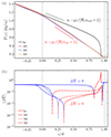 |
Fig. 1. Comparison of hydrostatic and convecting models. Panel a: Temperature as a function of height from a 1D hydrostatic model (black solid line) and convective runs A0 (red dashed line), A6 (blue dashed line), and A9 (orange dashed line). The black (red) dotted line shows a polytropic gradient corresponding to index nrad = 3.25 (nad = 1.5) for reference. Panel b: Absolute value of the superadiabatic temperature gradient Δ∇ from the same runs as indicated by the legend. Red (blue) indicates convectively unstable (stable) stratification. The dotted vertical lines at z = 0 and z/d = 1 denote the base and top of the initially isentropic layer. |
The horizontal boundaries are periodic, and the vertical boundaries are impenetrable and stress free according to
 (10)
(10)
A constant energy flux is imposed at the lower boundary by setting
 (11)
(11)
where Fbot is the fixed input flux and Kbot = K(x, y, zbot). A constant temperature T = Ttop is imposed on the upper vertical boundary.
2.2. Units and control parameters
The units of length, time, density, and entropy are given by
![Mathematical equation: $$ \begin{aligned}[x] = d,\ \ \ [t] = \sqrt{d/g},\ \ \ [\rho ] = \rho _0,\ \ \ [s] = c_{\rm P}, \end{aligned} $$](/articles/aa/full_html/2024/03/aa48325-23/aa48325-23-eq16.gif) (12)
(12)
where ρ0 is the initial value of density at z = ztop. The models are fully defined by choosing the values of ν, Ω0, θ, g, a, b, K0, ρ0, T0, τcool, and the SGS Prandtl number
 (13)
(13)
along with the cooling profile fcool(z). The values of K0, ρ0, T0 are subsumed into another constant  , which is fixed by assuming the radiative flux at zbot to equal Fbot at t = 0. The cooling profile fcool(z)=1 above z/d = 1 and fcool(z)=0 below z/d = 1, connecting smoothly across the interface over a width of 0.025d. The quantity
  sets the initial pressure scale height at the surface and determines the initial density stratification. All of the current simulations have ξ0 = 0.054.
The Prandtl number based on the radiative heat conductivity is
 (14)
(14)
where χ(x)=K(x)/cPρ(x) quantifies the relative importance of viscous to temperature diffusion. Unlike many other simulations, Pr is not an input parameter because of the non-linear dependence of the radiative diffusivity on the ambient thermodynamics. The dimensionless normalised flux is given by
 (15)
(15)
where ρ(zbot) and cs(zbot) are the density and the sound speed, respectively, at z = zbot at t = 0. At the base of the solar CZ ℱn ≈ 4 × 10⁻¹¹ (e.g., Brandenburg et al. 2005), whereas in the current fully compressible simulations, several orders of magnitude larger values are used (see Table 1).
Summary of the runs.
The effect of rotation is quantified by the Taylor number
 (16)
(16)
which is related to the Ekman number via Ek = Ta−1/2.
The Rayleigh number based on the energy flux is given by
 (17)
(17)
This can be used to construct a flux-based diffusion-free modified Rayleigh number (e.g., Christensen 2002; Christensen & Aubert 2006)
 (18)
(18)
In the current setup,  is given by
 (19)
(19)
A reference depth needs to be chosen because  . Furthermore, H ≡ cPT/g is a length scale related to the pressure scale height. The choice d = H = Hp, where Hp ≡ −(∂lnp/∂z)−1 is the pressure scale height at the base of the convection zone, leads to
 (20)
(20)
2.3. Diagnostics quantities
The global Reynolds and SGS Péclet numbers describe the strength of advection versus viscosity and SGS diffusion
 (21)
(21)
where urms is the volume-averaged rms velocity and where k1 = 2π/d is an estimate of the largest eddies in the system. The Reynolds and Péclet number based on the actual convective length scale ℓ are given by
 (22)
(22)
Here,  is chosen, where kmean = kmean(z) is the mean wavenumber (e.g., Christensen & Aubert 2006; Schrinner et al. 2012) and is computed from
 (23)
(23)
where E(k, z) is the power spectrum of the velocity field with u2(z)=∫E(k, z)dk.
In general, the total thermal diffusivity is given by
 (24)
(24)
However, in all of the current simulations, χ ≪ χSGS in the CZ such that the Prandtl and Péclet numbers based on χeff differ little from PrSGS and PeSGS. The Rayleigh number is defined as
 (25)
(25)
which varies as a function of height and is quoted near the surface at z/d = 0.85. The Rayleigh number in the hydrostatic, non-convecting, state is measured from a one-dimensional model that was run to thermal equilibrium and where the convectively unstable layer is confined to the near-surface layers (Brandenburg 2016); see also Fig. 1. In the hydrostatic case, χ = χ(z), and χSGS, which affects only the fluctuations, plays no role. The turbulent Rayleigh number is quoted from the statistically stationary state using the horizontally averaged mean state,
 (26)
(26)
where the overbar denotes temporal and horizontal averaging.
The rotational influence on the flow is measured by several versions of the Coriolis number. First, the global Coriolis number is defined as
 (27)
(27)
where k1 = 2π/d is the wavenumber corresponding to the system scale. This definition neglects the changing length scale as a function of rotation and overestimates the rotational influence when rotation is rapid and the convective scale is smaller. A definition that takes the changing length scale into account is given by the vorticity-based Coriolis number
 (28)
(28)
where ωrms is the volume-averaged rms value of the vorticity ω = ∇ × u. Another definition of the Coriolis number taking into account the changing length scale is given by
 (29)
(29)
where  where the overbar denotes averaging over time and CZ. This is a commonly used choice in simulations of convection in spherical shells (Schrinner et al. 2012; Gastine et al. 2014; see also Aurnou et al. 2020, who considered convection in the limits of slow rotation and rapid rotation).
We further define a flux Coriolis number CoF 2 as
 (30)
(30)
where u⋆ is a reference velocity obtained from
 (31)
(31)
where ρ⋆ is a reference density, taken here at the bottom of the CZ. The u⋆ does not, and does not need to, correspond to any actual velocity, and it rather represents the available energy flux. Therefore, CoF does not depend on any dynamical flow speed or length scale set by complicated interactions of convection, rotation, magnetism, or other relevant physics. On the other hand, CoF depends only on quantities that can either be measured (Ftot, Ω0) or deduced from stellar structure models with relatively little ambiguity (Hp, ρ⋆). The significance of CoF is seen when rearranging Eq. (20) to yield
 (32)
(32)
Identifying the lhs with  , Eq. (30), gives
 (33)
(33)
An often-used phrase in the context of convection simulations targeting the Sun is that while all the other system parameters are beyond the reach of current simulations, the rotational influence on the flow can be reproduced (e.g., Käpylä et al. 2023). Equation (33) gives this a more precise meaning in that the solar value of  needs to be matched by any simulation claiming to model the Sun.
The net vertical energy flux consists of contributions due to radiative diffusion, enthalpy flux, kinetic energy flux, and viscous flux, as well as the surface cooling:
 (34)
(34)
 (35)
(35)
 (36)
(36)
 (37)
(37)
 (38)
(38)
Here, the primes denote fluctuations and the overbars indicate horizontal averaging. The total convected flux (Cattaneo et al. 1991) is the sum of the enthalpy and kinetic energy fluxes:
 (39)
(39)
which corresponds to the convective flux in, for example, mixing length models of convection.
Another useful diagnostic is buoyancy, or Brunt-Väisälä frequency, which is given by
 (40)
(40)
and describes the stability of an atmosphere with respect to buoyancy fluctuations if N2 > 0. Finally, the Richardson number related to rotation in the stably stratified layers is defined as
 (41)
(41)
Averages denoted by overbars are typically taken over the horizontal directions and time, unless specifically stated otherwise.
3. Results
Three sets of simulations with varying ℱn and approximately the same values of CoF are presented in the current study. We refer to these as Sets A, B, and C. The non-rotating runs in these sets correspond respectively to Runs K3, K4, and K5 in Käpylä (2019) in terms of ℱn, although lower values of ν and χSGS were used in the runs of the present study. We note that when ℱn is varied between the sets of simulations, the rotation rate Ω0 and the diffusivities ν and χSGS are varied at the same time proportionally to  (see, e.g., Käpylä et al. 2020, and Appendix A for more details). Furthermore, the cooling time τcool is varied proportional to ℱn. The current simulations have modest Reynolds and Péclet numbers in comparison to astrophysically relevant parameter regimes (e.g., Ossendrijver 2003; Kupka & Muthsam 2017; Käpylä et al. 2023; see Table 1). Earlier studies from non-rotating convection suggest that results obtained at such modestly turbulent regimes remain robust also at the highest resolutions affordable (Käpylä 2021). This is due to the fact that the main energy transport mechanism (convection) and the main driver of convection (surface cooling) are not directly coupled to the diffusivities. However, the current cases with rotation are more complicated because the supercriticality of convection decreases with increasing rotation rate (e.g., Chandrasekhar 1961; Roberts 1968). The effects of decreasing supercriticality are not studied systematically here, but subsets of the runs in Set A were repeated with higher resolutions (5763 and 11523) and correspondingly higher RaF, Re, and Pe (see Sets Am and Ah in Table 1).
3.1. Hydrostatic solution
Earlier studies have shown that a purely radiative hydrostatic solution with the Kramers opacity law is a polytrope with index nrad = 3.25 (Barekat & Brandenburg 2014; Brandenburg 2016). Such a solution arises in the case where K = const. and ∇zT = const. To see if this configuration is recovered with the current setup, Eqs. (1) and (3) were solved numerically in a one-dimensional z-dependent model with otherwise the same parameters as in the 3D simulations corresponding to the runs in Set A. The resulting temperature profile is shown in Fig. 1a along with corresponding horizontally averaged profiles from convecting Runs A0, A6, and A9. The stratification is consistent with a polytrope corresponding to nrad up to a height of roughly z/d = 0.75. Near the nominal surface of the convection zone, z/d = 1, the temperature gradient steepens sharply because the cooling term relaxes the temperature toward a constant (z-independent) value near the surface. Therefore, neither K nor ∇zT are constants in this transition region between the radiative and the cooling layers. In the initial state the stratification is isothermal above z/d = 1, but because the cooling profile fcool has a finite width, cooling also occurs below z/d = 1, and the isothermal layer is wider in the final thermally saturated state. This also depends on the value of τcool. In the convective runs, the stratification is nearly piecewise polytropic, with index nrad near the base of the radiative layer and nearly isentropic with nad in the bulk of the CZ.
The superadiabatic temperature gradient is defined as
 (42)
(42)
where  is the logarithmic temperature gradient and ∇ad = 1 − 1/γ is the corresponding adiabatic gradient. Comparison of the hydrostatic profile and the non-rotating convective model A0 shows that the convectively unstable layer in the former is much thinner than in the latter. This is a direct consequence of the strong temperature and density dependence of the Kramers opacity law. A similar conclusion applies also to the Sun, where the hypothetical non-convecting hydrostatic equilibrium solution has a very thin superadiabatic layer (Brandenburg 2016). The steepness of the temperature gradient near the surface is characterised by the maximum value of (Δ∇)hyd, which is 23.4. By comparison, in the convective Run A0, max(Δ∇) = 0.12. The Rayleigh number, measured at z/d = 0.85, in the hydrostatic case is Ra = 5.4 × 10⁷, which is about an order of magnitude greater than Rat in Run A0.
3.2. Qualitative flow characteristic as a function of rotation
Figure 2 shows representative flow fields from runs with slow, intermediate, and rapid rotation corresponding to Coriolis numbers 0.13, 1.3, and 16.5, respectively. The effects of rotation are hardly discernible in the slowly rotating case A2, with Co = 0.13. In the run with intermediate rotation, Run A6 with Co = 1.3, the convection cells are somewhat smaller than in the slowly rotating case, and more vortical structures are visible near the surface. For the most rapidly rotating case, Run A9 with Co = 16.5, the size of the convection cells is drastically reduced in comparison to the other two runs, and clear alignment of the convection cells with the rotation vector can be seen. The simulations were run either from the initial conditions described in Sect. 2.1 or by continuing from snapshots of already thermally relaxed runs. In a few cases, both approaches were explored with the same system parameters. In all of these cases, the solutions converged to the same final state, suggesting independence from initial conditions.
 |
Fig. 2. Flow fields from Runs A2 with Co = 0.13 (left), A6 with Co = 1.3 (middle), and A9 Co = 16.5 (right) at the north pole (θ = 0°). The colours indicate vertical velocity, and the contours indicate streamlines. |
3.3. Convective scale as function of rotation
The power spectra E(k) of the velocity fields for the runs in Set A are shown in Fig. 3 from depths near the surface, at the middle, and near the base of the CZ. As was already evident from visual inspection of the flow fields, the dominant scale of the flow decreases as the rotation rate increases. Quantitatively, the wavenumber kmax, where E(k) has its maximum, increases roughly in proportion to Co1/2. The mean wavenumber kmean, computed from Eq. (23), shows the same scaling for Co ≳ 2. This is explained by the broader distribution of power at different wavenumbers at slow rotation in comparison to the rapid rotation cases where fewer, or just a single, convective modes are dominant (see Fig. 3).
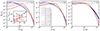 |
Fig. 3. Normalised velocity power spectra |
A decreasing length scale of the onset of linear instability under the influence of rotation was derived in Chandrasekhar (1961) with konset ∝ Ta2/3. With Ta ∝ Co2Re2 and with Re being approximately constant, konset ∝ Co1/3 is obtained. On the other hand, considering the CI part of the CIA balance in the Navier-Stokes equation gives (e.g,. Aurnou et al. 2020, see also Eq. (A.10)) gives
 (43)
(43)
or kmax ∝ Co1/2. This is consistent with the current simulations (see the inset in the left panel of Fig. 3). The same result was obtained in Featherstone & Hindman (2016). Some non-linear convection simulations show scalings that are similar but somewhat shallower than that obtained from the CIA balance (see, e.g., Viviani et al. 2018; Currie et al. 2020).
To estimate the convective length scale in the Sun based on the current results requires that the value of CoF matches that of the deep solar CZ. The quantities on the rhs of Eq. (30) at the base of the solar convection zone are Hp ≈ 5 × 10⁷ m, ρ⋆ ≈ 200 kg m−3,  kg s−3, with rCZ = 0.7 R⊙ ≈ 4.9 × 10⁸ m and L⊙ = 3.83 × 1026 W, and Ω⊙ = 2.7 × 10⁻⁶ s−1. Inserting this data into Eq. (30) yields
  . The values of CoF are listed for all runs in the ninth column of Table 1. The moderately rotating runs A5, B5, and C5 correspond to the rotational constraint at the base of the solar CZ with CoF = 3.0…3.2. The mean horizontal wavenumber kmean/kH ≈ 7, where kH = 2π/Lx, in these simulations corresponds to a horizontal scale of ℓconv = Lx(kH/kmean)≈0.57d. The pressure scale height at the base of the CZ is about 0.49d such that ℓconv ≈ 1.16Hp. Converting this to physical units using
  Mm yields ℓconv ≈ 58 Mm. Following the procedure of Featherstone & Hindman (2016) and using kmax instead of kmean, kmax/kH = 3, and ℓconv ≈ 130 Mm. Both of these estimates are significantly larger than the supergranular scale of 20…30 Mm, which was suggested to be the largest convectively driven scale in the Sun by Featherstone & Hindman (2016) and Vasil et al. (2021). On the other hand, a rapidly rotating run of Featherstone & Hindman (2016) with ℓconv ≈ 30 Mm had a Rossby number of
  , where
  is a typical velocity amplitude and H is the shell thickness. This corresponds to a global Coriolis number of
  in the conventions of the current study. In the current Runs A9, B9, and C9, Co ≈ 17 and kmax ≈ kmean ≈ 17, corresponding to ℓconv ≈ 26 Mm. Therefore, the current simulations give a very similar estimate for ℓconv as in Featherstone & Hindman (2016) at comparable values of Co despite the differences between the model setups. However, the values of CoF in Runs A9, B9, and C9 are at least 16 times higher than in the Sun, suggesting that the simulations of Featherstone & Hindman (2016) were also rotating much faster than the Sun3. Therefore, the current results suggest that rotationally constrained convection cannot explain the appearance of supergranular scale as the largest convective scale in the Sun.
Figure 4 shows the velocity power spectra for the most rapidly rotating runs with Co ≈ 17 for Re = 30…142 from Runs A9, A9m, and A9h. There is a marked increase in the power at large scales, which begins to affect kmean at the highest Re (run A9h). This is due to the gradual onset of large-scale vorticity production, most likely due to two-dimensionalisation of the turbulence, which has been observed in various earlier studies of rapidly rotating convection (e.g., Chan et al. 2003; Chan 2007; Chan & Mayr 2013; Käpylä et al. 2011; Guervilly et al. 2014). Despite the rapid rotation with Coriolis numbers exceeding 16, the large-scale vorticity generated in the current simulations is relatively modest, apart from run A9h. A difference from many of the previous studies is that here the relevant thermal Prandtl number (PrSGS) is on the order of unity, whereas in many of the earlier studies Pr was lower. Large-scale vorticity production was indeed observed in an additional run that is otherwise identical to A9 except that PrSGS = 0.2 instead of PrSGS = 1.
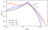 |
Fig. 4. Normalised velocity power spectra near the surface of simulations with Co ≈ 17 and Re = 30…142 (Runs A9, A9m, and A9h). The dotted line shows a Kolmogorov k−5/3 scaling for reference. |
3.4. Measures of rotational influence
3.4.1. Velocity-based Co
The suitability of different measures of rotational influence on the flow has been discussed in various works in the literature (e.g., Käpylä 2023b). A common (and justified) critique regarding the global Coriolis number as defined in Eq. (27) is that it does not appreciate the fact that ℓconv = ℓconv(Ω) (e.g., Vasil et al. 2021). The most straightforward way to correct this is to measure the mean wavenumber and use Eq. (29). Figure 5 shows Coℓ as a function of Co for all runs listed in Table 1. For slow rotation, Co ≲ 1, Coℓ ∝ Co because uconv and ℓconv are almost unaffected by rotation. For sufficiently rapid rotation this is no longer true because kmean ≈ kmax ∝ Co1/2, as indicated by Eq. (A.10) and the simulation results (see the inset of Fig. 3). This implies that for rapid rotation Coℓ ∝ Co1/2; see also Eq. (A.12). This is consistent with the numerical results found in the most rapidly rotating cases (see Fig. 5). The higher resolution runs in Set Am have somewhat lower Coℓ than the corresponding runs in Set A because the convective velocities in the higher resolution cases are higher. This shows that the simulations are not yet in an asymptotic regime where the results are independent of the diffusivities. This is further demonstrated by the high resolution runs of Set Ah. Run A5h follows the trend set by Run A5m. Run A9h, with a significantly higher Coℓ than in Runs A9 and A9m, is explained by the increasing kmean due to the large-scale vorticity generation in that case. Aurnou et al. (2020) showed that the dynamical Rossby number is related to the diffusion-free modified flux Rayleigh number  , with different powers for slow and rapid rotation. The corresponding derivations for the Coriolis number Coℓ are presented in Appendix A and show that
  (slow rotation) and
  (rapid rotation). Both scalings are also supported by the simulation results (see the inset of Fig. 5).
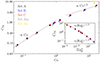 |
Fig. 5. Dynamical Coriolis number Coℓ as a function of Co for all of the runs in Table 1. Power laws proportional to Co (slow rotation; Co < 1) and Co1/2 (rapid rotation; Co > 2) are shown for reference. The inset shows Coℓ as a function of |


3.4.2. Vorticity-based Co
Another commonly used definition, Eq. (28), is used to take the changing length scale automatically into account. However, Coω comes with a caveat that has apparently not been discussed hitherto in the astrophysical literature. This is demonstrated by considering a set of rotating systems at asymptotically high Re where urms is independent of Re. The forcing is assumed fixed by a constant energy flux through the system and the asymptotic value of urms when Re → ∞ as u∞. Furthermore, in this regime the mean kinetic energy dissipation rate
 (44)
(44)
where the overbar denotes a suitably defined average, tends to a constant value when normalised by mean length and corresponding rms velocity (e.g., Sreenivasan 1984; Vassilicos 2015). This value is denoted as ϵ∞. In low-Mach number turbulence, which is a good approximation of stellar interiors, as well as the current simulations with Ma ∼ 𝒪(10−2),
 (45)
(45)
From the definition of system scale Reynolds number, it follows that
 (46)
(46)
and from Eq. (45) that
 (47)
(47)
Using Eq. (28), it is found that
 (48)
(48)
This means Coω → 0 as Re → ∞ at constant Co, while the dynamics at large (integral) scales are unaffected. Therefore Coω underestimates the rotational influence at the mean scale kmean that dominates the dynamics, as opposed to Eq. (27) overestimating it.
Equation (47) can also be written as
 (49)
(49)
For sufficiently large Re, the theoretical prediction is that urms → u∞ = const. and kω ∝ Re1/2. This has been confirmed from numerical simulations of isotropically forced homogeneous turbulence (e.g., Brandenburg & Petrosyan 2012; Candelaresi & Brandenburg 2013). We show the dependence of kω on Re in the inset of Fig. 6 for runs with Co ≈ 1.3 and Re ranging between 40 and 174. The results for kω fall somewhat below the theoretical Re1/2 expectation. This is likely because the asymptotic regime requires still higher Reynolds numbers. On the other hand, the mean wavenumber kmean is essentially constant around kmean/k1 = 7 in this range of Re because the dominating contribution to the velocity spectrum comes from large scales that are almost unaffected by the increase in Re.
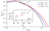 |
Fig. 6. Normalised velocity power spectra near the surface of simulations with Co ≈ 1.3 and Re = 40…174 (Runs A6, A6m, and A6h). The dotted line shows Kolmogorov k−5/3 scaling for reference. The inset shows |


3.5. Convective velocity as a function of total flux and rotation
The scalings of convective velocity as a function of rotation are derived in Appendix A following the same arguments as in Aurnou et al. (2020). For slow rotation, the convective velocity depends only on the energy flux
 (50)
(50)
where u⋆ is defined via Eq. (31). This scaling is altered in the rapidly rotating regime where
 (51)
(51)
This result agrees with Eq. (50d) of Aurnou et al. (2020) and Table 2 of Vasil et al. (2021). Therefore the velocity amplitude in the rapidly rotating regime is expected to depend not only on the available flux but also on rotation. Figure 7 shows the corresponding numerical results for the Sets A, B, C, and Am. For slow rotation, Co ≲ 1.5, urms is roughly constant around urms ≈ 1.15u⋆ for Sets A, B, and C and around urms ≈ 1.23u⋆ for Set Am. In the rapid rotation regime, urms follows a trend that is consistent to that indicated in Eq. (51), but the agreement is only obtained for the two highest values of Co. The higher resolution and more supercritical runs from Set Am show a similar trend, although the velocities are higher overall. This demonstrates that the current runs are not yet in an asymptotic regime where the effects of the diffusivities are negligible.
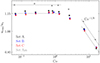 |
Fig. 7. Volume-averaged rms velocity normalised by u⋆ from Sets A, B, C, and Am. The dotted lines for Co < 1.5 denote constants 1.15 and 1.23, respectively, whereas for Co > 6, they are proportional to Co−1/6 as indicated by the theoretical CIA scaling (see Eq. (51)). |
3.6. Flow statistics
Compressible non-rotating convection is characterised by broad upflows and narrow downflows (Stein & Nordlund 1989; Cattaneo et al. 1991; see also Fig. 2). This can be described by the filling factor f of downflows as
![Mathematical equation: $$ \begin{aligned} \overline{u}_z(z) = f(z) \overline{u}_z^\downarrow + [1-f(z)] \overline{u}_z^\uparrow (z), \end{aligned} $$](/articles/aa/full_html/2024/03/aa48325-23/aa48325-23-eq88.gif) (52)
(52)
where  is the mean vertical velocity, whereas
  and
and  are the corresponding mean upflow and downflow velocities. It was shown in Käpylä (2021) that f is sensitive to the effective Prandtl number of the fluid such that a lower Pr leads to a lower filling factor. In the current paper we performed a similar study focusing on the function of rotation (see Fig. 8). The main result is that f approaches 1/2 in the rapid rotation regime. This is because in rapidly rotating convection, the broad upwellings of non-rotating convection are broken up and the flow consists mostly of smaller scale helical columns where the upflows and downflows are almost invariant. This is due to the Taylor–Proudmann constraint which causes derivatives along the rotation axis to vanish. Hence the tendency for larger structures to appear at greater depths is inhibited, and the average size of convection cells as a function of depth is almost constant (see rightmost panel of Fig. 2).
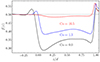 |
Fig. 8. Filling factor of downflows f(z) as a function of height for three runs with no (black; Run A0), moderate (blue; A6), and rapid (red; A9) rotation. |
This is also apparent from the probability density functions (PDFs) of the velocity components ui, defined via
 (53)
(53)
Figure 9 shows representative examples of PDFs for the extreme cases (Run A0 with Co = 0 and Run A9 with Co ≈ 16.5) and at an intermediate rotation rate (Run A6, Co = 1.3). In non-rotating convection, the PDFs of the horizontal components of the velocity are nearly Gaussian near the surface, whereas for uz the distributions are highly skewed due to the upflow and downflow asymmetry. In deeper parts, the horizontal velocities also deviate from a Gaussian distribution, in agreement with earlier works (e.g., Brandenburg et al. 1996; Hotta et al. 2015; Käpylä 2021).
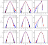 |
Fig. 9. Probability density functions 𝒫(ui) for ux (left), uy (middle), and uz (right) for depths z/d = 0.85 (black), z/d = 0.49 (blue), and z/d = 0.13 (red) for runs with Co = 0 (Run A0, top row), Co = 1.3 (Run A6, middle), and Co = 16.5 (Run A9, bottom). The tildes refer to normalisation by the respective rms values. |
As the rotation increases, the asymmetry of the vertical velocity decreases such that in the most rapidly rotating cases considered in this work with Co ≈ 17, uz also approaches a Gaussian distribution. Only near the surface (z/d = 0.85) does a weak asymmetry remain. The horizontal components of velocity continue to have a Gaussian distribution as rotation increases, although there is not enough data to say anything concrete concerning the tails of the distributions at high velocity amplitudes. To further quantify the statistics of the flow, skewness 𝒮 and kurtosis 𝒦 are computed from:
 (54)
(54)
where σu = (ℳ2)1/2, with
![Mathematical equation: $$ \begin{aligned} \mathcal{M} ^n(u_i,z) = \int [u_i(\boldsymbol{x}) - \overline{u}_i(z)]^n \mathcal{P} (u_i,z)\mathrm{d}u_i. \end{aligned} $$](/articles/aa/full_html/2024/03/aa48325-23/aa48325-23-eq94.gif) (55)
(55)
Figure 10 shows 𝒮 and 𝒦 for all ui for the same runs as in Fig. 9. The skewness is consistent with zero for the horizontal velocities, which is expected, as there is no anisotropy in the horizontal plane. The negative values of 𝒮 for uz are a signature of the asymmetry between upflows and downflows. As rotation increases, 𝒮 approaches zero also for uz. The kurtosis 𝒦 is a measure of non-Gaussianity, or intermittency. In the non-rotating case 𝒦 increases from roughly three, indicating Gaussian statistics, to roughly five for horizontal flows as a function of depth within the CZ. For uz, the increase of 𝒦 is much more dramatic below z/d ≲ 0.3. This is because downflows merge at deeper depths such that only a few of them survive deep in the CZ and especially in the overshoot region below roughly z = 0, where 𝒦 reaches a peak value of roughly 65 for Run A0. A similar, albeit lower, maximum also appears for the horizontal flows. At intermediate rotation (Run A6; Co = 1.3), uz still exhibits strong intermittency below z ≈ 0.1 with max(𝒦)≈54, whereas 𝒦 for the horizontal flows is significantly reduced in comparison to the non-rotating case. This indicates that the vertical flows in this regime especially are not qualitatively different from those in the non-rotating regime such that the downflows in the overshoot region are rather abruptly decelerated and diverted horizontally. For the most rapidly rotating case (Run A9; Co = 16.5), 𝒦 ≈ 3…4 throughout the simulation domain for both vertical and horizontal flows. This is explained by the almost complete wiping out of the upflow–downflow asymmetry also in the deep parts of the CZ and in the overshoot region. The absence of a peak in the kurtosis in the overshoot region in the most rapidly rotating cases is likely due to the deeply penetrating vertical flows in those cases due to the unrealistically small Richardson number. This is discussed in more detail in Sect. 3.7.
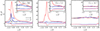 |
Fig. 10. Skewness (𝒮, dashed lines) and kurtosis (𝒦, solid) from the same runs as in Fig. 9. The black, blue, and red colours indicate data corresponding to ux, uy, and uz, respectively. We note the difference in scale between each of the panels. The insets show a zoom-in of the region z/d ≥ 0. |
The average vertical rms velocities from the same runs as in Fig. 9 are shown in Fig. 11. The average rms velocity of the downflows (upflows) is always larger (smaller) than the average total vertical rms velocity. However, the difference between the upflows and downflows and the total rms velocity diminishes monotonically as a function of rotation such that for the most rapidly rotating case the three are almost the same. This is another manifestation of the symmetrisation of upflows and downflows.
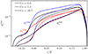 |
Fig. 11. Horizontally averaged vertical rms velocity for the same runs as in Fig. 9. The overall vertical velocity ( |


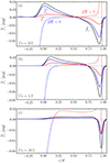 |
Fig. 12. Horizontally averaged total force (black) and the force acting on upflows (red) and downflows (blue). The dotted red and blue lines show the superadiabatic temperature gradient. Data are shown for (a) a non-rotating Run A0, (b) an intermediate rotation rate (Co = 1.3, Run A6), and (c) for rapid rotation (Co = 16.5, Run A9). |
Another consequence of the symmetrisation of the vertical flows is that the forces on the upflows and downflows also approach each other (see Fig. 12), where  . In accordance with earlier studies (Käpylä et al. 2017; Käpylä 2019), in non-rotating convection, the downflows are accelerated near the surface and decelerated roughly when the stratification turns Schwarzschild stable, whereas the upflows are accelerated everywhere except near the surface. This is interpreted such that the upflows are not driven by buoyancy but by pressure forces due to the deeply penetrating downflow plumes. This qualitative picture remains unchanged for slow and intermediate rotation (see Fig. 12b). For rapid rotation, the forces on the upflows and downflows are nearly identical. However, the situation continues to qualitatively deviate from the mixing length picture also in the rapidly rotating cases in that the downflows are accelerated only near the surface and braked throughout their descent through the superadiabatic CZ (see Fig. 12c).
3.7. Overshooting and Deardorff zones
We studied the depths of the overshooting and Deardorff zones as functions of rotation using the same definitions as in previous studies (Käpylä 2019, 2021). We defined the bottom of the CZ to be the depth zCZ where  changes from negative to positive with increasing z. The top of the Deardorff zone (DZ) – or the bottom of the buoyancy zone (BZ) – zBZ was taken to be where the superadiabatic temperature gradient changes from negative to positive with increasing z. The depth of the DZ is then
![Mathematical equation: $$ \begin{aligned} d_{\rm DZ} = \frac{1}{\Delta t} \int _{t_0}^{t_1} [z_{\rm BZ}(t)-z_{\rm CZ}(t)]\mathrm{d}t, \end{aligned} $$](/articles/aa/full_html/2024/03/aa48325-23/aa48325-23-eq101.gif) (56)
(56)
where Δt = t1 − t0 is the length of the statistically steady part of the time series. We measured a reference value of the kinetic energy flux ( ) at zCZ. The base of the overshoot zone (OZ) is taken to be the location (
 ) where
  falls below
  and
and
![Mathematical equation: $$ \begin{aligned} d_{\rm OZ}^\mathrm{kin} = \frac{1}{\Delta t} \int _{t_0}^{t_1} [z_{\rm CZ}(t)-z_{\rm OZ}^\mathrm{kin}(t)]\mathrm{d}t. \end{aligned} $$](/articles/aa/full_html/2024/03/aa48325-23/aa48325-23-eq106.gif) (57)
(57)
This criterion breaks down in the current models when rotation begins to dominate the dynamics and where  . Therefore, the convected flux
  was also used to estimate the depth of overshooting. The criterion involving
  assumes the overshoot zone ends at the location (
 ) where
  falls below 0.02Ftot. We computed the corresponding overshooting depth (
 ) analogously to Eq. (57). The layer below the OZ is the radiative zone (RZ).
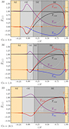 |
Fig. 13. Time-averaged mean energy fluxes as defined in Eqs. (34) and (38) (apart from the negligibly small viscous flux |

Figure 13 shows the energy fluxes from representative runs at different Coriolis numbers from Set A. For slow and moderate rotation up to Co ≈ 1, the situation is qualitatively similar: the positive (upward) enthalpy flux exceeds Fbot in the bulk of the CZ, and it is compensated by a negative (downward) kinetic energy flux  . As rotation increases, the maxima of
  and
and  decrease monotonically. Similarly, the extents of the overshoot and Deardorff zones diminish with rotation. For the case with the most rapid rotation, Run A9 with Co = 16.5, the kinetic energy flux is almost zero, and
  . This is yet another manifestation of the decreasing asymmetry between the upflows and downflows. Moreover, the Deardorff zone vanishes in the rapidly rotating cases.
Summary of the buoyancy, Deardorff, and overshoot zones.
The positions of the boundaries of the different layers and their depths are summarised for all runs in Table 2, and Fig. 14 shows a summary of the overshooting and Deardorff zone depths as a function of rotation from Sets A, B, and C. The main difference between the sets of simulations is the applied flux ℱn. The overshooting depth measured from the kinetic energy flux decreases with increasing rotation as in earlier studies (e.g., Ziegler & Rüdiger 2003; Käpylä et al. 2004). However, the lowermost panel of Fig. 13 shows that the upper part of the radiative zone is mixed far beyond the regions where  is non-negligible in the rapidly rotating cases. This is confirmed when the convected flux is used to estimate the overshooting depth. Furthermore,
  increases with rotation for Co ≳ 1. This is explained by the fact that the Mach number, and therefore also the rotation rate Ω0, in the current simulations are much larger than in real stars. This means that the convective, rotation, and Brunt-Väisälä frequencies are closer to each other in the simulations in comparison to the overshoot region of the Sun. For example, in the most rapidly rotating runs, the Richardson number RiΩ based on the rotation rate is smaller than unity (see the 12th panel of Table 1). This, in addition to the smooth transition from the convective to the radiative region, can lead to gravity waves breaking in the radiative zone, thus contributing to the burrowing of the flows into the RZ (e.g., Lecoanet & Quataert 2013). As a comparison, RiΩ in the upper part of the solar radiative zone is expected to be on the order of 104. Another possibility is that shear caused by the rotationally constrained convective columns lowers the corresponding shear Richardson number close to the limit where turbulence can occur also in stable stratification.
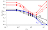 |
Fig. 14. Depth of the overshoot zone from kinetic energy ( |


Lowering the luminosity in Sets B and C shows that both measures of dOZ decrease with ℱn in qualitative accordance with earlier results (e.g., Käpylä 2019). Even though RiΩ modestly increases in these runs (see the 12th column in Table 1), the most rapidly rotating cases, even in the runs with the lowest luminosities, continue to show deep mixing, which is most likely due to the still unrealistically low RiΩ. It is numerically very expensive to increase the Richardson number in fully compressible simulations much further, at least without accelerated thermal evolution methods (e.g., Anders et al. 2018, 2020). Comparing the overshooting depths between Runs [A,B,C]5 with solar CoF and the non-rotating Runs [A,B,C]0 shows a reduction between about a third to a half (see the seventh and eight columns in Table 2). In Käpylä (2019) the overshooting depth extrapolated to the solar value of ℱn was found to be roughly 0.1Hp, and the current results including rotation reduce this to 0.05…0.07Hp. However, the dependence of the overshooting depth on ℱn is steeper here (![Mathematical equation: $ [\tilde{d}_{\mathrm{OZ}}^{\mathrm{kin}},\tilde{d}_{\mathrm{OZ}}^{\mathrm{conv}}] \propto {\mathscr{F}}_{\mathrm{n}}^{0.15} $](/articles/aa/full_html/2024/03/aa48325-23/aa48325-23-eq126.gif) ) than in the nonrotating cases where Käpylä (2019) found
) than in the nonrotating cases where Käpylä (2019) found  .
.
On the other hand, the thickness of the Deardorff zone dDZ decreases monotonously as a function of Co. In the most rapidly rotating cases, the Deardorff zone vanishes altogether and even reverses such that at the base of the CZ, the stratification is unstably stratified but the convective flux is inward (see the lowermost panel of Fig. 13). This does not change significantly in more supercritical runs, such as A9m and A9h. In the entropy rain picture (e.g., Brandenburg 2016), cool material from the surface is brought down deep into the otherwise stably stratified layers. This is mediated by relatively few fast downflows with a filling factor of f(z)< 1/2 that also produce a strong net downward kinetic energy flux, as seen in the top panel of Fig. 13 (see also Fig. 8 and Table 1 and Sect. 3.3 in Brandenburg 2016). If, on the other hand, the upflows and downflows are symmetrised such that f(z)=1/2 and their velocities are nearly the same,  vanishes, and non-local transport due to downflows is no longer significant. Therefore, the kinetic energy flux is a proxy of the non-local transport due to downflows, and its absence signifies the absence of a Deardorff zone. The depth of the Deardorff zone is independent of the energy flux ℱn. This further illustrates that the DZ is caused by surface effects that are kept independent of ℱn in the current simulations. A reduction of dDZ of about a third between the non-rotating runs [A,B,C]0 and the runs with the solar value of CoF (Runs [A,B,C]5) was found (see the sixth column of Table 2).
4. Conclusions
Simulations of compressible convection were used to study the convective scale and scalings of quantitites such as the Coriolis number and convective velocity as functions of rotation. The results were compared to those expected from scalings obtained for incompressible convection with slow and fast rotation (Aurnou et al. 2020). The actual length scale is almost unaffected by rotation for Co ≲ 1 and decreases proportionally to Co1/2 for rapid rotation. Correspondingly, the dynamical Coriolis number Coℓ is proportional to Co for slow rotation and to ∝Co1/2 for rapid rotation. Furthermore, Coℓ is proportional to  for slow and
  for rapid rotation, where
  is the diffusion-free flux-based modified Rayleigh number. Finally, the convective velocity is compatible with proportionality to (Ftot/ρ)1/3 for slow and ∝(Ftot/ρ)1/3Co−1/6 for rapid rotation. All of these scalings are consistent with those derived by Aurnou et al. (2020) and Vasil et al. (2021).
In an earlier work (Käpylä 2023b), several measures were used to characterise the rotational influence on convection. A commonly used definition where the changing length scale of convection is taken into account is Coω = 2Ω/ωrms. We have shown that this quantity cannot be used to characterise the effects of rotation on the mean scale because ωrms is expected to increase with the Reynolds number as Re1/2. Therefore the only reliable way to account for the changing convective length scale as a function of rotation is to compute the mean wavenumber. This was not correctly identified in Käpylä (2023b), and it is now clear that Coω will diverge as Re increases. On the other hand, Käpylä (2023b) introduced a stellar Coriolis number Co⋆ that depends on luminosity and rotation rate, which are observable, and a reference density, which is available from stellar structure models, but not on any dynamical length or velocity scale. In our work, we renamed this quantity as CoF, and we showed that with a suitable choice of length scale,  . Matching CoF (or equivalently
  ) with the target star gives more concrete meaning to the often-expressed idea that it is possible to match the Coriolis number of, for example, the Sun with 3D simulations, while most other dimensionless parameters are out of reach (cf. Käpylä et al. 2023).
The current simulations suggest that convection, even in the deep parts of the CZ in the Sun, is not strongly rotationally constrained and that the CIA balance is therefore inapplicable there. The latter has been assumed to be the case by Featherstone & Hindman (2016) and Vasil et al. (2021) to argue that the largest convectively driven scale in the Sun is the supergranular scale. The current results seem to refute this conjecture and we instead argue that the actual scales may be larger.
Finally, the effects of rotation on convective overshooting and subadiabatic Deardorff zones were studied. The effects of rotation are relatively mild such that for the case with the solar value of CoF, the overshooting depth and the extent of the Deardorff zone are reduced by between 30% and 50% in comparison to the non-rotating case. Therefore the current results suggest an overshooting depth of about 5% of the pressure scale height at the base of the solar CZ. Taking the current results at face value, a similar depth is estimated for the Deardorf zone. However, the latter is still subject to the caveat that the current simulations do not capture the near-surface layer very accurately (e.g., Käpylä 2023a) and that the driving of entropy rain can be significantly stronger in reality. Another aspect that needs to be revisited in the future is the effect of magnetic fields.
The same quantity was referred to as stellar Coriolis number in Käpylä (2023b).
For example, their run with Ro = 0.011 has RaF = 6.81 × 10⁶, Ek = 1.91 × 10⁻⁴, and Pr = 1, and corresponds to  , or
, or  . We note that here Ek = 2Ta−1/2. This yields
 ![Mathematical equation: $ \Omega/\Omega_\odot \approx [({\rm Ra}_{\rm F}^\star)_\odot/{\rm Ra}_{\rm F}^\star]^{1/3}\approx 17.6 $](/articles/aa/full_html/2024/03/aa48325-23/aa48325-23-eq136.gif) , which is approximate because somewhat different length scales were used.
, which is approximate because somewhat different length scales were used.
Acknowledgments
I thank Axel Brandenburg, Jose Fuentes Baeza, and Kishore Gopalakrishnan for their comments on an earlier version of the manuscript. The simulations were performed using the resources granted by the Gauss Center for Supercomputing for the Large-Scale computing project “Cracking the Convective Conundrum” in the Leibniz Supercomputing Centre’s SuperMUC-NG supercomputer in Garching, Germany. This work was supported in part by the Deutsche Forschungsgemeinschaft (DFG, German Research Foundation) Heisenberg programme (grant No. KA 4825/4-1), and by the Munich Institute for Astro-, Particle and BioPhysics (MIAPbP) which is funded by the DFG under Germany’s Excellence Strategy – EXC-2094 – 390783311.
References
- Anders, E. H., & Pedersen, M. G. 2023, Galaxies, 11, 56 [NASA ADS] [CrossRef] [Google Scholar]
- Anders, E. H., Brown, B. P., & Oishi, J. S. 2018, Phys. Rev. Fluids, 3, 083502 [NASA ADS] [CrossRef] [Google Scholar]
- Anders, E. H., Vasil, G. M., Brown, B. P., & Korre, L. 2020, Phys. Rev. Fluids, 5, 083501 [NASA ADS] [CrossRef] [Google Scholar]
- Anders, E. H., Jermyn, A. S., Lecoanet, D., & Brown, B. P. 2022, ApJ, 926, 169 [NASA ADS] [CrossRef] [Google Scholar]
- Aurnou, J. M., Horn, S., & Julien, K. 2020, Phys. Rev. Res., 2, 043115 [NASA ADS] [CrossRef] [Google Scholar]
- Barekat, A., & Brandenburg, A. 2014, A&A, 571, A68 [NASA ADS] [CrossRef] [EDP Sciences] [Google Scholar]
- Barker, A. J., Dempsey, A. M., & Lithwick, Y. 2014, ApJ, 791, 13 [Google Scholar]
- Bekki, Y., Hotta, H., & Yokoyama, T. 2017, ApJ, 851, 74 [NASA ADS] [CrossRef] [Google Scholar]
- Böhm-Vitense, E. 1958, ZAp, 46, 108 [NASA ADS] [Google Scholar]
- Brandenburg, A. 2016, ApJ, 832, 6 [Google Scholar]
- Brandenburg, A., & Petrosyan, A. 2012, Astron. Nachr., 333, 195 [NASA ADS] [CrossRef] [Google Scholar]
- Brandenburg, A., Jennings, R. L., Nordlund, Å., et al. 1996, J. Fluid Mech., 306, 325 [NASA ADS] [CrossRef] [Google Scholar]
- Brandenburg, A., Nordlund, A., & Stein, R. F. 2000, in Geophysical and Astrophysical Convection, Contributions from a workshop sponsored by the Geophysical Turbulence Program at the National Center for Atmospheric Research, October 1995, eds. P. A. Fox, & R. M. Kerr (The Netherlands: Gordon and Breach Science Publishers), 85 [Google Scholar]
- Brandenburg, A., Chan, K. L., Nordlund, Å., & Stein, R. F. 2005, Astron. Nachr., 326, 681 [NASA ADS] [CrossRef] [Google Scholar]
- Brummell, N. H., Clune, T. L., & Toomre, J. 2002, ApJ, 570, 825 [NASA ADS] [CrossRef] [Google Scholar]
- Brun, A. S., Strugarek, A., Varela, J., et al. 2017, ApJ, 836, 192 [Google Scholar]
- Candelaresi, S., & Brandenburg, A. 2013, Phys. Rev. E, 87, 043104P [NASA ADS] [CrossRef] [Google Scholar]
- Cattaneo, F., Brummell, N. H., Toomre, J., Malagoli, A., & Hurlburt, N. E. 1991, ApJ, 370, 282 [CrossRef] [Google Scholar]
- Chan, K. L. 2003, in 3D Stellar Evolution, eds. S. Turcotte, S. C. Keller, & R. M. Cavallo, ASP Conf. Ser., 293, 168 [NASA ADS] [Google Scholar]
- Chan, K. L. 2007, Astron. Nachr., 328, 1059 [NASA ADS] [CrossRef] [Google Scholar]
- Chan, K. L., & Mayr, H. G. 2013, Earth Planet. Sci. Lett., 371, 212 [CrossRef] [Google Scholar]
- Chandrasekhar, S. 1961, Hydrodynamic and Hydromagnetic Stability (Oxford: Clarendon) [Google Scholar]
- Christensen, U. R. 2002, J. Fluid Mech., 470, 115 [NASA ADS] [CrossRef] [Google Scholar]
- Christensen, U. R., & Aubert, J. 2006, Geophys. J. Int., 166, 97 [NASA ADS] [CrossRef] [Google Scholar]
- Currie, L. K., Barker, A. J., Lithwick, Y., & Browning, M. K. 2020, MNRAS, 493, 5233 [CrossRef] [Google Scholar]
- Deardorff, J. W. 1961, J. Atmosph. Sci., 18, 540 [NASA ADS] [Google Scholar]
- Deardorff, J. W. 1966, J. Atmosph. Sci., 23, 503 [NASA ADS] [CrossRef] [Google Scholar]
- Dobler, W., Stix, M., & Brandenburg, A. 2006, ApJ, 638, 336 [NASA ADS] [CrossRef] [Google Scholar]
- Edwards, J. M. 1990, MNRAS, 242, 224 [NASA ADS] [CrossRef] [Google Scholar]
- Featherstone, N. A., & Hindman, B. W. 2016, ApJ, 830, L15 [Google Scholar]
- Fuentes, J. R., Anders, E. H., Cumming, A., & Hindman, B. W. 2023, ApJ, 950, L4 [NASA ADS] [CrossRef] [Google Scholar]
- Gastine, T., Yadav, R. K., Morin, J., Reiners, A., & Wicht, J. 2014, MNRAS, 438, L76 [CrossRef] [Google Scholar]
- Greer, B. J., Hindman, B. W., Featherstone, N. A., & Toomre, J. 2015, ApJ, 803, L17 [Google Scholar]
- Guervilly, C., Hughes, D. W., & Jones, C. A. 2014, J. Fluid Mech., 758, 407 [NASA ADS] [CrossRef] [Google Scholar]
- Hanasoge, S. M., Duvall, T. L., & Sreenivasan, K. R. 2012, Proc. Natl. Acad. Sci., 109, 11928 [Google Scholar]
- Hanasoge, S., Gizon, L., & Sreenivasan, K. R. 2016, Ann. Rev. Fluid Mech., 48, 191 [Google Scholar]
- Hotta, H. 2017, ApJ, 843, 52 [Google Scholar]
- Hotta, H., Rempel, M., & Yokoyama, T. 2015, ApJ, 803, 42 [NASA ADS] [CrossRef] [Google Scholar]
- Ingersoll, A. P., & Pollard, D. 1982, Icarus, 52, 62 [NASA ADS] [CrossRef] [Google Scholar]
- Käpylä, P. J. 2019, A&A, 631, A122 [NASA ADS] [CrossRef] [EDP Sciences] [Google Scholar]
- Käpylä, P. J. 2021, A&A, 655, A78 [NASA ADS] [CrossRef] [EDP Sciences] [Google Scholar]
- Käpylä, P. J. 2023a, arXiv e-prints [arXiv:2311.09082] [Google Scholar]
- Käpylä, P. J. 2023b, A&A, 669, A98 [NASA ADS] [CrossRef] [EDP Sciences] [Google Scholar]
- Käpylä, P. J., Korpi, M. J., & Tuominen, I. 2004, A&A, 422, 793 [NASA ADS] [CrossRef] [EDP Sciences] [Google Scholar]
- Käpylä, P. J., Mantere, M. J., & Hackman, T. 2011, ApJ, 742, 34 [CrossRef] [Google Scholar]
- Käpylä, P. J., Rheinhardt, M., Brandenburg, A., et al. 2017, ApJ, 845, L23 [CrossRef] [Google Scholar]
- Käpylä, P. J., Viviani, M., Käpylä, M. J., Brandenburg, A., & Spada, F. 2019, Geophys. Astrophys. Fluid Dyn., 113, 149 [CrossRef] [Google Scholar]
- Käpylä, P. J., Gent, F. A., Olspert, N., Käpylä, M. J., & Brandenburg, A. 2020, Geophys. Astrophys. Fluid Dyn., 114, 8 [CrossRef] [Google Scholar]
- Käpylä, P. J., Browning, M. K., Brun, A. S., Guerrero, G., & Warnecke, J. 2023, Space Sci. Rev., 219, 58 [CrossRef] [Google Scholar]
- Karak, B. B., Miesch, M., & Bekki, Y. 2018, Phys. Fluids, 30, 046602P [NASA ADS] [CrossRef] [Google Scholar]
- King, E. M., & Buffett, B. A. 2013, Earth Planet. Sci. Lett., 371, 156 [CrossRef] [Google Scholar]
- Kupka, F., & Muthsam, H. J. 2017, Liv. Rev. Comp. Astrophys., 3, 1 [NASA ADS] [CrossRef] [Google Scholar]
- Lecoanet, D., & Quataert, E. 2013, MNRAS, 430, 2363 [Google Scholar]
- O’Mara, B., Miesch, M. S., Featherstone, N. A., & Augustson, K. C. 2016, Adv. Space Res., 58, 1475 [CrossRef] [Google Scholar]
- Ossendrijver, M. 2003, A&ARv, 11, 287 [Google Scholar]
- Pencil Code Collaboration (Brandenburg, A., et al.) 2021, J. Open Source Softw., 6, 2807 [Google Scholar]
- Proxauf, B. 2021, PhD Thesis, Georg August University of Göttingen, Germany [Google Scholar]
- Roberts, P. H. 1968, Phil. Trans. Royal Soc. London Ser. A, 263, 93 [NASA ADS] [CrossRef] [Google Scholar]
- Roxburgh, L. W., & Simmons, J. 1993, A&A, 277, 93 [NASA ADS] [Google Scholar]
- Saikia, E., Singh, H. P., Chan, K. L., Roxburgh, I. W., & Srivastava, M. P. 2000, ApJ, 529, 402 [NASA ADS] [CrossRef] [Google Scholar]
- Schrinner, M., Petitdemange, L., & Dormy, E. 2012, ApJ, 752, 121 [NASA ADS] [CrossRef] [Google Scholar]
- Schumacher, J., & Sreenivasan, K. R. 2020, Rev. Mod. Phys., 92, 041001 [NASA ADS] [CrossRef] [Google Scholar]
- Singh, H. P., Roxburgh, I. W., & Chan, K. L. 1995, A&A, 295, 703 [NASA ADS] [Google Scholar]
- Singh, H. P., Roxburgh, I. W., & Chan, K. L. 1998, A&A, 340, 178 [NASA ADS] [Google Scholar]
- Spruit, H. 1997, Mem. Soc. Astron. Ital., 68, 397 [NASA ADS] [Google Scholar]
- Sreenivasan, K. R. 1984, Phys. Fluids, 27, 1048 [NASA ADS] [CrossRef] [Google Scholar]
- Stein, R. F., & Nordlund, Å. 1989, ApJ, 342, L95 [Google Scholar]
- Stein, R. F., & Nordlund, Å. 1998, ApJ, 499, 914 [Google Scholar]
- Stevenson, D. J. 1979, Geophys. Astrophys. Fluid Dyn., 12, 139 [NASA ADS] [CrossRef] [Google Scholar]
- Tremblay, P.-E., Ludwig, H.-G., Freytag, B., et al. 2015, ApJ, 799, 142 [Google Scholar]
- Vasil, G. M., Julien, K., & Featherstone, N. A. 2021, Proc. Natl. Acad. Sci., 118 [CrossRef] [Google Scholar]
- Vassilicos, J. C. 2015, Ann. Rev. Fluid Mech., 47, 95 [NASA ADS] [CrossRef] [Google Scholar]
- Vitense, E. 1953, ZAp, 32, 135 [Google Scholar]
- Viviani, M., & Käpylä, M. J. 2021, A&A, 645, A141 [EDP Sciences] [Google Scholar]
- Viviani, M., Warnecke, J., Käpylä, M. J., et al. 2018, A&A, 616, A160 [NASA ADS] [CrossRef] [EDP Sciences] [Google Scholar]
- Weiss, A., Hillebrandt, W., Thomas, H.-C., & Ritter, H. 2004, Cox and Giuli’s Principles of Stellar Structure (Cambridge: Cambridge Scientific Publishers Ltd) [Google Scholar]
- Ziegler, U., & Rüdiger, G. 2003, A&A, 401, 433 [EDP Sciences] [Google Scholar]
Appendix A: Convective scalings as function of rotation
The scalings of relevant dynamical quantities in convection are shortly summarised following the studies of Barker et al. (2014), Aurnou et al. (2020), and Vasil et al. (2021). In the rapidly rotating regime, the Coriolis-inertial-Archimedean (CIA) balance is assumed to hold.
A.1. No or slow rotation (Co ≪ 1)
For slow rotation, the convective length scale ℓconv is on the order of the pressure scale height Hp = −(∂lnp/∂z)−1, and the vertical and horizontal extents of convection cells are of the same order of magnitude. When rotation is slow, the dominant balance in the Navier–Stokes equation is between the advection and buoyancy terms:
 (A.1)
(A.1)
where H is the convective scale and T′ is the temperature fluctuation. Assuming that convection transports most of the energy gives
 (A.2)
(A.2)
and therefore,
 (A.3)
(A.3)
Choosing H = cPT/g gives
 (A.4)
(A.4)
where u⋆ is a hypothetical velocity that is a measure of the available energy flux. Therefore, for slow rotation,
 (A.5)
(A.5)
Temperature fluctuation can be computed from the convective flux
 (A.6)
(A.6)
Using u from Eq. (A.4) yields
 (A.7)
(A.7)
A.2. Rapid rotation (Co ≫ 1)
The CIA balance means that
 (A.8)
(A.8)
which results from the curl of the Navier–Stokes equation (e.g. Aurnou et al. 2020) and where ∂∥ is a derivative along the rotation vector. Considering first the CI part of the CIA balance gives
 (A.9)
(A.9)
where k⊥ and k∥ are the wavenumbers perpendicular and parallel to the rotation vector. Identifying k⊥ as the dominant horizontal scale of convection (kmax ∼ ℓ−1) and k∥ as k1 ∼ H−1 leads to
 (A.10)
Furthermore,
 (A.11)
or
 (A.12)
The convective length scale in terms of u and global quantities is
 (A.13)
To derive the convective velocity, the CA part of the CIA balance is used:
 (A.14)
Substituting ℓ from Eq. (A.13) and rearranging yields
 (A.15)
where H = cPT/g is used. This is equivalent to
 (A.16)
The length scale ℓ is obtained from Eq. (A.14) with the substitution of u from Eq. (A.15)
 (A.17)
where H = cPT/g is again used. Now,
 (A.18)
Bearing Eq. (20) in mind gives
 (A.19)
Finally, the temperature fluctuation using Eq. (A.16) is
 (A.20)
All Tables
All Figures
|
Fig. 1. Comparison of hydrostatic and convecting models. Panel a: Temperature as a function of height from a 1D hydrostatic model (black solid line) and convective runs A0 (red dashed line), A6 (blue dashed line), and A9 (orange dashed line). The black (red) dotted line shows a polytropic gradient corresponding to index nrad = 3.25 (nad = 1.5) for reference. Panel b: Absolute value of the superadiabatic temperature gradient Δ∇ from the same runs as indicated by the legend. Red (blue) indicates convectively unstable (stable) stratification. The dotted vertical lines at z = 0 and z/d = 1 denote the base and top of the initially isentropic layer. |
| In the text | |
|
Fig. 2. Flow fields from Runs A2 with Co = 0.13 (left), A6 with Co = 1.3 (middle), and A9 Co = 16.5 (right) at the north pole (θ = 0°). The colours indicate vertical velocity, and the contours indicate streamlines. |
| In the text | |
|
Fig. 3. Normalised velocity power spectra |
| In the text | |
|
Fig. 4. Normalised velocity power spectra near the surface of simulations with Co ≈ 17 and Re = 30…142 (Runs A9, A9m, and A9h). The dotted line shows a Kolmogorov k−5/3 scaling for reference. |
| In the text | |
|
Fig. 5. Dynamical Coriolis number Coℓ as a function of Co for all of the runs in Table 1. Power laws proportional to Co (slow rotation; Co < 1) and Co1/2 (rapid rotation; Co > 2) are shown for reference. The inset shows Coℓ as a function of |
| In the text | |
|
Fig. 6. Normalised velocity power spectra near the surface of simulations with Co ≈ 1.3 and Re = 40…174 (Runs A6, A6m, and A6h). The dotted line shows Kolmogorov k−5/3 scaling for reference. The inset shows |
| In the text | |
|
Fig. 7. Volume-averaged rms velocity normalised by u⋆ from Sets A, B, C, and Am. The dotted lines for Co < 1.5 denote constants 1.15 and 1.23, respectively, whereas for Co > 6, they are proportional to Co−1/6 as indicated by the theoretical CIA scaling (see Eq. (51)). |
| In the text | |
|
Fig. 8. Filling factor of downflows f(z) as a function of height for three runs with no (black; Run A0), moderate (blue; A6), and rapid (red; A9) rotation. |
| In the text | |
|
Fig. 9. Probability density functions 𝒫(ui) for ux (left), uy (middle), and uz (right) for depths z/d = 0.85 (black), z/d = 0.49 (blue), and z/d = 0.13 (red) for runs with Co = 0 (Run A0, top row), Co = 1.3 (Run A6, middle), and Co = 16.5 (Run A9, bottom). The tildes refer to normalisation by the respective rms values. |
| In the text | |
|
Fig. 10. Skewness (𝒮, dashed lines) and kurtosis (𝒦, solid) from the same runs as in Fig. 9. The black, blue, and red colours indicate data corresponding to ux, uy, and uz, respectively. We note the difference in scale between each of the panels. The insets show a zoom-in of the region z/d ≥ 0. |
| In the text | |
|
Fig. 11. Horizontally averaged vertical rms velocity for the same runs as in Fig. 9. The overall vertical velocity ( |
| In the text | |
|
Fig. 12. Horizontally averaged total force (black) and the force acting on upflows (red) and downflows (blue). The dotted red and blue lines show the superadiabatic temperature gradient. Data are shown for (a) a non-rotating Run A0, (b) an intermediate rotation rate (Co = 1.3, Run A6), and (c) for rapid rotation (Co = 16.5, Run A9). |
| In the text | |
|
Fig. 13. Time-averaged mean energy fluxes as defined in Eqs. (34) and (38) (apart from the negligibly small viscous flux |
| In the text | |
|
Fig. 14. Depth of the overshoot zone from kinetic energy ( |
| In the text | |
Current usage metrics show cumulative count of Article Views (full-text article views including HTML views, PDF and ePub downloads, according to the available data) and Abstracts Views on Vision4Press platform.
Data correspond to usage on the plateform after 2015. The current usage metrics is available 48-96 hours after online publication and is updated daily on week days.
Initial download of the metrics may take a while.