© ESO 2021

1. Introduction

The flows in solar and stellar convection zones (CZs) are characterised by very high Reynolds and Péclet numbers Re = uℓ/ν and Pe = uℓ/χ, respectively, where u and ℓ are typical velocity and length scales, and ν and χ are the kinematic viscosity and thermal diffusivity (e.g., Ossendrijver 2003; Käpylä 2011; Schumacher & Sreenivasan 2020). This implies very vigorous turbulence which means that resolving all scales down to the Kolmogorov scale is infeasible (e.g., Chan & Sofia 1986). Moreover, the ratio Pe/Re, which is the Prandtl number Pr = ν/χ, is typically much smaller than unity in stellar CZs (e.g., Augustson et al. 2019). For example, values of the order of Pr ≲ 10⁻⁶ are typical in the solar CZ. Most numerical simulations, however, are made with a Prandtl number of the order of unity because greatly differing viscosity and thermal diffusivity would lead to a wide gap in the smallest physically relevant scales of velocity and temperature. Therefore, reaching high Re and Pe simultaneously in simulations with low Pr is prohibitively expensive (e.g., Kupka & Muthsam 2017).

Recently, it has become clear that current simulations do not capture some basic features of solar convection with sufficient accuracy. Comparisons of helioseismic and numerical studies suggest that the simulations produce significantly higher velocity amplitudes at large horizontal scales (e.g., Hanasoge et al. 2012, 2016). While discrepancies also exist between helioseismic methods (see, e.g., Greer et al. 2015), there is another, more direct piece of evidence from simulations: global and semi-global simulations with solar luminosity and rotation rate preferentially lead to anti-solar differential rotation with a slower equator and faster poles (e.g., Fan & Fang 2014; Käpylä et al. 2014; Karak et al. 2018). This is indicative of an overly weak rotational influence on the flow leading to an excessive Rossby number. Simulations also suggest that inaccuracies in convective velocities of as little as 20–30% are sufficient for the rotation profile to flip (Käpylä et al. 2014). The discrepancy between simulations and observations has been dubbed the convective conundrum (O’Mara et al. 2016).

There are several possible causes of the overestimation of convective velocity amplitudes in current simulations. For example, the Rayleigh numbers in the simulations could be too low (e.g., Featherstone & Hindman 2016) or it could be that convection in the Sun is driven only in the thin near-surface layer, whilst the rest of the CZ is mixed by cool entropy rain emanating from the near-surface regions (Spruit 1997; Brandenburg 2016). In such scenarios, the bulk of the CZ would be weakly subadiabatic while the convective flux would still be directed outward because of a non-local non-gradient contribution to the convective energy flux (Deardorff 1961, 1966). Such layers have been named Deardorff zones (Brandenburg 2016), and have been detected in many simulations (e.g., Chan & Gigas 1992; Roxburgh & Simmons 1993; Tremblay et al. 2015; Hotta 2017; Käpylä et al. 2017). However, the effect of Deardorff layers on velocity amplitudes in rotating convection in spherical coordinates appears to be weak (Käpylä et al. 2019). Furthermore, while there is evidence of the importance of surface driving (e.g., Cossette & Rast 2016), it appears that this effect is also rather weak (Hotta et al. 2019).

Another possible cause of the discrepancy is unrealistic Prandtl numbers typically used in simulations. It is numerically convenient to use Pr = 1, although several recent studies have explored the possibility that stellar convection might operate in a high effective (turbulent) Prandtl number regime with Pr ≳ 1 (e.g., O’Mara et al. 2016; Bekki et al. 2017; Karak et al. 2018). One conclusion from these studies is that while the average velocity amplitude decreases as the Prandtl number increases, turbulent angular momentum transport is predominantly downward and leads to exacerbation of the anti-solar differential rotation issue at solar rotation rate and luminosity (Karak et al. 2018). Apart from the theoretical problem of explaining how the Sun switches from Pr ≪ 1 –suggested by microphysics– to Pr ≳ 1, the numerical studies appear to disfavour the possibility of an effective Prandtl number of greater than unity in the Sun.

The small Prandtl number limit, which is indicated by estimates of molecular diffusivities in stellar CZs (e.g., Augustson et al. 2019; Schumacher & Sreenivasan 2020), has also been considered in various studies. An early work by Spiegel (1962) explored the limit of zero Prandtl number in Boussinesq convection. This latter author showed that the temperature fluctuations are enslaved to vertical motions which leads to highly non-linear driving of convection. Subsequent numerical studies in the low-Pr regime showed that convection becomes highly inertial with a tendency for coherent large-scale flow structures to intensify (e.g., Breuer et al. 2004) along with vigorous turbulence. Studies of compressible convection have also explored the Prandtl number dependence, although its signifigance has gone largely unrecognised. For example, the results of Cattaneo et al. (1991) showed that the net energy flux due to downflows is reduced as a function of Pr, whereas the downward kinetic energy flux and upward enthalpy flux both increase as Pr decreases. These authors, however, did not connect this to the changing Prandtl number but rather concluded that these effects are a consequence of an increase in the Reynolds number or the degree of turbulence. Results similar to those of Cattaneo et al. (1991) were also reported by Singh & Chan (1993). On the other hand, Brandenburg et al. (2005) found that the correlation coefficients of velocity and temperature fluctuations with the enthalpy flux remained Pr-dependent at least to Reynolds numbers of the order of 10³. Finally, Orvedahl et al. (2018) studied non-rotating anelastic convection in spherical coordinates and found that the overall velocity amplitude increases as the Prandtl number decreases while the spectral distribution of velocity is insensitive to Pr.

Here, the Prandtl number dependence of convective flow statistics, overshooting, and energy fluxes are studied systematically with a hydrodynamic convection setup in Cartesian geometry. A motivation of the current study is a prior work (Käpylä 2019a) where it was found that convective overshooting is sensitive to the Prandtl number and that earlier numerical results predicting weak overshooting for solar parameters were obtained from simulations where Pr ≳ 1 or Pr ≫ 1. This implies a change in the magnitudes, dominant scales, or other transport properties, such as correlations with thermodynamic quantities of convective flows, all of which are investigated in the present study. Overshooting is also closely related to the convective energy transport which is another focus of the current study. In particular, we study the overall transport properties as a function of Pr and the respective roles of up- and downflows.

2. The model

The setup used in the current study is the same as that in Käpylä (2019a). We solve the equations for compressible hydrodynamics

$$\begin{array}{cc}\hfill \frac{Dln\rho }{\mathit{Dt}}& =-\mathbf{\nabla }\mathbf{·}\mathit{u},\hfill \end{array}$$(1)

$$\begin{array}{cc}\hfill \frac{D\mathit{u}}{\mathit{Dt}}& =\mathit{g}-\frac{1}{\rho }(\mathbf{\nabla }p-\mathbf{\nabla }\mathbf{·}2\nu \rho \mathsf{S}),\hfill \end{array}$$(2)

$$\begin{array}{cc}\hfill T\frac{\mathit{Ds}}{\mathit{Dt}}& =-\frac{1}{\rho }[\mathbf{\nabla }\mathbf{·}({\mathit{F}}_{\mathrm{rad}}+{\mathit{F}}_{\mathrm{SGS}})+{\mathrm{\Gamma }}_{\mathrm{cool}}]+2\nu {\mathsf{S}}^2,\hfill \end{array}$$(3)

where D/Dt = ∂/∂t + u ⋅ ∇ is the advective derivative, ρ is the density, u is the velocity, $\mathit{g}=-g{\widehat{\mathit{e}}}_z$ where g > 0 is the acceleration due to gravity, p is the pressure, T is the temperature, s is the specific entropy, and ν is the kinematic viscosity. Furthermore, F_rad and F_SGS are the radiative and turbulent sub-grid scale (SGS) fluxes, respectively, and Γ_cool describes cooling near the surface. [BOLD]S is the traceless rate-of-strain tensor with

$$\begin{array}{c}\hfill {\mathsf{S}}_{\mathit{ij}}=\frac{1}{2}(u_{i,j}+u_{j,i})-\frac{1}{3}{\delta }_{\mathit{ij}}\mathbf{\nabla }\mathbf{·}\mathit{u}.\end{array}$$(4)

Radiation is modelled via the diffusion approximation, corresponding to an optically thick, fully ionised gas. The ideal gas equation of state p = (c_P − c_V)ρT = ℛρT is assumed, where ℛ is the gas constant, and c_P and c_V are the specific heat capacities at constant pressure and volume, respectively. The radiative flux is given by

$$\begin{array}{c}\hfill {\mathit{F}}_{\mathrm{rad}}=-K\mathbf{\nabla }T,\end{array}$$(5)

where K(ρ, T) is the radiative heat conductivity,

$$\begin{array}{c}\hfill K=\frac{16{\sigma }_{\mathrm{SB}}{T}^3}{3\kappa \rho },\end{array}$$(6)

with σ_SB being the Stefan-Boltzmann constant where κ is the opacity. The latter is assumed to obey the power law

$$\begin{array}{c}\hfill \kappa ={\kappa }_0{(\rho /{\rho }_0)}^a{(T/T_0)}^b,\end{array}$$(7)

where ρ₀ and T₀ are reference values of density and temperature. In combination, Eqs. (6) and (7) give

$$\begin{array}{c}\hfill K(\rho ,T)=K_0{(\rho /{\rho }_0)}^{-(a+1)}{(T/T_0)}^{3-b}.\end{array}$$(8)

With the choices a = 1 and b = −7/2, this corresponds to the Kramers opacity law (Weiss et al. 2004), which was first used in convection simulations by Brandenburg et al. (2000).

The fixed flux at the bottom of the domain (F_bot) fixes the initial profile of radiative diffusivity, χ = K/(c_Pρ), which varies strongly as a function of height. Thus, additional SGS diffusivity is added in the entropy equation to maintain the numerical feasibility of the simulations. Here the SGS flux is formulated as

$$\begin{array}{c}\hfill {\mathit{F}}_{\mathrm{SGS}}=-\rho T{\chi }_{\mathrm{SGS}}\mathbf{\nabla }{s}^{\prime },\end{array}$$(9)

where $s^{\prime }=s-\overline{s}$ is the fluctuation of the specific entropy from the horizontally averaged mean which is denoted by an overbar. The mean $\overline{s}=\overline{s}(z,t)$ is computed at each time-step. The coefficient χ_SGS is constant throughout the simulation domain¹. The net horizontally averaged SGS flux is negligibly small, such that ${\overline{\mathit{F}}}_{\mathrm{SGS}}\approx 0$. This formulation differs from those used by Featherstone & Hindman (2016) and Karak et al. (2018), for example, where the SGS diffusion is applied to the total entropy. Physically, the current SGS diffusion can be envisaged to be operating on sufficiently small scales such that the gradients of the fluctuating entropy dominate over those of the mean. This is most likely fully justified only at very high Péclet numbers. While the Péclet numbers in the current simulations are at best modest, the current formulation minimises the effects of the SGS diffusion on the mean energy flux, which would also be reflected by the resolved convective flux. On the other hand, this formulation captures the effects of the SGS Prandtl number in the velocity and entropy fluctuations and therefore in the corresponding turbulent fluxes.

The cooling near the surface is given by

$$\begin{array}{c}\hfill {\mathrm{\Gamma }}_{\mathrm{cool}}=-{\mathrm{\Gamma }}_{0}h(z)[T_{\mathrm{cool}}-T(\mathit{x},t)],\end{array}$$(10)

where Γ₀ is a cooling luminosity, h(z) is a profile function, T = e/c_V is the temperature, e is the internal energy, and T_cool = T_top is the fixed reference temperature at the top boundary.

2.1. Geometry, initial, and boundary conditions

The computational domain is a rectangular box where z_bot ≤ z ≤ z_top is the vertical coordinate. With z_bot/d = −0.45 and z_top/d = 1.05, where d is the depth of the initially isentropic layer (see below), the vertical extent is L_z = z_top − z_bot = 1.5d. The horizontal size of the domain is L_H/d = 4 and the horizontal coordinates x and y run from −2d to 2d.

The initial stratification consists of three layers such that the two lower layers are polytropic with polytropic indices n₁ = 3.25 (z_bot/d ≤ z/d ≤ 0) and n₂ = 1.5 (0 ≤ z/d ≤ 1). The uppermost layer above z/d = 1 is initially isothermal with T = T_top. The latter mimics a photosphere where radiative cooling is efficient. The initial stratification is set by the normalised pressure scale height at the top boundary

$$\begin{array}{c}\hfill {\xi }_0=\frac{\mathcal{R}{T}_{\mathrm{top}}}{\mathit{gd}}.\end{array}$$(11)

All of the current runs have ξ₀ = 0.054. The choices of n₁ and n₂ are close to those expected for the thermal stratifications in the radiative (see Barekat & Brandenburg 2014 and Appendix A of Brandenburg 2016) and convective layers, respectively. Prior experience confirms the validity of these choices (see, e.g., Käpylä et al. 2019), although the extent of the CZ is an outcome of the simulation rather than being fixed by the input parameters (Käpylä et al. 2017; Käpylä 2019a). Convection ensues because the system is initially in thermal inequilibrium.

The horizontal boundaries are periodic, and impenetrable and stress-free boundary conditions according to

$$\begin{array}{c}\hfill \frac{\partial u_x}{\partial z}=\frac{\partial u_y}{\partial z}=u_z=0\end{array}$$(12)

are imposed on the vertical boundaries. The temperature gradient at the bottom boundary is set according to

$$\begin{array}{c}\hfill \frac{\partial T}{\partial z}=-\frac{F_{\mathrm{bot}}}{K_{\mathrm{bot}}},\end{array}$$(13)

where F_bot is the fixed input flux and K_bot(x, y, z_bot, t) is the value of the heat conductivity at the bottom of the domain. On the upper boundary, constant temperature T = T_top coinciding with the initial value is assumed.

2.2. Units, control parameters, and simulation strategy

The units of length, time, density, and entropy are given by

$$\begin{array}{c}\hfill [x]=d,[t]=\sqrt{d/g},[\rho ]={\rho }_0,[s]=c_{\mathrm{P}},\end{array}$$(14)

where ρ₀ is the initial value of density at z = z_top. The models are fully defined by choosing the values of the kinematic viscosity ν, gravitational acceleration g, the values of a, b, K₀, ρ₀, T₀, Γ₀ and the SGS and effective Prandtl numbers

$$\begin{array}{c}\hfill {\mathrm{Pr}}_{\mathrm{SGS}}=\frac{\nu }{{\chi }_{\mathrm{SGS}}},{\mathrm{Pr}}_{\mathrm{eff}}(z)=\frac{\nu }{{\chi }_{\mathrm{SGS}}+\chi (z)},\end{array}$$(15)

along with the cooling profile h(z). The values of K₀, ρ₀, T₀ are subsumed into a new variable ${\stackrel{\sim }{K}}_0=K_0{\rho }_0^{a+1}{T}_0^{b-3}$ which is fixed by assuming F_rad(z_bot) = F_bot in the initial state. The profile h(z) = 1 for z/d ≥ 1 and h(z) = 0 for z/d < 1, connecting smoothly over a layer of width 0.025d. The normalised flux is given by

$$\begin{array}{c}\hfill {\mathcal{F}}_{\mathrm{n}}=F_{\mathrm{bot}}/{\rho }_{\mathrm{bot}}{c}_{\mathrm{s},\mathrm{bot}}^3,\end{array}$$(16)

where ρ_bot and c_s, bot are the density and the sound speed, respectively, at z_bot in the initial non-convecting state. The current runs have ℱ_n ≈ 4.6 × 10⁻⁶ corresponding to runs K3 and K3h in Käpylä (2019a).

The advective terms in Eqs. (1)–(3) are formulated in terms of a fifth-order upwinding derivative with a hyperdiffusive sixth-order correction with a flow-dependent diffusion coefficient; see Appendix B of Dobler et al. (2006).

2.3. Diagnostics quantities

The following quantities are outcomes of the simulations that can only be determined a posteriori. These include the global Reynolds number and the SGS and effective Péclet numbers

$$\begin{array}{c}\hfill \mathrm{Re}=\frac{u_{\mathrm{rms}}}{\nu k_1},{\mathrm{Pe}}_{\mathrm{SGS}}=\frac{u_{\mathrm{rms}}}{{\chi }_{\mathrm{SGS}}{k}_1},\mathrm{Pe}(z)=\frac{u_{\mathrm{rms}}}{[{\chi }_{\mathrm{SGS}}+\chi (z)]k_1},\end{array}$$(17)

where u_rms is the volume-averaged rms-velocity and k₁ = 2π/d is an estimate of the wavenumber corresponding to the largest eddies in the system.

To assess the level of supercriticality of convection, the Rayleigh number is defined as:

$$\begin{array}{cc}\hfill \mathrm{Ra}(z)& =\frac{g{d}^4}{\nu [{\chi }_{\mathrm{SGS}}+\chi (z)]}(-\frac{1}{c_{\mathrm{P}}}\frac{\mathrm{d}\overline{s}}{\mathrm{d}z}).\hfill \end{array}$$(18)

The Rayleigh number varies as a function of height and is quoted near the surface at z/d = 0.85 for all models. Conventionally, the Rayleigh number in the hydrostatic, non-convecting state is one of the control parameters. In the current models with Kramers conductivity, the convectively unstable layer in the hydrostatic case is very thin and confined to the near-surface layers (Brandenburg 2016). Thus, the Rayleigh numbers are quoted from the thermally saturated statistically stationary states.

Contributions to the horizontally averaged vertical energy flux are:

$$\begin{array}{cc}\hfill {\overline{F}}_{\mathrm{rad}}& =-\overline{K}\frac{\partial \overline{T}}{\partial z},\hfill \end{array}$$(19)

$$\begin{array}{cc}\hfill {\overline{F}}_{\mathrm{enth}}& =c_{\mathrm{P}}\overline{(\rho u_z{)}^{\prime }{T}^{\prime }},\hfill \end{array}$$(20)

$$\begin{array}{cc}\hfill {\overline{F}}_{\mathrm{kin}}& =\frac{1}{2}\overline{\rho {\mathit{u}}^2{u}_z^{\prime }},\hfill \end{array}$$(21)

$$\begin{array}{cc}\hfill {\overline{F}}_{\mathrm{visc}}& =-2\nu \overline{\rho u_i{\mathsf{S}}_{\mathit{iz}}}\hfill \end{array}$$(22)

$$\begin{array}{cc}\hfill {\overline{F}}_{\mathrm{cool}}& ={\displaystyle {\int }_{z_{\mathrm{bot}}}^{z_{\mathrm{top}}}{\mathrm{\Gamma }}_{\mathrm{cool}}\mathrm{d}z.}\hfill \end{array}$$(23)

Here the primes denote fluctuations and overbars horizontal averages. The total convected flux (Cattaneo et al. 1991) is the sum of the enthalpy and kinetic energy fluxes:

$$\begin{array}{c}\hfill {\overline{F}}_{\mathrm{conv}}={\overline{F}}_{\mathrm{enth}}+{\overline{F}}_{\mathrm{kin}}.\end{array}$$(24)

The CZ is defined as the region where ${\overline{F}}_{\text{conv}}>0$. The vertical position of the bottom of the CZ is given by z_CZ. Error estimates for diagnostics are obtained by dividing the time-series into three parts of equal length and computing averages over each of them. The largest deviation of these averages from the time average over the whole time-series is taken to represent the error.

The PENCIL CODE (Pencil Code Collaboration 2021)² was used to produce the simulations. At the core of the code is a switchable finite difference solver for partial differential equations that can be used to study a wide selection of physical problems. In the current study, a third-order Runge-Kutta time stepping method and centred sixth-order finite differences for spatial derivatives were used (cf. Brandenburg 2003).

3. Results

All of the runs discussed in the present study were branched off from run K3h of Käpylä (2019a); see Table 1 for a summary of the simulations. A thermally saturated snapshot of this run was used to produce new low-resolution models labeled the A set with SGS Prandtl numbers ranging between 0.1 and 10. The runs in the intermediate(high)-resolution set B(C) were remeshed from saturated snapshots of the corresponding runs in set A(B). Only a subset of Pr_SGS values were done at the highest grid resolution in set C.

3.1. Flow characteristics

Figure 1 shows visualisations of the flows and entropy fluctuations in cases with Pr_SGS = 0.1, 1, and 10 (Re = 190, 175, and 167) corresponding to runs C01, C1, and C10. Visual inspection of the velocity patterns does not reveal notable differences at large scales such that the dominant granule sizes in the three cases are similar. Smaller scale structures in the velocity appear especially near the surface as the SGS Prandtl number increases; see the middle and bottom panels of Fig. 1. Nevertheless, the velocity patterns are remarkably similar in comparison to the entropy fluctuations which change dramatically as Pr_SGS increases from 0.1 to 10. In the Pr_SGS = 0.1 case the strong downflows coincide with smooth regions of negative (cool) entropy fluctuations, whereas the surrounding areas are almost featureless. In contrast, in the Pr_SGS = 10 case the smooth negative entropy regions have disintegrated into numerous smaller structures that are often detached from each other. The entropy fluctuations in the Pr_SGS = 1 run show an intermediate behaviour with traces of both large- and small-scale structures.

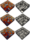Fig. 1. Left panels: normalised vertical velocity ${\stackrel{\sim }{u}}_z=u_z{(dg)}^{-1/2}$ (colour contours) and streamlines of the flow from runs C01 (PrSGS = 0.1, top panel), C1 (PrSGS = 1, middle), and C10 (PrSGS = 10, bottom). The colours of the streamlines indicate the local vertical velocity. Right panels: normalised entropy fluctuations $\stackrel{\sim }{s}\prime (\mathit{x})=[s(\mathit{x})-\overline{s}(z)]/s_{\mathrm{rms}}^{\prime }(z)$ from the same runs.

The averaged rms velocity as a function Pr_eff from all runs is shown in Fig. 2. There is a tendency for u_rms to increase with decreasing Pr_SGS which was first reported by Singh & Chan (1993) in compressible convection. Data for approximately constant Pe is suggestive of a power law with exponent around −0.13; see the dotted lines in Fig. 2. A similar dependence can be seen in the suitably scaled data of non-rotating spherical shell simulations R0P[1,2,6] of Karak et al. (2018); see the crosses in Fig. 2. However, their run with the highest Pr (R0P20) appears to be an outlier. The results of Orvedahl et al. (2018) also indicate an increase in kinetic energy as the Prandtl number decreases. Furthermore, qualitatively similar results have been reported from Boussinesq convection (e.g., Breuer et al. 2004; Scheel & Schumacher 2016), although in the work of these latter authors the dependence of u_rms on Pr is much steeper. This is because, in Rayleigh-Bénard convection, the total flux transported by convection depends strongly on the Prandtl number.

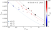Fig. 2. Volume- and time-averaged rms velocity as a function Preff(zCZ) for all of the current runs (circles). The colours (sizes) of the symbols indicate the Péclet number (relative error) as indicated in the colour bar (legend). The dotted lines show power laws proportional to ${\text{Pr}}_{\text{eff}}^{-0.13}$ for reference. The crosses show the scaled results from the non-rotating runs R0P[1,2,6,20] of Karak et al. (2018); see their Table 1.

A distinct characteristic of convection is that the vertical flows are the main transporter of the energy flux. A diagnostic of the structure of vertical flows is the filling factor f of up- or downflows. Here the filling factor is defined as the area the downflows occupy at each depth such that the horizontally averaged vertical velocity is given by

$$\begin{array}{c}\hfill {\overline{u}}_z(z)=f(z){\overline{u}}_z^{\downarrow }(z)+[1-f(z)]{\overline{u}}_z^{\uparrow }(z),\end{array}$$(25)

where ${\overline{u}}_z$ is the mean vertical velocity whereas ${\overline{u}}_z^{\downarrow }$ and ${\overline{u}}_z^{\uparrow }$ are the mean velocities in the down- and upflows, respectively. Figure 3a shows f for runs B01, B1, and B10 with Pr_SGS = 0.1, 1, and 10. These results indicate that the filling factor decreases with decreasing SGS Prandtl number. However, the change is relatively minor such that f differs by roughly 20% in the bulk of the CZ between the extreme cases with Pr_SGS = 0.1 and 10. The filling factor plays an important role in analytic and semi-analytic two-stream models of convection (e.g., Rempel 2004; Brandenburg 2016). For example, in the updated mixing length model of Brandenburg (2016), a very small filling factor is needed in cases where the Schwarzschild unstable part of the CZ is particularly shallow. The current simulations suggest that the filling factor goes in that direction when Pr_SGS decreases, but it appears that the smallest values of the order of 10⁻⁴ in some of the models of Rempel (2004) and Brandenburg (2016) are ruled out.

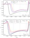Fig. 3. Filling factor of downflows for SGS Prandtl numbers 0.1 (solid line), 1 (dashed), and 10 (dash-dotted) as indicated by the legend from runs B01, B1, and B10 (a). Filling factor in runs with PrSGS = 0.1 with different PeSGS(b). The vertical dotted lines indicate the depths from which representative data for the top, middle, and bottom of the CZ are considered.

The filling factor increases as a function of Re and Pe_SGS for a given Pr_SGS; see Fig. 3b for representative results for Pr_SGS = 0.1 where χ_SGS ≫ χ. It is plausible that a growing contribution from nearly isotropic small-scale eddies that become more prominent with increasing Re is partly responsible for the increasing trend of f as a function of the Reynolds number. However, preliminary studies using low-pass filtered data suggest that this effect is very subtle. Irrespective of the Re dependence of f, the energetics of the underlying larger scale granulation appear to be almost unaffected by Re; see Sect. 3.3.

3.2. Overshooting below the convection zone

It is of interest to study the extent of convective overshooting below the CZ given the systematic dependence of the overall convective velocities on Pr_SGS. The same definition of overshooting as in Käpylä (2019a) is used. This is outlined by defining the bottom of the CZ (z_CZ) to be the depth where F̅_conv changes from positive to negative. This depth is used to obtain a reference value of the horizontally averaged kinetic energy flux ${{\overline{F}}_{\text{kin}}}^{\mathrm{ref}}={\overline{F}}_{\text{kin}}(z_{\text{CZ}},t)$. The instantaneous overshooting depth z_OS is then taken to be the depth where ${\overline{F}}_{\text{kin}}(z,t)$ drops below ${10}^{-2}{{\overline{F}}_{\text{kin}}}^{\mathrm{ref}}$. The mean thickness of the overshoot layer is defined as

$$\begin{array}{c}\hfill d_{\mathrm{os}}=\frac{1}{\mathrm{\Delta }t}{\displaystyle {\int }_{t_0}^{t_1}[z_{\mathrm{CZ}}(t)-z_{\mathrm{OS}}(t)]\mathrm{d}t,}\end{array}$$(26)

where Δt = t₁ − t₀, and t₀ and t₁ denote the beginning and end of the time-averaging period.

Figure 4 shows d_os from all runs as a function of Pr_SGS. The current results confirm the conjecture of Käpylä (2019a) that d_os is sensitive to the Prandtl number. However, the results still depend of the Péclet number especially for low Pr_SGS where it is challenging to reach high values of Pe. Nevertheless, comparing d_os for approximately the same Pe, for example Pe ≈ 40 (light blue symbols in Fig. 4), shows that the overshooting is increasing monotonically as Pr_SGS decreases. The difference in d_os between the cases Pr_SGS = 1 and Pr_SGS = 0.1 is about 30%. However, the difference decreases as the Péclet number increases; nevertheless it does not appear likely that the Pr dependence would disappear at even higher Péclet numbers.

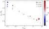Fig. 4. Thickness of the overshoot layer dos normalised by the pressure scale height Hp(zCZ) for all runs as a function of Preff(zCZ). The colours (sizes) of the symbols indicate the Péclet number (relative error) as indicated in the colour bar (legend).

Several numerical studies have shown that the deep parts of density-stratified CZs are often weakly stably stratified (e.g., Chan & Gigas 1992; Tremblay et al. 2015; Bekki et al. 2017; Hotta 2017; Käpylä et al. 2017). Such layers have also been found from semi-global and global simulations of rotating solar-like CZs (e.g., Karak et al. 2018; Käpylä et al. 2019; Viviani & Käpylä 2021) as well as from fully convective spheres (Käpylä 2021). We call this layer the Deardorff zone after Brandenburg (2016). This layer is characterised by a positive vertical gradient of entropy, ds/dz > 0, along with a positive convective energy flux, ${\overline{F}}_{\text{conv}}>0$. The mean thickness of the Deardorff zone is defined in a similar way to d_os via

$$\begin{array}{c}\hfill d_{\mathrm{DZ}}=\frac{1}{\mathrm{\Delta }t}{\displaystyle {\int }_{t_0}^{t_1}[z_{\mathrm{BZ}}(t)-z_{\mathrm{CZ}}(t)]\mathrm{d}t,}\end{array}$$(27)

where z_BZ is the depth where the entropy gradient changes sign. The results for d_DZ are shown in Fig. 5. At first glance, d_DZ shows an opposite trend in comparison to d_os such that it decreases with the Prandtl number but the dependence on Péclet and Reynolds numbers is again strong, particularly for low Pr_SGS. However, considering only the largest Pe for each Pr_eff, d_DZ is roughly constant around 0.45H_p for Pr_eff ≲ 3.

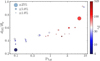Fig. 5. Thickness of the Deardorff layer dDZ normalised by the pressure scale height Hp(zCZ) for all runs as a function of Preff(zCZ). The colours (sizes) of the symbols indicate the Péclet number (relative error) as indicated in the colour bar (legend).

3.3. Flow statistics and spectral distribution

A standard diagnostics in flow statistics is the probability density function (PDF) which is defined by:

$$\begin{array}{c}\hfill {\displaystyle \int }\mathcal{P}(u_i,z)\mathrm{d}{u}_i=1.\end{array}$$(28)

The moments of the PDF carry information about the statistical properties of the flow. The instantaneous z-dependent moments are given by:

$$\begin{array}{c}\hfill {\mathcal{M}}^n(u_i,z)={\displaystyle \int }{[u_i(\mathit{x})-{\overline{u}}_i(z)]}^n\mathcal{P}(u_i,z)\mathrm{d}{u}_i.\end{array}$$(29)

Here we study the skewness 𝒮 and the kurtosis 𝒦 of the velocity field:

$$\begin{array}{c}\hfill \mathcal{S}=\frac{{\mathcal{M}}^3}{{\sigma }_u^3},\mathcal{K}=\frac{{\mathcal{M}}^4}{{\sigma }_u^4},\text{where}{\sigma }_u={({\mathcal{M}}^2)}^{1/2}.\end{array}$$(30)

Representative PDFs of the velocity components near the surface, at the middle, and near the base of the CZ from run C01 are shown in Fig. 6. The data are obtained by time-averaging over several snapshots. The horizontal flows have zero means and they have symmetric distributions around the mean. The vertical flows on the other hand show a bimodal distribution corresponding to the characteristic up- and downflow structure of convective granulation which is particularly clear near the surface. Similar results have been reported from a number of earlier numerical studies in different contexts and setups (e.g., Brandenburg et al. 1996; Miesch et al. 2008; Hotta et al. 2015).

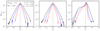Fig. 6. Normalised PDFs of ux (left panel), uy (middle), and uz (right) from near the surface (black lines), middle (blue), and bottom (red) of the CZ as indicated by the key for run C01 with Re = 190 and PrSGS = 0.1.

Figure 7 shows 𝒮 and 𝒦 as functions of depth from runs C01, C1, and C10. The skewness of the horizontal flows is essentially zero in all of the cases which is expected because no systematic horizontal anisotropy is present. 𝒮 is consistently negative and decreasing with depth for vertical flows within the CZ. This is indicative of a growing difference between the statistics of up- and downflows in the deeper parts. The kurtosis indicates a nearly Gaussian distribution with 𝒦 ≈ 3 for both vertical and horizontal flows near the surface (z/d ≈ 0.9). However, 𝒦 increases as a function of depth such that 𝒦 ≈ 5 for u_x and u_y, and has a value of greater than 10 for u_z at the base of the CZ, indicating strong non-Gaussianity. The skewness and kurtosis do not change significantly in the CZ as a function of Pr_SGS. The results for 𝒮 and 𝒦 are in agreement with those of Hotta et al. (2015) and similar to the rotating spherical shell simulations of Miesch et al. (2008) notwithstanding the horizontal anisotropy in the latter. Finally, 𝒦 reaches very high values in the overshoot regions especially for low Pr_SGS; see left panel of Fig. 7. This is most likely due to the highly intermittent turbulence which in turn is due to the limited number of deeply penetrating plumes in these regions.

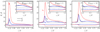Fig. 7. Kurtosis 𝒦 (solid lines) and skewness 𝒮 (dashed) of the velocity components from runs C01 (PrSGS = 0.1, left panel), C1 (PrSGS = 1, middle), and C10 (PrSGS = 10, right).

Next we study the velocity amplitudes as functions of spatial scale from power spectra of the velocity field,

$$\begin{array}{cc}\hfill E_{\mathrm{K}}(k,z,t)& =\frac{1}{2}{\displaystyle \sum _k{|\widehat{\mathit{u}}(k,z,t)|}^2,}\hfill \end{array}$$(31)

where $k=\sqrt{k_x^2+k_{\mathit{y}}^2}$ is the horizontal wavenumber and the hat denotes a two-dimensional Fourier transform. The power spectra are computed from between 10 and 40 snapshots –depending on the run– which are then time-averaged. Furthermore, normalisation is applied such that

$$\begin{array}{cc}\hfill {\stackrel{\sim }{E}}_{\mathrm{K}}(k,z)& =\frac{1}{\mathrm{\Delta }T}{\displaystyle {\int }_{T_0}^{T_1}\frac{E_{\mathrm{K}}(k,z,t)}{{\sum }_0^{k_{\mathrm{grid}}}{E}_{\mathrm{K}}(k,z,t)}\mathrm{d}t,}\hfill \end{array}$$(32)

where k_grid = nx_h/2 is the Nyquist scale of the horizontal grid with nx_h grid points. With this normalisation the differences in the shape of the spectra are highlighted whereas the differences in the absolute magnitude are hidden. This is justified here because we are currently interested in the effects of the Prandtl number on the distribution of power as a function of spatial scale.

Representative results for Pr_SGS = 0.1, 1, and 10 are shown in Fig. 8 from runs C01, C1, and C10. The differences in E_K are small and most clearly visible at high wavenumbers near the surface and near the base of the CZ. The power at the largest scales (k/k_H < 3) is similar in all cases and the clearest differences are seen at the base of the CZ although even these features are not particularly pronounced. It is possible that the horizontal extent of the domain is too small to capture the largest naturally excited scales because the peak of the power spectrum is always near the box scale. The spectra show a scaling that is consistently steeper than the Kolmogorov-Obukhov k^−5/3 spectrum. The Bolgiano-Obukhov scaling (Bolgiano 1959; Obukhov 1959) with k^−11/5 is more compatible with the data especially at large Re. However, the inertial range even in the current highest resolution simulations is very limited and the conclusions regarding scaling properties are quite uncertain. Furthermore, there is a puzzling spread of scaling exponents from convection simulations: early studies with modest inertial ranges suggested a k^−5/3 scaling (e.g., Cattaneo et al. 1991; Brandenburg et al. 1996; Porter & Woodward 2000) whereas more recent studies (e.g., Hotta et al. 2015; Featherstone & Hindman 2016) suggest clearly shallower scalings. On the other hand, power spectra of solar surface convection suggest significantly steeper (Yelles Chaouche et al. 2020, and references therein) scaling.

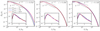Fig. 8. Normalised power spectra of velocity from depths z = 0.85d (left panel), z = 0.49d (middle), and z = 0.13d (right) for PrSGS = 0.1 (black lines), 1 (blue), and 10 (red) and Re = 167…190 corresponding to runs C01, C1, and C10, respectively. The insets show the low-wavenumber part of the spectra. The dashed and dotted lines respectively indicate the Bolgiano-Obukhov k−11/5 and Kolmogorov-Obukhov k−5/3 scalings for reference.

To study the anisotropy of the flow, the power spectra of vertical and horizontal velocities are defined as

$$\begin{array}{cc}\hfill {\displaystyle {\int }_0^{k_{\max }}}{E}_{\mathrm{V}}(k,z)\mathrm{d}k& =\frac{1}{2}\overline{u_z^2}(z),\hfill \end{array}$$(33)

$$\begin{array}{cc}\hfill {\displaystyle {\int }_0^{k_{\max }}}{E}_{\mathrm{H}}(k,z)\mathrm{d}k& =\frac{1}{2}[\overline{u_x^2}(z)+\overline{u_y^2}(z)].\hfill \end{array}$$(34)

The same averaging and normalisation as above are applied here. Representative results from the same runs as in Fig. 8 are shown in Fig. 9. The horizontal and vertical velocity power spectra at all depths indicate a dominance of horizontal flows at large scales (k ≲ 3) whereas vertical flows are dominant for larger k. The scaling of E_H is consistently steeper than the Kolmogorov-Obukhov k^−5/3 dependence.

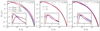Fig. 9. Normalised power spectra of vertical (EV, solid lines) and horizontal velocities (EH, dashed) from the same depths and runs as in Fig. 8. The inset shows low-wavenumber contributions.

However, the differences between runs are again small with the exception of the bottom of the CZ (z = 0.13d) where a reduction of E_H at large scales k/k_H ≤ 4 for Pr_SGS = 0.1 is seen. The changes in the spectra are relatively subtle and an alternative way to study the spectral distribution of velocity is to consider the spectral anisotropy parameter A_V which is defined as (Käpylä 2019b):

$$\begin{array}{c}\hfill A_{\mathrm{V}}(k,z)\equiv \frac{E_{\mathrm{H}}(k,z)-2E_{\mathrm{V}}(k,z)}{E_{\mathrm{K}}(k,z)}.\end{array}$$(35)

Results for A_V for the same runs as in Figs. 8 and 9 are shown in Fig. 10. Near the surface the large scales are dominated by horizontal flows such that A_V(k) > 0 for k < 4. The large-scale anisotropy for k/k_H < 10 is almost identical for the three simulations shown in Fig. 10. The run with the highest Pr_SGS starts to deviate from the other two for k/k_H > 10, and the two remaining runs deviate for k/k_H ≳ 150. Given that the energy transport is dominated by scales for which k/k_H ≲ 30 (see below), it is likely that the differences of A_V at large k/k_H are not of great importance. The anisotropy at the middle of the CZ is remarkably similar for all three cases such that significant deviations occur only for k/k_H ≳ 100; see the middle panel of Fig. 10. The situation changes dramatically at the base of the CZ: while A_V is essentially the same for all Prandtl numbers for k/k_H > 8, the results systematically deviate at larger scales. That is, the flow at largest scales (k/k_H = 1) continues to be horizontally dominated for all Prandtl numbers but A_V is decreasing monotonically with Pr_SGS such the for Pr_SGS = 0.1, A_V change of sign from positive to negative already for k/k_H > 1. This is reflecting the stronger downflows and deeper overshooting in the low-Pr_SGS regime.

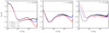Fig. 10. Spectral vertical anisotropy parameter AV(k) according to Eq. (35) from near the surface (z = 0.85d, left panel), middle (z = 0.49d, middle), and near the bottom of the CZ (z = 0.13d, right) for the same runs as in Fig. 8.

Figure 11 shows normalised velocity power spectra compensated by k^11/5 from five runs with Pr_SGS = 0.1 where the Reynolds number varies between 48 and 473. This figure shows that the scaling of the velocity spectra for the highest Reynolds numbers at low Pr_SGS is close to or even steeper than the Bolgiano-Obukhov k^−11/5 scaling. This is particularly clear at the middle and at the base of the CZ while no clear scaling can be discerned near the surface. Evidence for the Bolgiano-Obukhov scaling for the kinetic energy spectrum has previously been reported from simulations Rayleigh-Bénard convection (e.g., Calzavarini et al. 2002) as well as from corresponding shell models (Brandenburg 1992). However, the generality of the results for the spectra remain in question as stated earlier.

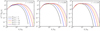Fig. 11. Power spectra of the velocity compensated by k11/5 from near the surface (z = 0.85d, left panel), middle (z = 0.49d, middle), and near the bottom of the CZ (z = 0.13d, right) for PrSGS = 0.1 as a function of the SGS Péclet number as indicated by the legend. The spectra are normalised such that the contributions from k/kH = 1 coincide.

The Bolgiano-Obukhov scaling is expected if the Bolgiano length is smaller than the typical turbulent length scale. In analogy with Rayleigh-Bénard convection (e.g., Calzavarini et al. 2002; Ching 2014), we define the Bolgiano length by

$$\begin{array}{c}\hfill {\ell }_{\mathrm{B}}=\frac{{ϵ}_u^{5/4}}{a_s{ϵ}_s^{3/4}+a_T{ϵ}_T^{3/4}},\end{array}$$(36)

where ${ϵ}_u=2\nu \overline{{\mathsf{S}}^2}$, ${ϵ}_s={\chi }_{\text{SGS}}\overline{{|\mathbf{\nabla }{s}^{\prime }|}^2}$, and ${ϵ}_T=\overline{{\chi |\mathbf{\nabla }T|}^2}$ are the horizontally averaged dissipation rates of kinetic energy and entropy fluctuations due to SGS and radiative diffusion, respectively. The factors a_s = (c_P/g²)^3/4 and a_T = (c_P/d)^3/2 enter due to dimensional arguments. The contribution from radiative diffusion ϵ_T is dominant in the denominator everywhere except near the surface where χ is very small. Representative results of ℓ_B are shown in Fig. 12 for runs C01, C1, and C10. We find that ℓ_B is of the order of 10⁻³…10⁻²d in the deep parts of the CZ and reaches maximum values of around 0.1d in the upper part of the CZ. Near the surface, l_B increases with Pr_SGS. The integral scale of turbulence is given by

$$\begin{array}{c}\hfill \ell =\frac{\int k^{-1}{E}_{\mathrm{K}}(k,z)\mathrm{d}k}{\int E_{\mathrm{K}}(k,z)\mathrm{d}k}.\end{array}$$(37)

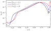Fig. 12. Normalised Bolgiano length ℓB/d according to Eq. (36) from runs C01 (black line), C1 (blue), and C10 (red).

We find that ℓ is generally in the range 0.35…0.45d irrespective of depth. This suggests that the Bolgiano-Obukhov scaling is indeed expected in the deep parts of the CZ. However, near the surface ℓ/ℓ_B ≈ 4 such that it is not obvious that the Bolgiano-Obukhov scaling should appear there. This is to some degree reflected by the simulation results where no clear power-law scaling can be seen near the surface (cf. left panel of Fig. 11).

The current results indicate that increasing Re, and therefore increasing Ra, does not significantly change the distribution of velocity power in wavenumber space. This is in apparent contradiction with the results of Featherstone & Hindman (2016) who reported an increase of small-scale flow amplitudes at the expense of large-scale power as the Rayleigh number was increased. However, in their study the increase of the Rayleigh number was associated with a significant change in the fraction of the energy flux that is carried by convection because their SGS entropy diffusion contributes to the mean energy flux; see their Fig. 6. It also appears that when the Rayleigh number is sufficiently large, the decrease in the large-scale power ceases also for Featherstone & Hindman (2016); see their Fig. 3. In the present study the convective flux is not directly influenced by the SGS entropy diffusion and thus the current results differ qualitatively from those of Featherstone & Hindman (2016).

Figure 13 shows compensated power spectra of specific entropy fluctuations from runs C01, C1, and C10. The spectra are compensated by k^11/6 which appears to be compatible with the highest Pe cases. For Pr_SGS = 0.1, there is no clear inertial range due to the low Péclet number in run C01. Runs C1 and C10, where the Péclet number is larger the entropy fluctuations, show roughly a k^−11/6 scaling at intermediate scales near the surface and at the middle of the CZ (top and middle panels of Fig. 13). Near the base of the CZ, only run C10 with the highest Pe shows signs of k^−11/6 spectra. The observed scaling is steeper than those from the Kolmogorov-Obukhov and Bolgiano-Obukhov models that predict k^−5/3 and k^−7/5, respectively. Based on the current results, it appears that the scaling of ${\stackrel{\sim }{E}}_S$ becomes progressively shallower as Pe increases such that neither of the theoretical predictions can be ruled out at the moment. However, simulations at even higher resolutions are needed to confirm this.

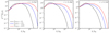Fig. 13. Power spectra of entropy fluctuations ${\stackrel{\sim }{E}}_S(k)$ compensated by k11/6 from near the surface (z = 0.85d, left panel), middle (z = 0.49d, middle), and near the bottom of the CZ (z = 13d, right) for runs C01 (black lines), C1 (blue), and C10 (red). The spectra are normalised such that the contributions from k/kH = 1 coincide.

3.4. Convective energy transport

Figure 14 shows the enthalpy, kinetic energy, and total convected fluxes –from Eqs. (20), (21), and (24), respectively– for the runs in set B with Re = 79…93 and 576³ grid. Remarkably, F̅_conv is almost identical within the CZ in all of the runs irrespective of the SGS Prandtl number. This indicates that the radiative flux and hence the thermal stratification and radiative conductivity are very similar in all of the runs. The constituents of the convective flux, however, show a very different behavior: the absolute values of the enthalpy and the kinetic energy fluxes increase monotonically with decreasing Pr_SGS. In particular, the kinetic energy flux more than doubles as Pr_SGS decreases from 10 to 0.1. For the lowest Pr_SGS, the downward kinetic energy flux exceeds F_bot near the middle of the CZ while F̅_enth is almost twice F_bot. In contrast to the CZ, the convected flux in the overshoot layer shows much larger differences between different Prandtl numbers.

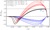Fig. 14. Normalised enthalpy (red), kinetic energy (blue), and convected (black) fluxes for the SGS Prandtl numbers ranging from 0.1 to 10 as indicated by the legend from the B set of runs with Re = 79…93.

The contributions of up- and downflows to the enthalpy, kinetic energy, and total convected flux F̅_conv are shown in Fig. 15. The contributions of the upflows to F̅_enth and ${\overline{F}}_{\text{kin}}$ increase monotonically as Pr_SGS decreases, leading to a net increase in the convected flux ${{\overline{F}}_{\text{conv}}}^{\uparrow }$. The magnitudes of ${\overline{F}}_{\text{enth}}^{\downarrow }$ and ${\overline{F}}_{\text{kin}}^{\downarrow }$ also increase as the SGS Prandtl number decreases but the net ${\overline{F}}_{\text{conv}}^{\downarrow }$ decreases because ${\overline{F}}_{\text{enth}}^{\downarrow }$ and ${\overline{F}}_{\text{kin}}^{\downarrow }$ have opposite signs. Remarkably, F̅_enth and ${\overline{F}}_{\text{kin}}$ are almost identical above z/d ≈ 0.9 irrespective of Pr_SGS, suggesting that near-surface physics are not the cause of the differences discussed here. In total, the up- and downflows transport on average an equal fraction of F̅_conv for SGS Prandtl number unity. The upflows are clearly dominant for the lowest SGS Prandtl numbers, such that for Pr_SGS = 0.1 the upflows transport roughly two-thirds of the convected flux within the CZ. An opposite, albeit weaker trend is seen for Pr_SGS > 1. The results for Pr_SGS ≠ 1 are thus qualitatively different from the case Pr_SGS = 1, and the difference increases towards larger and smaller Prandtl numbers. The current results are also in accordance with those of Cattaneo et al. (1991) who found that, in their more turbulent cases, the contribution of the downflows to F_conv diminishes. The increase in the level of turbulence in their cases was associated with a decreasing Prandtl number σ. In their simulations, the contribution of the downflows to the convected flux is practically negligible at σ = 0.1; see their Fig. 14d.

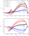Fig. 15. Contributions from upflows (a) and downflows (b) on the horizontally averaged convected (black lines), enthalpy (red), and kinetic energy (blue) fluxes for the same runs as in Fig. 14.

An important caveat of the current results is that changing Pr_SGS implies also that the Péclet number is changing. Therefore, it is necessary to test whether the observed differences are really due to the Prandtl number and not because of a Péclet number dependence. Such a check is shown in Fig. 16 where the convected flux from the five simulations with Pr_SGS = 0.1 (A01, B01, C01, C01b, and C01c) is compared. The Reynolds and Péclet numbers differ by an order of magnitude in this set of runs. The differences are minor within the CZ, whereas somewhat larger deviations are seen in the depth of the overshoot region. Nevertheless, the results are robust enough within the parameter range explored here such that the conclusions drawn regarding the energy fluxes remain valid. However, the current results should still be considered with some caution as the Péclet numbers studied thus far are still modest compared to realistic stellar conditions.

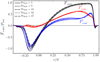Fig. 16. Comparison of total convected flux (black) and the contributions of the upflows (red) and downflows (blue) between runs A01, B01, C01, C01b, and C01c with PrSGS = 0.1.

Although the statistics of velocity and entropy fluctuations do not show drastic changes as a function of Pr_SGS, the convective energy transport is indeed strongly affected. In the following, the same procedure as in Nelson et al. (2018) is used to study the dominant scales in the different contributions to the convective flux. First, a low-pass filter is applied to the quantities that enter the expressions of the fluxes such that wavenumbers k < k_max are retained. For the enthalpy (kinetic energy) flux, this applies to the fluctuating vertical momentum flux (ρu_z)′ and temperature fluctuation T′ (kinetic energy $E_{\text{kin}}=\frac{1}{2}\rho {\mathit{u}}^2$ and vertical velocity u_z). The normalised, horizontally averaged enthalpy and kinetic energy fluxes up to k_max are then computed according to

$$\begin{array}{cc}\hfill {\stackrel{\sim }{\overline{F}}}_{\mathrm{enth}}(k_{\max },z)& =\frac{1}{\mathrm{\Delta }t}{\displaystyle {\int }_{t_0}^{t_1}\left[\frac{\overline{(\rho u_z{)}^{\prime }(z,k_{\max },t)T^{\prime }(z,k_{\max },t)}}{{\overline{F}}_{\mathrm{enth}}(z,t)}\right]\mathrm{d}t,}\hfill \end{array}$$(38)

$$\begin{array}{cc}\hfill {\stackrel{\sim }{\overline{F}}}_{\mathrm{kin}}(k_{\max },z)& =\frac{1}{\mathrm{\Delta }t}{\displaystyle {\int }_{t_0}^{t_1}\left[\frac{\overline{E_{\mathrm{kin}}(z,k_{\max },t)u_z(z,k_{\max },t)}}{{\overline{F}}_{\mathrm{kin}}(z,t)}\right]\mathrm{d}t.}\hfill \end{array}$$(39)

Representative results for Pr_SGS = 0.1, 1, and 10 are shown in Fig. 17 near the surface of the CZ. The current results indicate that for Pr_SGS = 0.1 the dominant contribution of the enthalpy flux comes from larger scales than for the kinetic energy flux. For Pr_SGS = 1 the situation is qualitatively unchanged but the difference in the dominant scales is much smaller. On the other hand, for Pr_SGS = 10 the behaviour is reversed although only at relatively large wavenumbers (k/k_H ≳ 20). These results suggest that while the dominant velocity scale is quite insensitive to changes of the Prandtl number, a stronger dependence exists in the convective energy transport.

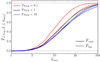Fig. 17. Spectrally decomposed, normalised enthalpy (${\stackrel{\sim }{\overline{F}}}_{\mathrm{enth}}$, solid lines) and kinetic energy (${\stackrel{\sim }{\overline{F}}}_{\mathrm{kin}}$, dashed lines) fluxes from z/d = 0.84 for runs C01 (red lines), C1 (black), and C10 (blue).

The current results thus suggest that convection becomes less efficient when the Prandtl number is decreased such that larger vertical velocities are required to carry the same flux. There are parallels between this and the Rayleigh-Bénard convection, where the Nusselt number decreases strongly for a given Rayleigh number when Pr is decreased (Schumacher & Sreenivasan 2020, and references therein). This means that low Prandtl number convection is very turbulent but at the same time inefficient in transporting heat. The analogy to the Reyleigh-Bénard case is, however, not complete as in the current simulations the ratio of convective to radiative flux is almost unchanged when the SGS Prandtl number changes. Therefore, the effects of the Prandtl number are necessarily much more subtle in the present cases and there is no straightforward way to connect, for example, the average rms-velocity and the Rayleigh number.

3.5. Velocity, temperature, and density fluctuations

The fact that the magnitudes of enthalpy and kinetic energy fluxes both increase as the SGS Prandtl number decreases while the total convected energy flux remains constant suggests a systematic change in the velocity and temperature fluctuations or their correlation as a function of Pr_SGS (for the latter, see Brandenburg et al. 2005). The rms-fluctuations of u_z for the total velocity, upflows, and downflows are shown in Fig. 18a for runs C01, C1, and C10. The rms vertical velocity in the bulk of the CZ increases monotonically for both up- and downflows as Pr_SGS decreases. The increase is particularly pronounced for the downflows, $u_z^{\text{rms}\downarrow }$, which is also the main contributor to the increase in $u_z^{\text{rms}}$. This reflects the decreasing filling factor of downflows with Pr_SGS (see Fig. 3a) such that the downflows need to be faster due to mass conservation.

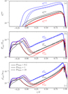Fig. 18. Horizontally averaged total rms vertical velocity (black lines) and the contributions from upflows (red) and downflows (blue) (a). Corresponding rms temperature (b) and density (c) fluctuations normalised by Ttop and ρtop = ρ0, respectively. Data for runs C01, C1, and C10 with PrSGS = 0.1, 1, and 10 are shown as indicated by the legend.

The temperature fluctuations shown in Fig. 18b show a somewhat more complex behaviour: near the surface $T_{\text{rms}}^{\prime }$ increases with Pr_SGS whereas in deeper parts the trend is reversed. This can be understood such that near the surface the temperature fluctuations are mostly in small-scale structures such as granules and intergranular lanes which are subject to stronger diffusion for smaller Pr_SGS, resulting in smaller $T_{\text{rms}}^{\prime }$ on average there. In the bulk of the CZ, $T_{\text{rms}}^{\prime }$ is the largest for the smallest Pr_SGS for both up- and downflows. This can partly explain the dominance of upflows in the energy transport for Pr_SGS = 0.1. For Pr_SGS = 1 and 10, $T_{\text{rms}}^{\prime }$ is always larger in the latter, which is due to the lower thermal diffusivity. Finally, Fig. 18c shows the depth dependence of the rms density fluctuations. Here a monotonic trend is seen such that ${\rho }_{\text{rms}}^{\prime }$ decreases with Pr_SGS.

The correlation coefficient of vertical velocity and temperature fluctuations is given by

$$\begin{array}{c}\hfill C[u_z,T\prime ]=\frac{\overline{u_{z}T\prime }}{u_z^{\mathrm{rms}}{T}_{\mathrm{rms}}^{\prime }}\approx \frac{{\overline{F}}_{\mathrm{enth}}}{c_{\mathrm{P}}\overline{\rho }{u}_z^{\mathrm{rms}}{T}_{\mathrm{rms}}^{\prime }},\end{array}$$(40)

where ${\overline{F}}_{\text{enth}}=c_{\text{P}}\overline{(\rho u_z)\prime T\prime }\approx c_{\text{P}}\overline{\rho }\overline{u_z^{\prime }{T}^{\prime }}$. The correlation coefficients C[u_z, T′] for the total flow, and up- and dowflows for the same runs as in Fig. 18 are shown in Fig. 19. The overall correlation coefficient C[u_z, T′] decreases monotonically as Pr_SGS increases, in agreement with Singh & Chan (1993). This trend is dominated by the downflows where $C[u_z^{\downarrow },T^{\prime \downarrow }]$ increases with decreasing Pr_SGS while a much weaker and opposite trend is observed for the upflows. The increasing correlation $C[u_z^{\downarrow },T^{\prime \downarrow }]$ with decreasing Pr_SGS explains the simultaneous strong increase in the magnitude of ${\overline{F}}_{\text{enth}}^{\downarrow }$. At the same time, the correlation in the upflows is much less affected by the SGS Prandtl number and the overall increase in vertical velocity and temperature fluctuations for low Pr_SGS (see, Fig. 18) explains the increased ${{\overline{F}}_{\text{enth}}}^{\uparrow }$ in that regime.

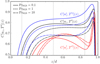Fig. 19. Correlation coefficient C[uz, T′] as a function of depth from run C01 (PrSGS = 0.1, solid lines), C1 (PrSGS = 1, dashed) and C10 (PrSGS = 10, dash-dotted) for the downflows (blue), upflows (red), and totals (black).

3.6. Driving of convection

The dependence of the convective flows on the Prandtl number raises the question of what is driving them. A primary candidate is the entropy gradient at the surface which has indeed reported to be Prandtl number dependent (e.g. Brandenburg et al. 2005). A diagnostic of this is the maximum value of the superadiabatic temperature gradient

$$\begin{array}{c}\hfill \mathrm{\Delta }\mathrm{\nabla }=\mathrm{\nabla }-{\mathrm{\nabla }}_{\mathrm{ad}}=-\frac{H_{\mathrm{p}}}{c_{\mathrm{P}}}\frac{\mathrm{d}s}{\mathrm{d}z},\end{array}$$(41)

where ∇ = ∂lnT/∂lnp and ∇_ad = 1 − 1/γ are the logarithmic and adiabatic temperature gradients, respectively. Figure 20 shows the maximum value of Δ∇ near the surface for the total entropy as well as for the upflow and downflow regions separately for all of the current runs. The results for max(Δ∇) show a decreasing trend as a function of Pe_eff and only a much weaker dependence on Pr_eff. The data perhaps suggest a (lnPe_eff)⁻¹ dependence. A similar decreasing trend is seen in the upflow regions although the scatter in the data is stronger especially in the intermediate range of Pe_eff. On the other hand, the data for the downflows perhaps suggest a plateau for Pe_eff ≳ 30. However, these tentative dependences are rather uncertain due to the limited data available. Nevertheless, it appears that for approximately the same Péclet number, the entropy gradient increases with Prandtl number. This is opposite to the trend in the strength of downflows and thus the surface entropy gradient cannot be the dominant contribution in driving the downflows.

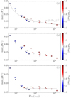Fig. 20. Maximum of the superadiabatic temperature gradient Δ∇=∇−∇ad as a function of the effective Péclet number at zsurf = 0.85d for the total (a), in upflows (b), and in downflows (c). The colour coding indicates Preff(zsurf).

Next we turn to the force balance for vertical flows. The horizontally averaged force density is given by

$$\begin{array}{c}\hfill {\overline{f}}_z=\overline{\rho \mathcal{D}{u}_z/\mathcal{D}t},\end{array}$$(42)

where 𝒟/𝒟t = ∂/∂t − u_z ∂_z is the vertical advective time derivative. Representative results for the total force are shown in Fig. 21a for runs C01, C1, and C10. The runs with SGS Prandtl numbers 1 and 10 show a small difference near the surface in that the maximum total force is slightly larger for the lower Prandtl number. On the other hand, ${\overline{f}}_z$ for Pr_SGS = 0.1 shows a markedly wider negative region in the upper part of the CZ between 0.65 ≲ z/d ≲ 0.9. The force on the upflows is shown in Fig. 21b. The differences between the two higher SGS Prandtl numbers are very small whereas the Pr_SGS = 0.1 case again shows a clear difference in the near-surface layers such that the region where upflows are decelerated is significantly wider. Remarkably, ${\overline{f}}_z^{\uparrow }$ is in almost perfect anticorrelation with the superadiabatic temperature gradient in the upflows (Δ∇^↑) such that upflows are decelerated (accelerated) in unstably (stably) stratified regions. This suggests that the upflows are not directly driven by the convective instability itself but rather by pressure forces induced by the deeply penetrating downflows (see also Korre et al. 2017; Käpylä et al. 2017). Finally, Fig. 21c shows the forces for the downflows. The downward force on the downflows is larger near the surface for Pr_SGS = 0.1 than in the cases with Pr_SGS = 1 and 10, which explains the stronger vertical velocities for low SGS Prandtl numbers. The force on the downflows is almost in anticorrelation with the overall superadiabatic temperature gradient; compare the grey and black lines in Fig. 21c³. The correlation with Δ∇^↓ is clearly poorer.

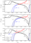Fig. 21. Horizontally averaged forces for the total flow (a), upflows (b) and downflows (c) for runs C01 (PrSGS = 0.1, solid lines), C1 (PrSGS = 1, dashed), and C10 (PrSGS = 10 dash-dotted). The blue and red lines show the corresponding superadiabatic temperature gradients with blue denoting negative and red positive values. The grey lines in panels b and c indicate Δ∇ for reference.

Figure 18c showed that the density fluctuations are weakly decreasing with Pr_SGS such that the increased acceleration on the downflows cannot be explained by arguing that the matter in the downflows is cooler and heavier in the low-Pr_SGS cases in comparison to the higher Pr_SGS cases. On the other hand, Fig. 19 shows that the correlation between vertical velocity and temperature fluctuations increases with decreasing Pr_SGS which is the decisive factor in the enhanced acceleration of downflows. A similar enhancement of correlation is likely to carry over to other thermodynamic quantities as well. The exact mechanism is unclear, but it seems plausible to assume that a process similar to the positive feedback loop between vertical flows and the buoyancy force in the zero Prandtl number limit in Rayleigh-Bénard convection (Spiegel 1962) is also present in the compressible case.

4. Conclusions

Convective energy transport and flow statistics are sensitive to the SGS Prandtl number in the parameter range currently accessible to numerical simulations. The most striking effect is the decrease in net energy transport due to downflows with decreasing Prandtl number. This happens because the oppositely signed enthalpy and kinetic energy fluxes both increase in the downflows, leading to increased cancellation (Cattaneo et al. 1991). Another effect of a decreasing Prandtl number is the increase in the overall velocity which is mostly due to the increase in the downflow strength. The stronger downflows also lead to much stronger overshooting at the base of the CZ for lower Prandtl numbers.

On the other hand, the effects of the Prandtl number are very subtle in the statistics of the velocity field. The clearest systematic effect is that the filling factor of downflows decreases monotonically with decreasing SGS Prandtl number. However, the power spectra of velocity show very small differences, apart from the deep layers where the downflow dominance in the low-Prandtl number regime becomes more prominent. The current results do not indicate a decrease in the large-scale velocity power either with decreasing Prandtl or with increasing Rayleigh numbers. Such a decrease has been suggested to be at least a partial solution to the convective conundrum, or the overly high large-scale power in simulated flows (Featherstone & Hindman 2016). In the current simulations, the large-scale power is almost unaffected, most likely because the SGS entropy diffusion does not contribute to the mean energy flux unlike in the simulations of Featherstone & Hindman (2016). Notably, however, the dominant spatial scales of enthalpy and kinetic energy fluxes vary systematically with Pr_SGS which is likely to hold the key to understanding the changing convective dynamics.

The implications of the current results of solar and stellar convection are difficult to assess because of the greatly differing parameter regimes of the simulations compared to stellar CZs. Another aspect is that the current simulations are very likely not in an asymptotic regime such that the results show a dependence on the Reynolds and Péclet numbers. Nevertheless, even with these reservations, it appears likely that convection in the Sun is quite different from that obtained from simulations in which Pr ≈ 1. In particular, the overshooting depth can be substantially underestimated by the current simulations. It is also unclear as to how the Prandtl number effects manifest themselves in angular momentum transport which has thus far only been discussed in the Pr ≳ 1 regime (Karak et al. 2018).

The current simulations use SGS diffusion for the entropy fluctuations which is solely because of numerical convenience. The use of SGS diffusion has been criticised because it is typically not rigorously formulated and because it is possibly affecting the resolved convective energy flux indirectly. We will address these questions in a separate paper with simulations where the SGS diffusion is absent.

Acknowledgments

I thank the anonymous referee, Axel Brandenburg, and Nishant Singh for their comments on the manuscript. I acknowledge the hospitality of Nordita during the program “The Shifting Paradigm of Stellar Convection: From Mixing Length Concepts to Realistic Turbulence Modelling.” The simulations were made within the Gauss Centre for Supercomputing project “Cracking the Convective Conundrum” in the Leibniz Supercomputing Centre’s SuperMUC–NG supercomputer in Garching, Germany. This work was supported by the Deutsche Forschungsgemeinschaft Heisenberg programme (grant No. KA 4825/2-1).

References

All Tables

All Figures

Fig. 1. Left panels: normalised vertical velocity ${\stackrel{\sim }{u}}_z=u_z{(dg)}^{-1/2}$ (colour contours) and streamlines of the flow from runs C01 (PrSGS = 0.1, top panel), C1 (PrSGS = 1, middle), and C10 (PrSGS = 10, bottom). The colours of the streamlines indicate the local vertical velocity. Right panels: normalised entropy fluctuations $\stackrel{\sim }{s}\prime (\mathit{x})=[s(\mathit{x})-\overline{s}(z)]/s_{\mathrm{rms}}^{\prime }(z)$ from the same runs.

In the text

Fig. 2. Volume- and time-averaged rms velocity as a function Preff(zCZ) for all of the current runs (circles). The colours (sizes) of the symbols indicate the Péclet number (relative error) as indicated in the colour bar (legend). The dotted lines show power laws proportional to ${\text{Pr}}_{\text{eff}}^{-0.13}$ for reference. The crosses show the scaled results from the non-rotating runs R0P[1,2,6,20] of Karak et al. (2018); see their Table 1.

In the text

	Fig. 3. Filling factor of downflows for SGS Prandtl numbers 0.1 (solid line), 1 (dashed), and 10 (dash-dotted) as indicated by the legend from runs B01, B1, and B10 (a). Filling factor in runs with PrSGS = 0.1 with different PeSGS(b). The vertical dotted lines indicate the depths from which representative data for the top, middle, and bottom of the CZ are considered.
In the text

	Fig. 4. Thickness of the overshoot layer dos normalised by the pressure scale height Hp(zCZ) for all runs as a function of Preff(zCZ). The colours (sizes) of the symbols indicate the Péclet number (relative error) as indicated in the colour bar (legend).
In the text

	Fig. 5. Thickness of the Deardorff layer dDZ normalised by the pressure scale height Hp(zCZ) for all runs as a function of Preff(zCZ). The colours (sizes) of the symbols indicate the Péclet number (relative error) as indicated in the colour bar (legend).
In the text

	Fig. 6. Normalised PDFs of ux (left panel), uy (middle), and uz (right) from near the surface (black lines), middle (blue), and bottom (red) of the CZ as indicated by the key for run C01 with Re = 190 and PrSGS = 0.1.
In the text

	Fig. 7. Kurtosis 𝒦 (solid lines) and skewness 𝒮 (dashed) of the velocity components from runs C01 (PrSGS = 0.1, left panel), C1 (PrSGS = 1, middle), and C10 (PrSGS = 10, right).
In the text

Fig. 8. Normalised power spectra of velocity from depths z = 0.85d (left panel), z = 0.49d (middle), and z = 0.13d (right) for PrSGS = 0.1 (black lines), 1 (blue), and 10 (red) and Re = 167…190 corresponding to runs C01, C1, and C10, respectively. The insets show the low-wavenumber part of the spectra. The dashed and dotted lines respectively indicate the Bolgiano-Obukhov k−11/5 and Kolmogorov-Obukhov k−5/3 scalings for reference.

In the text

	Fig. 9. Normalised power spectra of vertical (EV, solid lines) and horizontal velocities (EH, dashed) from the same depths and runs as in Fig. 8. The inset shows low-wavenumber contributions.
In the text

	Fig. 10. Spectral vertical anisotropy parameter AV(k) according to Eq. (35) from near the surface (z = 0.85d, left panel), middle (z = 0.49d, middle), and near the bottom of the CZ (z = 0.13d, right) for the same runs as in Fig. 8.
In the text

	Fig. 11. Power spectra of the velocity compensated by k11/5 from near the surface (z = 0.85d, left panel), middle (z = 0.49d, middle), and near the bottom of the CZ (z = 0.13d, right) for PrSGS = 0.1 as a function of the SGS Péclet number as indicated by the legend. The spectra are normalised such that the contributions from k/kH = 1 coincide.
In the text

	Fig. 12. Normalised Bolgiano length ℓB/d according to Eq. (36) from runs C01 (black line), C1 (blue), and C10 (red).
In the text

	Fig. 13. Power spectra of entropy fluctuations ${\stackrel{\sim }{E}}_S(k)$ compensated by k11/6 from near the surface (z = 0.85d, left panel), middle (z = 0.49d, middle), and near the bottom of the CZ (z = 13d, right) for runs C01 (black lines), C1 (blue), and C10 (red). The spectra are normalised such that the contributions from k/kH = 1 coincide.
In the text

	Fig. 14. Normalised enthalpy (red), kinetic energy (blue), and convected (black) fluxes for the SGS Prandtl numbers ranging from 0.1 to 10 as indicated by the legend from the B set of runs with Re = 79…93.
In the text

	Fig. 15. Contributions from upflows (a) and downflows (b) on the horizontally averaged convected (black lines), enthalpy (red), and kinetic energy (blue) fluxes for the same runs as in Fig. 14.
In the text

	Fig. 16. Comparison of total convected flux (black) and the contributions of the upflows (red) and downflows (blue) between runs A01, B01, C01, C01b, and C01c with PrSGS = 0.1.
In the text

	Fig. 17. Spectrally decomposed, normalised enthalpy (${\stackrel{\sim }{\overline{F}}}_{\mathrm{enth}}$, solid lines) and kinetic energy (${\stackrel{\sim }{\overline{F}}}_{\mathrm{kin}}$, dashed lines) fluxes from z/d = 0.84 for runs C01 (red lines), C1 (black), and C10 (blue).
In the text

	Fig. 18. Horizontally averaged total rms vertical velocity (black lines) and the contributions from upflows (red) and downflows (blue) (a). Corresponding rms temperature (b) and density (c) fluctuations normalised by Ttop and ρtop = ρ0, respectively. Data for runs C01, C1, and C10 with PrSGS = 0.1, 1, and 10 are shown as indicated by the legend.
In the text

	Fig. 19. Correlation coefficient C[uz, T′] as a function of depth from run C01 (PrSGS = 0.1, solid lines), C1 (PrSGS = 1, dashed) and C10 (PrSGS = 10, dash-dotted) for the downflows (blue), upflows (red), and totals (black).
In the text

	Fig. 20. Maximum of the superadiabatic temperature gradient Δ∇=∇−∇ad as a function of the effective Péclet number at zsurf = 0.85d for the total (a), in upflows (b), and in downflows (c). The colour coding indicates Preff(zsurf).
In the text

	Fig. 21. Horizontally averaged forces for the total flow (a), upflows (b) and downflows (c) for runs C01 (PrSGS = 0.1, solid lines), C1 (PrSGS = 1, dashed), and C10 (PrSGS = 10 dash-dotted). The blue and red lines show the corresponding superadiabatic temperature gradients with blue denoting negative and red positive values. The grey lines in panels b and c indicate Δ∇ for reference.
In the text

References

- Augustson, K. C., Brun, A. S., & Toomre, J. 2019, ApJ, 876, 83 [Google Scholar]
- Barekat, A., & Brandenburg, A. 2014, A&A, 571, A68 [NASA ADS] [CrossRef] [EDP Sciences] [Google Scholar]
- Bekki, Y., Hotta, H., & Yokoyama, T. 2017, ApJ, 851, 74 [NASA ADS] [CrossRef] [Google Scholar]
- Bolgiano, R. 1959, J. Geophys. Res., 64, 2226 [NASA ADS] [CrossRef] [Google Scholar]
- Brandenburg, A. 1992, Phys. Rev. Lett., 69, 605 [CrossRef] [Google Scholar]
- Brandenburg, A. 2003, Computational Aspects of Astrophysical MHD and Turbulence, eds. A. Ferriz-Mas, & M. Núñez (London: Taylor and Francis), 269 [Google Scholar]
- Brandenburg, A. 2016, ApJ, 832, 6 [Google Scholar]
- Brandenburg, A., Jennings, R. L., Nordlund, Å., et al. 1996, J. Fluid Mech., 306, 325 [NASA ADS] [CrossRef] [Google Scholar]
- Brandenburg, A., Nordlund, A., & Stein, R. F. 2000, in Geophysical and Astrophysical Convection, Contributions from a workshop sponsored by the Geophysical Turbulence Program at the National Center for Atmospheric Research, October 1995, eds. P. A. Fox, & R. M. Kerr (The Netherlands: Gordon and Breach Science Publishers), 85 [Google Scholar]
- Brandenburg, A., Chan, K. L., Nordlund, Å., & Stein, R. F. 2005, Astron. Nachr., 326, 681 [NASA ADS] [CrossRef] [Google Scholar]
- Breuer, M., Wessling, S., Schmalzl, J., & Hansen, U. 2004, Phys. Rev. E, 69, 026302 [NASA ADS] [CrossRef] [Google Scholar]
- Calzavarini, E., Toschi, F., & Tripiccione, R. 2002, Phys. Rev. E, 66, 016304 [NASA ADS] [CrossRef] [Google Scholar]
- Cattaneo, F., Brummell, N. H., Toomre, J., Malagoli, A., & Hurlburt, N. E. 1991, ApJ, 370, 282 [CrossRef] [Google Scholar]
- Chan, K. L., & Gigas, D. 1992, ApJ, 389, L87 [NASA ADS] [CrossRef] [Google Scholar]
- Chan, K. L., & Sofia, S. 1986, ApJ, 307, 222 [NASA ADS] [CrossRef] [Google Scholar]
- Ching, E. S. C. 2014, Statistics and Scaling in Turbulent Rayleigh-Bénard Convection (Singapore: Springer Singapore) [CrossRef] [Google Scholar]
- Cossette, J.-F., & Rast, M. P. 2016, ApJ, 829, L17 [Google Scholar]
- Deardorff, J. W. 1961, J. Atmos. Sci., 18, 540 [NASA ADS] [Google Scholar]
- Deardorff, J. W. 1966, J. Atmos. Sci., 23, 503 [NASA ADS] [CrossRef] [Google Scholar]
- Dobler, W., Stix, M., & Brandenburg, A. 2006, ApJ, 638, 336 [NASA ADS] [CrossRef] [Google Scholar]
- Fan, Y., & Fang, F. 2014, ApJ, 789, 35 [NASA ADS] [CrossRef] [Google Scholar]
- Featherstone, N. A., & Hindman, B. W. 2016, ApJ, 818, 32 [NASA ADS] [CrossRef] [Google Scholar]
- Greer, B. J., Hindman, B. W., Featherstone, N. A., & Toomre, J. 2015, ApJ, 803, L17 [Google Scholar]
- Hanasoge, S. M., Duvall, T. L., & Sreenivasan, K. R. 2012, Proc. Natl. Acad. Sci., 109, 11928 [Google Scholar]
- Hanasoge, S., Gizon, L., & Sreenivasan, K. R. 2016, Ann. Rev. Fluid Mech., 48, 191 [Google Scholar]
- Hotta, H. 2017, ApJ, 843, 52 [Google Scholar]
- Hotta, H., Rempel, M., & Yokoyama, T. 2015, ApJ, 803, 42 [NASA ADS] [CrossRef] [Google Scholar]
- Hotta, H., Iijima, H., & Kusano, K. 2019, Sci. Adv., 5, 2307 [Google Scholar]
- Käpylä, P. J. 2011, Astron. Nachr., 332, 43 [CrossRef] [Google Scholar]
- Käpylä, P. J. 2019a, A&A, 631, A122 [NASA ADS] [CrossRef] [EDP Sciences] [Google Scholar]
- Käpylä, P. J. 2019b, Astron. Nachr., 340, 744 [CrossRef] [Google Scholar]
- Käpylä, P. J. 2021, A&A, 655, A66 [CrossRef] [Google Scholar]
- Käpylä, P. J., Käpylä, M. J., & Brandenburg, A. 2014, A&A, 570, A43 [NASA ADS] [CrossRef] [EDP Sciences] [Google Scholar]
- Käpylä, P. J., Rheinhardt, M., Brandenburg, A., et al. 2017, ApJ, 845, L23 [CrossRef] [Google Scholar]
- Käpylä, P. J., Viviani, M., Käpylä, M. J., Brandenburg, A., & Spada, F. 2019, Geophys. Astrophys. Fluid Dyn., 113, 149 [CrossRef] [Google Scholar]
- Karak, B. B., Miesch, M., & Bekki, Y. 2018, Phys. Fluids, 30, 046602 [NASA ADS] [CrossRef] [Google Scholar]
- Korre, L., Brummell, N., & Garaud, P. 2017, Phys. Rev. E, 96, 033104 [NASA ADS] [CrossRef] [Google Scholar]
- Kupka, F., & Muthsam, H. J. 2017, Liv. Rev. Comp. Astrophys., 3, 1 [NASA ADS] [CrossRef] [Google Scholar]
- Miesch, M. S., Brun, A. S., DeRosa, M. L., & Toomre, J. 2008, ApJ, 673, 557 [NASA ADS] [CrossRef] [Google Scholar]
- Nelson, N. J., Featherstone, N. A., Miesch, M. S., & Toomre, J. 2018, ApJ, 859, 117 [Google Scholar]
- Obukhov, A. M. 1959, Akademiia Nauk SSSR Doklady, 125, 1246 [Google Scholar]
- O’Mara, B., Miesch, M. S., Featherstone, N. A., & Augustson, K. C. 2016, Adv. Space Res., 58, 1475 [CrossRef] [Google Scholar]
- Orvedahl, R. J., Calkins, M. A., Featherstone, N. A., & Hindman, B. W. 2018, ApJ, 856, 13 [NASA ADS] [CrossRef] [Google Scholar]
- Ossendrijver, M. 2003, A&ARv., 11, 287 [NASA ADS] [CrossRef] [Google Scholar]
- Pencil Code Collaboration (Brandenburg, A., et al.) 2021, J. Open Source Softw., 6, 2807 [Google Scholar]
- Porter, D. H., & Woodward, P. R. 2000, ApJS, 127, 159 [NASA ADS] [CrossRef] [Google Scholar]
- Rempel, M. 2004, ApJ, 607, 1046 [Google Scholar]
- Roxburgh, L. W., & Simmons, J. 1993, A&A, 277, 93 [NASA ADS] [Google Scholar]
- Scheel, J. D., & Schumacher, J. 2016, J. Fluid Mech., 802, 147 [NASA ADS] [CrossRef] [Google Scholar]
- Schumacher, J., & Sreenivasan, K. R. 2020, Rev. Mod. Phys., 92, 041001 [NASA ADS] [CrossRef] [Google Scholar]
- Singh, H. P., & Chan, K. L. 1993, A&A, 279, 107 [Google Scholar]
- Spiegel, E. A. 1962, J. Geophys. Res., 67, 3063 [NASA ADS] [CrossRef] [Google Scholar]
- Spruit, H. 1997, Mem. Soc. Astron. It., 68, 397 [Google Scholar]
- Tremblay, P.-E., Ludwig, H.-G., Freytag, B., et al. 2015, ApJ, 799, 142 [Google Scholar]
- Viviani, M., & Käpylä, M. J. 2021, A&A, 645, A141 [EDP Sciences] [Google Scholar]
- Weiss, A., Hillebrandt, W., Thomas, H.-C., & Ritter, H. 2004, Cox and Giuli’s Principles of Stellar Structure (Cambridge, UK: Cambridge Scientific Publishers Ltd) [Google Scholar]
- Yelles Chaouche, L., Cameron, R. H., Solanki, S. K., et al. 2020, A&A, 644, A44 [NASA ADS] [CrossRef] [EDP Sciences] [Google Scholar]