© The Authors 2025

1. Introduction

It has become evident during the last decade and a half that the theoretical understanding of convection in the Sun is not as complete as previously thought (e.g. Hanasoge et al. 2010, 2012; Schumacher & Sreenivasan 2020). This is because helioseismology and other solar observations suggest that velocity amplitudes on large scales on the Sun are much lower than in current simulations (e.g. Birch et al. 2024, and references therein). This discrepancy is commonly referred to as the convective conundrum (O’Mara et al. 2016), and it is the most likely reason why global magnetohydrodynamic simulations of the Sun struggle to reproduce the solar differential rotation and large-scale dynamo (e.g. Käpylä et al. 2023, and references therein). This has led to a re-evaluation of the fundamental theory of stellar convection.

In the widely used mixing length theory (e.g. Vitense 1953; Joyce & Tayar 2023), convection is driven locally by an unstable temperature gradient in accordance with the Schwarzschild criterion. On the other hand, solar surface simulations (e.g. Stein & Nordlund 1998) suggest that convection in the Sun is driven by surface cooling due to a rain of low entropy material that forms strong downflow plumes. Such entropy rain is highly non-local and has been suggested to be relevant for deep convection as well (Spruit 1997), and to lead to a convection zone that is weakly stably stratified (Brandenburg 2016). Recent studies of global Rossby waves in the Sun indeed suggest that the solar convection zone has to be either very nearly adiabatic (Gizon et al. 2021) or mildly subadiabatic (Bekki 2024).

Simulations of compressible convection have confirmed the existence of subadiabatic layers in the deep parts of convective envelopes (e.g. Roxburgh & Simmons 1993; Tremblay et al. 2015; Bekki et al. 2017; Hotta 2017; Käpylä et al. 2017; Brun et al. 2022; Käpylä 2021, 2024a). However, in all of these simulations the subadiabatic layer at the base of the convection zone encompasses a relatively small fraction of the total depth of the convective layer. It is possible that this is the configuration in the Sun and in other stars with convective envelopes. Another possibility is that the current simulations do not capture the entropy rain originating near the surface accurately due to insufficient resolution. This is plausible because the parameter regime of the Sun is prohibitively far away from the range accessible to current simulations (e.g. Kupka & Muthsam 2017; Käpylä et al. 2023). The resolution issue is particularly dire in the photosphere where the gas becomes optically thin abruptly over a distance of several tens of kilometres and coincides with the layer where entropy rain is thought to be launched. A few earlier numerical studies have explored surface effects on deep convection zone structure. For example, Cossette & Rast (2016) and Yokoi et al. (2022) find that increased surface forcing, corresponding to a steeper entropy gradient, leads to reduced scale of convection in deep layers. A similar approach was used in Käpylä (2024b) where stronger surface forcing resulted in deeper convection zones due to a thermodynamics-dependent heat conductivity. On the other hand, Hotta & Kusano (2021) find that the properties of the surface layers have a negligible effect on deep convection in a simulation that covers the entire density contrast of the solar convection zone.

In the current study, the working hypothesis is that the surface effects occur on scales that cannot be resolved directly in current simulations. Here the surface-induced entropy rain is modelled by non-uniform cooling where localised cool patches lead to plume formation. This is motivated by the non-uniform surface temperature in the Sun. A similar approach was taken by Nelson et al. (2018), who studied convection in rotating spherical shells and included a prescribed impulse acting on the generated plumes with the aim of studying global phenomena such as differential rotation. At the other end of the spectrum are the studies of Rieutord & Zahn (1995), Rast (1998) and Anders et al. (2019), who investigated individual plumes in a non-convecting background. Here these studies are generalised to cases with a convective background while retaining simple geometry and omitting the effects of rotation and magnetism. The primary aim is to explore the transition to entropy-rain-dominated convection and its implications for thermal and flow structures in the convection zone.

2. The model

The model is based on that used in Käpylä (2019a, 2021, 2024a), and the PENCIL CODE (Pencil Code Collaboration 2021)¹ was used to produce the simulations. The equations for compressible hydrodynamics were solved:

$$\begin{array}{cc}\hfill \frac{Dln\rho }{\mathit{Dt}}& =-\mathbf{\nabla }\mathbf{·}\mathit{u},\hfill \end{array}$$(1)

$$\begin{array}{cc}\hfill \frac{D\mathit{u}}{\mathit{Dt}}& =\mathit{g}-\frac{1}{\rho }(\mathbf{\nabla }p-\mathbf{\nabla }\mathbf{·}2\nu \rho \mathsf{S}),\hfill \end{array}$$(2)

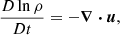
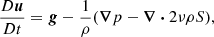
$$\begin{array}{cc}\hfill T\frac{\mathit{Ds}}{\mathit{Dt}}& =-\frac{1}{\rho }[\mathbf{\nabla }\mathbf{·}({\mathit{F}}_{\mathrm{rad}}+{\mathit{F}}_{\mathrm{SGS}})+\mathcal{C}]+2\nu {\mathsf{S}}^2,\hfill \end{array}$$(3)

where D/D_t = ∂/∂t + u · ∇ is the advective derivative, ρ is the density, u is the velocity, $\mathbf{g}=-g{\widehat{\mathbf{e}}}_z$ is the acceleration due to gravity, p is the pressure, T is the temperature, s is the specific entropy, and ν is the constant kinematic viscosity. The terms F_rad and F_SGS are the radiative and turbulent subgrid-scale (SGS) fluxes, respectively, and 𝒞 describes cooling near the surface. S is the traceless rate-of-strain tensor with 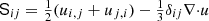${\mathsf{S}}_{\mathit{ij}}=\frac{1}{2}(u_{i,j}+u_{j,i})-\frac{1}{3}{\delta }_{\mathit{ij}}\mathrm{\nabla }·\mathbf{u}$. The gas is assumed to be optically thick and fully ionised where radiation is modelled via the diffusion approximation. The ideal gas equation of state, $p=(c_{\text{P}}-c_{\text{V}})\rho T=\mathcal{R}\rho T$, applies, where ℛ is the gas constant, and c_P and c_V are the specific heats at constant pressure and volume, respectively. The radiative flux is given by F_rad = −K∇T, where K is the radiative heat conductivity, given by K(ρ, T) = K₀(ρ/ρ₀)^{−(a + 1)}(T/T₀)^3 − b. The choice a = 1 and b = −7/2 corresponds to Kramers opacity law (Weiss et al. 2004), which was first used in convection simulations by Edwards (1990) and Brandenburg et al. (2000). Turbulent SGS flux, ${\mathbf{F}}_{\mathrm{SGS}}=-{\chi }_{\text{SGS}}\rho T\mathrm{\nabla }s\prime$, applies to the entropy fluctuations, $s\prime (\mathbf{x})=s(\mathbf{x})-\overline{s}(z)$, where the overbar indicates horizontal averaging and where χ_SGS is a constant. F_SGS has a negligible contribution to the net energy flux such that ${\overline{\mathbf{F}}}_{\mathrm{SGS}}\approx 0$. The cooling function 𝒞 consists of two parts: uniform cooling towards a constant temperature above z_cool, and additional n_patch local patches where the cooling is applied already at a lower depth z_patch < z_cool. The cooling function is described in Appendix A. The advective terms in Equations (1)–(3) contain a hyperdiffusive sixth-order correction with a flow-dependent diffusion coefficient (see Appendix B of Dobler et al. 2006).

The computational domain extends between z_bot​ ≤ z​ ≤ ​z_top, where z_bot/d​ = ​ − 0.45 or z_bot/d​ = ​ − 0.95 depending on the model, z_top/d​ = ​1.05, and the horizontal coordinates x and y run from −2d to 2d. The initial stratification consists of three layers. The two lower layers are polytropic with polytropic indices n₁​ = ​3.25 (z_bot/d​ ≤ ​z/d​ ≤ 0) and n₂​ = ​1.5 (0​ ≤ ​z/d​ ≤ 1). The latter corresponds to a marginally stable isentropic stratification. At t​ = ​0 the uppermost layer above z/d​ = ​1 is isothermal, and convection ensues because the system is not in thermal equilibrium. The velocity field is perturbed with small-scale Gaussian noise with an amplitude of ${10}^{-5}\sqrt{\mathit{dg}}$. Horizontal boundaries are periodic, and vertical boundaries are impenetrable and stress free. A constant energy flux is imposed at the lower boundary by setting ∂_zT = −F_bot/K_bot, where F_bot is a fixed input flux and K_bot​ = ​K(x, y, z_bot). A constant temperature T = T_top is imposed on the upper vertical boundary.

The units of length, time, density, and entropy are given by $[x]=d,[t]=\sqrt{d/g},[\rho ]={\rho }_0,[s]=c_{\text{P}}$, respectively, where ρ₀ is the initial value of density at z = z_top. The models are fully defined by choosing the values of ν, g, a, b, K₀, ρ₀, T₀, and the SGS Prandtl number Pr_SGS​ = ​ν/χ_SGS, along with the parameters of the cooling function. The quantity, ξ₀​ = ​H_p^top/d​ = ​ℛT_top/gd​ = ​0.054, is the initial pressure scale height at the surface. The Prandtl number based on the radiative heat conductivity is Pr(x) = ν/χ(x), where $\chi (\mathbf{x})=K(\mathbf{x})/c_{\text{P}}\rho (\mathbf{x})$. The dimensionless normalised flux is given by ℱ_n(z_bot)​ = ​F_bot/ρ(z_bot)c_s³(z_bot), where ρ(z_bot) and c_s(z_bot) are the density and the sound speed, respectively, at z/d​ = ​ − 0.45 at t = 0. The input flux is chosen to be much higher than the solar value (ℱ_n^⊙ ≈ 4 ⋅ 10⁻¹¹) to avoid a prohibitively long thermal saturation phase (e.g. Brandenburg et al. 2005; Käpylä et al. 2007). The Rayleigh number based on the energy flux is given by Ra_F = gd⁴F_bot/(c_PρTνχ²).

The Reynolds and SGS Péclet numbers are given by Re​ = ​u_rms/νk₁ and Pe_SGS​ = ​Pr_SGSRe​ = ​u_rms/χ_SGSk₁, where u_rms is the rms velocity averaged over the convectively mixed layer, and where k₁​ = ​2π/d. The total thermal diffusivity is given by ${\chi }_{\text{eff}}(\mathbf{x})={\chi }_{\text{SGS}}+\chi (\mathbf{x})$. The turbulent Rayleigh number, ${\text{Ra}}_{\text{t}}=\frac{g{d}^4}{\nu {\overline{\chi }}_{\text{eff}}}(-\frac{1}{c_{\text{P}}}\frac{\mathrm{d}\overline{s}}{\mathrm{d}z})$, is quoted from z/d = 0.85 in the statistically stationary state using the temporally and horizontally averaged mean state denoted by the overbars. The kinematic viscosity, ν, and SGS entropy diffusivity, χ_SGS, are chosen such that the flow remains resolved on the grid with average grid Reynolds and SGS Péclet numbers of the order of unity.

3. Results

To study the structure of the convection zone, the dominant contributions to the vertical energy flux need to be identified. These are given by

$$\begin{array}{cc}\hfill {\overline{F}}_{\mathrm{enth}}& =c_{\mathrm{P}}\overline{{(\rho u_z)}^{\prime }{T}^{\prime }},{\overline{F}}_{\mathrm{kin}}=\frac{1}{2}\overline{\rho {\mathit{u}}^2{u}_z^{\prime }},\hfill \end{array}$$(4)

$$\begin{array}{cc}\hfill {\overline{F}}_{\mathrm{rad}}& =-\overline{K}{\partial }_z\overline{T},{\overline{F}}_{\mathrm{cool}}=-{\displaystyle {\int }_{z_{\mathrm{bot}}}^z}\overline{\mathcal{C}}\mathrm{d}z\hfill \end{array}$$(5)

and correspond to convective enthalpy and kinetic energy fluxes, radiative flux, and surface cooling, respectfully. Here, the primes denote fluctuations from horizontal averages. The totalconvected flux is ${\overline{F}}_{\text{conv}}={\overline{F}}_{\text{enth}}+{\overline{F}}_{\text{kin}}$ (Cattaneo et al. 1991). Furthermore, the superadiabatic temperature gradient is Δ∇ = ∇ − ∇_ad, where ∇ = ∂lnT/∂lnp. Table 1 summarises the different zones in the simulations based on the signs of ${\overline{F}}_{\text{conv}}$ and Δ∇. The nomenclature used here is the same as in Käpylä et al. (2017) apart from the fact that, in the latter, ${\overline{F}}_{\text{enth}}$ was used instead of ${\overline{F}}_{\text{conv}}$ in the classification.

The main objectives of the study are to determine the effect of the non-uniform entropy rain-inducing cooling on the structure of the convection zone, convective energy transport, and flows in the convection zone. The runs and the most salient diagnostics are listed in Table 2.

3.1. Convection zone structure and energy transport

Figure 1 shows vertical cuts of the velocity field for runs with n_patch = 0 (Run A0) and 100 (A100). The former uses the same setup with uniform surface cooling as in several earlier studies (e.g. Käpylä 2019a, 2021, 2024a), albeit with somewhat higher Reynolds numbers. This run shows a typical pattern of moderately turbulent stratified convection with cellular flows near the surface and increasing scales of convective structures in deeper layers. The many downflows near the surface around z/d ≈ 1 merge to just a few large downflows in the deep convection zone (z/d ≈ 0.2). This corresponds to a tree-like structure, where the trunk is situated at the base of the convection zone, and which is reminiscent of the mixing length picture of convection. In Run A100 with n_patch = 100, the structures related to large-scale cellular convection are absent, and the flow is dominated by deeply penetrating downflow plumes. These downflows preserve their identity throughout the entire convection zone, forming a forest-like structure. Such configuration was envisaged in the studies of Spruit (1997) and Brandenburg (2016). The convectively mixed layer, consisting of BZ, DZ, and OZ, is also significantly deeper in Run A100 in comparison to Run A0 due to the deeply penetrating downflows. Figure 1 also shows that, in the entropy rain-dominated regime in Run A100, the OZ and DZ are deeper, and the BZ is shallower than in the case with uniform surface cooling (Run A0).

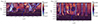Fig. 1. Vertical slices showing the flows from Runs A0 (left) and A100 (right). Note that the box is deeper in the latter case. The colour contours indicate the vertical velocity, uz. The tilde refers to normalisation by $\sqrt{\mathit{dg}}$. The arrows map streamlines where the linewidth reflects the flow speed. The blue and red curves indicate the superadiabatic temperature gradient, Δ∇, with negative (positive) values in blue (red). The boundaries of different zones as defined in Table 1 are indicated by the corresponding labels and orange dotted lines.

Figure 2 shows the energy fluxes from Equations (4) and (5) from Runs A0 and A100. Similar plots for the other runs are shown in Appendix B. A particularly striking result is the increasing depth of the DZ and OZ when n_patch is increased. Table 2 lists the depths of different zones for all of the current simulations. The depth of BZ decreases, and the depth of DZ increases up to n_patch = 100, whereas OZ is already somewhat shallower in Run A50 in comparison to Run A100. In the extreme case of n_patch = 200 (Run A200), the zone structure once more approaches that of Run A0 without cooling patches. The most likely reason is plume merging and the fact that even a small anisotropy in the placing of cooling patches leads to horizontal pressure gradients that can drive large-scale circulation; see Appendix C.

Fig. 2. Horizontally averaged energy fluxes according to Equations (4) and (5), along with ${\overline{F}}_{\text{conv}}$ from runs with npatch = 0 (Run A0, left) and 100 (Run A100, right). The dashed black and white line is proportional to Δ∇.

The last two columns of Table 2 list the depth of the convectively mixed layer, d_mix = d_BZ + d_DZ + d_OZ, and the fraction of d_mix which is stably stratified according to the Schwarzschild criterion, f_mix = (d_DZ + d_OZ)/d_mix. Even in Run A0 with no cooling patches, over 40 per cent of the convectively mixed layer is stably stratified. This fraction increases to 73 per cent in Run A100, in which case only about a quarter of the convectively mixed layer would be considered convective in the classical mixing length paradigm.

The increasing depth of the subadiabatic regions is associated with boosted magnitudes of the convective enthalpy flux, ${\overline{F}}_{\text{enth}}$, and the kinetic energy flux, ${\overline{F}}_{\text{kin}}$. In Runs A50 and A100, the maximum of ${\overline{F}}_{\text{enth}}$ is nearly twice F_bot, and the maximum of $|{\overline{F}}_{\text{kin}}|$ is roughly 1.3F_bot; see Figs. 2 and B1. The latter indicates a significant increase in the energy transport due to downflows. Figure 3 shows the net convected flux (${\overline{F}}_{\text{conv}}$) separately for downflows and upflows for representative runs. In the fiducial Run A0, the upflows and downflows transport roughly equal amounts of flux in the bulk of the CZ between 0.2 ≲ z/d ≲ 0.8. When n_patch increases, the share of the net energy flux carried by the downflows increases such that for n_patch = 50 (Run A50) and n_patch = 100 (Run A100) the upflows contribute only about 0.2F_bot, whereas the downflows transport the majority of the flux with 0.8F_bot. For n_patch = 200, the flux balance more closely resembles the case with no plumes, because large-scale convection ensues in this case; see Figure B1.

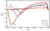Fig. 3. Net convected flux from downflows (${{\overline{F}}_{\text{conv}}}^{\downarrow }$, solid lines) and upflows (${{\overline{F}}_{\text{conv}}}^{\uparrow }$, dashed lines) from representative runs indicated by the legend.

3.2. Spatial scale of convection

The power spectrum of horizontal velocities, E_H(k) at z/d = 0.85, from representative runs are shown in Figure 4. The maximum of E_H(k) is at the largest possible scale irrespective of the boundary forcing. This is likely due to the aforementioned sensitivity to the placement of the cooling patches leading to horizontal pressure gradients that drive flows possibly on very large scales; see Appendix C. This is an issue especially in the cases studied here where the cooling patches are stationary. On intermediate scales (5 ≲ k/k_H ≲ 40), the power spectra for the horizontal flows are close to the Bolgiano-Obukhov k^−11/5 scaling, as in Käpylä (2021) and Warnecke et al. (2025). The peak of the power spectrum of vertical flows, E_V(k), shifts towards smaller scales (higher k) as n_patch increases, reflecting the dominance of the plumes for vertical flows. In Figure 4 normalisation ischosen such that differences between runs appear in the shape of the spectra. An alternative presentation highlighting the absolute differences between runs is shown in Appendix D.

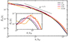Fig. 4. Power spectra of horizontal flows, EH(k), from the same runs as in Figure 3 from z/d = 0.85. Bolgiano-Obukhov k−11/5 scaling is shown for reference. The inset shows the power spectrum of vertical flows, EV(k) for k/kH < 40 for the same runs. Tildes refer to normalisation by the integrated spectrum for each case.

4. Conclusions

The current proof-of-concept simulations show that strong entropy rain can radically change the convective flows and the ensuing energy transport as well as the thermal structure of the convection zone. In the entropy rain-dominated regime, convection is dominated by downflow plumes that penetrate the whole convection zone, rendering the majority of the convectively mixed layer weakly stably stratified, in line with the pioneering ideas of Spruit (1997) and Brandenburg (2016). The idea of entropy rain-dominated convection in the Sun coincides with the recent studies of solar Rossby waves that suggest weak subadiabaticity of the deep convection zone (Bekki 2024) and conjectured fast small-scale downflows at supergranular scales (Hanson et al. 2024). Incorporating entropy rain in global simulations is challenging because the associated small-scaledownflows need to be resolved. An alternative is to include a non-gradient Deardorff term, ${\mathbf{F}}^{\text{SGS}}\propto -\tau \overline{\rho }\overline{T}\mathbf{g}\overline{{s\prime }^2}/c_{\text{P}}$ (Deardorff 1961, 1966), that can capture the non-local transport by plumes in SGS models. Simpler local simulations, such as the current ones, can perhaps be used to constrain such SGS formulations.

The current simulations employ a simple setup and probe a very modest portion of the presently accessible parameter space. Early numerical studies of isolated plumes have indicated a sensitivity to the Prandtl number (Rast 1998), which is also relevant for convection (e.g. Cattaneo et al. 1991; Käpylä 2021). Exploring the dynamics and transport properties of turbulent plumes in astrophysically relevant low Prandtl number regimes is an obvious future direction. Furthermore, rotation and magnetic fields that are dynamically important in stellar interiors are neglected in the current study. Although a recent study (Käpylä 2024a) suggests that convection in the Sun is not strongly rotationally constrained anywhere, its effect is perhaps more subtle in the entropy rain-dominated regime because the slow and spatially larger upflows are much more affected by rotation than the fast and small downflows. The increasing anisotropy between upflows and downflows can also have implications for large-scale magnetic field generation due to convection. A possible outcome is enhanced kinetic helicity production in the upflows, leading to a more vigorous large-scale dynamo. The non-linear backreaction of small-scale magnetic fields on convection (Hotta et al. 2022; Hotta 2025) is another aspect that cannot in general be neglected. Lastly, the apparent lack of large-scale thermal Rossby waves or giant cell convection in the Sun is another facet of the convective conundrum. In the extreme case of entropy rain-dominated convection, the bulk of the convection zone is weakly stably stratified, which can lead to a suppression of thermal Rossby waves. These aspects will be explored further in future studies.

Acknowledgments

I thank the anonymous referee for his/her helpful comments on the manuscript. I acknowledge the stimulating discussions with participants of the Nordita Scientific Program on “Stellar Convection: Modeling, Theory and Observations”, in August and September 2024 in Stockholm. The simulations were performed using the resources granted by the Gauss Center for Supercomputing for the project “Cracking the Convective Conundrum” in the Leibniz Supercomputing Centre’s SuperMUC-NG supercomputer in Garching, Germany.

References

Appendix A: Cooling function

The cooling near the surface is described by two parts

$$\begin{array}{c}\hfill \mathcal{C}={\mathcal{C}}_1+{\mathcal{C}}_2,\end{array}$$(A.1)

where

$$\begin{array}{c}\hfill {\mathcal{C}}_1=\rho c_{\mathrm{P}}\frac{T-T_{\mathrm{cool}}}{{\tau }_{\mathrm{cool}1}}{f}_{\mathrm{cool}}(z,z_{\mathrm{cool}}),\end{array}$$(A.2)

where ${\tau }_{\text{cool1}}=0.2\sqrt{d/g}$ is a cooling time and T_cool = T_top is a reference temperature corresponding to the fixed value at the top boundary. To ensure that the layer above z_cool remains nearly isothermal in the case with n_patch = 0, τ_cool1 ≪ τ_conv is used, where ${\tau }_{\text{conv}}={(u_{\text{rms}}{k}_1)}^{-1}\approx 7\sqrt{d/g}$ is the convective turnover time. Furthermore,

$$\begin{array}{c}\hfill f_{\mathrm{cool}}(z,z_{\mathrm{cool}})=\frac{1}{2}[1+tanh\left(\frac{z-z_{\mathrm{cool}}}{d_{\mathrm{cool}}}\right)],\end{array}$$(A.3)

where z_cool/d = 1 and d_cool = 0.01d.

In addition, n_patch localized cooling patches are introduced via 𝒞₂. Each patch follows:

$$\begin{array}{cc}\hfill {\mathcal{C}}_2& =\rho c_{\mathrm{P}}\frac{T-T_{\mathrm{cool}}}{{\tau }_{\mathrm{cool}2}}{f}_{\mathrm{cool}}(z,z_{\mathrm{patch}})\times \hfill \\ \hfill & exp(-\frac{1}{2}\frac{{(x-x_{\mathrm{patch}})}^2+{(y-y_{\mathrm{patch}})}^2}{d_{\mathrm{patch}}^2}),\hfill \end{array}$$(A.4)

where ${\tau }_{\text{cool2}}=0.067\sqrt{d/g}$, f_cool is the same profile as above with z_patch/d = 0.96, and where the width of the patches is d_patch = 0.05d. Since z_patch < z_cool, the localized cooling corresponds to cool fingers penetrating the upper part of the convection zone. τ_cool2 < τ_cool1 is chosen to ensure that cooling in the patch locations is more effective also for z > z_cool. The number of patches (n_patch) is another input to the models. In the present study the positions (x_patch, y_patch) of the patches are fixed in time and chosen such that ${\displaystyle \sum _i^{n_{\text{patch}}}}{x_{\text{patch}}}^{(i)}=0$ and ${\displaystyle \sum _i^{n_{\text{patch}}}}{y_{\text{patch}}}^{(i)}=0$, except in two control runs used to study the sensitivity of the results to patch placement; see Appendix C.

Appendix B: Energy fluxes

Figure B1 shows the energy fluxes from Runs A10, A20, A50, and A200.

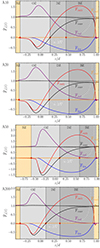Fig. B.1. Horizontally averaged energy fluxes according to Equations (4) and (5) along with ${\overline{F}}_{\text{conv}}$ from runs with nplume = 10 (top), 20, 50, and 200 (bottom).

Appendix C: Sensitivity to patch placement

Large-scale flow generation is possible due to the anisotropic positioning of the cooling patches as alluded to in Section . In the runs listed in Table 2 the patches were initialized at random positions but the positions of some of the patches were adjusted to avoid overlap and large-scale anisotropy; see Appendix A. I refer to this as a semi-optimized set-up. A fully optimized set-up corresponds to a case where the patches are uniformly spaced such that the horizontal anisotropy vanishes. Such a set-up was used in Run A49u, where n_patch = 49 because uniform spacing in 2D requires n_patch = N², where N is an integer. The results from Runs A49u, A50, and two further runs with randomly chosen patch positions with n_patch = 50 (Runs A50r1 and A50r2) are shown in Table C.1 and Figure C1.

Fig. C.1. Same as Figure 4 but for runs listed in Table C.1.

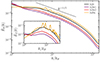
Table C.1 shows that the depth of the BZ remains almost unaffected irrespective of the patch positions. The differences for d_DZ are also relatively minor on the order of 10 per cent. The OZ is significantly reduced in Runs A50r1 and A50r2 with randomly placed cooling patches. The semi-optimized Run A50 and the fully isotropic case A49u are similar in this respect. Figure C1 shows the horizontal and vertical power spectra for the runs in Table C.1. The horizontal flow spectra of Runs A50r1 and A50r2 are similar and have their maxima at the system scale, while in Runs A50 and A49u the horizontal spectrum is flatter at small k, although in the former the maximum still occurs at k/k_H = 1. Furthermore, the vertical flow spectra for Runs A50r1 and A50r2 is much flatter than for Runs A50 and A49u. The latter run again shows the lowest amplitude at the system scale. The differences are explained by the generation of large-scale circulation resulting from the anisotropy of the cooling patches.

Figure C2 shows the flow near the surface of the BZ from Runs A50 and A50r1 along with the positions of the cooling patches. In Run A50 the convection cells are clearly smaller and the horizontal flows are weaker than in Run A50r1. In the latter case clusters of patches as well as voids with no patches appear; see for example regions centered around (x, y) = (−1.5, −0.8)d and (x, y) = (−1.0, 0.5)d for clusters, and the region centered at (x, y) = (0.25, 1.0)d for a large void.

In the Sun the entropy rain is thought to originate from the surface as a consequence of radiative cooling. The solar surface layers are practically unaffected by rotation such that the distribution of downflows is isotropic at the surface. This information can be used to construct a dynamic entropy rain-inducing cooling function that is on average isotropic. This can be achieved, for example, by having cooling patches advected by the mean flow and repulse each other to avoid clustering. Such improvements and generalization to spherical geometry will be considered in future studies.

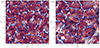Fig. C.2. Vertical velocity uz (colour contours) and horizontal flows (white arrows) near the surface at z/d = 0.85 from Runs A50 (left) and A50r1 (right), averaged over ten snapshots during a time interval of $10\sqrt{d/g}$ or about 1.3τconv. The red circles show the positions of the cooling patches.

Appendix D: Power spectra and anisotropy

The horizontal and vertical velocity power spectra are defined such that

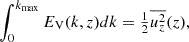$$\begin{array}{cc}\hfill {\displaystyle {\int }_0^{k_{\max }}}{E}_{\mathrm{V}}(k,z)dk& =\frac{1}{2}\overline{u_z^2}(z),\hfill \end{array}$$(D.1)

$$\begin{array}{cc}\hfill {\displaystyle {\int }_0^{k_{\max }}}{E}_{\mathrm{H}}(k,z)dk& =\frac{1}{2}[\overline{u_x^2}(z)+\overline{u_y^2}(z)].\hfill \end{array}$$(D.2)

Figure D1 shows the vertical and horizontal spectra from the same runs as in Figure 4 but normalized with respect to the integrated spectra in Run A0. Both the vertical and horizontal velocities decrease with n_patch. The anisotropy of the flow can be characterized with the vertical spectral anisotropy parameter (Käpylä 2019b):

$$\begin{array}{c}\hfill A_{\mathrm{V}}(k,z)=\frac{E_{\mathrm{H}}(k,z)-2E_{\mathrm{V}}(k,z)}{E_{\mathrm{K}}(k,z)},\end{array}$$(D.3)

where E_K(k, z) = E_H(k, z)+E_V(k, z). The anisotropy parameter is shown in Figure D2 from z/d = 0.49 which is near the middle of the convectively mixed layer. While the anisotropy at large scales is weak irrespective of n_patch, it is significantly enhanced with increasing n_patch at intermediate and small scales (k/k_H ≳ 7). The increased anisotropy parallels the increasing dominance downflows in the energy transport.

A further diagnostic of the asymmetry of convective flows is the filling factor of downflows f^↓, defined via

$$\begin{array}{c}\hfill {\overline{u}}_z=f^{\downarrow }{\overline{u}}_z^{\downarrow }+(1-f^{\downarrow }){\overline{u}}_z^{\uparrow },\end{array}$$(D.4)

where ${\overline{u}}_z^{\downarrow }$ and ${\overline{u}}_z^{\uparrow }$ are the averaged downflows and upflows, respectively. Figure D3 shows that the filling factor decreases monotonically everywhere when more downflow plumes are added until n_patch = 50. This can be understood such that in cases with many plumes, cellular convection is excited only near the surface whereas deeper down the average stratification is stably stratified and plumes are almost the only downflow structures. For n_patch = 100 (Run A100) the spatial profile of f^↓ changes although it is still on average lower than for the cases with fewer plumes. For n_patch = 200 (Run A200) the filling factor is again similar to the cases with few or no imposed plumes. This is explained by merging of plumes already near the surface into larger downflows and the development of large-scale overturning convection in that case.

Fig. D.1. Same as Figure 4 but normalization with respect to the integrated spectra of Run A0.

Fig. D.2. Anisotropy parameter AV(k) from the same runs as in Figure 4.

Fig. D.3. Filling factor of downflows as a function of depth from all of the current runs.

All Tables

All Figures

Fig. 1. Vertical slices showing the flows from Runs A0 (left) and A100 (right). Note that the box is deeper in the latter case. The colour contours indicate the vertical velocity, uz. The tilde refers to normalisation by $\sqrt{\mathit{dg}}$. The arrows map streamlines where the linewidth reflects the flow speed. The blue and red curves indicate the superadiabatic temperature gradient, Δ∇, with negative (positive) values in blue (red). The boundaries of different zones as defined in Table 1 are indicated by the corresponding labels and orange dotted lines.

In the text

	Fig. 2. Horizontally averaged energy fluxes according to Equations (4) and (5), along with ${\overline{F}}_{\text{conv}}$ from runs with npatch = 0 (Run A0, left) and 100 (Run A100, right). The dashed black and white line is proportional to Δ∇.
In the text

	Fig. 3. Net convected flux from downflows (${{\overline{F}}_{\text{conv}}}^{\downarrow }$, solid lines) and upflows (${{\overline{F}}_{\text{conv}}}^{\uparrow }$, dashed lines) from representative runs indicated by the legend.
In the text

	Fig. 4. Power spectra of horizontal flows, EH(k), from the same runs as in Figure 3 from z/d = 0.85. Bolgiano-Obukhov k−11/5 scaling is shown for reference. The inset shows the power spectrum of vertical flows, EV(k) for k/kH < 40 for the same runs. Tildes refer to normalisation by the integrated spectrum for each case.
In the text

	Fig. B.1. Horizontally averaged energy fluxes according to Equations (4) and (5) along with ${\overline{F}}_{\text{conv}}$ from runs with nplume = 10 (top), 20, 50, and 200 (bottom).
In the text

	Fig. C.1. Same as Figure 4 but for runs listed in Table C.1.
In the text

	Fig. C.2. Vertical velocity uz (colour contours) and horizontal flows (white arrows) near the surface at z/d = 0.85 from Runs A50 (left) and A50r1 (right), averaged over ten snapshots during a time interval of $10\sqrt{d/g}$ or about 1.3τconv. The red circles show the positions of the cooling patches.
In the text

	Fig. D.1. Same as Figure 4 but normalization with respect to the integrated spectra of Run A0.
In the text

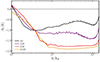	Fig. D.2. Anisotropy parameter AV(k) from the same runs as in Figure 4.
In the text

	Fig. D.3. Filling factor of downflows as a function of depth from all of the current runs.
In the text

References

- Anders, E. H., Lecoanet, D., & Brown, B. P. 2019, ApJ, 884, 65 [NASA ADS] [CrossRef] [Google Scholar]
- Bekki, Y. 2024, A&A, 682, A39 [NASA ADS] [CrossRef] [EDP Sciences] [Google Scholar]
- Bekki, Y., Hotta, H., & Yokoyama, T. 2017, ApJ, 851, 74 [NASA ADS] [CrossRef] [Google Scholar]
- Birch, A. C., Proxauf, B., Duvall, T. L., et al. 2024, Phys. Fluids, 36, 117136 [Google Scholar]
- Brandenburg, A. 2016, ApJ, 832, 6 [Google Scholar]
- Brandenburg, A., Nordlund, A., & Stein, R. F. 2000, in Geophysical and Astrophysical Convection, Contributions from a workshop sponsored by the Geophysical Turbulence Program at the National Center for Atmospheric Research, October, 1995, eds. P. A. Fox, & R. M. Kerr (The Netherlands: Gordon and Breach Science Publishers), 85 [Google Scholar]
- Brandenburg, A., Chan, K. L., Nordlund, Å., & Stein, R. F. 2005, AN, 326, 681 [NASA ADS] [Google Scholar]
- Brun, A. S., Strugarek, A., Noraz, Q., et al. 2022, ApJ, 926, 21 [NASA ADS] [CrossRef] [Google Scholar]
- Cattaneo, F., Brummell, N. H., Toomre, J., Malagoli, A., & Hurlburt, N. E. 1991, ApJ, 370, 282 [CrossRef] [Google Scholar]
- Cossette, J.-F., & Rast, M. P. 2016, ApJ, 829, L17 [Google Scholar]
- Deardorff, J. W. 1961, J. Atmosph. Sci., 18, 540 [NASA ADS] [Google Scholar]
- Deardorff, J. W. 1966, J. Atmosph. Sci., 23, 503 [NASA ADS] [CrossRef] [Google Scholar]
- Dobler, W., Stix, M., & Brandenburg, A. 2006, ApJ, 638, 336 [NASA ADS] [CrossRef] [Google Scholar]
- Edwards, J. M. 1990, MNRAS, 242, 224 [NASA ADS] [CrossRef] [Google Scholar]
- Gizon, L., Cameron, R. H., Bekki, Y., et al. 2021, A&A, 652, L6 [NASA ADS] [CrossRef] [EDP Sciences] [Google Scholar]
- Hanasoge, S. M., Duvall, T. L., Jr., & DeRosa, M. L. 2010, ApJ, 712, L98 [Google Scholar]
- Hanasoge, S. M., Duvall, T. L., & Sreenivasan, K. R. 2012, Proc. Natl. Acad. Sci., 109, 11928 [Google Scholar]
- Hanson, C. S., Bharati Das, S., Mani, P., Hanasoge, S., & Sreenivasan, K. R. 2024, Nat. Astron., 8, 1088 [Google Scholar]
- Hotta, H. 2017, ApJ, 843, 52 [Google Scholar]
- Hotta, H. 2025, ApJ, 985, 163 [Google Scholar]
- Hotta, H., & Kusano, K. 2021, Nat. Astron., 5, 1100 [NASA ADS] [CrossRef] [Google Scholar]
- Hotta, H., Kusano, K., & Shimada, R. 2022, ApJ, 933, 199 [NASA ADS] [CrossRef] [Google Scholar]
- Joyce, M., & Tayar, J. 2023, Galaxies, 11, 75 [NASA ADS] [CrossRef] [Google Scholar]
- Käpylä, P. J. 2019a, A&A, 631, A122 [NASA ADS] [CrossRef] [EDP Sciences] [Google Scholar]
- Käpylä, P. J. 2019b, Astron. Nachr., 340, 744 [CrossRef] [Google Scholar]
- Käpylä, P. J. 2021, A&A, 655, A78 [NASA ADS] [CrossRef] [EDP Sciences] [Google Scholar]
- Käpylä, P. J. 2024a, A&A, 683, A221 [NASA ADS] [CrossRef] [EDP Sciences] [Google Scholar]
- Käpylä, P. J. 2024b, in IAU Symposium, eds. A. V. Getling, & L. L. Kitchatinov, IAU Symposium, 365, 5 [Google Scholar]
- Käpylä, P. J., Korpi, M. J., Stix, M., & Tuominen, I. 2007, in Convection in Astrophysics, eds. F. Kupka, I. Roxburgh, & K. L. Chan, IAU Symposium, 239, 437 [NASA ADS] [Google Scholar]
- Käpylä, P. J., Rheinhardt, M., Brandenburg, A., et al. 2017, ApJ, 845, L23 [CrossRef] [Google Scholar]
- Käpylä, P. J., Browning, M. K., Brun, A. S., Guerrero, G., & Warnecke, J. 2023, Space Sci. Rev., 219, 58 [CrossRef] [Google Scholar]
- Kupka, F., & Muthsam, H. J. 2017, Liv. Rev. Comp. Astrophys., 3, 1 [NASA ADS] [CrossRef] [Google Scholar]
- Nelson, N. J., Featherstone, N. A., Miesch, M. S., & Toomre, J. 2018, ApJ, 859, 117 [Google Scholar]
- O’Mara, B., Miesch, M. S., Featherstone, N. A., & Augustson, K. C. 2016, Adv. Space Res., 58, 1475 [CrossRef] [Google Scholar]
- Pencil Code Collaboration (Brandenburg, A., et al.) 2021, J. Open Source Softw., 6, 2807 [Google Scholar]
- Rast, M. P. 1998, J. Fluid Mech., 369, 125 [Google Scholar]
- Rieutord, M., & Zahn, J. P. 1995, A&A, 296, 127 [Google Scholar]
- Roxburgh, L. W., & Simmons, J. 1993, A&A, 277, 93 [NASA ADS] [Google Scholar]
- Schumacher, J., & Sreenivasan, K. R. 2020, Rev. Mod. Phys., 92, 041001 [NASA ADS] [CrossRef] [Google Scholar]
- Spruit, H. 1997, Mem. Soc. Astron. It., 68, 397 [Google Scholar]
- Stein, R. F., & Nordlund, Å. 1998, ApJ, 499, 914 [Google Scholar]
- Tremblay, P.-E., Ludwig, H.-G., Freytag, B., et al. 2015, ApJ, 799, 142 [Google Scholar]
- Vitense, E. 1953, Z. Astrophys., 32, 135 [NASA ADS] [Google Scholar]
- Warnecke, J., Korpi-Lagg, M. J., Rheinhardt, M., Viviani, M., & Prabhu, A. 2025, A&A, 696, A93 [NASA ADS] [CrossRef] [EDP Sciences] [Google Scholar]
- Weiss, A., Hillebrandt, W., Thomas, H. C., & Ritter, H. 2004, Cox and Giuli’s Principles of Stellar Structure (Cambridge, UK: Cambridge Scientific Publishers Ltd) [Google Scholar]
- Yokoi, N., Masada, Y., & Takiwaki, T. 2022, MNRAS, 516, 2718 [Google Scholar]