| Issue |
A&A
Volume 683, March 2024
|
|
|---|---|---|
| Article Number | A211 | |
| Number of page(s) | 19 | |
| Section | Extragalactic astronomy | |
| DOI | https://doi.org/10.1051/0004-6361/202347596 | |
| Published online | 20 March 2024 | |
At the end of cosmic noon: Short gas depletion times in unobscured quasars at z ∼ 1
1
Leiden Observatory, Leiden University, Niels Bohrweg 2, 2333 CA Leiden, The Netherlands
e-mail: friascastillom@strw.leidenuniv.nl
2
THz Sensing Group, Department of Microelectronics, Faculty of Electrical Engineering, Mathematics and Computer Science, Mekelweg 4, 2628 CD Delft, The Netherlands
3
European Southern Observatory, Karl-Schwarzschild-Straße 2, 85748 Garching bei München, Germany
4
Excellence Cluster ORIGINS, Boltzmannstraße 2, 85748 Garching bei München, Germany
5
Ludwig-Maximilian-Universität, Professor-Huber-Platz 2, 80539 München, Germany
6
School of Mathematics, Statistics and Physics, Newcastle University, Newcastle upon Tyne NE1 7RU, UK
7
ASTRON, Netherlands Institute for Radio Astronomy, Oude Hoogeveensedijk 4, 7991 PD Dwingeloo, The Netherlands
8
Kapteyn Astronomical Institute, University of Groningen, PO Box 800 9700 AV Groningen, The Netherlands
9
South African Radio Astronomy Observatory (SARAO), PO Box 443 Krugersdorp 1740, South Africa
10
Department of Physics, University of Pretoria, Lynnwood Road, Hatfield, Pretoria 0083, South Africa
Received:
28
July
2023
Accepted:
27
December
2023
Unobscured quasars (QSOs) are predicted to be the final stage in the evolutionary sequence from gas–rich mergers to gas–depleted, quenched galaxies. Studies of this population, however, find a high incidence of far–infrared–luminous sources–suggesting significant dust-obscured star formation–but direct observations of the cold molecular gas fuelling this star formation are still necessary. We present a NOEMA study of CO(2–1) emission, tracing the cold molecular gas, in ten lensed z = 1 − 1.5 unobscured QSOs. We detected CO(2–1) in seven of our targets, four of which also show continuum emission (λrest = 1.3 mm). After subtracting the foreground galaxy contribution to the photometry, spectral energy distribution fitting yielded stellar masses of 109 − 11 M⊙, with star formation rates of 25−160 M⊙ yr−1 for the host galaxies. These QSOs have lower LCO′ than star–forming galaxies with the same LIR, and show depletion times spanning a large range (50−900 Myr), but with a median of just 90(αCO/4) Myr. We find molecular gas masses in the range ≤2−40 × 109(αCO/4) M⊙, which suggest gas fractions above ∼50% for most of the targets. Despite the presence of an unobscured QSO, the host galaxies are able to retain significant amounts of cold gas. However, with a median depletion time of ∼90 Myr, the intense burst of star formation taking place in these targets will quickly deplete their molecular gas reservoirs in the absence of gas replenishment, resulting in a quiescent host galaxy. The non–detected QSOs are three of the four radio–loud QSOs in the sample, and their properties indicate that they are likely already transitioning into quiescence. Recent cosmological simulations tend to overestimate the depletion times expected for these z ∼ 1 QSO–host galaxies, which is likely linked to their difficulty producing starbursts across the general high-redshift galaxy population.
Key words: gravitation / gravitational lensing: strong / galaxies: ISM / quasars: emission lines / galaxies: starburst / submillimeter: ISM
© The Authors 2024
 Open Access article, published by EDP Sciences, under the terms of the Creative Commons Attribution License (https://creativecommons.org/licenses/by/4.0), which permits unrestricted use, distribution, and reproduction in any medium, provided the original work is properly cited.
This article is published in open access under the Subscribe to Open model. Subscribe to A&A to support open access publication.
1. Introduction
The nature of massive galaxies changes dramatically between the epoch of the peak star-forming activity of the Universe (z = 1 − 3, “cosmic noon”), and the present day (e.g. Casey et al. 2014). At cosmic noon, the most massive galaxies are typically sub-millimetre galaxies (SMGs) – gas-rich systems with star formation rates (SFR) of 102 − 103 M⊙ yr−1. These are likely progenitors of the z = 0 early type, quiescent galaxies. According to one of the most popular models of massive galaxy evolution, these changes are driven by interactions and mergers of gas–rich SMGs (e.g. Sanders et al. 1988; Alexander et al. 2005; Hopkins et al. 2008; Page et al. 2012; Somerville & Davé 2015). Following the merger, gas is funnelled to the centre of the galaxy through the loss of angular momentum, triggering powerful active galactic nuclei (AGN), accompanied by a starburst (Hopkins et al. 2006). The dusty interstellar medium (ISM) results in an obscured quasar (QSO). Eventually, feedback from the QSO and/or star formation drives the cold gas and dust out of the galaxy through winds and outflows, quenching star formation in the host galaxy and becoming an unobscured QSO. This scenario naturally explains the coevolution of the black hole (BH) and its host galaxy (Kormendy & Ho 2013), which is implied by the observed relation between the mass of the BH and the mass and velocity dispersion of their host spheroids (Ferrarese & Merritt 2000; Gebhardt et al. 2000).
Quasars that are luminous in the far-infrared (FIR) to millimetre regime are thought to be a transition phase between the FIR-bright SMG and FIR-faint, unobscured QSO phases, in which the QSO host galaxies have depleted gas reservoirs but are still able to sustain dust-obscured star formation. The low spatial density of FIR–luminous QSOs, compared to that of SMGs or UV–bright QSOs, previously led some studies to argue that this is a short–lived transition, with timescales as short as 1 Myr (Simpson et al. 2012). Far-infrared studies of QSOs consistently find, however, that they tend to reside in host galaxies with ongoing star formation (e.g. Gürkan et al. 2015; Harris et al. 2016; Netzer et al. 2016), with SFRs similar to those of normal, star-forming (e.g. Rosario et al. 2013; Stanley et al. 2017) or even gas–rich, starbursting galaxies (e.g. Pitchford et al. 2016). A Herschel/SPIRE snapshot imaging survey of all high–redshift lensed QSOs known at the time by Stacey et al. (2018) revealed that ∼70% of QSOs still have significant obscured star formation. This high incidence of an active AGN and high levels of star formation suggests that FIR–luminous QSOs might be able to maintain star formation for longer periods of time, of the order of ∼100 Myr, despite the presence of feedback from ongoing AGN activity.
Studies of the cold ISM in these systems are crucial to understand what drives the high SFRs. Traced by the rotational emission lines of the carbon monoxide molecule (CO), the cold molecular gas is a fundamental ingredient of the ISM of galaxies, as it directly fuels both star formation (Kennicutt 1998; Bigiel et al. 2008) and accretion onto supermassive BHs (see Storchi-Bergmann & Schnorr-Müller 2019, for a review). Results from studies at z ≥ 2 present discrepant findings. Some studies find that QSO host galaxies have lower gas fractions and gas depletion times than their non-QSO counterparts (Kakkad et al. 2017; Perna et al. 2018; Bischetti et al. 2021; Circosta et al. 2021) and interpret this as highly efficient gas consumption due to the AGN feedback affecting the gas. These studies are, however, limited to the most massive and brightest systems due to sensitivity limitations. Other studies of AGN host-galaxies find that they have gas fractions that are indistinguishable from normal star-forming galaxies (SFGs) on the main sequence (Rodighiero et al. 2019; Valentino et al. 2021). In the local Universe, meanwhile, studies find no evidence of the impact of AGN feedback, with the gas reservoirs of AGN–host galaxies showing similar properties to those of SFGs (Husemann et al. 2017; Rosario et al. 2018; Jarvis et al. 2020; Shangguan et al. 2020a; Yesuf & Ho 2020; Koss et al. 2021; Zhuang et al. 2021).
The redshift 1 < z < 1.5 corresponds to the end of the peak epoch of both star formation and accretion activity of BHs (Shankar et al. 2009; Madau & Dickinson 2014), and is therefore a crucial laboratory to look for AGN feedback effects. There is little direct knowledge (via CO observations) of the molecular gas reservoirs in FIR–luminous QSOs at this redshift range, right at the end of cosmic noon, when the energy input into the host galaxy from the AGN might be maximised. Previous work at z = 1 − 1.5 was undertaken as part of a larger CO survey of 18 gravitationally lensed QSOs in the redshift range ∼1.3−3.8 by Barvainis et al. (2002), who obtained only upper limits at z ∼ 1.5. To date, there have only been two CO detections of unobscured, FIR–bright QSOs, which should be about to enter the quenched phase of their evolutionary path. These are the lensed Q 0957+561 (Krips et al. 2005) and HS 0810+2554 (Chartas et al. 2020; Stacey et al. 2021), which have molecular gas masses of ≃1010 and ≃3−5 × 10⁹ M⊙, respectively, with estimated depletion times of ≃100 Myr. At a slightly lower redshift, however, the strongly lensed QSO RXJ1131−1231 (z ∼ 0.65) has a massive (∼1011 M⊙) molecular gas disc ∼15 kpc in diameter (Paraficz et al. 2018), with a depletion time of 1 Gyr, more typical of normal SFGs (Tacconi et al. 2018). The large difference in molecular gas mass and depletion times suggests a large scatter in cold gas content among unobscured QSOs at z ∼ 1 − 1.5.
Motivated by these findings, we have targeted the CO(2–1) (νrest = 230.5380 GHz) emission line in a sample of strongly lensed unobscured QSOs in the redshift range z = 1 − 1.5 using the NOrthern Extended Millimitre Array (NOEMA). These are all the QSOs in this redshift range which are detected in targeted Herschel SPIRE photometry from the survey by Stacey et al. (2018) and that are observable by NOEMA. By targeting gravitationally lensed objects, we probe fainter systems that would otherwise need prohibitively long integration times to be detected, although this comes at the expense of differential magnification effects. This survey aims to study the gas content in these intermediate–redshift QSOs, establishing their gas depletion times and gas fractions. With this data, we aim to fit these QSOs in the canonical SMG-QSO evolution scenario. Specifically, we aim to answer the question of whether their gas reservoirs are massive enough to maintain their obscured SFRs for long periods of time, or they are about to be quenched.
The paper is structured as follows. In Sect. 2 we describe the sample selection, NOEMA observations, and data reduction. In Sect. 3, we present the CO(2–1) line and continuum detections, a search for the HCN/HNC/HCO+ lines covered by our observations, and we describe our SED fitting approach. In Sect. 4 we analyse the  relation for the sample (Sect. 4.2), their total cold molecular gas content (Sect. 4.3), gas fractions and depletion times (Sect. 4.4), and compare our results with different studies from the literature, as well as state-of-the-art simulations (Sect. 4.5). Finally, we present our conclusions in Sect. 6. Throughout this paper, we adopt a flat universe model with a Hubble constant of H0 = 67.8 km s−1 Mpc−1, ΩM = 0.31, and ΩΛ = 0.69 (Planck Collaboration XIII 2016).
2. Observations and data reduction
2.1. Target sample
Our targets are drawn from the sample of 104 gravitationally lensed QSOs observed with the Herschel Space Observatory (Pilbratt et al. 2010) using the Spectral and Photometric Imaging Receiver (SPIRE) instrument (Griffin et al. 2010). We refer the reader to Stacey et al. (2018) for further details on the selection of the parent sample. From this list of targets, we selected all QSOs detected in FIR with known redshifts within the range z = 1 − 1.5 for which the CO(2–1) emission line is observable with NOEMA. Three of our sources, B1608+656, B1152+200, and B1600+434, have strong jet–dominated radio emission (Browne et al. 2003).
The final sample is shown in Table 1. The magnification factors listed have been derived from high-resolution observations in the FIR to sub-millimetre regime. When no magnification has been derived for a source, we assume a magnification of  for the intrinsic properties discussed throughout the paper and propagate the errors accordingly. We note that the bulk of our analysis is based on brightness ratios and thus independent of the magnification factor.
Target sample, ordered by increasing source redshift.
A different source-plane distribution of the dust (FIR), gas (CO), and stellar emission might however result in a differential magnification bias – that is, each tracer is magnified by a different factor. These can be significant, especially in highly magnified systems – for example, in the strongly lensed AGN host B1938+666, the FIR and CO(1–0) emission are magnified by a factor of ≈16 and ≈9, respectively (Spingola et al. 2020). While our spatially unresolved CO(2–1) observations do not allow us to derive the corresponding magnifications via lens modelling, we do not expect significant differential magnification bias in our sample. First, out of the seven sources detected in CO(2–1), five are doubly imaged, which reduces the differential magnification. Second, even in quadruply lensed systems such as SDP.81, the difference between FIR continuum and CO magnifications is ≤20% (Rybak et al. 2020), comparable to other uncertainties in our analysis (such as relative flux calibration). Therefore, we do not expect differential magnification to affect the main conclusions of this paper. Future resolved CO(2–1) and (sub)mm-wave imaging will be necessary to derive proper magnification factors for each component.
2.2. NOEMA observations and data reduction
The observations were conducted as a part of the NOEMA projects S19CC and W20CM (PI: M. Rybak) between 2019 June 8 and 2020 December 30 in Band 1 in D configuration, with nine to ten 15-m antennas. The details of the observations are summarised in Table A.1. The water vapour (pwv) estimates are based on the 22-GHz radiometer measurements. At our targeted frequency (100 GHz), the primary beam has a full width at half-maximum (FWHM) of ∼50 arcsec. We used the PolyFiX correlator with a standard spectral resolution of 2 MHz to cover a total bandwidth of 15 GHz.
The observations were tuned to centre the CO(2–1) transition of each source in the upper sideband. Depending on the target and time of observation, one of the two strong radio stars MWC349 or LKHA101 were observed for absolute flux calibration. For bandpass calibration, we used either 3C84, 3C279, 3C345, 1055+018, 1633+382, 1749+428 or 2013+370, depending on the target and time of observation. We integrated between 2.2 and 10.8 h on each source, resulting in a noise level in the range of 0.2−0.5 mJy beam−1 at a spectral resolution of 20 MHz using natural weighting. The final integrated beam sizes and sensitivities are reported in Table 2.
NOEMA imaging: final synthesised beam sizes and sensitivity for the integrated continuum (given at 1.3 mm rest-frame) and 20 MHz bandwidth at the position of the CO(2–1) line (∼60 km s−1), for natural weighting.
Data calibration, cleaning, and imaging was carried out using the GILDAS CLIC software package1. We selected channels on both sides of the CO(2–1) emission line as the fitting windows of linear baselines and subtracted a zeroth-order baseline from the cubes in the image plane to remove any continuum emission. We then imaged the residual spectral-line visibilities at spectral resolutions of 2−50 MHz. Finally, we also created maps of the 3 mm continuum emission after masking channels where the CO(2–1) line was detected. With the angular resolution achieved in this configuration (Table 2), the targets are marginally resolved.
For B1608+656, B1152+200, and B1600+434, we used the very strong continuum signal (S/N > 100) to self-calibrate the data, solving for the phase only. No CO(2–1) emission was detected before or after the self-calibration.
3. Results
3.1. CO(2–1) line
To determine the flux and FWHM of the CO(2–1) line, we proceeded as follows. For each target, we considered the continuum-subtracted cube and extracted a line spectrum using a beam-sized aperture placed on the central pixel. The extracted spectrum was then fit with a one-dimensional Gaussian to determine the line centroid, zCO, and FWHM. We used the task IMMOMENTS in CASA (McMullin et al. 2007) to create moment 0 maps by collapsing the spectral channels around the line centroid over a velocity range twice the CO(2–1) line FWHM for each target. The rms of the collapsed maps was estimated over an area approximately half that of the primary beam. We detected the CO(2–1) line in seven out of ten sources (Fig. 1). Since not all our sources showed Gaussian profiles and their emission was extended beyond a beam, we extracted total line fluxes from the moment 0 maps instead of the Gaussian line fits to ensure we recovered all the flux. We did not find evidence of broad and/or asymmetric wings in the CO spectra that could indicate cold gas outflows.
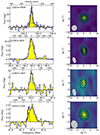 |
Fig. 1. CO(2–1) spectra and 0th moment maps for the detected QSOs. The black solid line indicates the best fit Gaussian model, and the reference velocity was determined based on the redshift derived from the Gaussian fit (LSRK frame). Contours in the 0th moment maps start at 4σ and increase in steps of 4σ for J1524+2209, J1330+1810, J0924+0219, and J1650+4251; contours for J1455+1447, J1633+3134, and J0806+2006 start at 2σ and increase in steps of 2σ. We have used the AIC criterion to determine whether a single- or double–Gaussian fit is more appropriate for the profiles. |
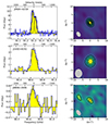 |
Fig. 1. continued. |
To determine the optimal mask for extraction of the line flux, we performed a curve of growth analysis. We iteratively extracted the flux from a circular aperture increased by 1″ at a time, until the extracted flux converged. We found that the flux was extended out to a radius of approximately 6″, so we chose this as the aperture radius to measure the final line fluxes. The line fluxes were consistent with those obtained if we fit a 2D Gaussian to the detected emission. For the sources without a CO detection, we provide a 3σ upper limit, calculated from the rms of the velocity-integrated maps collapsed over a line width of 245 km s−1, the median FWHM measured for our detections. The results of our analysis are reported in Table 3. We measured integrated flux densities of the CO(2–1) line in the range < 0.01−0.28 Jy km s−1 (corrected for magnification) and FWHM in the range 65−550 km s−1.
Line and continuum detections.
3.2. Rest-frame 1.3-mm continuum
We detected continuum emission in 5 of the 10 targets; two more targets showed tentative ∼2σ emission and three were undetected (see Fig. 2). The continuum emission was unresolved, and this was confirmed by a curve of growth analysis which showed that the continuum emission was more compact than that of the CO line. Therefore, we extracted the flux, Scont, from an aperture with a diameter twice that of the beam FWHM, to ensure we recovered all the flux. The continuum fluxes are reported in Table 3, corrected for magnification. We found a good agreement between Scont and the flux density values estimated by fitting a two–dimensional Gaussian model to the continuum image (Fig. 2). Two of our sources had already been observed at this same frequency during the survey carried out by Barvainis et al. (2002) with the Plateau de Bure Interferometer, which gave us the opportunity to assess if the measured fluxes have varied, possibly induced by variable AGN activity. The flux densities quoted below were uncorrected for magnification.
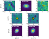 |
Fig. 2. Detected continuum emission at the position of the CO(2–1) emission line for the sample presented in this work. Contours for J1524+4409, J1330+1810, J1633+3134, and J1650+4251 start at ±2σ and increase in intervals of ±1σ, where σ is given in Table 2. Contours are given in steps of ±50σ starting at 50σ for B1608 and in steps of ±100σ starting at 100σ for B1152 and B1600. The red cross indicates the peak position of the gas emission where detected, and the optical emission for the three QSOs not detected in CO(2–1). |
B1608+656: this QSO at z = 1.394 has a continuum flux of 18.4 ± 0.7 mJy at 94 GHz and 16.0 ± 0.7 mJy at 110 GHz, a factor of two larger than the value of 8.1 ± 0.4 mJy reported by Barvainis et al. (2002).
B1600+434: this QSO at z = 1.589 has a continuum flux of 34.3 ± 0.1 mJy at 89 GHz and 31.1 ± 0.1 mJy at 104 GHz, compared to the value of 25 ± 0.3 mJy reported by Barvainis et al. (2002).
These two sources, together with B1152+200, are QSOs with strong radio emission (Stacey et al. 2018). It is thus likely that the 1.3 mm continuum detected with NOEMA is also associated with synchrotron emission coming from the jets.
3.3. Upper limits on outflow flux
We inspected the continuum–subtracted data cubes to search for high–velocity line emission that might be originating from outflows in the sources with detected CO(2–1) emission. We did not find any significant (> 3σ) emission in any of the high–velocity channels that did not contain emission from the main galaxy (beyond ±400 km s−1). To place an upper limit on the total flux, we created intensity maps by collapsing the velocity channels from +500 km s−1 to +1000 km s−1 and from −500 km s−1 to −1000 km s−1, a range commonly adopted when searching for outflow emission in previous works (Cicone et al. 2014; Lutz et al. 2020; Bischetti et al. 2019). We used the same circular aperture of 6″ radius centred on the CO(2–1) emission to extract the flux. This ensured that we were at least covering the area where CO emission was detected, placing conservative upper limits on the mass outflow rates (see Sect. 4.3). We did not detect > 2σ emission in any of the targets. We note that, using the AIC criterion, a double Gaussian was preferred to fit the spectrum of J1524+4409, in a configuration that is often indicative of an outflow. However, it is not unusual to find asymmetric line profiles in lensed sources due to differential magnification of different velocity components (Butler et al. 2023), so we cannot currently confirm the presence of an outflow in this source.
3.4. Spectral energy distribution decomposition
To derive the intrinsic properties of the QSO host galaxies, we used multi-wavelength spectral energy distribution (SED) modelling. Specifically, we included ultraviolet to mm-wave photometry2 available in the literature and via the NASA NED database. As the listed uncertainties are likely to be underestimated due to the use of different apertures, flux calibration uncertainties or confusion limits, for example, we added a 10% error in quadrature to the photometry.
The main challenge in SED modelling of these multi-wavelength datasets is that at most wavelengths, the low spatial resolution of the data causes the blending of the foreground (lensing) galaxy (SFG(λ)) with the background AGN (SAGN(λ)) and host galaxy itself (SBG(λ)):

To decompose these three components, we use a three-step approach:
-
We used resolved imaging (mostly at optical/near–IR wavelengths) to separate the light from the foreground galaxy.
-
We fit the light from the foreground galaxy using the (Brown et al. 2014) templates of nearby galaxies (spanning rest-frame UV to MIR wavelength for a broad range of galaxy types, including ellipticals, spirals, merging galaxies, blue compact dwarfs, and luminous infrared galaxies) and subtracted these from the total SED. This removed the SFG component from the data. We note that the templates used did not extend out to MIR and FIR data. All the lensing galaxies in our sample, with the exception of the lens of B1600+434, are ellipticals with little or no star formation left, and so we did not expect them to have a significant contribution to the total FIR emission. For B1600+434, we used the available SPIRE photometry for UGC 12150, NGC 5104, NGC 5033, and NGC 4594, four of the best fitting spiral templates from the (Brown et al. 2014) catalogue, to extend the average subtracted model and account for the extra FIR emission.
-
We model the remaining μ(SAGN(λ)+SBG(λ)) SED using AGNFITTER, a publicly available SED-modelling package specifically designed to model the SEDs of galaxies with prominent AGNs (Calistro Rivera et al. 2016). The photometry is fitted with a combination of a stellar component, an optical and an infrared AGN component and a FIR component associated with dust-obscured star formation in the host galaxy3. We used the spectroscopic redshifts derived from fitting the CO(2–1) emission lines as input where available. We refer the reader to Calistro Rivera et al. (2016) for a detailed description of the algorithm and templates used.
We derived bolometric and infrared luminosities, stellar masses and IR-based SFRs from SED fitting. The results are summarised in Table 4, and the SED fits are shown in Appendix B. Following Calistro Rivera et al. (2021), we calculated bolometric luminosities Lbol by integrating the emission from the accretion disc component (BBB) over the wavelength range 0.05–1 μm, with an added correction factor of Δlog(Lbol) = 0.3 to account for X-ray emission. The inferred Lbol are consistent with those derived from the 3000 Å luminosity (Rakshit et al. 2020)4. The infrared luminosity, LIR, was calculated by integrating the galaxy cold dust emission over the wavelength range 8–1000 μm after subtracting the AGN contribution to the emission (e.g. Mullaney et al. 2011; Del Moro et al. 2013; Delvecchio et al. 2014). The infrared luminosities obtained are comparable to those derived by Stacey et al. (2018; after correcting for LIR = 1.91 LFIR) for the QSOs with CO detections, with a median ratio of 1.0 ± 0.2 between both values. The QSOs not detected in CO show a larger discrepancy, with the AGNFITTER–derived infrared luminosities being on average ∼40% lower than calculated by Stacey et al. (2018). We note that the available photometry for the QSOs does not currently sample the peak of the IR SED. This is evidenced by the large range of possible luminosities covered by the AGNFITTER models (green component, Figs. B.1 and B.2).
Parameters derived for the sample of unobscured QSOs in this work.
In order to derive the SFR from the starburst model component dominating the FIR, we follow Murphy et al. (2011):
![$$ \begin{aligned} \mathrm{SFR}\,[{M_\odot \,\mathrm{yr}^{-1}}] = 10^{-10} \times {L_{\rm IR} \ [L_\odot ]}, \end{aligned} $$](/articles/aa/full_html/2024/03/aa47596-23/aa47596-23-eq83.gif)
corrected to a Chabrier initial mass function (Chabrier 2003). This does not account for unobscured star formation, so it should be considered as a lower limit. The large uncertainties in the stellar masses reflect the difficulty in separating the optical emission from the stellar population and the QSO in the lensed galaxy. To test the robustness of the stellar masses, we re–ran AGNFITTER without deblending the emission from the foreground and background galaxies (that is, we assumed that all light was associated with the background galaxy). We found that the stellar masses are consistent within a factor of 2. Finally, we used the BH masses (MBH) derived from SDSS spectroscopic observations of the MgII emission line (Rakshit et al. 2020) and the MBH − M* scaling relation from Ding et al. (2020) to calculate the expected values for the stellar mass. The median ratio between the SED- and MBH-derived stellar masses is 1.05, with a mean ratio of 3.8.
3.5. Spectral stacking – Upper limits on dense-gas tracers
Our spectral setup covers several other emission lines, notably HCN(3–2), HCO+(3–2) and HNC(3–2). As none of the lines was detected in individual spectra, we resorted to spectral stacking, following the same procedure as in Rybak et al. (2022): (1): first, we shifted the spectra in frequency to a common redshift z = 1.25; (2) we scaled the observed flux densities to match the luminosity distance at z = 1.25; (3) we took a weighted mean using  weighting. Figure 3 shows the resulting rest-frame stacked spectrum, normalised to a LFIR = 5 × 10¹² L⊙. We did not see any excess line emission, independent of the choice of weighting and spectral binning.
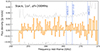 |
Fig. 3. Stacked spectrum of our NOEMA observations over the region covering the HCN/HCO+/HNC(3–2) lines. The spectrum was scaled to an apparent FIR luminosity LFIR = 5 × 10¹² L⊙. We did not find any line detected at ≥3σ significance, indicated by the dashed horizontal line. |
Based on the stacked spectrum, we inferred the following 3σ upper limits on the line vs FIR luminosity ratios:  K km s−1 pc2/L⊙,
  K km s−1 pc2/L⊙,
  K km s−1 pc2/L⊙. These are consistent with the ratios observed in local (ultra) luminous infrared galaxies (e.g. Li et al. 2020).
4. Analysis
To investigate the physical properties of our sample, we compile the following QSOs with observations of molecular gas from the literature for comparison: Q 0957+561 and HS 0810+2554, the only z ∼ 1.5 unobscured QSOs with CO line emission detections in the literature (Krips et al. 2005; Chartas et al. 2020); 34 unobscured QSOs at z = 1.3 − 6.7 and 47 obscured QSOs at z = 1.1 − 6.4 from the compilation by Perna et al. (2018); seven X-ray selected QSOs at z ∼ 2 drawn from SUPER (SINFONI Survey for Unveiling the Physics and Effect of Radiative feedback), which have a reliable measure of LIR (Circosta et al. 2021); seven unobscured QSOs (bolometric luminosity Lbol > 3 × 1047 erg s−2) from the WISE-SDSS selected hyper-luminous (WISSH) QSOs sample at z ∼ 2.4 − 4.7 from Bischetti et al. (2021); 23 z < 0.1 Palomar–Green QSOS from Shangguan et al. (2020b). Finally, we include a sample of 17 SMGs from the AS2COSMOS, AS2UDS and AEGIS surveys presented by Frias Castillo et al. (2023) and 16 SFGs at 1 < z < 3 detected in CO emission with the ASPECS programme (Boogaard et al. 2020). The stellar masses and SFRs for these samples were uniformly obtained through SED fitting with MAGPHYS (da Cunha et al. 2008, 2015).
Where necessary, the reported quantities have been corrected for magnification. In order to homogenise the data, we correct the gas masses associated with the QSOs for αCO = 4. For the SMGs, the most recent studies suggest αCO = 1 is more appropriate given the physical properties of their ISM (Birkin et al. 2021), so we calculate their corresponding total gas masses according to this value. For a more detailed discussion on the adopted αCO, see Sect. 4.3.
The unobscured QSOs targeted by this work were originally drawn from a variety of surveys at optical and radio wavelengths, making it hard to identify and quantify the selection effects biasing the derived properties. However, although small, our sample comprises half of all the lensed QSOs in the z = 1 − 1.5 range from the parent sample in Stacey et al. (2018), with the other half being Herschel–faint sources with no indication of significant ongoing star formation. Therefore, it is likely that our sources are representative of the star–forming unobscured QSO population at this epoch.
4.1. Unobscured QSOs on the SFR–M* plane
Normal star–forming galaxies have been shown to follow a tight correlation between their star formation rates and stellar masses, known as the “star–forming main–sequence (MS)”, which evolves with redshift (e.g. Noeske et al. 2007; Elbaz et al. 2011; Speagle et al. 2014; Schreiber et al. 2015; Leslie et al. 2020). Here, we consider where our targets and the comparison samples lie in relation to the MS as parameterised by Speagle et al. (2014) at z = 1.25. The positions of all the literature samples have been scaled to a common redshift of z = 1.25. Since the MS evolves with redshift, this scaling is necessary to avoid higher–redshift sources appearing like starbursts when placed on the lower–redshift MS relation. It is done by plotting each source on the z = 1.25 MS at the same ΔMS that it would have at its true redshift, where ΔMS is the ratio of its measured SFR compared to that of the main sequence at its redshift and stellar mass, ΔMS = SFR/SFRMS(z, M*). Following the literature (e.g. Rodighiero et al. 2011), we classify a galaxy as a starburst if it lies ΔMS > 0.6 dex above the main sequence.
We show the distribution of our targets on the SFR–M* plot in Fig. 4. Six of our targets have high SFRs and are classified as starbursts following the above definition. The IR–based SFRs are in the range 25−160 M⊙ yr−1, with a median of ∼75 M⊙ yr−1. For comparison, Stanley et al. (2017) and Symeonidis et al. (2022) find IR–based SFRs of 25−120 and ∼60 M⊙ yr−1 for 0.8 < z < 1.5 and z = 1.5 optically selected QSOs, respectively. The SFRs are also consistent with those of the ASPECS SFGs at the same redshift. Therefore, our QSOs do not appear to be exceptional in terms of SFRs compared to other systems at similar redshifts. These results support the consensus that star formation can co–exist with AGN activity, and any significant suppression of star formation due to negative feedback effects must occur on longer timescales (Floyd et al. 2013; Stacey et al. 2018; Rodighiero et al. 2019; Carraro et al. 2020; Jarvis et al. 2020).
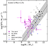 |
Fig. 4. SFR as a function of stellar mass for our sample of unobscured QSOs. The values were obtained through SED fitting with AGNFITTER. For comparison, we have plotted the low–redshift Palomar–Green QSOs from Shangguan et al. (2020b) (grey), high–redshift obscured QSOs (grey, empty circles) from the compilation presented in Perna et al. (2018), a sample of high–redshift SMGs (black stars) and z = 1 − 3 SFGs from ASPECS (blue crosses, Boogaard et al. 2020). The dashed black line marks the main–sequence at z = 1.5 as parameterised by Speagle et al. (2014), with the one sigma scatter shown by the shaded grey area. All data points have been scaled to z = 1.25 for comparison and corrected for magnification where necessary. Most of our targets lie on or above the main–sequence. Their stellar masses are lower than most of the higher–redshift obscured QSOs, but comparable to low–redshift unobscured QSOs and the ASPECS SFGs. |
The stellar masses, with a mean of M* = 2 × 10⁹ M⊙, are consistent with the ASPECS SFGs and low–redshift PG unobscured QSOs, but are on average an order of magnitude lower than those of high–redshift obscured QSOs and SMGs. This could be due to gravitational lensing bias – since the SMGs and obscured QSOs are not lensed, we are biased towards galaxies that are massive and bright enough to be above the detection limits of the different studies. Gravitational lensing allows us to pick up less massive systems that would otherwise be below the detection threshold. We find specific SFRs (sSFR = SFR/M*) in the range log(sSFR) = −6.7 to −9.6, with a median log(sSFR) of −8.1.
4.2.  versus LIR
We derive CO(2–1) line luminosities following Solomon & Vanden Bout (2005):

where ICO is the integrated line flux from the 0th-moment map in Jy km s−1, νobs is the observed frequency in GHz and DL is the luminosity distance in Mpc. In order to derive the CO(1–0) line luminosities, we assume an excitation correction factor,  (Kirkpatrick et al. 2019).
Figure 5 (left) shows the integrated CO luminosities of our targets and the comparison samples as a function of LIR, where the latter has been corrected for AGN contamination. We show the best–fit relation derived for main–sequence galaxies at 0 < z < 3 by Sargent et al. (2014). Both luminosities have been shown to correlate strongly at both high and low redshift (Sanders & Mirabel 1985; Solomon & Vanden Bout 2005; Genzel et al. 2010; Saintonge et al. 2011; Carilli & Walter 2013). Previous studies at z ≥ 2 have found that, while both luminosities are also correlated for QSOs, these appear to be deficient in CO luminosity for a given IR luminosity compared to normal, star–forming galaxies (e.g. Kirkpatrick et al. 2019, but see Perna et al. 2018; Bischetti et al. 2021; Circosta et al. 2021). Our QSOs show intermediate  and LIR compared to their high- and low–redshift counterparts. J1524+4409 and J0924+0219 are consistent with the Sargent et al. (2014) relation for star–forming galaxies, while five of them have lower
  values than the relation would predict for their LIR, in line with other high–redshift QSO studies. It is possible that the QSOs follow instead the relation found for starbursts, rather than main–sequence galaxies (approximately a factor of 3 below the locus of MS galaxies; Sargent et al. 2014). J1650+4251 is consistent with the relation for starbursts, but the remaining four detections and three non–detections still fall below the relation. This deficit in CO luminosity compared to IR luminosity has been suggested as a possible sign of AGN feedback, which would shut off star formation by either depleting the gas present in the host galaxy (Perna et al. 2018; Bischetti et al. 2021) and/or heating up the cold gas through the injection of energy and momentum via outflows.
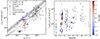 |
Fig. 5. Left: CO(1–0) line luminosity versus infrared luminosity integrated over 8−1000 μm for our sample of unobscured QSOs, coloured as a function of offset from the MS. The CO(1–0) luminosities have been calculated using r21 = 0.86 (Kirkpatrick et al. 2019), and LIR has been corrected for AGN contamination. For comparison, we have plotted the low–redshift Palomar–Green QSOs from Shangguan et al. (2020b), high–redshift obscured (filled grey circles) and unobscured (open grey circles) QSOs from the compilation presented in Perna et al. (2018), a sample of high–redshift SMGs (black stars) and z = 1 − 3 SFGs from ASPECS (Boogaard et al. 2020, blue crosses). Where necessary, all quantities have been corrected for magnification. The black solid and dashed lines show the |


The three non–detected QSOs also have a large offset from the  relation, as well as the lowest offset from the main–sequence (B1152+656 can be classified as quiescent). This combination of low gas mass and star formation rate could be explained if the host galaxies are at the end of the blowout phase, where the molecular gas has been depleted by either QSO or star formation feedback and they are now entering the quenched, post–starburst phase. Theoretical models and observations of nearby galaxies have also shown X-ray irradiation from the central AGN to dissociate CO molecules (e.g. Maloney et al. 1996; Izumi et al. 2020), enhancing the abundance of carbon atoms and further contributing to the CO deficit, but observations of atomic carbon or CO isotopologues would be needed to explore this scenario.
As the IR luminosity is a tracer for star formation, the ratio between  and LIR serves as a proxy for star formation efficiency, usually defined as SFE = SFR/Mgas in units of yr−1. We show this ratio for our sample in Fig. 5 (right). Our QSOs show SFE ratios in the range 30−560 L⊙/(K km s−1 pc2), with a median of 350 L⊙/(K km s−1 pc2). This is similar to the SFE of most high–redshift QSOs and SMGs, but elevated compared to the ASPECS SFGs (median ∼60 L⊙/(K km s−1 pc2)) or the low-z PG QSOs (median ∼50 L⊙/(K km s−1 pc2)). There is likely not a single cause for the high SFE, as it is governed by the balance between the warm and cold HI phases, H2 formation, and perhaps shocks and turbulent fluctuations driven by stellar and AGN feedback. If these QSOs are indeed the last stage of a merger between two gas–rich galaxies, as galaxy evolution models predict, there are also extra factors that have been shown to affect the efficiency of star formation, such as the strength of the torques during the later stages of the merger or the geometry of the collision (Di Matteo et al. 2007; Somerville et al. 2008). It is also possible that there is an increased amount of dense gas available in the QSOs, as a consequence of either the merger or AGN and stellar feedback. Higher-resolution, multi-wavelength data would allow us to better constrain the physical conditions driving the high SFE in these unobscured QSOs.
4.3.  and gas masses
In order to calculate the CO(1–0) line luminosities and derive total cold molecular gas masses from them, it is necessary to assume an excitation correction factor,  , and a conversion factor,
  . For the excitation correction, we assume r21 = 0.86 (Kirkpatrick et al. 2019). The conversion factor αCO introduces the largest uncertainty when calculating gas masses, as it has been shown to be dependent on physical parameters such as metallicity, cloud density and temperature (Bolatto et al. 2013; Accurso et al. 2017). When there are no estimates of these parameters, however, the standard approach is to use either a Milky Way–like value of ∼4 M⊙/(K km s−1 pc2) for normal star–forming galaxies, or a starburst–like factor of 0.8 M⊙/(K km s−1 pc2) for highly star–forming or interacting galaxies (e.g. Brusa et al. 2018; Perna et al. 2018).
The standard approach in previous studies of molecular gas in QSOs has been to assume αCO = 0.8, justified by the fact that many have been found to have compact disc sizes (Brusa et al. 2018; Feruglio et al. 2018), high molecular gas excitation (e.g. Wang et al. 2016) and reside in highly star-forming host galaxies (Carilli & Walter 2013; Combes 2018). However, this might be biased by the fact that we have so far been limited to the most luminous QSOs at high redshift, and conditions affecting the value of αCO might evolve at lower redshifts. Indeed, Paraficz et al. (2018) derived αCO = 5.5 ± 2.0 from resolved CO(2–1) observations for the z = 0.65 QSO RXJ1131–1231, and Shangguan et al. (2020b) found that αCO ∼ 3 is more appropriate for the low–redshift unobscured Palomar Green QSOs. This suggests that αCO = 0.8 might be too low a value to use for our sample. Dunne et al. (2022) recently found αCO = 4 M⊙ (K km s−1 pc2)−1 based on the analysis of a sample of 407 galaxies ranging from local galaxies to high–redshift SMGs spanning up to z ∼ 6, so we assume this value for the purposes of the discussion. If we chose αCO = 0.8 instead and a steeper CO SLED (e.g. r21 = 0.99; Carilli & Walter 2013), the derived gas masses would be reduced by a factor of ∼6. In order to perform a uniform comparison and minimise systematic uncertainties, we calculate molecular gas masses using the same αCO = 4 for all QSOs from the literature samples.
The CO(1–0) luminosities of our sample are shown as a function of redshift in Fig. 6. We obtain line luminosities in the range  × 109 K km s−1 pc2, corrected for magnification, with a median of
  × 109 K km s−1 pc2, corresponding to total cold molecular gas masses in the range Mgas ≤ 2 − 40 × 109 M⊙. Our sample of unobscured QSOs has therefore lower CO luminosities, and gas masses, than those of main–sequence galaxies and other obscured QSOs at similar redshift, but they are comparable to the most luminous QSOs in the local universe (for example, Palomar Green QSOs, Shangguan et al. 2020b). It is possible that, following the canonical galaxy evolutionary models, our unobscured QSOs are in a later evolutionary stage than obscured QSOs at similar redshifts, shown by their more depleted gas reservoirs. However, since the stellar masses are also lower than those of obscured QSOs (Fig. 4), we could also be probing a younger and/or less massive population of QSOs that is not evolutionary connected to the more luminous, high-z counterparts studied so far. This could be an example of “galaxy down–sizing” (Cowie et al. 1996; Fontanot et al. 2009; Mortlock et al. 2011), where more massive galaxies form their stars earlier and over a shorter period of time than lower–mass galaxies. Naturally, if the massive, high–redshift QSOs have exhausted their molecular gas reservoirs and quenched their star formation by z ∼ 1.5, they would have fallen below the detection threshold of the Herschel survey (Stacey et al. 2018).
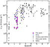 |
Fig. 6. CO(1–0) line luminosities as a function of redshift for our sample. In some cases, error bars are smaller than the marker. The comparison samples are described in Fig. 5. Where necessary, all quantities have been corrected for magnification. On average, the unobscured QSOs targeted in this study have lower CO luminosities than other obscured QSOs and star–forming galaxies at similar redshift. It is thanks to gravitational lensing that we are able to detect these systems with short exposure times. |
Finally, we can place conservative upper limits on the mass outflow rates of these QSOs based on the measured flux at ±500−1000 km s−1. Assuming a simple spherical geometry uniformly populated with the outflowing clouds, the mass outflow rate can be calculated using (Maiolino et al. 2012; Cicone et al. 2014):
where we take v = 1000 km s−1 as the maximum velocity used to estimate the upper limits on the flux and MH2, out is the molecular hydrogen mass obtained from the flux (assuming αCO = 4). Since we do not detect any emission from outflows, and the CO(2–1) emission is not resolved, we take the radius of the (undetected) outflow to be the size of the aperture used to extract the fluxes, Rout = 50 kpc (∼6″ at z = 1 − 1.5). The 3σ upper limits on the mass outflow rates range from 130 to 660 M⊙ yr−1, with a median of 300 M⊙ yr−1, and are compiled in Table 4. The derived upper limits exceed the star formation rates derived for the sample. This is consistent with studies of outflows that find the mass outflow rate to be of the order of or below the star formation rate (Bischetti et al. 2019; Spilker et al. 2020).
4.4. Gas fractions and depletion times
We can further explore two key parameters to understand the ISM conditions in our sample: the gas fraction and depletion time, defined as:
where M* and SFR are as reported in Table 4. The gas fraction probes the amount of gas available for star formation, while the depletion time traces the time that it will take the galaxy to consume the available gas supply given its current star formation rate, assuming there is no gas replenishment.
Figure 7 (left) shows the gas depletion times as a function of redshift colour coded as a function of offset from the main sequence, ΔMS. We find depletion times in the range of 50−900 Myr. Generally, it appears the QSOs with larger offset from the MS have the shorter depletion times. The three non–detected QSOs show different behaviour, since they have the shortest depletion times and smallest MS offsets. This could be interpreted as further proof of their transitioning into quiescence – they have low SFRs and short depletion times as they have exhausted their available molecular gas reservoirs. With a median tdep = 90(αCO/4) Myr, our QSOs lie a factor of 7 below the locus of main–sequence galaxies (Tacconi et al. 2018). This value is also lower than the higher-z obscured and unobscured QSOs, which have a median tdep of ∼170(αCO/4) Myr. Our sample also has lower tdep than the higher–redshift SMGs, which have tdep ∼150(αCO/1) Myr – assuming αCO = 1 for the unobscured QSOs, as we do with the SMGs, would push their depletion times to 10−180 Myr, exacerbating the difference in timescales between both populations. The low-z PG QSOs, however, have a much longer median tdep of ∼1 Gyr, consistent with normal, star–forming galaxies.
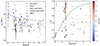 |
Fig. 7. Left: depletion time as a function of redshift for our sample, colour coded as a function of their offset from the MS. The comparison samples are as indicated in Fig. 6, with their mean error shown by the vertical line at z = 0. The solid line shows the expected trend (Tacconi et al. 2018) for a main–sequence galaxy of stellar mass 2 × 10⁹ M⊙, the median of our sample. With depletion timescales in the range 45−900 Myr, most of our sample falls below the locus for normal, star–forming galaxies, and will quickly deplete the gas and transition into quiescence in the absence of gas replenishment. Right: gas fraction (Mgas/(Mgas + M*)) as a function of redshift. The high–redshift unobscured QSOs are not plotted as they lack estimates of their stellar masses. For the QSO comparison samples, the gas mass estimates have been adjusted for αCO = 4. On average, the detected QSOs are very gas–rich, while the non–detected QSOs, which are likely transitioning into quiescence, have almost depleted the available molecular gas. The largest gas fractions are found in the QSOs with the largest offset from the main–sequence, suggesting that the large gas mass is sustaining the high SFRs. |
Figure 7 (right) shows the gas fraction as a function of redshift. The derived stellar masses (Table 4) suggest a wide range of fgas from < 0.02 to 0.97 for our targets, assuming αCO = 4 (< 0.05 − 0.90 if we assumed αCO = 1). The QSOs with the largest offset from the main sequence have the largest gas fractions, suggesting that a larger availability of molecular gas might be fueling the starbursts. The mean fgas = 0.67 ± 0.22 is comparable to what has been found in other high-z QSOs (e.g. Banerji et al. 2017; Venemans et al. 2017; Bischetti et al. 2021), but larger than the gas fractions of SMGs (mean fgas ∼ 0.4, Frias Castillo et al. 2023). There are still large uncertainties in these values due to the large errors of the stellar masses and the uncertain αCO. Using the stellar masses derived from MBH following Ding et al. (2020; see Sect. 3.4) yields equally large gas fractions (0.46−0.98), with a median fgas = 0.77, for the QSOs where molecular gas is detected. Obscured QSOs also show a comparable spread in their gas fractions to those of our sample (Perna et al. 2018 found obscured QSOs to have lower fgas than main–sequence galaxies, although this was driven by their assumption of αCO = 0.8). If we used αCO = 0.8 instead, our QSOs would have a mean fgas = 0.4 ± 0.2, in line with the average gas fraction found for SMGs at high–redshift. This highlights the large uncertainty regarding αCO for QSO–host galaxies, and the crucial need for high–resolution follow–up of the molecular gas in larger samples of QSOs to put stronger constraints on its value via, for example, dynamical modelling (Kakkad et al. 2017; Paraficz et al. 2018).
In Fig. 8 we show how the gas depletion times and gas fractions vary with offset from the main sequence for our sample of unobscured QSOs and the comparison samples from the literature. Our CO detected QSOs follow the decreasing trend seen in the tdep–ΔMS plane. The non–detected QSOs, however, show depletion times about an order of magnitude lower than other SFGs and low–redshift QSOs at similar ΔMS. This further indicates that these QSOs are transitioning into quiescence, and do not follow the relation derived for other star–forming galaxies. The gas fractions clearly increase with ΔMS and follow within the error bars the trend shown by the literature samples. It is important to consider possible systematic uncertainties introduced by our choice of αCO. Although we have tried to control for this by making consistent assumptions for all the QSO and SFG populations, we cannot rule out some level of systematic differences in αCO for our QSOs and those at high redshift, which may be significantly lower due to the starburst nature of some sources. The difference in the conversion factor could systematically shift our sample of QSOs to lower gas fractions and depletion times, increasing the difference with SFGs and SMGs.
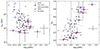 |
Fig. 8. Depletion time (left) and gas fraction (right) as a function of offset from the main sequence (ΔMS) as parameterised by Speagle et al. (2014) for our QSOs (magenta circles). The comparison samples are as indicated in Fig. 6, and we show their combined median error shown by a cross in each panel. For the QSO comparison samples, the gas mass estimates have been adjusted for αCO = 4. The vertical dashed line shows the position for sources on the main–sequence, Δ = 0. Our CO–detected QSOs follow the overall trend shown by the comparison samples of decreasing (increasing) depletion time (gas fraction) with increasing ΔMS. B1608+656 and B1600+434 are outliers in this plot, as they have lower tdep by about an order of magnitude than other star–forming galaxies and QSOs of similar ΔMS, further supporting the idea that they are transitioning into quiescence. |
4.5. Comparison with simulations
It is interesting to compare the results of our survey with predictions from the simulations. We select three of the current generation of hydrodynamic, cosmological simulations: EAGLE (Crain et al. 2015; Schaye et al. 2015), IllustrisTNG100 (Marinacci et al. 2018; Naiman et al. 2018; Nelson et al. 2018; Pillepich et al. 2018; Springel et al. 2018) and SIMBA (Davé et al. 2019). All three simulations have boxes of similar size, L ∼ 100 cMpc (comoving Mpc). Following Ward et al. (2022), we select galaxies at z = 1 with Lbol in the range 1042 − 46 erg s−1 and stellar masses in the range 109 − 12 M⊙ in order to match the properties of our QSOs. We note that previous studies have shown that the SFRs in EAGLE are 0.2 dex lower than observations (Furlong et al. 2015; McAlpine et al. 2017). Additionally, due to the limited volume of the simulations, EAGLE does not reach Lbol = 1046 erg s−1, while IllustrisTNG and SIMBA have very few galaxies in this range. This only affects comparison with J1633+3134, J1650+4251 and B1152+434, which have the highest Lbol.
In Fig. 9 we show the SFR–Mgas plane, where we compare our QSOs with galaxies from the three simulations at z = 1, separated in bins of stellar mass. Despite the boost in signal provided by gravitational lensing, we are only able to probe the upper end of the molecular gas mass distribution with our QSOs. This suggests that it will be challenging to detect non–lensed systems of comparable mass with our current facilities.
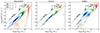 |
Fig. 9. Distribution in the SFR–Mgas plane of the QSOs in this study, colour coded by their stellar mass. The contours show the position of galaxies with Lbol = 1042 − 46 erg s−1 and M* = 109 − 12 M⊙ from the IllustrisTNG (left), EAGLE (middle) and SIMBA (right) hydrodynamical simulations, separated in bins of stellar mass (109 − 10 M⊙, blue; 1010 − 11 M⊙, green; 1011 − 12 M⊙, red). The dashed lines indicate depletion times of 100 Myr and 1 Gyr. Since the SFRs in EAGLE are known to be 0.2 dex lower than observations of main–sequence galaxies (Furlong et al. 2015; McAlpine et al. 2017), we show by how much the SFRs would shift upwards if they matched the observations with the black arrow. The simulations struggle to reproduce the high SFRs of our sample given their low stellar mass, which is likely due to a lack of sufficient resolution in the subgrid physics models. Despite using gravitational lensing to probe fainter systems, we are only probing the upper end of the predicted molecular gas mass distribution, suggesting that it will be challenging to detect non-lensed objects of similar gas masses. |
Looking at the locus of our QSOs in the SFR–Mgas plane, we find that most of their SFRs are underestimated in every simulation, leading to an overestimation of their depletion timescales. This mismatch in SFR values would only worsen if we assumed a lower αCO, which would decrease both the molecular gas mass and the depletion times. Although the simulations do have galaxies with SFRs comparable to those of the QSOs, those values are only expected for galaxies of stellar mass M* ∼ 1011 M⊙. One possible explanation is that AGNFITTER did not properly remove all of the AGN contribution to LIR. However, we do not expect this to decrease the IR luminosities by more than 0.1 dex (Kirkpatrick et al. 2019), which would still not be enough to solve the discrepancy. This tension in SFRs is more likely the result of the difficulty that simulations still have in producing galaxies with elevated SFRs. The lack of starburst galaxies in current hydrodynamical simulations (EAGLE, SIMBA, Illustris, Horizon-AGN) has been pointed out in previous studies of galaxy formation models (e.g. Sparre et al. 2015; Katsianis et al. 2017; Rinaldi et al. 2022). This may be due to the insufficient resolution of galaxy models, which cannot properly model the multiphase ISM, in particular the cold phase where star formation takes place. Star formation in simulations follows the Kennicutt–Schmidt law (Kennicutt 1998). However, in order to produce a starburst, very high densities only reached in the cold phase of the ISM are necessary. But if the molecular gas gets too cold and dense, the Jeans mass and length become smaller than the resolved mass of the simulation. Therefore, to prevent this from happening, a pressure floor is imposed on the simulation, thereby preventing the gas from becoming cold and dense enough to produce a starburst.
5. Discussion
In the canonical picture of massive galaxy evolution (Sanders & Mirabel 1985; Alexander et al. 2005; Hopkins et al. 2008), unobscured QSO hosts are the end product of the merger between two gas–rich galaxies, and are expected to be systematically gas–poorer than “normal” galaxies with the same stellar mass and have little remaining star formation due to QSO feedback. Many studies have explored the gas content in QSO hosts compared to non–QSO systems, both at low (e.g. Rosario et al. 2018; Jarvis et al. 2020; Shangguan et al. 2020b; Ramos Almeida et al. 2022) and high redshift (e.g. Kakkad et al. 2017; Perna et al. 2018; D’Amato et al. 2020; Kirkpatrick et al. 2019; Bischetti et al. 2021). While these studies are very heterogeneous, there is a growing consensus that QSO host galaxies are as gas–rich as their non–QSO counterparts, a conclusion supported by state–of–the-art simulations (Ward et al. 2022). This however depends on the highly uncertain αCO value for QSOs, to which the gas fraction is very sensitive.
We have detected CO(2–1) line emission in 70% of our sample of FIR–bright, unobscured QSOs (Fig. 1). The derived gas masses of < 1.6−36 (αCO/4) × 109 M⊙ are about an order of magnitude below those of normal, star–forming galaxies (Fig. 6). Our SED analysis reveals that these systems also have lower stellar masses than the average population of obscured and unobscured high–redshift QSOs, which we are able to detect thanks to gravitational lensing. These are therefore likely to be a younger and/or less massive population than the high–redshift QSOs studied so far. Nevertheless, we infer gas fractions between < 2% and 97% (for αCO = 4, Fig. 7), although with large errors introduced by uncertainties in the stellar mass. Taken at face value, our sample thus spans the entire physical range of fgas, including both very gas–rich and gas–poor galaxies. However, five of our targets are conspicuously gas–rich, with fgas > 50%. These gas fractions are comparable to –or exceeding– typical main sequence galaxies at their redshift and stellar mass (for example, ASPECS MS galaxies in Figs. 4 and 7), and support the results from previous studies pointing towards QSO–host being as gas–rich as non–QSO hosts (e.g. Kakkad et al. 2017; Rodighiero et al. 2019; D’Amato et al. 2020; Jarvis et al. 2020; Shangguan et al. 2020b). Recent cosmological simulations also predict that luminous AGN are associated with gas–rich star–forming galaxies (Ward et al. 2022). This co–existence of star formation and AGN activity (Floyd et al. 2013; Stanley et al. 2017; Symeonidis et al. 2022) is likely caused by the supply of cold molecular gas driving both phenomena. Nevertheless, high gas fractions do not mean that AGN feedback is not affecting the gas reservoirs of the galaxies, but, considering the short timescales of QSO activity, it becomes challenging to detect their impact on ffgas. Instead, it is likely that the cumulative effects of several episodes of AGN activity are necessary to significantly depress the gas fractions (Piotrowska et al. 2022), and could indicate that the central AGN in B1608+656, B1152+200 and B1600+434 have been active for a longer period of time compared to the rest of the sample.
Despite the large gas fractions, the high star formation rates of our targets imply that the available molecular gas will quickly be depleted, and star formation will subsequently quench. The depletion times of ∼90 Myr (or ∼25 Myr for αCO = 1, Fig. 7) suggest that these galaxies will quench and turn into gas–poor unobscured QSOs during the lifetime of the quasar, rather than much shorter timescales of ∼1 Myr, as had been suggested by Simpson et al. (2012). Such short depletion times have been routinely found in other high–redshift QSOs (e.g. Paraficz et al. 2018, although see Riechers 2011; Bischetti et al. 2021), and are significantly below those of low–redshift QSOs, with tdep ∼ 1 Gyr.
In summary, the current data for our sample of QSOs suggests that the high star formation rates are enough to explain the deficit in CO luminosity (Fig. 5) and short depletion times (Figs. 7 and 8). While this does not rule out the presence of feedback, current or past, from the central AGN which might be falling bellow the detection limit of our NOEMA observations, the high gas fractions and lack of evidence for cold gas outflows suggest however that, if present, AGN feedback has not significantly impacted the gas reservoirs yet. Nevertheless, outflows observed in luminous QSOs typically correspond to ∼2% of the peak of the CO emission line profiles (e.g. Feruglio et al. 2017), so deeper CO(2–1) observations would be required to determine the prevalence of ongoing outflows in these targets. Along with higher angular resolution observations of low J-level CO and FIR emission to probe the size and distribution of the cold gas and dust reservoirs, these diagnostics will be useful to determine the relative importance of AGN and stellar feedback in the process of quenching in QSO–host galaxies. Higher angular resolution observations would also help study the impact of galaxy morphology the molecular gas content of our sample of QSOs, as Husemann et al. (2017) and Ramos Almeida et al. (2022) found that disc–dominated and merging QSOs have larger gas masses than bulge–dominated QSOs.
Finally, B1608+656, B1152+200 and B1600+434 have not been detected in CO emission. These are three of the four radio–loud QSOs in our sample, and show bright continuum (λrest = 1.3 mm) emission likely arising from the central AGN and have molecular gas masses Mgas < 109 M⊙. These radio jets are likely to cause jet–mode AGN feedback that will impact the gas–reservoirs of these radio–loud, QSO–host galaxies, possibly over a long period of time (e.g. Mukherjee et al. 2018; Fotopoulou et al. 2019; Jarvis et al. 2019; Zovaro et al. 2019; Couto & Storchi-Bergmann 2023; Tamhane et al. 2023). MG 0414+0534 is another radio–loud, unobscured QSO detected in mid–J CO emission (Barvainis et al. 1998) but not in low–J emission (Sharon et al. 2016). Conversely, radio–loud but obscured QSOs such as B1938+666 (Sharon et al. 2016) or MG 0751+2716 (Riechers 2011) do show low–excitation gas reservoirs detected in CO(1–0). If obscured and unobscured radio–loud QSOs are evolutionary connected, this would be consistent with the radio–loud, obscured phase occurring earlier, until eventually the heat and turbulence injected by the radio jets reduce the cold molecular gas and star formation halts. A larger, well–defined sample of both obscured and unobscured, radio–loud QSOs observed in low–J emission will be needed to explore this scenario.
6. Conclusions
We have presented NOEMA observations of CO(2–1) line and continuum emission in a sample of ten gravitationally lensed, unobscured QSOs at z = 1 − 1.5. These observations significantly increase the number of unobscured QSOs detected in CO line emission in this redshift range. Our main conclusions are as follows:
– We detect CO(2–1) in seven of our targets (70% detection rate), with line luminosities of 0.9−7.7 × 10⁹ K km s−1 pc2. For the three QSOs not detected, we place 3σ upper limits on their line luminosities of ≤0.4 × 10⁹ K km s−1 pc2. We also detect far–infrared continuum emission underlying the CO line emission in four of the CO–detected targets. Three out of the four radio–loud QSOs in our sample show no CO emission but have very strong (S/N > 200) continuum emission, likely originating from the radio jets. Although we currently do not find evidence of outflows in any of the targets detected in CO(2–1), more data is needed to definitively rule out significant on-going outflow activity contributing to further gas depletion in the QSOs.
– We collect the available photometry for the ten targets and separate the emission coming from the lens and lensed galaxies. We then fit the SED of the lensed QSOs and their host galaxies using AGNFITTER. We find a large range of stellar masses and SFRs which, according to empirical scaling relations, classify six of the targets as starbursts (ΔMS > 0.6 dex), with three more consistent with being on the main sequence of star–forming galaxies. Our study supports the idea that AGN and starburst activity co–exist in the host galaxies of FIR–bright, unobscured QSO. If there is any significant SFR suppression by AGN feedback, it must occur on longer timescales. The three radio–loud QSOs not detected in CO, however, fall on or below the main–sequence, which suggests that they are transitioning into quiescence.
– Only three of our targets fall within the scatter of the  empirical relation for either star–forming or starburst galaxies. The seven remaining QSOs fall well below this relation. This could be a sign of AGN or star formation feedback either depleting the molecular gas reservoir or heating up the gas and thus preventing it from collapsing to form new stars. We find the largest outliers from the
  relation to be the three non–detected QSOs. Along with their position on the main–sequence, short gas depletion times and low gas fractions, we interpret this as a possible sign of jet–mode AGN feedback contributing to the depletion of the gas reservoirs in these sources.
– We find total cold molecular gas masses in the range ≤2−30 × 109 (αCO/4) M⊙. This implies high gas fractions of ∼50% (for αCO = 4) for the detected galaxies. Despite these targets being gas–rich, the high SFRs result in a range of depletion times of 50−900 Myr, with a median of only ∼90 Myr, a factor of 7 below the expected value for main–sequence galaxies. These short depletion times are only reinforced if we assume a starburst–like conversion factor of αCO = 1. Our QSOs are thus undergoing a period of intense growth, and will quickly turn the available gas into stars, subsequently quenching star formation.
– We compare our QSOs with galaxies from the hydrodynamical simulations IllustrisTNG100, EAGLE, and SIMBA, in the same redshift, stellar mass and bolometric luminosity intervals. We show that, while our sample is comparable in total gas mass to the most gas–rich galaxies selected, the simulations struggle to reproduce their high SFRs and thus overestimate their gas depletion times, especially when we compare in smaller bins of stellar mass. This lack of starbursts is linked to the fact that the current simulations do not have the necessary resolution to successfully model the small scale physics involved in the starburst phenomenon, as has been previously noted for the bulk of the simulated galaxy population.
The NOEMA observations analysed in this work provide important information about the properties of the cold ISM of FIR–bright, unobscured QSOs just after the peak epoch of QSO activity and massive galaxy assembly. We find that these systems lie preferentially in low–mass, gas–rich host galaxies undergoing starbursts. This phase of intense growth will use up the molecular gas reservoir in a few hundreds of Myr. Follow-up observations with higher angular resolution are needed to map the cold gas kinematics in their hosts and establish the presence of merger signatures to better understand the cause of the intense starburst, as well as to establish the importance of AGN feedback in the depletion of the gas reservoirs.
Independent AGNFITTER models for the spectral energy distributions of J0924+0219 and J1330+1810 were recently presented by Stacey et al. (2022). Compared to the Stacey et al. models which assumed that the optical emission is dominated by the QSO component, we removed the foreground contamination and used wider priors which allow optical emissions to be dominated by the stellar component. On average, our approach yielded slightly lower QSO luminosities in the optical.
For all QSOs except B1608+656 and B1600+434, which were not in the catalogue in Rakshit et al. (2020).
Acknowledgments
We would like to thank the anonymous referee for their constructive comments that helped significantly improve this work. This work is based on observations carried out under projects S19CC and W20CM with the IRAM NOEMA Interferometer. IRAM is supported by INSU/CNRS (France), MPG (Germany) and IGN (Spain). M.F.C. and M.R. thank IRAM and J.M. Winters in particular for hosting the online data reduction. M.R. is supported by the NWO Veni project “Under the lens” (VI.Veni.202.225). M.F.C., M.R. and J.H. acknowledge support of the VIDI research programme with project number 639.042.611, which is (partly) financed by the Netherlands Organisation for Scientific Research (NWO). J.H. acknowledges support from the ERC Consolidator Grant 101088676 (VOYAJ). C.M.H. acknowledges funding from an United Kingdom Research and Innovation grant (code: MR/V022830/1). S.R.W. acknowledges funding from the Deutsche Forschungsgemeinschaft (DFG, German Research Foundation) under Germany’s Excellence Strategy: EXC2094-390783311. This work is based on the research supported in part by the National Research Foundation of South Africa (Grant Numbers: 128943). The NASA/IPAC Extragalactic Database (NED) is funded by the National Aeronautics and Space Administration and operated by the California Institute of Technology. The research leading to these results has received funding from the European Union’s Horizon 2020 research and innovation program under grant agreement No. 730562 [RadioNet].
References
- Accurso, G., Saintonge, A., Catinella, B., et al. 2017, MNRAS, 470, 4750 [NASA ADS] [Google Scholar]
- Alexander, D. M., Smail, I., Bauer, F. E., et al. 2005, Nature, 434, 738 [NASA ADS] [CrossRef] [Google Scholar]
- Banerji, M., Carilli, C. L., Jones, G., et al. 2017, MNRAS, 465, 4390 [Google Scholar]
- Barvainis, R., & Ivison, R. 2002, ApJ, 571, 712 [Google Scholar]
- Barvainis, R., Alloin, D., Guilloteau, S., & Antonucci, R. 1998, ApJ, 492, L13 [Google Scholar]
- Barvainis, R., Alloin, D., & Bremer, M. 2002, A&A, 385, 399 [NASA ADS] [CrossRef] [EDP Sciences] [Google Scholar]
- Bigiel, F., Leroy, A., Walter, F., et al. 2008, AJ, 136, 2846 [NASA ADS] [CrossRef] [Google Scholar]
- Birkin, J. E., Weiss, A., Wardlow, J. L., et al. 2021, MNRAS, 501, 3926 [Google Scholar]
- Bischetti, M., Maiolino, R., Carniani, S., et al. 2019, A&A, 630, A59 [NASA ADS] [CrossRef] [EDP Sciences] [Google Scholar]
- Bischetti, M., Feruglio, C., Piconcelli, E., et al. 2021, A&A, 645, A33 [NASA ADS] [CrossRef] [EDP Sciences] [Google Scholar]
- Bolatto, A. D., Wolfire, M., & Leroy, A. K. 2013, ARA&A, 51, 207 [CrossRef] [Google Scholar]
- Boogaard, L. A., van der Werf, P., Weiss, A., et al. 2020, ApJ, 902, 109 [NASA ADS] [CrossRef] [Google Scholar]
- Brown, M. J. I., Moustakas, J., Smith, J. D. T., et al. 2014, ApJS, 212, 18 [Google Scholar]
- Browne, I. W. A., Wilkinson, P. N., Jackson, N. J. F., et al. 2003, MNRAS, 341, 13 [NASA ADS] [CrossRef] [Google Scholar]
- Brusa, M., Cresci, G., Daddi, E., et al. 2018, A&A, 612, A29 [NASA ADS] [CrossRef] [EDP Sciences] [Google Scholar]
- Butler, K. M., van der Werf, P. P., Omont, A., & Cox, P. 2023, A&A, 674, L5 [NASA ADS] [CrossRef] [EDP Sciences] [Google Scholar]
- Calistro Rivera, G., Lusso, E., Hennawi, J. F., & Hogg, D. W. 2016, ApJ, 833, 98 [Google Scholar]
- Calistro Rivera, G., Alexander, D. M., Rosario, D. J., et al. 2021, A&A, 649, A102 [NASA ADS] [CrossRef] [EDP Sciences] [Google Scholar]
- Carilli, C. L., & Walter, F. 2013, ARA&A, 51, 105 [NASA ADS] [CrossRef] [Google Scholar]
- Carraro, R., Rodighiero, G., Cassata, P., et al. 2020, A&A, 642, A65 [EDP Sciences] [Google Scholar]
- Casey, C. M., Narayanan, D., & Cooray, A. 2014, Phys. Rep., 541, 45 [Google Scholar]
- Chabrier, G. 2003, PASP, 115, 763 [Google Scholar]
- Chartas, G., Davidson, E., Brusa, M., et al. 2020, MNRAS, 496, 598 [Google Scholar]
- Cicone, C., Maiolino, R., Sturm, E., et al. 2014, A&A, 562, A21 [NASA ADS] [CrossRef] [EDP Sciences] [Google Scholar]
- Circosta, C., Mainieri, V., Lamperti, I., et al. 2021, A&A, 646, A96 [EDP Sciences] [Google Scholar]
- Combes, F. 2018, A&ARv, 26, 5 [NASA ADS] [CrossRef] [Google Scholar]
- Couto, G. S., & Storchi-Bergmann, T. 2023, Galaxies, 11, 47 [NASA ADS] [CrossRef] [Google Scholar]
- Cowie, L. L., Songaila, A., Hu, E. M., & Cohen, J. G. 1996, AJ, 112, 839 [Google Scholar]
- Crain, R. A., Schaye, J., Bower, R. G., et al. 2015, MNRAS, 450, 1937 [NASA ADS] [CrossRef] [Google Scholar]
- da Cunha, E., Charlot, S., & Elbaz, D. 2008, MNRAS, 388, 1595 [Google Scholar]
- da Cunha, E., Walter, F., Smail, I. R., et al. 2015, ApJ, 806, 110 [Google Scholar]
- D’Amato, Q., Gilli, R., Vignali, C., et al. 2020, A&A, 636, A37 [NASA ADS] [CrossRef] [EDP Sciences] [Google Scholar]
- Davé, R., Anglés-Alcázar, D., Narayanan, D., et al. 2019, MNRAS, 486, 2827 [Google Scholar]
- Del Moro, A., Alexander, D. M., Mullaney, J. R., et al. 2013, A&A, 549, A59 [NASA ADS] [CrossRef] [EDP Sciences] [Google Scholar]
- Delvecchio, I., Gruppioni, C., Pozzi, F., et al. 2014, MNRAS, 439, 2736 [NASA ADS] [CrossRef] [Google Scholar]
- Di Matteo, P., Combes, F., Melchior, A. L., & Semelin, B. 2007, A&A, 468, 61 [NASA ADS] [CrossRef] [EDP Sciences] [Google Scholar]
- Ding, X., Silverman, J., Treu, T., et al. 2020, ApJ, 888, 37 [NASA ADS] [CrossRef] [Google Scholar]
- Dunne, L., Maddox, S. J., Papadopoulos, P. P., Ivison, R. J., & Gomez, H. L. 2022, MNRAS, 517, 962 [NASA ADS] [CrossRef] [Google Scholar]
- Elbaz, D., Dickinson, M., Hwang, H. S., et al. 2011, A&A, 533, A119 [NASA ADS] [CrossRef] [EDP Sciences] [Google Scholar]
- Ferrarese, L., & Merritt, D. 2000, ApJ, 539, L9 [Google Scholar]
- Feruglio, C., Ferrara, A., Bischetti, M., et al. 2017, A&A, 608, A30 [NASA ADS] [CrossRef] [EDP Sciences] [Google Scholar]
- Feruglio, C., Fiore, F., Carniani, S., et al. 2018, A&A, 619, A39 [NASA ADS] [CrossRef] [EDP Sciences] [Google Scholar]
- Floyd, D. J. E., Dunlop, J. S., Kukula, M. J., et al. 2013, MNRAS, 429, 2 [NASA ADS] [CrossRef] [Google Scholar]
- Fontanot, F., De Lucia, G., Monaco, P., Somerville, R. S., & Santini, P. 2009, MNRAS, 397, 1776 [NASA ADS] [CrossRef] [Google Scholar]
- Fotopoulou, C. M., Dasyra, K. M., Combes, F., Salomé, P., & Papachristou, M. 2019, A&A, 629, A30 [NASA ADS] [CrossRef] [EDP Sciences] [Google Scholar]
- Frias Castillo, M., Hodge, J., Rybak, M., et al. 2023, ApJ, 945, 128 [NASA ADS] [CrossRef] [Google Scholar]
- Furlong, M., Bower, R. G., Theuns, T., et al. 2015, MNRAS, 450, 4486 [Google Scholar]
- Gebhardt, K., Bender, R., Bower, G., et al. 2000, ApJ, 539, L13 [Google Scholar]
- Genzel, R., Tacconi, L. J., Gracia-Carpio, J., et al. 2010, MNRAS, 407, 2091 [NASA ADS] [CrossRef] [Google Scholar]
- Griffin, M. J., Abergel, A., Abreu, A., et al. 2010, A&A, 518, L3 [EDP Sciences] [Google Scholar]
- Gürkan, G., Hardcastle, M. J., Jarvis, M. J., et al. 2015, MNRAS, 452, 3776 [CrossRef] [Google Scholar]
- Harris, K., Farrah, D., Schulz, B., et al. 2016, MNRAS, 457, 4179 [NASA ADS] [CrossRef] [Google Scholar]
- Hopkins, P. F., Somerville, R. S., Hernquist, L., et al. 2006, ApJ, 652, 864 [NASA ADS] [CrossRef] [Google Scholar]
- Hopkins, P. F., Hernquist, L., Cox, T. J., & Kereš, D. 2008, ApJS, 175, 356 [Google Scholar]
- Husemann, B., Davis, T. A., Jahnke, K., et al. 2017, MNRAS, 470, 1570 [NASA ADS] [CrossRef] [Google Scholar]
- Izumi, T., Nguyen, D. D., Imanishi, M., et al. 2020, ApJ, 898, 75 [NASA ADS] [CrossRef] [Google Scholar]
- Jarvis, M. E., Harrison, C. M., Thomson, A. P., et al. 2019, MNRAS, 485, 2710 [Google Scholar]
- Jarvis, M. E., Harrison, C. M., Mainieri, V., et al. 2020, MNRAS, 498, 1560 [NASA ADS] [CrossRef] [Google Scholar]
- Kakkad, D., Mainieri, V., Brusa, M., et al. 2017, MNRAS, 468, 4205 [Google Scholar]
- Katsianis, A., Blanc, G., Lagos, C. P., et al. 2017, MNRAS, 472, 919 [NASA ADS] [CrossRef] [Google Scholar]
- Kayo, I., Inada, N., Oguri, M., et al. 2010, AJ, 139, 1614 [NASA ADS] [CrossRef] [Google Scholar]
- Kennicutt, R. C., Jr. 1998, ApJ, 498, 541 [Google Scholar]
- Kirkpatrick, A., Sharon, C., Keller, E., & Pope, A. 2019, ApJ, 879, 41 [NASA ADS] [CrossRef] [Google Scholar]
- Kormendy, J., & Ho, L. C. 2013, ARA&A, 51, 511 [Google Scholar]
- Koss, M. J., Strittmatter, B., Lamperti, I., et al. 2021, ApJS, 252, 29 [CrossRef] [Google Scholar]
- Krips, M., Neri, R., Eckart, A., et al. 2005, A&A, 431, 879 [NASA ADS] [CrossRef] [EDP Sciences] [Google Scholar]
- Leslie, S. K., Schinnerer, E., Liu, D., et al. 2020, ApJ, 899, 58 [Google Scholar]
- Li, F., Wang, J., Fang, M., et al. 2020, PASJ, 72, 41 [NASA ADS] [CrossRef] [Google Scholar]
- Lutz, D., Sturm, E., Janssen, A., et al. 2020, A&A, 633, A134 [NASA ADS] [CrossRef] [EDP Sciences] [Google Scholar]
- Madau, P., & Dickinson, M. 2014, ARA&A, 52, 415 [Google Scholar]
- Maiolino, R., Gallerani, S., Neri, R., et al. 2012, MNRAS, 425, L66 [Google Scholar]
- Maloney, P. R., Hollenbach, D. J., & Tielens, A. G. G. M. 1996, ApJ, 466, 561 [Google Scholar]
- Marinacci, F., Vogelsberger, M., Pakmor, R., et al. 2018, MNRAS, 480, 5113 [NASA ADS] [Google Scholar]
- McAlpine, S., Bower, R. G., Harrison, C. M., et al. 2017, MNRAS, 468, 3395 [NASA ADS] [CrossRef] [Google Scholar]
- McMullin, J. P., Waters, B., Schiebel, D., Young, W., & Golap, K. 2007, ASP Conf. Ser., 376, 127 [Google Scholar]
- Mortlock, A., Conselice, C. J., Bluck, A. F. L., et al. 2011, MNRAS, 413, 2845 [Google Scholar]
- Mukherjee, D., Wagner, A. Y., Bicknell, G. V., et al. 2018, MNRAS, 476, 80 [NASA ADS] [CrossRef] [Google Scholar]
- Mullaney, J. R., Alexander, D. M., Goulding, A. D., & Hickox, R. C. 2011, MNRAS, 414, 1082 [Google Scholar]
- Murphy, E. J., Condon, J. J., Schinnerer, E., et al. 2011, ApJ, 737, 67 [Google Scholar]
- Naiman, J. P., Pillepich, A., Springel, V., et al. 2018, MNRAS, 477, 1206 [Google Scholar]
- Nelson, D., Pillepich, A., Springel, V., et al. 2018, MNRAS, 475, 624 [Google Scholar]
- Netzer, H., Lani, C., Nordon, R., et al. 2016, ApJ, 819, 123 [Google Scholar]
- Noeske, K. G., Weiner, B. J., Faber, S. M., et al. 2007, ApJ, 660, L43 [CrossRef] [Google Scholar]
- Oguri, M., Inada, N., Clocchiatti, A., et al. 2008, AJ, 135, 520 [NASA ADS] [CrossRef] [Google Scholar]
- Page, M. J., Symeonidis, M., Vieira, J. D., et al. 2012, Nature, 485, 213 [NASA ADS] [CrossRef] [Google Scholar]
- Paraficz, D., Rybak, M., McKean, J. P., et al. 2018, A&A, 613, A34 [NASA ADS] [CrossRef] [EDP Sciences] [Google Scholar]
- Perna, M., Sargent, M. T., Brusa, M., et al. 2018, A&A, 619, A90 [NASA ADS] [CrossRef] [EDP Sciences] [Google Scholar]
- Pilbratt, G. L., Riedinger, J. R., Passvogel, T., et al. 2010, A&A, 518, L1 [NASA ADS] [CrossRef] [EDP Sciences] [Google Scholar]
- Pillepich, A., Springel, V., Nelson, D., et al. 2018, MNRAS, 473, 4077 [Google Scholar]
- Piotrowska, J. M., Bluck, A. F. L., Maiolino, R., & Peng, Y. 2022, MNRAS, 512, 1052 [NASA ADS] [CrossRef] [Google Scholar]
- Pitchford, L. K., Hatziminaoglou, E., Feltre, A., et al. 2016, MNRAS, 462, 4067 [NASA ADS] [CrossRef] [Google Scholar]
- Planck Collaboration XIII. 2016, A&A, 594, A13 [NASA ADS] [CrossRef] [EDP Sciences] [Google Scholar]
- Rakshit, S., Stalin, C. S., & Kotilainen, J. 2020, ApJS, 249, 17 [Google Scholar]
- Ramos Almeida, C., Bischetti, M., García-Burillo, S., et al. 2022, A&A, 658, A155 [NASA ADS] [CrossRef] [EDP Sciences] [Google Scholar]
- Riechers, D. A. 2011, ApJ, 730, 108 [NASA ADS] [CrossRef] [Google Scholar]
- Rinaldi, P., Caputi, K. I., van Mierlo, S. E., et al. 2022, ApJ, 930, 128 [NASA ADS] [CrossRef] [Google Scholar]
- Rodighiero, G., Daddi, E., Baronchelli, I., et al. 2011, ApJ, 739, L40 [Google Scholar]
- Rodighiero, G., Enia, A., Delvecchio, I., et al. 2019, ApJ, 877, L38 [NASA ADS] [CrossRef] [Google Scholar]
- Rosario, D. J., Trakhtenbrot, B., Lutz, D., et al. 2013, A&A, 560, A72 [NASA ADS] [CrossRef] [EDP Sciences] [Google Scholar]
- Rosario, D. J., Burtscher, L., Davies, R. I., et al. 2018, MNRAS, 473, 5658 [NASA ADS] [CrossRef] [Google Scholar]
- Rybak, M., Hodge, J. A., Vegetti, S., et al. 2020, MNRAS, 494, 5542 [NASA ADS] [CrossRef] [Google Scholar]
- Rybak, M., Hodge, J. A., Greve, T. R., et al. 2022, A&A, 667, A70 [NASA ADS] [CrossRef] [EDP Sciences] [Google Scholar]
- Saintonge, A., Kauffmann, G., Wang, J., et al. 2011, MNRAS, 415, 61 [NASA ADS] [CrossRef] [Google Scholar]
- Sanders, D. B., & Mirabel, I. F. 1985, ApJ, 298, L31 [Google Scholar]
- Sanders, D. B., Soifer, B. T., Elias, J. H., et al. 1988, ApJ, 325, 74 [Google Scholar]
- Sargent, M. T., Daddi, E., Béthermin, M., et al. 2014, ApJ, 793, 19 [NASA ADS] [CrossRef] [Google Scholar]
- Schaye, J., Crain, R. A., Bower, R. G., et al. 2015, MNRAS, 446, 521 [Google Scholar]
- Schreiber, C., Pannella, M., Elbaz, D., et al. 2015, A&A, 575, A74 [NASA ADS] [CrossRef] [EDP Sciences] [Google Scholar]
- Shangguan, J., Ho, L. C., Bauer, F. E., Wang, R., & Treister, E. 2020a, ApJ, 899, 112 [NASA ADS] [CrossRef] [Google Scholar]
- Shangguan, J., Ho, L. C., Bauer, F. E., Wang, R., & Treister, E. 2020b, ApJS, 247, 15 [NASA ADS] [CrossRef] [Google Scholar]
- Shankar, F., Weinberg, D. H., & Miralda-Escudé, J. 2009, ApJ, 690, 20 [NASA ADS] [CrossRef] [Google Scholar]
- Sharon, C. E., Riechers, D. A., Hodge, J., et al. 2016, ApJ, 827, 18 [Google Scholar]
- Simpson, J. M., Smail, I., Swinbank, A. M., et al. 2012, MNRAS, 426, 3201 [Google Scholar]
- Solomon, P. M., & Vanden Bout, P. A. 2005, ARA&A, 43, 677 [NASA ADS] [CrossRef] [Google Scholar]
- Somerville, R. S., & Davé, R. 2015, ARA&A, 53, 51 [Google Scholar]
- Somerville, R. S., Hopkins, P. F., Cox, T. J., Robertson, B. E., & Hernquist, L. 2008, MNRAS, 391, 481 [NASA ADS] [CrossRef] [Google Scholar]
- Sparre, M., Hayward, C. C., Springel, V., et al. 2015, MNRAS, 447, 3548 [Google Scholar]
- Speagle, J. S., Steinhardt, C. L., Capak, P. L., & Silverman, J. D. 2014, ApJS, 214, 15 [Google Scholar]
- Spilker, J. S., Aravena, M., Phadke, K. A., et al. 2020, ApJ, 905, 86 [Google Scholar]
- Spingola, C., McKean, J. P., Vegetti, S., et al. 2020, MNRAS, 495, 2387 [Google Scholar]
- Springel, V., Pakmor, R., Pillepich, A., et al. 2018, MNRAS, 475, 676 [Google Scholar]
- Stacey, H. R., McKean, J. P., Robertson, N. C., et al. 2018, MNRAS, 476, 5075 [NASA ADS] [CrossRef] [Google Scholar]
- Stacey, H. R., McKean, J. P., Powell, D. M., et al. 2021, MNRAS, 500, 3667 [Google Scholar]
- Stacey, H. R., Costa, T., McKean, J. P., et al. 2022, MNRAS, 517, 3377 [NASA ADS] [CrossRef] [Google Scholar]
- Stanley, F., Alexander, D. M., Harrison, C. M., et al. 2017, MNRAS, 472, 2221 [Google Scholar]
- Storchi-Bergmann, T., & Schnorr-Müller, A. 2019, Nat. Astron., 3, 48 [Google Scholar]
- Symeonidis, M., Maddox, N., Jarvis, M. J., et al. 2022, MNRAS, 514, 4450 [CrossRef] [Google Scholar]
- Tacconi, L. J., Genzel, R., Saintonge, A., et al. 2018, ApJ, 853, 179 [Google Scholar]
- Tamhane, P. D., McNamara, B. R., Russell, H. R., et al. 2023, MNRAS, 519, 3338 [NASA ADS] [CrossRef] [Google Scholar]
- Valentino, F., Daddi, E., Puglisi, A., et al. 2021, A&A, 654, A165 [NASA ADS] [CrossRef] [EDP Sciences] [Google Scholar]
- Venemans, B. P., Walter, F., Decarli, R., et al. 2017, ApJ, 845, 154 [Google Scholar]
- Wang, R., Wu, X.-B., Neri, R., et al. 2016, ApJ, 830, 53 [Google Scholar]
- Ward, S. R., Harrison, C. M., Costa, T., & Mainieri, V. 2022, MNRAS, 514, 2936 [NASA ADS] [CrossRef] [Google Scholar]
- Yesuf, H. M., & Ho, L. C. 2020, ApJ, 900, 107 [NASA ADS] [CrossRef] [Google Scholar]
- Zhuang, M.-Y., Ho, L. C., & Shangguan, J. 2021, ApJ, 906, 38 [NASA ADS] [CrossRef] [Google Scholar]
- Zovaro, H. R. M., Nesvadba, N. P. H., Sharp, R., et al. 2019, MNRAS, 489, 4944 [CrossRef] [Google Scholar]
Appendix A: Observations summary
Summary of NOEMA observations: target ID, date of observations, antenna configuration, total and on-source time (ttot and ton).
Appendix B: SED fits
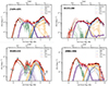 |
Fig. B.1. From top left to bottom right: SED fitting of J1524+4409, B1608+656, J1330+1810, J1455+1447, J1633+3134, and J0924+0214. The black dots represent the observed data points; 3σ upper limits are shown as downward arrows. The best-fit SED obtained with AGNfitter (Calistro Rivera et al. 2016), as well as the different components used to model the total flux are shown as labelled in the figure. Ten realisations picked from the posterior distribution are shown. |
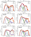 |
Fig. B.2. Fig. B.1 continued. From top left to bottom right: SED fitting of J1650+4251, B1152+200, B1600+434, and J0806+2006. |
All Tables
NOEMA imaging: final synthesised beam sizes and sensitivity for the integrated continuum (given at 1.3 mm rest-frame) and 20 MHz bandwidth at the position of the CO(2–1) line (∼60 km s−1), for natural weighting.
Summary of NOEMA observations: target ID, date of observations, antenna configuration, total and on-source time (ttot and ton).
All Figures
|
Fig. 1. CO(2–1) spectra and 0th moment maps for the detected QSOs. The black solid line indicates the best fit Gaussian model, and the reference velocity was determined based on the redshift derived from the Gaussian fit (LSRK frame). Contours in the 0th moment maps start at 4σ and increase in steps of 4σ for J1524+2209, J1330+1810, J0924+0219, and J1650+4251; contours for J1455+1447, J1633+3134, and J0806+2006 start at 2σ and increase in steps of 2σ. We have used the AIC criterion to determine whether a single- or double–Gaussian fit is more appropriate for the profiles. |
| In the text | |
|
Fig. 1. continued. |
| In the text | |
|
Fig. 2. Detected continuum emission at the position of the CO(2–1) emission line for the sample presented in this work. Contours for J1524+4409, J1330+1810, J1633+3134, and J1650+4251 start at ±2σ and increase in intervals of ±1σ, where σ is given in Table 2. Contours are given in steps of ±50σ starting at 50σ for B1608 and in steps of ±100σ starting at 100σ for B1152 and B1600. The red cross indicates the peak position of the gas emission where detected, and the optical emission for the three QSOs not detected in CO(2–1). |
| In the text | |
|
Fig. 3. Stacked spectrum of our NOEMA observations over the region covering the HCN/HCO+/HNC(3–2) lines. The spectrum was scaled to an apparent FIR luminosity LFIR = 5 × 10¹² L⊙. We did not find any line detected at ≥3σ significance, indicated by the dashed horizontal line. |
| In the text | |
|
Fig. 4. SFR as a function of stellar mass for our sample of unobscured QSOs. The values were obtained through SED fitting with AGNFITTER. For comparison, we have plotted the low–redshift Palomar–Green QSOs from Shangguan et al. (2020b) (grey), high–redshift obscured QSOs (grey, empty circles) from the compilation presented in Perna et al. (2018), a sample of high–redshift SMGs (black stars) and z = 1 − 3 SFGs from ASPECS (blue crosses, Boogaard et al. 2020). The dashed black line marks the main–sequence at z = 1.5 as parameterised by Speagle et al. (2014), with the one sigma scatter shown by the shaded grey area. All data points have been scaled to z = 1.25 for comparison and corrected for magnification where necessary. Most of our targets lie on or above the main–sequence. Their stellar masses are lower than most of the higher–redshift obscured QSOs, but comparable to low–redshift unobscured QSOs and the ASPECS SFGs. |
| In the text | |
|
Fig. 5. Left: CO(1–0) line luminosity versus infrared luminosity integrated over 8−1000 μm for our sample of unobscured QSOs, coloured as a function of offset from the MS. The CO(1–0) luminosities have been calculated using r21 = 0.86 (Kirkpatrick et al. 2019), and LIR has been corrected for AGN contamination. For comparison, we have plotted the low–redshift Palomar–Green QSOs from Shangguan et al. (2020b), high–redshift obscured (filled grey circles) and unobscured (open grey circles) QSOs from the compilation presented in Perna et al. (2018), a sample of high–redshift SMGs (black stars) and z = 1 − 3 SFGs from ASPECS (Boogaard et al. 2020, blue crosses). Where necessary, all quantities have been corrected for magnification. The black solid and dashed lines show the |
| In the text | |
|
Fig. 6. CO(1–0) line luminosities as a function of redshift for our sample. In some cases, error bars are smaller than the marker. The comparison samples are described in Fig. 5. Where necessary, all quantities have been corrected for magnification. On average, the unobscured QSOs targeted in this study have lower CO luminosities than other obscured QSOs and star–forming galaxies at similar redshift. It is thanks to gravitational lensing that we are able to detect these systems with short exposure times. |
| In the text | |
|
Fig. 7. Left: depletion time as a function of redshift for our sample, colour coded as a function of their offset from the MS. The comparison samples are as indicated in Fig. 6, with their mean error shown by the vertical line at z = 0. The solid line shows the expected trend (Tacconi et al. 2018) for a main–sequence galaxy of stellar mass 2 × 10⁹ M⊙, the median of our sample. With depletion timescales in the range 45−900 Myr, most of our sample falls below the locus for normal, star–forming galaxies, and will quickly deplete the gas and transition into quiescence in the absence of gas replenishment. Right: gas fraction (Mgas/(Mgas + M*)) as a function of redshift. The high–redshift unobscured QSOs are not plotted as they lack estimates of their stellar masses. For the QSO comparison samples, the gas mass estimates have been adjusted for αCO = 4. On average, the detected QSOs are very gas–rich, while the non–detected QSOs, which are likely transitioning into quiescence, have almost depleted the available molecular gas. The largest gas fractions are found in the QSOs with the largest offset from the main–sequence, suggesting that the large gas mass is sustaining the high SFRs. |
| In the text | |
|
Fig. 8. Depletion time (left) and gas fraction (right) as a function of offset from the main sequence (ΔMS) as parameterised by Speagle et al. (2014) for our QSOs (magenta circles). The comparison samples are as indicated in Fig. 6, and we show their combined median error shown by a cross in each panel. For the QSO comparison samples, the gas mass estimates have been adjusted for αCO = 4. The vertical dashed line shows the position for sources on the main–sequence, Δ = 0. Our CO–detected QSOs follow the overall trend shown by the comparison samples of decreasing (increasing) depletion time (gas fraction) with increasing ΔMS. B1608+656 and B1600+434 are outliers in this plot, as they have lower tdep by about an order of magnitude than other star–forming galaxies and QSOs of similar ΔMS, further supporting the idea that they are transitioning into quiescence. |
| In the text | |
|
Fig. 9. Distribution in the SFR–Mgas plane of the QSOs in this study, colour coded by their stellar mass. The contours show the position of galaxies with Lbol = 1042 − 46 erg s−1 and M* = 109 − 12 M⊙ from the IllustrisTNG (left), EAGLE (middle) and SIMBA (right) hydrodynamical simulations, separated in bins of stellar mass (109 − 10 M⊙, blue; 1010 − 11 M⊙, green; 1011 − 12 M⊙, red). The dashed lines indicate depletion times of 100 Myr and 1 Gyr. Since the SFRs in EAGLE are known to be 0.2 dex lower than observations of main–sequence galaxies (Furlong et al. 2015; McAlpine et al. 2017), we show by how much the SFRs would shift upwards if they matched the observations with the black arrow. The simulations struggle to reproduce the high SFRs of our sample given their low stellar mass, which is likely due to a lack of sufficient resolution in the subgrid physics models. Despite using gravitational lensing to probe fainter systems, we are only probing the upper end of the predicted molecular gas mass distribution, suggesting that it will be challenging to detect non-lensed objects of similar gas masses. |
| In the text | |
|
Fig. B.1. From top left to bottom right: SED fitting of J1524+4409, B1608+656, J1330+1810, J1455+1447, J1633+3134, and J0924+0214. The black dots represent the observed data points; 3σ upper limits are shown as downward arrows. The best-fit SED obtained with AGNfitter (Calistro Rivera et al. 2016), as well as the different components used to model the total flux are shown as labelled in the figure. Ten realisations picked from the posterior distribution are shown. |
| In the text | |
|
Fig. B.2. Fig. B.1 continued. From top left to bottom right: SED fitting of J1650+4251, B1152+200, B1600+434, and J0806+2006. |
| In the text | |
Current usage metrics show cumulative count of Article Views (full-text article views including HTML views, PDF and ePub downloads, according to the available data) and Abstracts Views on Vision4Press platform.
Data correspond to usage on the plateform after 2015. The current usage metrics is available 48-96 hours after online publication and is updated daily on week days.
Initial download of the metrics may take a while.