| Issue |
A&A
Volume 683, March 2024
|
|
|---|---|---|
| Article Number | A35 | |
| Number of page(s) | 16 | |
| Section | Cosmology (including clusters of galaxies) | |
| DOI | https://doi.org/10.1051/0004-6361/202347497 | |
| Published online | 01 March 2024 | |
The effect of pressure-anisotropy-driven kinetic instabilities on magnetic field amplification in galaxy clusters
Institute of Physics, Laboratory of Astrophysics, École Polytechnique Fédérale de Lausanne (EPFL), 1290 Sauverny, Switzerland
e-mail: This email address is being protected from spambots. You need JavaScript enabled to view it.
Received:
18
July
2023
Accepted:
3
November
2023
Abstract
Context. The intracluster medium (ICM) is the low-density diffuse gas that fills the space between galaxies within galaxy clusters. It is primarily composed of magnetized plasma, which reaches virial temperatures of up to 108 K, probably due to mergers of subhalos. Under these conditions, the plasma is weakly collisional and therefore has an anisotropic pressure tensor with respect to the local direction of the magnetic field. This triggers very fast, Larmor-scale, pressure-anisotropy-driven kinetic instabilities that alter magnetic field amplification.
Aims. We aim to study magnetic field amplification through a turbulent, small-scale dynamo, including the effects of the kinetic instabilities, during the evolution of a typical massive galaxy cluster. A specific aim of this work is to establish a redshift limit from which a dynamo has to start to amplify the magnetic field up to equipartition with the turbulent velocity field at redshift z = 0.
Methods. We implemented one-dimensional radial profiles for various plasma quantities for merger trees generated with the modified GALFORM algorithm. We assumed that turbulence is driven by successive mergers of dark matter halos and constructed effective models for the Reynolds number Reeff dependence on the magnetic field in three different magnetization regimes (unmagnetized, magnetized “kinetic”, and magnetized “fluid”), including the effects of kinetic instabilities. The magnetic field growth rate is calculated for the different Reeff models.
Results. The model results in a higher magnetic field growth rate at higher redshift. For all scenarios considered in this study, to reach equipartition at z = 0, it is sufficient for the amplification of the magnetic field to start at redshift zstart ≈ 1.5 and above. The time to reach equipartition can be significantly shorter in cases with systematically smaller turbulent forcing scales and for the highest Reeff models.
Conclusions. The origin of magnetic fields in the weakly collisional ICM can be explained by the small-scale turbulent dynamo, provided that the dynamo process starts beyond a given redshift. Merger trees are useful tools for studying the evolution of magnetic fields in weakly collisional plasmas, and could also be used to constrain the different stages of the dynamo that could potentially be observed by future radio telescopes.
Key words: dynamo / magnetic fields / turbulence / galaxies: clusters: intracluster medium / dark matter
© The Authors 2024
 Open Access article, published by EDP Sciences, under the terms of the Creative Commons Attribution License (https://creativecommons.org/licenses/by/4.0), which permits unrestricted use, distribution, and reproduction in any medium, provided the original work is properly cited.
This article is published in open access under the Subscribe to Open model. This email address is being protected from spambots. You need JavaScript enabled to view it. to support open access publication.
1. Introduction
Magnetic fields are observed in a wide range of systems throughout the Universe. They are present in stars (e.g., Hubrig et al. 2011), including the Sun (e.g., Scherrer et al. 1977; Schmassmann et al. 2018) and the interstellar medium of various types of galaxies in the local Universe (e.g., Beck & Wielebinski 2013) and at intermediate redshifts (e.g., Widrow 2002; Bernet et al. 2008). Radio observations even reveal the existence of magnetic fields of a few μG in the intracluster medium (ICM; e.g., Vogt & Enßlin 2003; Bonafede et al. 2010). This corresponds to a magnetic energy density that is close to the energy density of turbulent motions. Incidentally, magnetic fields on the order of a few μG have been observed in diffuse radio emission in galaxy clusters up to redshift z ≃ 0.7 (Di Gennaro et al. 2021). The origin of such strong magnetic fields, in the largest gravitationally bound objects of the Universe, galaxy clusters, remains unclear.
The seeds for the ICM magnetic field could have already been generated in the very early Universe, as predicted from certain models of inflation (e.g., Fujita et al. 2015; Adshead et al. 2016; Talebian et al. 2020) and cosmological phase transitions (Quashnock et al. 1989; Törnkvist 1998; Ellis et al. 2019). Cosmological seed magnetic fields could have been further amplified by a macroscopic quantum effect called the chiral dynamo (e.g., Joyce & Shaposhnikov 1997; Brandenburg et al. 2017; Schober et al. 2022). Due to baryon overdensity, the Biermann battery term (Biermann 1950) provides another mechanism for seed field generation before recombination (e.g., Naoz & Narayan 2013). However, observations of the cosmic microwave background provide strict upper limits for the comoving field strength of cosmological seed fields between 10−9 (Planck Collaboration XIX 2016) and 10−11 G (Jedamzik & Saveliev 2019) on length scales above approximately 1 Mpc. Alternatively, seed fields could be generated through astrophysical mechanisms such as the Biermann battery during structure formation (e.g., Kulsrud et al. 1997a; Ryu et al. 1998) or reionization (e.g., Subramanian et al. 1994; Gnedin et al. 2000). Yet, astrophysical magnetogenesis produces magnetic fields that are too weak to explain the observed values in the ICM. Hence, an efficient amplification process is needed.
One commonly discussed candidate for magnetic field amplification is the small-scale turbulent dynamo (Schekochihin & Cowley 2006; Miniati & Beresnyak 2015; Domínguez-Fernàndez et al. 2019). This is a magnetohydrodynamical (MHD) phenomenon, in which turbulence stretches, twists, and folds the magnetic field on small spatial scales. In the kinematic stage, the magnetic energy spectrum exhibits a Kazantsev-like power law (Kazantsev 1968) with a peak at the resistive scale kη (Schekochihin et al. 2004; Brandenburg et al. 2023). For typical plasma parameters of the ICM, this corresponds to kη ≈ (104 km)−1 (Schekochihin & Cowley 2006). However, observations of the Faraday rotation measure in the ICM reveal a typical reversal scale of the magnetic field of a few kiloparsecs (e.g., Bonafede et al. 2010 for the Coma cluster). This could indicate that the small-scale dynamo is in the nonlinear evolutionary stage, where magnetic energy shifts to larger spatial scales (Schekochihin et al. 2002; Beresnyak 2012; Schleicher et al. 2013). Whether or not this scenario can explain the existence of μG magnetic fields in galaxy clusters depends on the properties of ICM turbulence across cosmic times.
In hierarchical structure formation, galaxy clusters have gradually formed through a series of dark matter halo mergers and gas accretion (e.g., Mo et al. 2010). Such mergers are some of the most energetic events in the Universe and can drive turbulence. The hierarchical assembly of dark matter halos leading to the formation of galaxy clusters has been extensively studied, both analytically through the extended Press-Schechter theory (Press & Schechter 1974; Cole et al. 2000) and via cosmological simulations (for example the Millennium Simulation; Springel et al. 2005) and IllustrisTNG (e.g., Marinacci et al. 2018). Such tools can be employed to study the evolution of turbulence and therefore magnetic field amplification in the ICM. In fact, the growth rate of the classical small-scale dynamo in its kinematic stage increases with increasing Reynolds number Re (Kazantsev 1968), which measures the ratio between inertial and viscous forces. While in galaxies Re reaches values of approximately 1010 (e.g., Schober et al. 2013) and therefore allows us to explain the generation of the strong random component of galactic magnetic fields by a small-scale dynamo, it is estimated to be only on the order of a few tens in the ICM of local clusters (assuming the standard Spitzer viscosity; e.g. Schekochihin & Cowley 2006 and references therein). With such a low value of Re, amplifying the seed magnetic fields to equipartition with turbulent gas motions through a classical small-scale dynamo might not be possible.
Another complication of the classic small-scale dynamo scenario arises from the fact that MHD theory might not be suitable for describing the ICM. The applicability of MHD depends on the collisionality of the plasma. The ion-ion collision frequency νii is inversely proportional to the plasma temperature T as νii ∝ T−3/2 (Fitzpatrick 2014). With typical virial temperatures of 107 to 108 K generated by mergers of dark matter halos,  (e.g., Kravtsov & Borgani 2012), where tclust is the typical dynamical time of a cluster. This suggests that the ICM plasma is weakly collisional. In weakly collisional plasmas (WCPs), the first magnetic moment of a particle,
  , is an adiabatic invariant, meaning that whenever a change in the magnetic field B is produced, the perpendicular velocity v⊥ of a particle with mass m adjusts in order to conserve μ. This produces a bias in the thermal motions of the particles, leading to pressure anisotropies along and perpendicular to the local direction of the magnetic field. The main issue is that, in a μ-conserving environment, dynamo action is impossible. Indeed, when the magnetic field grows, a corresponding change in the anisotropic temperature should occur, but there is not enough thermal energy in the plasma to be redistributed that way (Helander et al. 2016). Besides, pressure anisotropies trigger microscale, fast-growing kinetic instabilities that break the μ-invariance, therefore allowing the dynamo process to kick in. The most commonly encountered instabilities in the literature are the mirror and the firehose ones1 (e.g., Chandrasekhar et al. 1958; Parker 1958; Rudakov & Sagdeev 1961; Gary 1992; Southwood & Kivelson 1993; Hellinger 2007; Kunz et al. 2014; Melville et al. 2016). Therefore, in WCPs, discarding kinetic effects from macroscale dynamics is no longer possible, which constitutes an enormous theoretical and numerical challenge.
In the past years, an extensive amount of simulations and theoretical modeling of WCPs have been conducted for different magnetization states. For instance, Santos-Lima et al. (2014) performed simulations of the turbulent dynamo based on the double-adiabatic Chew-Goldberger-Low equations (Chew et al. 1956), in which they implemented an anomalous collisionality aiming to mimic the particle-scattering produced by firehose and mirror instabilities. Furthermore, Rincon et al. (2016) used low-resolution hybrid-kinetic simulations of a turbulent dynamo in a collisionless, unmagnetized plasma to demonstrate that a dynamo effect is effectively possible in such a system. Hybrid particle-in-cell simulations of the turbulent dynamo in the “kinematic” and nonlinear phases, as well as in the saturated state of a collisionless magnetized plasma, have been performed by St-Onge & Kunz (2018), where they calculated the effective collisionality produced by the microscale kinetic instabilities. Finally, St-Onge et al. (2020) performed extensive simulations of a WCP based on MHD equations supplemented by a field-parallel Braginskii viscous stress. A significant result from these two studies is that the parallel viscosity “knows” about the direction and strength of the magnetic field, which basically leads to a dependency of the Reynolds number on the magnetic field, meaning that the Reynolds number Re is replaced by an effective version Reeff(B). In the magnetized “fluid” regime (corresponding to magnetic field strengths above a few nG), St-Onge et al. (2020) argued that the effective Reynolds number scales as Reeff ≈ β2ℳ4, where β (thermal pressure to magnetic pressure ratio) and ℳ are the plasma parameter and the Mach number, respectively. On the other hand, Rincon et al. (2016) found that in the unmagnetized (collisionless) regime, the magnetic field evolves into a folded structure with a magnetic power spectrum close to the high magnetic Prandtl number MHD case. However, the form of this relation in the magnetized “kinetic” regime is still an open question. Despite advancements in simulations and modeling, investigating the dynamics of magnetic fields over cosmological timescales on which galaxy clusters form remains a challenging task. This is due to the vast range of values of ρi/L0 (with ρi being the ion Larmor radius and L0 the fluid-scale stretching) that must be covered, going from seed-field values (which can be as low as 10−20 G) to values close to equipartition in the ICM (approximately 10−6 G). This range covers both the kinetic and fluid scales, making it computationally infeasible at present.
In this work, we circumvented the difficulties related to the resolution of cosmological simulations by using a semi-analytical approach based on merger trees. These algorithms function by tracing the merger history of dark matter halos and are used either as a compact representation of the merging and accretion rates of dark matter halos in simulations (e.g., Tweed et al. 2009) or as statistical tools to study the formation and evolution of cosmic large-scale structures (e.g., Dvorkin & Rephaeli 2011; Gómez et al. 2022). In particular, Cole et al. (2000) developed the GALFORM model, which is based on the extended Press-Schechter theory (Snyder et al. 1997) to study the evolution of galaxy formation. This model was later extended by Parkinson et al. (2008), who modified the conditional mass function from the latter in order to match the statistical predictions from the Millennium simulations (Springel et al. 2005). Our objective is to generate merger trees based on the modified GALFORM algorithm and to study the evolution of magnetic fields in galaxy clusters by implementing a semi-analytical model of the dynamo based on the results from state-of-the-art simulations of WCPs.
The paper is organized as follows. In Sect. 2, we present the global theoretical framework of the different magnetization regimes in WCPs, along with the physics of the pressure-anisotropy-driven microscale instabilities. In Sect. 3, we present the modified GALFORM algorithm and the construction of our semi-analytical model of the turbulent dynamo. Our results are discussed in Sect. 4, and our conclusions are presented in Sect. 6.
2. Theory of weakly collisional plasmas
To understand how initial seed fields are amplified by dynamo processes in WCPs, we must divide the dynamo problem into different magnetization regimes, and we deal with them separately.
2.1. The unmagnetized regime (UMR)
The UMR corresponds to the situation where the ion cyclotron frequency Ωi is much smaller than any other dynamical frequency ω, and the Larmor radius ρi is much larger than any other spatial scale lclust of the system. In other words, we have Ωi/ω ≪ 1 and ρi/lclust ≫ 1. This corresponds to magnetic field amplitudes of
 (1)
(1)
where ne is the electron density. Equation (1) indicates that magnetic fields on the order of 10−18 G are strong enough to drive the ICM into a magnetized regime (St-Onge et al. 2020).
Fully kinetic numerical simulations of the Vlasov equation were conducted by Rincon et al. (2016) and show that in an initially unmagnetized plasma, magnetic field amplification does occur in stochastically driven, nonrelativistic flows. Moreover, they have shown that the magnetic field evolves with a power spectrum that resembles its high-Prandtl-number MHD counterpart. This is a solid justification that turbulent folding of the magnetic field is a main process that amplifies magnetic energy during merger events during the formation of a galaxy cluster.
2.2. The magnetized regime (MR)
As soon as ρi ≈ lclust and Ωi ≈ ω, the system enters the magnetized regime, and the new scaling relations will drastically change the magnetic field amplification problem. Magnetization along with the condition ρi, α/λmfp, α ≪ 1, where λmfp, α stands for the mean free path of particle species α, leads to a pressure tensor  with anisotropic components with respect to the local direction of the magnetic field
  , which can be expressed as
 (2)
(2)
where  is the unity tensor, and p∥ and p⊥ are, respectively, the pressure along and perpendicular to the local direction of the magnetic field. The pressure anisotropy term p∥ − p⊥ plays a major role in the stability of a WCP, as explained below. By taking the first velocity moment of the Vlasov equation in the guiding-center limit (Kulsrud 1983), we obtain the following modified Euler momentum equation:
![Mathematical equation: $$ \begin{aligned} m n\frac{\mathrm{d}{\boldsymbol{v}}}{\mathrm{d}t} = -\nabla \left(p_{\perp }+\frac{B^2}{8\pi }\right)+\nabla \cdot \left[\hat{\boldsymbol{b}}\hat{\boldsymbol{b}} \left(p_{\perp }-p_{\parallel }\right)+\frac{B^2}{4\pi }\right], \end{aligned} $$](/articles/aa/full_html/2024/03/aa47497-23/aa47497-23-eq8.gif) (3)
(3)
where m, n, and v, respectively, are the proton mass, density, and velocity, and where d/dt ≡ ∂t + (v ⋅ ∇) is the Lagrangian derivative along the trajectory of a fluid element. Equation (3) requires an additional closure relation constraining the evolution of the anisotropic pressure. Considering the guiding-center limit of the Vlasov equation (Kulsrud 1983), we obtain the double-adiabatic equation of state, also known as the Chew-Goldberger-Low (CGL) equations (Chew et al. 1956). This is written as
 (4)
(4)
In the limit of the CGL equations, any local change of the magnetic field creates a corresponding local pressure anisotropy (Rincon 2019):
 (5)
(5)
where p ≡ (p∥ + 2p⊥)/3. However, μ-conservation constitutes in itself a fundamental problem regarding dynamo effects. Indeed, it has been pointed out by Kulsrud et al. (1997b) that any increase in the magnetic field amplitude has to cause the same order-of-magnitude increase in the perpendicular thermal energy of the plasma, which is energetically impossible in a high-β plasma stirred by subsonic turbulent motions. In other words, magnetic-field amplification is impossible in a μ-conserved, magnetized plasma (Helander et al. 2016; Santos-Lima et al. 2014). For a dynamo action to kick in, μ-conservation has to be broken. In the Braginkskii limit (Braginskii 1965), where the collision frequency is large compared to the inverse of the timescale on which the magnetic field strength changes, we obtain the following approximation:
 (6)
(6)
We note that the second equality in the equation above comes from the classical ideal induction equation and the assumption of incompressibility of the flow. Equation (6) implies that any change in the magnetic field will automatically create corresponding changes in the pressure anisotropies. Whenever Δ grows, the system is driven away from stability, and plasma instabilities are triggered, the well-known of which are the mirror and firehose instabilities (Chandrasekhar et al. 1958; Parker 1958; Rudakov & Sagdeev 1961; Gary 1992; Southwood & Kivelson 1993; Hellinger 2007; Melville et al. 2016). The interested reader is invited to consult the extensive aforementioned literature for more details about those instabilities, as we only list basic concepts here. The mirror instability is triggered when Δ > 1/β, and the firehose one is triggered when Δ ≲ −2/β. All those instabilities develop on scales close to the ion Larmor radius at a frequency close to the gyrofrequency (e.g., Melville et al. 2016). In other words, they are much faster compared to the fluid-scale dynamics of a WCP. The effect of those instabilities on the global dynamics of the magnetic field is still unclear, and, hence, the mechanism that allows those kinetic-scale instabilities to pin the system at the stability threshold during the nonlinear stage remains elusive. Two scenarios are found in the literature. There is a possibility that mirror and firehose fluctuations screen particles from variations of the magnetic-field amplitude. For instance, in the firehose case, the stretching rate of the magnetic field by turbulent eddies is reduced, which could also be seen as an enhancement of the plasma viscosity (Mogavero & Schekochihin 2014). Another possible effect of the kinetic-scale instabilities is to scatter particles (Kunz et al. 2014). This particle-scattering process acts as an effective reduction of the plasma viscosity. Overall, both processes are observed in simulations (Kunz et al. 2014; Riquelme et al. 2015). The transition between those two processes is still not clear, although the screening mechanism seems to be predominant over the particle-scattering one for small magnetic field variations δB/B ≪ 1 (Rincon 2019).
Given that effects from pressure-anisotropy-induced kinetic instabilities are much faster compared to the dynamical timescales of the system considered, a common numerical method to prevent the system from crossing the stability thresholds employs the so-called hard-wall limiters (Sharma et al. 2006), which are
 (7)
(7)
with μB being the Braginskii viscosity (Braginskii 1965). Pinpointing the system at the instability threshold using Eq. (7) implies a modified collisionality of the form  , which leads to an effective Reynolds number that depends on the magnetic field through the β-parameter (St-Onge et al. 2020) as
 (8)
(8)
However, such limiters can only be applied when νii, eff ≲ Ωi, which corresponds approximately to magnetic field amplitudes above
 (9)
(9)
To sum up, in order to model the magnetic field evolution from seed-field values to equipartition-level values observed in low-redshift galaxy clusters, we have to consider three different magnetization regimes (St-Onge et al. 2020): the unmagnetized regime, where condition (1) holds, the magnetized “kinetic” regime, in which hard-wall limiters (7) cannot be applied, and the magnetized “fluid” regime, where condition (9) holds and pressure anisotropies are regulated by kinetic instabilities. Therefore, modeling the evolution of the magnetic field during the entire formation of a galaxy cluster requires covering a wide range of values for the ratio of the Larmor radius over the typical length scale of the system, which is far beyond current numerical capabilities.
3. Model for magnetic field evolution in clusters
3.1. Merger tree code and general strategy
In the standard model of cosmology, all structures form from initial primordial density fluctuations. Merger trees constitute a valuable tool for modeling the statistical evolution of dark matter halos. We used the output of such tools, that is the history of the assembly of various dark matter halos, to model the cosmological evolution of plasma parameters (temperature, gas density, turbulence nature, etc.). This allowed us to calculate the growth rate of the small-scale dynamo and therefore enabled us to study the evolution of the magnetic field over cosmological timescales. This is currently unfeasible through numerical simulations, given that the computational power required to model the dynamics of kinetic instabilities surpasses our current capabilities.
To generate dark matter merger trees, we used the modified GALFORM code described in Parkinson et al. (2008). This code is a modification of the GALFORM semi-analytical model developed by Cole et al. (2000). The latter describes cosmic structure formation by employing the mass function from the extended Press-Schechter theory, also implementing star formation feedback, chemical evolution, dust, starburst phases, and so on. For a more detailed description of the GALFORM algorithm, the interested reader is invited to consult the original papers or see Appendix A. In this study, we used the cosmological parameters obtained from Planck (Planck Collaboration VI 2020), that is Ωm = 0.315, ΩΛ = 0.685, and H0 = 67.4 km s−1 Mpc−1. We generated merger trees with a final mass of Mz = 0 = 1015 M⊙ and considered values of the maximum redshift of zmax = 1, 1.5, 2, …, 5. We employed a constant sampling in the redshift space of Δz = zmax/300, which easily satisfies the condition P ≪ 1, where P is the average number of progenitors in a given mass range defined by Eq. (A.4). The mass resolution is set to Mres = 1012 M⊙. Finally, we generated a total of Ntree = 103 merger trees for each set of parameters. In Appendix B, we discuss the effect of the number of merger trees on the evolution of various physical quantities. It is shown in Fig. B.1 that increasing the number of merger trees above Ntree ≈ 500 has very little impact on the final curves.
3.2. Radial profiles
For each ith subhalo  at a given redshift zα, we assume that the dark matter distribution, ρDM, is determined by the Navarro-Frenk-White profile (Navarro et al. 1996), which is given by
 (10)
(10)
where ρs is an integration constant and x ≡ r/rs, where r is the radial coordinate. The scale radius rs is specified by the concentration parameter c as rvir ≡ crs. Therefore, determining c and ρs for each subhalo gives us the dark matter profile directly. We determine c following a similar approach to that used in Dvorkin & Rephaeli (2011), where energy conservation was imposed after multiple mergers or simple matter accretion. A detailed description of this process is presented in Appendix E. We further used the result reported by Ostriker et al. (2005), which states that the gas density and temperature distributions, assuming a hydrostatic equilibrium of a polytropic gas in a dark matter halo, are given by
![Mathematical equation: $$ \begin{aligned} \rho _{\rm g}(r) = \rho _0 \left[1-\frac{\Lambda }{1+\xi }\left(1-\frac{\ln \left(1+r/r_{\rm s}\right)}{r/r_{\rm s}}\right)\right]^{\xi }, \end{aligned} $$](/articles/aa/full_html/2024/03/aa47497-23/aa47497-23-eq18.gif) (11)
(11)
and
![Mathematical equation: $$ \begin{aligned} T(r) = T_0 \left[1-\frac{\Lambda }{1+\xi }\left(1-\frac{\ln \left(1+r/r_{\rm s}\right)}{r/r_{\rm s}}\right)\right], \end{aligned} $$](/articles/aa/full_html/2024/03/aa47497-23/aa47497-23-eq19.gif) (12)
(12)
where
 (13)
(13)
with μmp being the mean molecular weight, ξ ≡ (Γ − 1)−1 the polytropic index, mp the proton mass, and kB the Boltzmann constant. We adopted μ = 1/2 and Γ = 1.2. We first determined the constant T0 by imposing that the temperature at the virial radius should equal the virial temperature of a truncated, single isothermal sphere, which yields
 (14)
(14)
where the virial velocity is approximately given by
 (15)
(15)
Then, the constant ρ0 is calculated by integration:
 (16)
(16)
where Mb is the total mass of baryons in each dark matter subhalo. We assume that Mb/MDM = 0.1 (e.g., McCarthy et al. 2007).
Our model of turbulent velocity is based on the work of Shi et al. (2018). They investigated the evolution of turbulence in the intracluster medium after major mergers using a set of non-radiative hydrodynamical cosmological simulations and highlighted that the turbulent velocity increases with radius2. They also analyzed the radial dependence of the turbulent power spectrum and highlighted that the turbulent injection scale is independent of the radius. Therefore, we assumed the turbulent velocity of each subhalo to be
 (17)
(17)
where v0 is an integration constant. We calculated the latter making use of the work by Vazza et al. (2012). The turbulent injection length is assumed to be of the form
 (18)
(18)
where α0 is a free parameter, and it allows us us to study the effect of various injection scales on our model. The different values tested are, respectively, α0 = 5, 10, 20, and 50.3
3.3. Plasma parameters deduced from averaged profiles
Now we assign a unique scalar value to each subhalo  by averaging over the one-dimensional, spherically symmetric radial profiles described in the previous section. For a given physical quantity Φ ∈ (T, c, ρg, vturb), we calculate the following average ⟨Φ⟩ρg, weighted by the gas density distribution:
 (19)
(19)
Here, rvir is the virial radius calculated for each subhalo by the relation
 (20)
(20)
where Mvir is the virial mall of the subhalo, ρc is the critical density of the Universe at a given redshift, and Δc is the overdensity constant. We adopted Δc = 200. Then, at redshift zα, all values resulting from Eq. (19) are again averaged with the mass of each subhalo. All in all, each merger tree is attributed a one-dimensional, time-evolving profile given by
 (21)
(21)
The index i ∈ zα indicates that the sum is performed over all subhalos present at redshift zα.
This approach results in a more compact representation of the evolution of the different plasma parameters. Indeed, we want to establish a global trend that does not take into account the numerous dynamic phenomena operating within the ICM, such as active galactic nuclei jet cooling flows or galactic wakes, and so on (e.g., Subramanian et al. 2006, and references therein). It also allows us to bypass the difficult task of implementing a radial profile for the magnetic field in each subhalo. For instance, we would need to assume how the magnetic energy of progenitors is distributed after a merging event in the final halo or assume the resulting distribution. Finally, we average the Ntrees = 103 distributions of all physical parameters by fitting all values at a given redshift with a skew-normal distribution. A detailed explanation of this procedure is given in Appendix C.
From the averaged values,  , we deduced more plasma parameters while considering a completely ionized plasma made of protons and electrons. The thermal velocity of particle α, where α refers either electrons or ions, is given by
 (22)
(22)
The ion-ion collision frequency is calculated assuming momentum exchange only between protons, because of the ratio of one thousand between proton and electron masses. The derivation can be found, for instance, in Fitzpatrick (2014), and leads to
 (23)
(23)
The parallel viscosity, which only damps motions parallel to the local direction of the magnetic field, derived in Braginskii (1965), is given by
 (24)
(24)
The Reynolds number is defined as
 (25)
(25)
where L0 is the injection scale of turbulence. Finally, the equipartition field strength is given by
 (26)
(26)
3.4. Magnetic fields
It is mentioned in Sect. 2 that in the magnetized “fluid” regime, pressure anisotropies could be well regulated by kinetic-scale instabilities, such as the firehose and mirror instabilities. This leads to a relation Reeff = Reeff(B), namely that given by Eq. (8). On the other hand, the latter does not hold in the magnetized “kinetic” regime. The instabilities do not scatter particles fast enough to keep the pressure anisotropies near marginal stability. Therefore, the exact dependency of the effective Reynolds number on the magnetic field in this regime is still an open question.
To circumvent this issue, we adopted the following strategy. We constructed an effective Reynolds number for the three different magnetization states. In the unmagnetized regime, the Reynolds number is given by its classical definition, that is Eq. (25). In the magnetized “fluid” regime, we adopted expression (8). However, due to the uncertain nature of the Reynolds number in the magnetized “kinetic” regime, we constructed three different models (denoted L, M, and U, respectively), as shown in Fig. 1. This approach was inspired by the qualitative illustration presented in Fig. 6.1 of St-Onge (2019). Our Model L considers a classical Reynolds number until it reaches the value of the magnetized “fluid” regime. In Model M, a linear interpolation between the unmagnetized and magnetized “fluid” regimes are assumed. Finally, Model U considers a constant value throughout the magnetized “kinetic” regime, equal to the maximum Reynolds number in the fluid regime. By considering these different models, we aim to study certain characteristics of dynamos operating in weakly collisional plasmas, such as the time required to reach equipartition with the turbulent kinetic energy. It should be noted that Model L only constitutes a lower limit on the effective Reynolds number in the situation where the effect of kinetic instabilities is to reduce the effective parallel viscosity by modifying the scattering of particles. In the case where the system is brought back to an equilibrium state by reducing the stretching rate of the magnetic field (and hence increasing the effective viscosity), the value of the effective Reynolds number would decrease. Model U does not represent an upper limit on the Reynolds number either. We established these models arbitrarily to study a wide range of values of the effective Reynolds number.
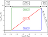 |
Fig. 1. Representation of different models for the effective Reynolds number for the following values: ne = 10−3 cm−3, Re = 100, T = 108 K, vturb = 300 km s−1, vth, i = 1000 km s−1, L0 = 100 kpc, and Bequ = 10−6 G. In the unmagnetized regime, the solid black line is the Reynolds number that is not modified by the regulation of pressure anisotropies and is given in Eq. (25). Between the limiting magnetic field strengths given in Eqs. (1) and (9), we construct the three different models, Models U, M, and L. The black dotted line corresponds to results obtained from simulations of weakly collisional plasmas presented in St-Onge et al. (2020). |
Next we had to establish the equation that governs the evolution and dynamics of the magnetic field. In this work, we assumed that the magnetic field is amplified by the turbulent dynamo, which consists of the stretching, twisting, and folding of the magnetic field lines by turbulent motions (Kazantsev 1968). If we consider the framework of Kolmogorov turbulence, the rate-of-strain tensor is dominated by motions at the viscous scale (Schekochihin & Cowley 2006), which means |∇u|≈(vturb/L0)Re1/2. On the other hand, in a plasma where a Braginskii-type viscosity is assumed, parallel motions to the magnetic field would be damped and only the parallel component of the rate-of-strain tensor  is relevant. Therefore, in using Eq. (6) but replacing Re by Reeff, we obtain
 (27)
(27)
where Reeff depends on the magnetization state and is given in Fig. 1. We solved Eq. (27) for all magnetization states. Once, the magnetic field approaches equipartition with the turbulent velocity field, nonlinear effects should set in and lead to saturation. However, modeling these nonlinear effects is beyond the scope of this work, and we instead simply assumed that the exponential growth ends when the magnetic field reaches the equipartition field strength Bequ.
All in all, we constructed Ntree = 103 merger trees with Nz = 300 steps between z = 0 and zmax. Once plasma parameters are calculated and averaged according to Eqs. (19) and (21), Eq. (27) is solved between two redshift steps. Our choice of time resolution between two given redshift steps is explained in detail in Appendix D.
4. Results
4.1. Basic plasma parameters from 1D profiles
Figure 2 showcases the temporal evolution of various plasma parameters (Sect. 3.3) for different zmax values associated with merger trees generated using the modified GALFORM algorithm. Initially, we observe a similarity in the trends of the temperature and turbulent velocity curves. The algorithm demonstrates a decline in these curves, by approximately 10 to 20% of the total runtime, followed by a local minimum and a subsequent steady increase until it reaches z = 0. Additionally, we notice that higher values of zmax lead to steeper local minima. While the underlying cause of these curve shapes remains unclear, we can provide some explanations. Firstly, it is important to note that the merger trees have been constructed with a uniform mass resolution of Mres = 1012 M⊙, representing a thousandth of the final cluster’s mass. However, the GALFORM algorithm incorporates two stop conditions: reaching a predetermined value of zmax, or the subhaloes reaching the resolution mass during the mass-splitting procedure, regardless of the redshift. Consequently, a higher zmax corresponds to fewer subhaloes in the tree near this redshift. Nonetheless, deviations from the mean values of temperature and turbulent velocity at z = 0 remain minimal. Furthermore, the concentration parameter c is computed at each node of the tree by considering energy conservation, accounting for accreted matter. When the merger tree extends to higher redshift values, the accretion of additional matter can substantially alter the final value of the concentration parameter, which could explain why c values of the curves with 1 ≲ zmax ≲ 2 at z = 0 are higher. However, it is observed from Fig. 2 that variations in c values at z = 0 do not seem to impact the electron density curves. Remarkably, the c value converges to approximately c ≃ 1.2 for z ≳ 2.5, in relatively good agreement with the concentration–mass relation derived in Biviano et al. (2017).
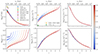 |
Fig. 2. Evolution of various plasma quantities as a function of redshift and for different values of zmax. Each curve represents the average value of the quantity over Ntree = 103 merger trees (see Appendix C) for which a redshift-dependent, one-dimensional profile has been calculated according to Eqs. (19) and (21). The age of the Universe tU at each redshift is plotted on the second x-axis. In order to assess the validity of our model, we added observed values for the temperature and the thermal electron density (see the detailed list in the main text). |
In the preceding paragraph, several concerns regarding the validity of our magnetic field model were raised, as numerical artifacts arise for redshifts close to zmax. As previously stated, both the temperature and turbulent velocity curves exhibit a decreasing trend that precedes a global minimum and then displays a constant increase until z = 0. However, it has been observed that this trend strongly relies on the initial conditions set by zmax, resulting in a numerical effect in our model. In order to mitigate the potential impact of these artifacts on our conclusions, we decided to impose constraints on the value of zmax. Figure 2 clearly indicates that all curves converge toward a common value for redshift values z ≳ 2. Therefore, we opted to exclude merger trees with zmax ≤ 2 for further analysis. Although selecting the merger tree with the highest zmax seems to be a plausible option, it is worth noting that the number of dark matter subhaloes decreases as zmax increases due to the way the GALFORM algorithm operates. Therefore, from now on, we only use the merger tree with zmax = 4 to implement our magnetic field amplification model. Additionally, we initiate the dynamo process at redshift values equal to or below zstart ≤ 2, ensuring that the influence of the mass resolution remains marginal.
Finally, in order to assess the robustness of our model, we plot observational values of various physical quantities for nine different clusters in Fig. 2. It should be noted that this selection of clusters does not include only clusters in the same dynamical state, some are undergoing merging processes, while others are in a relaxed state. For instance, Miranda et al. (2008) combined X-ray observations and strong lensing analysis of RX J1347.5−1145, and revealed a complex structure. They suggested a merger scenario between dark matter subclumps that would account for discrepancies with mass estimates from the virial theorem. Moreover, Barrena et al. (2002) provided evidence of a major collision between 1E 0657−56 and a subcluster, and Maurogordato et al. (2008) provided optical observations suggesting that Abell 2163 had undergone a recent (≈0.5 Gyr) collision. For the temperature, we plotted results from X-ray observations for the Coma cluster, Abell 1795, PKS 0745−19, SW J1557+3530, and SW J0847+1331 from Moretti et al. (2011) and references therein. We also plotted the temperature from X-ray observations from Wallbank et al. (2022) for Abell 2163, Abell 754, RX J1347.5−1145, and 1E 0657−56. Our model results in an average temperature at z = 0, which is in good agreement with most clusters of the observational sample. We also present the thermal electron density values for the Coma cluster, both in its central region and its periphery, at r = r200. These values were obtained from the X-ray morphology Churazov et al. (2021) using the data from SRG/eROSITA. This enables us to assert that the typical plasma values expected at low redshift are overall in accordance with our model.
4.2. Magnetic field amplification
In this section, we present the magnetic field amplification obtained from our model that is based on an effective Reynolds number. It is worth recalling that we integrated our dynamo model into the merger tree with zmax = 4 and initiated the amplification process at various redshifts between zstart = 2 and zstart = 0.1.
4.2.1. Example of magnetic field evolution
Figure 3 shows an example of the magnetic field evolution for the three effective Reynolds number models, detailed in Sect. 3.4, for α0 = 20 (see Eq. (18) for the model of the turbulent forcing scale), zstart = 1.5, and B0 = 10−20 G. The gray curves represent the magnetic field evolution of all individual Ntree = 103 merger trees. In red, we show the skew-normal average median with a 90% confidence interval (see Appendix C). We note that the estimated error during the exponential phase of Model L is larger than that of the other models. This can be partially explained by the fact that, in Model L, kinetic instabilities only modify the Reynolds number once the magnetic field amplitude reaches the order of nG. Compared to Models M and U, in Model L, the Reynolds number remains at a value several orders of magnitude lower for a longer time, allowing the various curves to spread more until the Reynolds number increases drastically, when B exceeds the threshold given by Eq. (9). In all three cases, Fig. 3 demonstrates that once an amplitude of a few nG is achieved, the amplification of the magnetic field toward equipartition is nearly instantaneous.
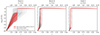 |
Fig. 3. Evolution of magnetic field for α0 = 20 and zstart = 1.5 and for the three models for the effective Reynolds number. The gray curves are the magnetic field evolution of all Ntree = 103 merger trees. The red curve indicates the average obtained by fitting all curves at each redshift value with a skew-normal distribution (see Appendix C). The colored area shows the 90% confidence interval for such a distribution. The age of the Universe tU at each redshift is plotted on the second x-axis. |
Figure 4 illustrates the time evolution of the magnetic field for the three distinct effective Reynolds number models, detailed in Sect. 3.4, for a specific value of α0 = 20, starting at redshifts of zstart = 0.5, 1, and 1.5.
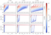 |
Fig. 4. Evolution of magnetic field amplitude over redshift for different models of effective Reynolds number. The curves and shaded areas correspond, respectively, to the average and the 90% confidence interval given by the averaging process described in Appendix C. The age of the Universe tU at each redshift is plotted on the second x-axis. Each row corresponds to a different model, and each column corresponds to a different starting redshift of the dynamo. Model L (top row) has the lowest growth rate, while Models M and U (middle and bottom rows, respectively) show faster growth rates. The figure also shows that the dynamo was much faster in the past (higher redshift values). |
Figure 4 illustrates the same evolution of the magnetic field as Fig. 3, but this time for zstart = 0.5, 1, 1.5 and for initial seed field values ranging from log10(B [G]) = −20 to −10. Firstly, it is evident that for Models M and U, the curves coincide for B0 ≳ 10−16 G and, in particular, the time required to reach equipartition with the turbulent velocity field is independent of B0. Therefore, we chose to omit the error bars in our subsequent analyses described below. It also appears that the growth rate of the magnetic field becomes faster as the redshift increases. This effect can only be justified by the evolution of various plasma parameters incorporated in Eq. (27) for the growth rate.
4.2.2. Time to equipartition
Figure 5 shows the values of redshift zequ at which the magnetic energy density reaches at least 90% of the kinetic energy density of turbulence, for the three models of Reeff, and for different values of α0, B0, and zstart. Figure 6 shows the minimum redshift zmin at which the dynamo has to start such that equipartition with the turbulent velocity field can be reached, for the three effective Reynolds number models and for various values of α0. Firstly, it can be observed that equipartition can be reached in all the different configurations that we implemented. Moreover, it is clear that Models M and U are indistinguishable for log10(B0 [G]) ≳ −17. Furthermore, below these values, the differences between their respective curves are not significant.
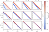 |
Fig. 5. Redshift zequ at which magnetic field reaches at least 90% of equipartition with turbulent velocity field; for different values of initial magnetic seed field. Each row corresponds to the different models of the effective Reynolds number in the magnetized “kinetic” regime (Sect. 3.4). Each column corresponds to a different turbulent injection scale. |
The important conclusions that can be drawn from these results are as follows. Firstly, assuming that the modification of effective ion-ion collisionality is the sole physical quantity modified by kinetic instabilities, it can reasonably be accepted that Model L represents a lower limit of zmin. Additionally, even though Model U does not represent an upper limit to the effective Reynolds number, it can be assumed that any faster model would not result in any changes to the values presented in Fig. 6. In summary, any effective model for the Reynolds number lying between the curves associated with Models M and U would lead to an explosive dynamo so fast that their evolution could not be distinguished with our resolution in redshift. On the other hand, considering a model between the curves L and M would indeed lead to changes in the values of zmin compared to those presented in Fig. 6. Finally, we are limited in the conclusions we can draw due to our simple limitation in modeling the dynamics of the turbulent field, particularly its injection scale. If α0 were to evolve, especially through certain mechanisms of turbulent decay, our results would obviously be modified. We leave a more comprehensive modeling of the turbulent velocity field for future work.
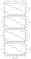 |
Fig. 6. Minimum redshift zmin from which a dynamo has to start to take the magnetic field B0 up to equipartition with the turbulent velocity field at z = 0; for different values of the initial magnetic seed field and for each model for the effective Reynolds number. Each panel corresponds to a specific value of the injection scale defined by Eq. (18). |
5. Discussion
Using merger trees has enabled us to study the evolution of certain plasma quantities, including the magnetic field, without relying on computationally expensive simulations. However, such an approach presents a number of uncertainties. Firstly, we only used the modified GALFORM algorithm, as it was calibrated to the mass function of the Millennium simulations. We do not know (yet) if our conclusions would change when considering another merger tree algorithm.
When applying the merger tree algorithm, we have to pay special attention to numerical artifacts. In particular, we constrained the value of zmax (redshift at which the merging process starts) to zmax = 4, so that our results are not influenced by numerical effects related to mass resolution (see Fig. 2). Furthermore, we decided to start the dynamo process from zstart ≃ 2 or below. Indeed, below zstart = 2, all curves with zmax ≥ 4 are approximately identical. Therefore, our ability to study dynamo processes at z ≳ 2 depends on the model for the concentration parameter considered.
Also, the effective Reynolds number has to be chosen carefully, mainly because Models L and U do not constitute a lower and upper bound per se. This may be susceptible to introducing biases in the minimum redshift, zmin, at which the magnetic field amplification needs to start in order to reach equipartition at z = 0. However, our results have shown that Models M and U produce nearly identical results. This is not surprising, because even if Models M and U are not the same, they both differ from the classical Reynolds number by (many) orders of magnitude.
Furthermore, confining the evolution of the turbulent injection scale appears to be one of the few necessary conditions to constrain the evolution of the magnetic field. It should be noted that other sources of turbulence are likely to exist during certain phases of the formation of a cluster, potentially with different forcing length scales. Other sources include, for example, subcluster and galactic wakes (e.g., Subramanian et al. 2006) and jets from active galactic nuclei (e.g., Fujita et al. 2020).
Finally, for the scenario presented in Fig. 3, for instance, the magnetic field strength increases by 14 orders of magnitude, while the temperature increases by one order of magnitude. In this specific example, the β parameter changes from β ≈ 1028 at z = 1.5 to β ≈ 102 at z = 0. Therefore, we do not expect direct feedback on cluster evolution from the magnetic field through magnetic pressure. However, even at times where β ≫ 1, the strength and direction of the viscosity are affected by the instabilities. This implies that indirect feedback from the magnetic field on the flow can occur, leading to effects that are not captured by classical hydrodynamic simulations (see also the discussion in St-Onge & Kunz 2018).
6. Conclusions
In this work, we used the modified GALFORM code (Parkinson et al. 2008) to investigate the amplification of magnetic fields in the intracluster medium during the formation of galaxy clusters by successive mergers of dark matter halos. We focused on clusters with a typical mass of M = 1015 M⊙.
To this end, we implemented one-dimensional profiles for the distribution of dark matter, baryonic gas, temperature, and turbulent velocity, assuming spherical symmetry and following the methodology proposed by Dvorkin & Rephaeli (2011) and Johnson et al. (2021). For a given merger tree realization, the profiles of all subhalos at a given redshift were averaged in order to calculate relevant plasma parameters as a function of redshift. This process was performed for Ntree = 103 merger trees to establish statistical properties. We compared the temperature at z = 0 obtained from our model with observed values from a sample of selected clusters presented in Moretti et al. (2011) and Wallbank et al. (2022). We also compared the electron density values of our model with SRG/eROSITA observations of the Coma cluster of Churazov et al. (2021). Overall, we found our model to be in good agreement with the observed values from a sample of low-redshift clusters.
We then constructed a semi-analytical model for the amplification of the magnetic field that incorporates the effects of pressure-anisotropy-driven kinetic instabilities (firehose and mirror) for different magnetization regimes (Melville et al. 2016; Rincon et al. 2016; St-Onge & Kunz 2018; St-Onge et al. 2020). Next, we estimated the growth rate of the magnetic field for different values of the strength of the magnetic seed field and forcing length scales of turbulence. This allowed us to determine the redshift at which equipartition is reached in different scenarios. In practice, we define equipartition as the time when the magnetic energy density reaches at least 90% of the turbulent kinetic energy density. Specifically, for an injection scale of L0 = rvir/20, where rvir is the virial radius of the dark matter halo, the magnetic field evolves in the following way: for our slowest dynamo (effect Reynolds number Model L), the dynamo amplification for seed field values of log10(B0 [G]) = −20 and −10 has to start at least from, respectively, zstart ≃ 1 and 0.2 to reach equipartition until the present day. For the other faster scenarios (Models M and U), those values are reduced to zstart ≃ 0.3 and ≃0.1, respectively. Although our Model U cannot be considered an upper limit for the effective Reynolds number, our Model L can constitute a lower limit, provided that the increase of ion-ion collisionality is the sole effect created by the kinetic instabilities to bring the system back to marginal stability.
Overall, our study demonstrates that merger trees can be a valuable tool for constraining the evolution of magnetic fields over cosmological times, especially in galaxy clusters. In particular, they allow us to probe kinetic plasma effects in the history of the ICM that are inaccessible with state-of-the-art cosmological simulations. Although our approach is not as accurate as fully kinetic plasma simulations, it could potentially constitute a computationally efficient alternative for constraining the dependence of the effective Reynolds number on the magnetic field in the magnetic “kinetic” regime when combined with future and more resolved radio observations.
The mirror instability occurs when a magnetic bottle grows in amplitude and is destabilized by an excess of perpendicular pressure over magnetic pressure. The firehose instability is developed when the restoring force of propagating Alfvénic fluctuations is undermined by an opposing viscous stress, making those fluctuations grow exponentially.
This effect could be caused by the combined effects of density stratification and faster eddy turnover time in the ICM’s core.
We note that α0 ≃ 20 is the result obtained in Shi et al. (2018). The last value, α0 = 50, is chosen arbitrarily.
Acknowledgments
We are very grateful to Matthew Kunz and Jonathan Squire for providing us with all the necessary ingredients for modeling magnetic fields in the intracluster medium, during the Nordita program “Magnetic Field Evolution in Low Density or Strongly Stratified Plasmas” in 2022. Undoubtedly, our work would not have been possible without their contribution to the physics of weakly collisional plasmas. We further thank Abhijit B. Bendre for his numerous comments on this study and the referee for a very constructive report. Finally, we acknowledge the support from the Swiss National Science Foundation under Grant No. 185863.
References
- Adshead, P., Giblin, J. T., Jr., Scully, T. R., & Sfakianakis, E. I. 2016, JCAP, 2016, 039 [CrossRef] [Google Scholar]
- Barrena, R., Biviano, A., Ramella, M., Falco, E. E., & Seitz, S. 2002, A&A, 386, 816 [NASA ADS] [CrossRef] [EDP Sciences] [Google Scholar]
- Beck, R., & Wielebinski, R. 2013, in Planets, Stars and Stellar Systems. GalacticStructure and Stellar Populations, eds. T. D. Oswalt, & G. Gilmore, 5, 641 [NASA ADS] [CrossRef] [Google Scholar]
- Beresnyak, A. 2012, Phys. Rev. Lett., 108, 035002 [NASA ADS] [CrossRef] [Google Scholar]
- Bernet, M. L., Miniati, F., Lilly, S. J., Kronberg, P. P., & Dessauges-Zavadsky, M. 2008, Nature, 454, 302 [NASA ADS] [CrossRef] [Google Scholar]
- Biermann, L. 1950, Zeitschrift Naturforschung Teil A, 5, 65 [NASA ADS] [Google Scholar]
- Biviano, A., Moretti, A., Paccagnella, A., et al. 2017, A&A, 607, A81 [NASA ADS] [CrossRef] [EDP Sciences] [Google Scholar]
- Bonafede, A., Feretti, L., Murgia, M., et al. 2010, A&A, 513, A30 [NASA ADS] [CrossRef] [EDP Sciences] [Google Scholar]
- Braginskii, S. I. 1965, Rev. Plasma Phys., 1, 205 [Google Scholar]
- Brandenburg, A., Schober, J., Rogachevskii, I., et al. 2017, ApJ, 845, L21 [NASA ADS] [CrossRef] [Google Scholar]
- Brandenburg, A., Rogachevskii, I., & Schober, J. 2023, MNRAS, 518, 6367 [Google Scholar]
- Chandrasekhar, S., Kaufman, A. N., & Watson, K. M. 1958, Proc. R. Soc. London Ser. A, 245, 435 [NASA ADS] [CrossRef] [Google Scholar]
- Chew, G. F., Goldberger, M. L., & Low, F. E. 1956, Proc. R. Soc. London Ser. A, 236, 112 [NASA ADS] [CrossRef] [Google Scholar]
- Churazov, E., Khabibullin, I., Lyskova, N., Sunyaev, R., & Bykov, A. M. 2021, A&A, 651, A41 [NASA ADS] [CrossRef] [EDP Sciences] [Google Scholar]
- Cole, S., Lacey, C. G., Baugh, C. M., & Frenk, C. S. 2000, MNRAS, 319, 168 [Google Scholar]
- Di Gennaro, G., van Weeren, R. J., Brunetti, G., et al. 2021, Nat. Astron., 5, 268 [Google Scholar]
- Domínguez-Fernàndez, P., Vazza, F., Brüggen, M., & Brunetti, G. 2019, MNRAS, 486, 623 [CrossRef] [Google Scholar]
- Dvorkin, I., & Rephaeli, Y. 2011, MNRAS, 412, 665 [NASA ADS] [CrossRef] [Google Scholar]
- Ellis, J., Fairbairn, M., Lewicki, M., Vaskonen, V., & Wickens, A. 2019, JCAP, 2019, 019 [CrossRef] [Google Scholar]
- Fitzpatrick, R. 2014, Plasma Physics: An Introduction (Taylor& Francis) [CrossRef] [Google Scholar]
- Fujita, T., Namba, R., Tada, Y., Takeda, N., & Tashiro, H. 2015, JCAP, 2015, 054 [CrossRef] [Google Scholar]
- Fujita, Y., Cen, R., & Zhuravleva, I. 2020, MNRAS, 494, 5507 [NASA ADS] [CrossRef] [Google Scholar]
- Gary, S. P. 1992, J. Geophys. Res., 97, 8519 [NASA ADS] [CrossRef] [Google Scholar]
- Gnedin, N. Y., Ferrara, A., & Zweibel, E. G. 2000, ApJ, 539, 505 [NASA ADS] [CrossRef] [Google Scholar]
- Gómez, J. S., Padilla, N. D., Helly, J. C., et al. 2022, MNRAS, 510, 5500 [CrossRef] [Google Scholar]
- Helander, P., Strumik, M., & Schekochihin, A. A. 2016, J. Plasma Phys., 82, 905820601 [NASA ADS] [CrossRef] [Google Scholar]
- Hellinger, P. 2007, Phys. Plasmas, 14, 082105 [NASA ADS] [CrossRef] [Google Scholar]
- Hubrig, S., Schöller, M., Kharchenko, N. V., et al. 2011, A&A, 528, A151 [NASA ADS] [CrossRef] [EDP Sciences] [Google Scholar]
- Jedamzik, K., & Saveliev, A. 2019, Phys. Rev. Lett., 123, 021301 [NASA ADS] [CrossRef] [Google Scholar]
- Johnson, T., Benson, A. J., & Grin, D. 2021, ApJ, 908, 33 [NASA ADS] [CrossRef] [Google Scholar]
- Joyce, M., & Shaposhnikov, M. 1997, Phys. Rev. Lett., 79, 1193 [NASA ADS] [CrossRef] [Google Scholar]
- Kazantsev, A. P. 1968, Sov. J. Exp. Theor. Phys., 26, 1031 [NASA ADS] [Google Scholar]
- Kravtsov, A. V., & Borgani, S. 2012, ARA&A, 50, 353 [Google Scholar]
- Kulsrud, R. M. 1983, in Handbook of Plasma Physics. Basic Plasma Physics I., eds. A. A. Galeev, & R. N. Sudan, 1, 115 [NASA ADS] [Google Scholar]
- Kulsrud, R. M., Cen, R., Ostriker, J. P., & Ryu, D. 1997a, ApJ, 480, 481 [NASA ADS] [CrossRef] [Google Scholar]
- Kulsrud, R., Cowley, S. C., Gruzinov, A. V., & Sudan, R. N. 1997b, Phys. Rep., 283, 213 [NASA ADS] [CrossRef] [Google Scholar]
- Kunz, M. W., Schekochihin, A. A., & Stone, J. M. 2014, Phys. Rev. Lett., 112, 205003 [NASA ADS] [CrossRef] [Google Scholar]
- Marinacci, F., Vogelsberger, M., Pakmor, R., et al. 2018, MNRAS, 480, 5113 [NASA ADS] [Google Scholar]
- Maurogordato, S., Cappi, A., Ferrari, C., et al. 2008, A&A, 481, 593 [NASA ADS] [CrossRef] [EDP Sciences] [Google Scholar]
- McCarthy, I. G., Bower, R. G., & Balogh, M. L. 2007, MNRAS, 377, 1457 [NASA ADS] [CrossRef] [Google Scholar]
- Melville, S., Schekochihin, A. A., & Kunz, M. W. 2016, MNRAS, 459, 2701 [NASA ADS] [CrossRef] [Google Scholar]
- Miniati, F., & Beresnyak, A. 2015, Nature, 523, 59 [NASA ADS] [CrossRef] [Google Scholar]
- Miranda, M., Sereno, M., de Filippis, E., & Paolillo, M. 2008, MNRAS, 385, 511 [NASA ADS] [CrossRef] [Google Scholar]
- Mo, H., van den Bosch, F. C., & White, S. 2010, Galaxy Formation and Evolution (Cambridge: Cambridge University Press) [Google Scholar]
- Mogavero, F., & Schekochihin, A. A. 2014, MNRAS, 440, 3226 [NASA ADS] [CrossRef] [Google Scholar]
- Moretti, A., Gastaldello, F., Ettori, S., & Molendi, S. 2011, A&A, 528, A102 [NASA ADS] [CrossRef] [EDP Sciences] [Google Scholar]
- Naoz, S., & Narayan, R. 2013, Phys. Rev. Lett., 111, 051303 [NASA ADS] [CrossRef] [Google Scholar]
- Navarro, J. F., Frenk, C. S., & White, S. D. M. 1996, ApJ, 462, 563 [Google Scholar]
- Neto, A. F., Gao, L., Bett, P., et al. 2007, MNRAS, 381, 1450 [NASA ADS] [CrossRef] [Google Scholar]
- Ostriker, J. P., Bode, P., & Babul, A. 2005, ApJ, 634, 964 [NASA ADS] [CrossRef] [Google Scholar]
- Parker, E. N. 1958, Phys. Rev., 109, 1874 [NASA ADS] [CrossRef] [Google Scholar]
- Parkinson, H., Cole, S., & Helly, J. 2008, MNRAS, 383, 557 [Google Scholar]
- Planck Collaboration XIX. 2016, A&A, 594, A19 [NASA ADS] [CrossRef] [EDP Sciences] [Google Scholar]
- Planck Collaboration VI. 2020, A&A, 641, A6 [NASA ADS] [CrossRef] [EDP Sciences] [Google Scholar]
- Press, W. H., & Schechter, P. 1974, ApJ, 187, 425 [Google Scholar]
- Quashnock, J. M., Loeb, A., & Spergel, D. N. 1989, ApJ, 344, L49 [NASA ADS] [CrossRef] [Google Scholar]
- Rincon, F. 2019, J. Plasma Phys., 85, 205850401 [NASA ADS] [CrossRef] [Google Scholar]
- Rincon, F., Califano, F., Schekochihin, A. A., & Valentini, F. 2016, Proc. Natl. Acad. Sci., 113, 3950 [NASA ADS] [CrossRef] [Google Scholar]
- Riquelme, M. A., Quataert, E., & Verscharen, D. 2015, ApJ, 800, 27 [NASA ADS] [CrossRef] [Google Scholar]
- Rudakov, L. I., & Sagdeev, R. Z. 1961, Sov. Phys. Dokl., 6, 415 [NASA ADS] [Google Scholar]
- Ryu, D., Kang, H., & Biermann, P. L. 1998, A&A, 335, 19 [NASA ADS] [Google Scholar]
- Santos-Lima, R., de Gouveia Dal Pino, E. M., Kowal, G., et al. 2014, ApJ, 781, 84 [NASA ADS] [CrossRef] [Google Scholar]
- Schekochihin, A. A., & Cowley, S. C. 2006, Phys. Plasmas, 13, 056501 [NASA ADS] [CrossRef] [Google Scholar]
- Schekochihin, A. A., Cowley, S. C., Hammett, G. W., Maron, J. L., & McWilliams, J. C. 2002, New J. Phys., 4, 84 [NASA ADS] [CrossRef] [Google Scholar]
- Schekochihin, A. A., Cowley, S. C., Taylor, S. F., Maron, J. L., & McWilliams, J. C. 2004, ApJ, 612, 276 [NASA ADS] [CrossRef] [Google Scholar]
- Scherrer, P. H., Wilcox, J. M., Svalgaard, L., et al. 1977, Sol. Phys., 54, 353 [NASA ADS] [CrossRef] [Google Scholar]
- Schleicher, D. R. G., Schober, J., Federrath, C., Bovino, S., & Schmidt, W. 2013, New J. Phys., 15, 023017 [NASA ADS] [CrossRef] [Google Scholar]
- Schmassmann, M., Schlichenmaier, R., & Bello González, N. 2018, A&A, 620, A104 [NASA ADS] [CrossRef] [EDP Sciences] [Google Scholar]
- Schober, J., Schleicher, D. R. G., & Klessen, R. S. 2013, A&A, 560, A87 [NASA ADS] [CrossRef] [EDP Sciences] [Google Scholar]
- Schober, J., Rogachevskii, I., & Brandenburg, A. 2022, Phys. Rev. Lett., 128, 065002 [NASA ADS] [CrossRef] [Google Scholar]
- Sharma, P., Hammett, G. W., Quataert, E., & Stone, J. M. 2006, ApJ, 637, 952 [NASA ADS] [CrossRef] [Google Scholar]
- Shi, X., Nagai, D., & Lau, E. T. 2018, MNRAS, 481, 1075 [NASA ADS] [CrossRef] [Google Scholar]
- Snyder, P. B., Hammett, G. W., & Dorland, W. 1997, Phys. Plasmas, 4, 3974 [NASA ADS] [CrossRef] [Google Scholar]
- Southwood, D. J., & Kivelson, M. G. 1993, J. Geophys. Res., 98, 9181 [NASA ADS] [CrossRef] [Google Scholar]
- Springel, V., White, S. D. M., Jenkins, A., et al. 2005, Nature, 435, 629 [Google Scholar]
- St-Onge, D. A. 2019, PhD Thesis, Princeton University, USA [Google Scholar]
- St-Onge, D. A., & Kunz, M. W. 2018, ApJ, 863, L25 [CrossRef] [Google Scholar]
- St-Onge, D. A., Kunz, M. W., Squire, J., & Schekochihin, A. A. 2020, J. Plasma Phys., 86, 905860503 [NASA ADS] [CrossRef] [Google Scholar]
- Subramanian, K., Narasimha, D., & Chitre, S. M. 1994, MNRAS, 271, L15 [NASA ADS] [CrossRef] [Google Scholar]
- Subramanian, K., Shukurov, A., & Haugen, N. E. L. 2006, MNRAS, 366, 1437 [CrossRef] [Google Scholar]
- Talebian, A., Nassiri-Rad, A., & Firouzjahi, H. 2020, Phys. Rev. D, 102, 103508 [NASA ADS] [CrossRef] [Google Scholar]
- Törnkvist, O. 1998, Phys. Rev. D, 58, 043501 [CrossRef] [Google Scholar]
- Tweed, D., Devriendt, J., Blaizot, J., Colombi, S., & Slyz, A. 2009, A&A, 506, 647 [NASA ADS] [CrossRef] [EDP Sciences] [Google Scholar]
- Vazza, F., Roediger, E., & Brüggen, M. 2012, A&A, 544, A103 [NASA ADS] [CrossRef] [EDP Sciences] [Google Scholar]
- Vogt, C., & Enßlin, T. A. 2003, A&A, 412, 373 [NASA ADS] [CrossRef] [EDP Sciences] [Google Scholar]
- Wallbank, A. N., Maughan, B. J., Gastaldello, F., Potter, C., & Wik, D. R. 2022, MNRAS, 517, 5594 [NASA ADS] [CrossRef] [Google Scholar]
- Widrow, L. M. 2002, Rev. Mod. Phys., 74, 775 [NASA ADS] [CrossRef] [Google Scholar]
- Wright, E. L. 2006, PASP, 118, 1711 [NASA ADS] [CrossRef] [Google Scholar]
Appendix A: GALFORM & modified GALFORM models
The GALFORM model (Cole et al. 2000) is based on the extended Press-Schechter theory (Press & Schechter 1974), which considers the following conditional mass function:
 (A.1)
(A.1)
where f(M1|M2) represents the fraction of mass from halos of mass M2 at redshift z2 that is contained in progenitor halos of mass M1 at earlier redshift z1. The parameter δi denotes the linear overdensity threshold for spherical collapse at redshift zi. The quantity σ(M) denotes the rms linear density fluctuation extrapolated at z = 0 in spheres containing mass M. For simplicity, we adopted σi(M)≡σi. Taking the limit z1 → z2, we obtain
 (A.2)
(A.2)
which allows us to find the mean number of halos of mass M1 into which a halo of mass M2 splits when we increase redshift upwards with a redshift step dz1:
 (A.3)
(A.3)
Assuming a resolution mass Mres, we can also determine the average number of progenitors with masses M1 in the interval Mres < M1 < M2/2, which is given by
 (A.4)
(A.4)
along with the fraction of mass of the final object in progenitors below Mres, given by
 (A.5)
(A.5)
The GALFORM algorithm operates as follows. We start with the redshift and the mass of the final halo. Then we consider a redshift step dz1 that satisfies P ≪ 1 (meaning that a halo is unlikely to have more than two progenitors at redshift z + dz). A random number R ∈ [0, 1] is generated. If R > P the main halo is not split, and its mass is reduced to M2(1 − F) to account for the accreted mass. If R ≤ P, then a random mass Mres > M1 > M2/2 is generated to produce two new halos with masses of M1 and M2(1 − F)−M1. The same process is repeated until the maximum redshift or the resolution mass is reached. However, there are some issues with such an approach. One of them is that the conditional mass function (A.1) does not match what is found in N-body simulations. Yet, statistical properties produced by the GALFORM algorithm have similar trends with those of merger trees constructed from high-resolution N-body simulations, with an error on mass progenitors that increases with redshift. In that spirit, Parkinson et al. (2008) replaced the initial statistics Eq. (A.3) with
 (A.6)
(A.6)
where G is a “perturbative” function that matches the generated merger tree with simulations. They also made the following assumption:
 (A.7)
(A.7)
for which they obtained G0 = 0.57, γ1 = 0.38 and γ2 = −0.01. Finally, they obtained halo abundances consistent with the Sheth-Tormen mass function (see Parkinson et al. 2008, and references therein). In our work, we used the same values for G0, γ1, and γ2.
Appendix B: Effect number of generated trees
Figure B.1 shows the effect of the number of generated merger trees, on the skew-normal average (Sect. C) calculated for the temperature, the baryonic gas density, and the turbulent velocity at three different redshifts. The solid horizontal lines correspond to the value calculated with Ntree = 103 merger trees. It is evident that convergence is reached, even for Ntree ≳ 102.5 merger trees. This justifies our choice of setting Ntree = 103.
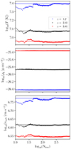 |
Fig. B.1. Skew-normal average of temperature, gas density, and turbulent velocity at three different values of redshift as a function of the number of generated merger trees. The solid lines represent the values of the physical quantities for Ntree = 103. |
Appendix C: Skew-normal averaging process
Here, we present our method for averaging the time evolution curves of all Ntree = 103 merger trees for all physical quantities. Initially, one might consider using the conventional arithmetic average to estimate the overall behavior of these curves at each specific redshift. However, this approach presents a significant flaw when analyzing the evolution of the magnetic field. By examining the left panel of Fig. 3, it becomes evident that at approximately z ≃ 0.75, while a few magnetic field curves have reached equipartition, the majority are still in the phase of exponential growth, with values between B ≈ 10−14 G and B ≈ 10−12 G. Consequently, applying the classical arithmetic average to this dataset would yield a value close to equipartition, which does not accurately represent the actual trend exhibited by all the curves.
We decided to adopt the following strategy. At each given redshift, we fit the distribution of the values of all curves with a skew-normal distribution. However, special attention has to be paid to the magnetic field, as shown in Fig. C.1. Here, we show the histograms of different quantities, where the y-axis is normalized so that the total area of the histogram equals one. The top panel shows the temperature distribution at redshift z = 0.29, and the middle one shows the distribution of the magnetic field at the same redshift. If we were to fit the whole magnetic field sample, a skew-normal distribution would not necessarily be suitable as two distinct maxima appear. Therefore, we adopted the following convention. Whenever the number of trees that have reached equipartition is dominant, we fit the region delimited by dashed lines on the middle panel, which is shown on the bottom panel. However, if this number is smaller than the trees outside this region, we fit the trees in the latter. Finally, we note that the situation where the two histograms, distinguishing the equipartition magnetic field from other values, have the same number of occurrences is extremely rare.
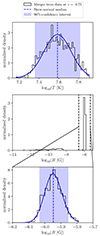 |
Fig. C.1. Illustration of our method using a skew-normal distribution to average different physical quantities at a given redshift, for many merger trees. (top) Distribution of the temperature values from all merger trees at redshift z = 0.75. The blue line represents the skew-normal distribution used to fit the data. The dashed line and the blue-shaded line, respectively, are the distribution’s median (that is used as an estimator for the average of all curves) and its corresponding 90% confidence interval. (middle) Distribution of magnetic field values at this same redshift. The two dashed black lines indicate the region that is fit with the skew-normal distribution. (bottom) Fitting within the region in the middle panel. Those three panels were computed with Reeff Model L, for log10(B0 [G]) = −20, α0 = 20, and zstart = 1.5. |
Appendix D: Time resolution of the dynamo model
As described in Sect. 3.4, we solved Eq. (27) between every redshift step of our merger tree (we recall that Nz = 300). Redshift is converted to time using the cosmology calculator of Wright (2006) with the cosmological parameters given in Sect. 3.1. However, considering only the two values of time between two redshift steps is not efficient enough to highlight the complexity of the different stages of the dynamo, such as nonlinear effects when the magnetic field is approaching equipartition. Therefore, we created a discretized time grid, between two given redshift steps, whose time step is kept constant (meaning that the number of time grid cells between two different consecutive reshifts will vary). The constant time step is given as follows. We can see that Eq. (27) is of the form B(t)∝eΓefft, where  is the growth rate of the magnetic field. However, given our construction for the effective Reynolds number in Sect. 3.4, it is obvious that Reeff ≥ Re, which would yield a smaller timescale of the growth rate than with the classical Reynolds number. Therefore, in order to avoid over-discretizing our grid, we considered the timescale coming from the classical Reynolds number, Γ−1, to be a minimum timescale that should not be exceeded. Therefore, the constant value Δt of all grid cells NΔt contained in our discretized time between two redshift steps is given by
 (D.1)
(D.1)
where αB is a constant value.
We determine the latter by plotting the evolution of the magnetic field, for a fixed set of merger-tree parameters, and for different values of αB. Figure D.1 shows such results for B0 = 10−15 G and α0 = 20. It appears that when αB ≈ 103.5, all curves converge. Therefore, in our work, we adopted a constant value of αB = 104. We note that we checked that this value of αB does not produce other results for all other parameters of B0 and α0.
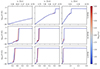 |
Fig. D.1. Magnetic field evolution for different values of αB. Each column corresponds to a different value of redshift at which the dynamo starts. Each row corresponds to a different model for the effective Reynolds number described in Sect. 3.4. |
Appendix E: Estimation of the c parameter
We describe our method to determine the concentration parameter in every subhalo of the generated merger trees here. We started by initiating a value of c for subhalos at zmax, with
 (E.1)
(E.1)
which was proposed by Neto et al. (2007) and where h is the Hubble constant in units of 100 km s−1 Mpc−1 (see Springel et al. 2005). This choice of the initial condition given in Eq. E.1 is somehow arbitrary, but after trying different values of c for the earliest halos, we found that the final result does not depend on this particular choice. We calculated the total energy of every subhalo using the same expressions adopted in Johnson et al. (2021), which is the sum of its kinetic and potential energy, given, respectively, by
![Mathematical equation: $$ \begin{aligned} T = 2\pi \left[r_{\mathrm{vir} }^3\rho (r_{\mathrm{vir} })\sigma ^2(r_{\mathrm{vir} })+\int _{0}^{r_{\mathrm{vir} }}GM(r)\rho (r) r \mathrm{d}r\right] \end{aligned} $$](/articles/aa/full_html/2024/03/aa47497-23/aa47497-23-eq48.gif) (E.2)
(E.2)
and
![Mathematical equation: $$ \begin{aligned} W = -\frac{G}{2}\left[\int _0^{r_{\mathrm{vir} }}\frac{M^2(r)}{r^2} \mathrm{d}r + \frac{M^2(r_{\mathrm{vir} })}{r_{\mathrm{vir} }}\right]. \end{aligned} $$](/articles/aa/full_html/2024/03/aa47497-23/aa47497-23-eq49.gif) (E.3)
(E.3)
Here, σ(r) is the velocity dispersion that is determined by the Jeans equation:
 (E.4)
(E.4)
Therefore, each halo was attributed a total energy of Eh = T + W, which depends on parameters ρs and rs. When a subhalo was the result of N merging subhalos, we computed the energy Eh, f = Tf + Wf of the resulting halo, which we equalized with the energy of the system of all progenitors. We expressed the total energy EN of a system of N subhalos using the same strategy presented in Dvorkin & Rephaeli (2011), which is
 (E.5)
(E.5)
where
 (E.6)
(E.6)
is the gravitational energy of two halos at the largest point of their separation, with d0, ij being the distance at which subhalos i and j are bound, and where
 (E.7)
(E.7)
is the energy component of the accreted matter; rvir, f stands for the virial radius of the resulting halo, and ΔM ≡ Mf − ∑iMi is the mass that was not resolved during the merging event, below the value of Mres. We used the same value of d0 as the one adopted in Dvorkin & Rephaeli (2011), which is d0, ij = 5(rvir, i + rvir, j). Our strategy was then to compute the energy for each subhalo (whether it has one or multiple progenitors) and find the value of c that matches the energy conservation with its progenitors. Once c was calculated, the parameter ρs was obtained by integrating the dark matter density to match the mass of each subhalo.
All Figures
|
Fig. 1. Representation of different models for the effective Reynolds number for the following values: ne = 10−3 cm−3, Re = 100, T = 108 K, vturb = 300 km s−1, vth, i = 1000 km s−1, L0 = 100 kpc, and Bequ = 10−6 G. In the unmagnetized regime, the solid black line is the Reynolds number that is not modified by the regulation of pressure anisotropies and is given in Eq. (25). Between the limiting magnetic field strengths given in Eqs. (1) and (9), we construct the three different models, Models U, M, and L. The black dotted line corresponds to results obtained from simulations of weakly collisional plasmas presented in St-Onge et al. (2020). |
| In the text | |
|
Fig. 2. Evolution of various plasma quantities as a function of redshift and for different values of zmax. Each curve represents the average value of the quantity over Ntree = 103 merger trees (see Appendix C) for which a redshift-dependent, one-dimensional profile has been calculated according to Eqs. (19) and (21). The age of the Universe tU at each redshift is plotted on the second x-axis. In order to assess the validity of our model, we added observed values for the temperature and the thermal electron density (see the detailed list in the main text). |
| In the text | |
|
Fig. 3. Evolution of magnetic field for α0 = 20 and zstart = 1.5 and for the three models for the effective Reynolds number. The gray curves are the magnetic field evolution of all Ntree = 103 merger trees. The red curve indicates the average obtained by fitting all curves at each redshift value with a skew-normal distribution (see Appendix C). The colored area shows the 90% confidence interval for such a distribution. The age of the Universe tU at each redshift is plotted on the second x-axis. |
| In the text | |
|
Fig. 4. Evolution of magnetic field amplitude over redshift for different models of effective Reynolds number. The curves and shaded areas correspond, respectively, to the average and the 90% confidence interval given by the averaging process described in Appendix C. The age of the Universe tU at each redshift is plotted on the second x-axis. Each row corresponds to a different model, and each column corresponds to a different starting redshift of the dynamo. Model L (top row) has the lowest growth rate, while Models M and U (middle and bottom rows, respectively) show faster growth rates. The figure also shows that the dynamo was much faster in the past (higher redshift values). |
| In the text | |
|
Fig. 5. Redshift zequ at which magnetic field reaches at least 90% of equipartition with turbulent velocity field; for different values of initial magnetic seed field. Each row corresponds to the different models of the effective Reynolds number in the magnetized “kinetic” regime (Sect. 3.4). Each column corresponds to a different turbulent injection scale. |
| In the text | |
|
Fig. 6. Minimum redshift zmin from which a dynamo has to start to take the magnetic field B0 up to equipartition with the turbulent velocity field at z = 0; for different values of the initial magnetic seed field and for each model for the effective Reynolds number. Each panel corresponds to a specific value of the injection scale defined by Eq. (18). |
| In the text | |
|
Fig. B.1. Skew-normal average of temperature, gas density, and turbulent velocity at three different values of redshift as a function of the number of generated merger trees. The solid lines represent the values of the physical quantities for Ntree = 103. |
| In the text | |
|
Fig. C.1. Illustration of our method using a skew-normal distribution to average different physical quantities at a given redshift, for many merger trees. (top) Distribution of the temperature values from all merger trees at redshift z = 0.75. The blue line represents the skew-normal distribution used to fit the data. The dashed line and the blue-shaded line, respectively, are the distribution’s median (that is used as an estimator for the average of all curves) and its corresponding 90% confidence interval. (middle) Distribution of magnetic field values at this same redshift. The two dashed black lines indicate the region that is fit with the skew-normal distribution. (bottom) Fitting within the region in the middle panel. Those three panels were computed with Reeff Model L, for log10(B0 [G]) = −20, α0 = 20, and zstart = 1.5. |
| In the text | |
|
Fig. D.1. Magnetic field evolution for different values of αB. Each column corresponds to a different value of redshift at which the dynamo starts. Each row corresponds to a different model for the effective Reynolds number described in Sect. 3.4. |
| In the text | |
Current usage metrics show cumulative count of Article Views (full-text article views including HTML views, PDF and ePub downloads, according to the available data) and Abstracts Views on Vision4Press platform.
Data correspond to usage on the plateform after 2015. The current usage metrics is available 48-96 hours after online publication and is updated daily on week days.
Initial download of the metrics may take a while.