| Issue |
A&A
Volume 673, May 2023
|
|
|---|---|---|
| Article Number | A47 | |
| Number of page(s) | 26 | |
| Section | Extragalactic astronomy | |
| DOI | https://doi.org/10.1051/0004-6361/202244753 | |
| Published online | 03 May 2023 | |
Numerical dependencies of the galactic dynamo in isolated galaxies with SPH
Institute of Theoretical Astrophysics, University of Oslo, Postboks 1029, 0315 Oslo, Norway
e-mail: robertwi@astro.uio.no; sijing.shen@astro.uio.no
Received:
16
August
2022
Accepted:
27
February
2023
Simulating and evolving magnetic fields within global galaxy simulations provides a large tangled web of numerical complexity due to the vast amount of physical processes involved. Understanding the numerical dependencies that act on the galactic dynamo is a crucial step in determining what resolution and conditions are required to properly capture the magnetic fields observed in galaxies. Here, we present an extensive study on the numerical dependencies of the galactic dynamo in isolated spiral galaxies using smoothed particle magnetohydrodynamics. We performed 53 isolated spiral galaxy simulations with different initial setups, feedback, resolution, Jeans floor, and dissipation parameters. The results show a strong mean-field dynamo occurring in the spiral-arm region of the disk, likely produced by the classical alpha-omega dynamo or the recently described gravitational instability dynamo. The inclusion of feedback is seen to work in both a destructive and positive fashion for the amplification process. Destructive interference for the amplification occurs due to the breakdown of filament structure in the disk, the increase of turbulent diffusion, and the ejection of magnetic flux from the central plane to the circumgalactic medium. The positive effect of feedback is the increase in vertical motions and the turbulent fountain flows that develop, showing a high dependence on the small-scale vertical structure and the numerical dissipation within the galaxy. Galaxies with an effective dynamo saturate their magnetic energy density at levels between 10 and 30% of the thermal energy density. The density-averaged numerical Prandtl number is found to be below unity throughout the galaxy for all our simulations, with an increasing value with radius. Assuming a turbulent injection length of 1 kpc, the numerical magnetic Reynolds number is within the range of Remag = 10 − 400, indicating that some regions are below the levels required for the small-scale dynamo (Remag, crit = 30 − 2700) to be active.
Key words: galaxies: evolution / galaxies: magnetic fields / methods: numerical / galaxies: spiral / dynamo / magnetohydrodynamics (MHD)
© The Authors 2023
 Open Access article, published by EDP Sciences, under the terms of the Creative Commons Attribution License (https://creativecommons.org/licenses/by/4.0), which permits unrestricted use, distribution, and reproduction in any medium, provided the original work is properly cited.
This article is published in open access under the Subscribe to Open model. Subscribe to A&A to support open access publication.
1. Introduction
Observations in the last few decades have revealed that many galaxies exhibit strong magnetic fields, with strengths from around several μG for the Milky Way and nearby galaxies (Opher et al. 2009; Fletcher 2010; Burlaga et al. 2013; Beck 2015) up to several mG in starburst galaxies (Chyży & Beck 2004; Robishaw et al. 2008; Heesen et al. 2011; Adebahr et al. 2013). The magnetic energy in these galaxies is found to be close to equipartition with the thermal and turbulent energies (Boulares & Cox 1990; Beck et al. 1996; Taylor et al. 2009), meaning that they are strong enough to dynamically affect the galaxy. Furthermore, it has been observed that the morphology of the magnetic field within disk galaxies exhibits a large-scale spiral structure (Beck & Wielebinski 2013). In disk galaxies with a strong density wave structure, the magnetic field tightly coincides with the optical spiral arms, as in M 51 and M 83 with a strength of around 20 − 30 μG (Fletcher et al. 2011; Frick et al. 2016). For galaxies with a weaker density structure, the magnetic field can instead form large-scale magnetic arms not coinciding with the optical spiral arms, such as in NGC 6946 (Beck 2007).
The strong magnetic fields observed can contribute a significant nonthermal pressure component to the galaxy, which can suppress star formation rates and heavily affect the structure of the interstellar medium (ISM; Pakmor & Springel 2013; Birnboim et al. 2015). The correlation between the star formation rate density and the magnetic field strength has been measured from observations to be between B ∝ SFR0.18 (Chyży et al. 2007) and B ∝ SFR0.3 (Heesen et al. 2014). Within the ISM the magnetic field also plays an important role in the dynamics of molecular clouds, where strong fields can lead to more massive but fewer cloud cores (Vázquez-Semadeni et al. 2005; Price & Bate 2008). Another interesting aspect of magnetic fields within galaxies is that they can suppress the development of fluid instabilities (Jun et al. 1995; McCourt et al. 2015). This can allow for cold gas to survive longer within the predominately hot galactic outflows. This could provide a possible explanation for the significant observational component of cold molecular gas seen in galactic outflows (Chen et al. 2010; Cicone et al. 2014; Leroy et al. 2015; Martini et al. 2018). The strength and structure of magnetic fields in galaxies also determine the transport of cosmic rays (CRs), which together with magnetic fields can efficiently drive galactic outflows (Uhlig et al. 2012; Booth et al. 2013; Pakmor et al. 2016; Butsky & Quinn 2018).
The magnetic fields in galaxies are thought to originate from weak initial seed fields that are rapidly amplified in time by the galactic dynamo. There are several possible origins for the initial seed field, such as through the Biermann battery (Hanayama et al. 2005), from shock and ionization fronts (Subramanian et al. 1994), from plasma instabilities (Bisnovatyi-Kogan et al. 1973; Rees 2005; Lazar et al. 2009; Schlickeiser 2012; Schlickeiser & Felten 2013), from a primordial origin (Durrer & Neronov 2013). Additional seed fields can also be injected into the ISM through stellar winds, supernova (SN), and active galactic nucleus (AGN) feedback. These initial seed fields can potentially be very weak, for example, the Biermann battery process is estimated to generate fields on the order of 10−20 G. This would require the galactic dynamo to amplify the seed field by more than 14 orders of magnitude to replicate the current observed magnetic field strength of nearby galaxies. In addition, observations indicate that strong fields were already in place at high redshift (Widrow 2002; Bernet et al. 2008). The turbulent medium of galaxies gives rise to two distinct groups of dynamo processes that can achieve these sorts of growth rates. The first is the small-scale fluctuating dynamo, which can occur in any turbulent system as it is driven by the random stretching, twisting, and folding of the field lines. This produces randomly oriented magnetic fields at scales smaller than the injection scale of turbulence. As the most rapid stretching, twisting, and folding happens on small scales, the e-folding time is set by the turnover time of the viscous-scale eddies, giving analytical e-folding times predicted to be less than 10 − 100 Myr for galaxies (Schekochihin et al. 2004). The small-scale dynamo eventually saturate when the field becomes sufficiently strong to back-react on the flow and hinder the twisting of the field. The other group of dynamo processes are the mean-field dynamos, which generate magnetic fields at higher scales than the injection scale of turbulence. This requires that the underlying turbulence interacts with larger-scale inhomogeneities in the density or flow structure, for example with shearing flows and density stratification. This causes larger-scale polarities to appear in the magnetic field.
The turbulence in the ISM is continuously regenerated by various stirring mechanisms, which include SN explosions and stellar winds (McKee 1989; Balsara et al. 2004; de Avillez & Breitschwerdt; Krumholz et al. 2006; Gritschneder et al. 2009; Breitschwerdt et al. 2009; Peters et al. 2011; Lee et al. 2012; Kim & Ostriker 2015; Smith et al. 2021; Bieri et al. 2022), gravitational collapse and accretion (Hoyle 1953; Klessen & Hennebelle 2010; Elmegreen & Burkert 2010; Vázquez-Semadeni et al. 2010; Federrath et al. 2011b; Robertson & Goldreich 2012), AGN feedback (Mukherjee et al. 2016), spiral-arm compression (Dobbs & Bonnell 2008; Dobbs 2008), cloud-cloud collisions (Tasker & Tan 2009; Benincasa et al. 2013), the magneto-rotational instability (Piontek & Ostriker 2007; Tamburro et al. 2009), and the galactic shearing flows. This means that the small-scale dynamo is likely active active within the ISM. However, the efficiency and saturation of the small-scale dynamo heavily depends on the fluid parameters (Reynolds number, magnetic Reynolds number, Prandtl number, and Mach number) and the mixtures of solenoidal-to-compressible modes within the turbulent flow (Federrath et al. 2014).
Turbulence can be decomposed into two modes, compressive (potential) modes (∇ × v = 0) and solenoidal (rotational) modes (∇ ⋅ v = 0). Different turbulence driving mechanisms can excite more or less of either mode. Feedback processes such as SN explosions and gravitational collapse are compressive drivers and mainly inject compressive modes within the fluid, while the magneto-rotational instability and shearing flows are solenoidal drivers that mainly inject solenoidal modes. While these drivers initially inject a certain mode, each mode can feed on the other as they interact with their environment (Sasao 1973). This is important as turbulence containing only compressive modes cannot directly excite the small-scale dynamo as it does not impart any vorticity to the fluid (thereby no twisting and folding of the field lines; Mee & Brandenburg 2006). However, indirectly through significant transfer between compressional modes to solenoidal modes, the dynamo can be excited, for example through nonlinear interactions of colliding shocks (Vishniac 1994; Sun & Takayama 2003; Kritsuk et al. 2007; Federrath et al. 2010), rotation and shear forces (Del Sordo & Brandenburg 2011), baroclinicity (Padoan et al. 2016), and through viscous forces (Mee & Brandenburg 2006; Federrath et al. 2011a). The developed/saturated ratio of solenoidal to compressional modes is thus a complicated matter which heavily depends on the fluid conditions and environment.
If we take the turbulence in the ISM as an example, which is highly supersonic at Mach numbers of around 10−100 (Mac Low & Klessen 2004), we can see that this environment generates significant energy transfer between compressional and solenoidal modes, and this can significantly affect the dynamo process. This works both ways, with coherent vortex structures being destroyed by the formation of shocks (Haugen et al. 2004a), and vorticity being generated in the interaction of oblique colliding shocks (Sun & Takayama 2003; Kritsuk et al. 2007). As shown by Federrath et al. (2010), the balance between these two processes is highly dependent on the Mach number, where at higher Mach numbers vorticity generation was shown to become the dominant factor.
In the case of numerical simulations, we can potentially fail to resolve the energy transfer between modes due to resolution constraints. An interesting example illustrating this can be seen in the works Federrath et al. (2011b) and Turk et al. (2012), which showed that to properly resolve the ratio of solenoidal-to-compressional turbulence generated in gravitational collapse (roughly Esol/Etot = 2/3), the local Jeans length was required to be resolved by a high enough number of resolution elements (30 in Federrath et al. 2011b and 64 in Turk et al. 2012). Below this resolution requirement, the compressional modes injected at the Jeans length will fail to properly be converted to solenoidal modes at smaller scales. For the small-scale dynamo, this is significant, as the magnetic field amplification below this resolution criteria showed no growth or a reduction in the field strength (relative to the spherical adiabatic compression of the field lines B ∝ ρ2/3). It is still somewhat uncertain how resolution and different numerical schemes affect the transfer mechanisms mentioned above.
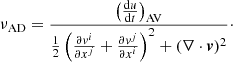
Another big factor for the dynamo relates to the injection length of these turbulent drivers, as this is the scale, together with the velocity and dissipation parameters, determining what the efficient Reynolds numbers and magnetic Reynolds number are in the simulation

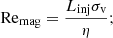
here Linj is the injection scale, σv is the turbulent velocity dispersion on that length scale, ν is the viscosity coefficient, and η is the resistivity coefficient. The growth of the turbulent dynamo strongly depends on these two parameters, where higher numbers generally lead to faster growth of the magnetic field. The so-called critical magnetic Reynolds number can be seen to represent the minimum separation required between the injection scale and the dissipative scales to drive the small-scale dynamo. The critical magnetic Reynolds number depends on both the fluid environment (shear, rotation, and compressibility) and the Reynolds number, and it remains fairly uncertain. Values of around Remag = 30 − 2700 are given from different model analyses and numerical simulations of turbulent systems (Haugen et al. 2004b; Brandenburg & Subramanian 2005; Schober et al. 2012; Federrath et al. 2014). While the range of values are fairly large, there is a tendency for higher critical magnetic Reynolds number for higher compressibility. The different turbulence drivers that we discussed earlier will all have different injection lengths, some more global (e.g., spiral-arm compression and shear) and others more local (e.g., SN and AGN feedback, as well as collapse). The turbulence injection length of SN feedback in a simulation heavily depends on the subgrid model and the environment in the ISM. This remains fairly unexplored for the smoothed particle hydrodynamics (SPH) subgrid models, so it is hard to give a good estimate. High-resolution ISM simulations with grid codes have shown that SNe have injection scales of roughly 60−200 pc (Joung & Mac Low 2006; de Avillez & Breitschwerdt 2007; Gent et al. 2013; Hollins et al. 2017), which include simulations with and without SN clustering. This is smaller than the average size of superbubbles from SN clustering, which lies between 0.5 and 1 kpc. The reason given for the small injection scale is that local breakup of bubbles occurs earlier in the ISM due to the strong density and pressure gradients present. Still, this is using high-resolution local simulations, and it is not necessary that this correlates to the same scale for our subgrid models of stellar feedback. On the other hand, turbulent injection from spiral arm compression and breakdown occurs on much larger scales (1−3 kpc). Even larger turbulence injection occurs through accretion flows onto the disk. Potentially there can also be larger shear turbulence introduced between the disk and the circumgalactic medium (CGM). The small-scale dynamo of the ISM is predicted to saturate the magnetic field with energies at around 1 − 50% of equipartition with the turbulent energy (Schekochihin et al. 2005).
While the small-scale dynamo gives a mechanism that can quickly amplify the field, it is more uncertain whether the same mechanism can generate the large-scale fields observed in galaxies. The difficulty lies in that a small-scale dynamo produces random-oriented fields below the turbulent injection scale. If the turbulent injector occurs on scales larger than the ISM scale, the small-scale dynamo can produce coherent ISM scale fields, as fields can become correlated in accretion flows (Rieder & Teyssier 2017b; Vazza et al. 2018). However, for ISM-scale turbulent injectors (such as SNe), we require magnetic energy to be transferred from small-scale (below injection length) to large scales. A possible mechanism for this inverse cascade is the self-assembly of the magnetic field in regions of turbulent relaxation, where turbulence is not actively driven (Frisch et al. 1975; Alexakis et al. 2006; Zrake 2014; Brandenburg et al. 2015). In this process, the fluctuating small-scale fields generated from a small-scale dynamo start to merge into larger coherent fields. Another possibility to generate these large-scale fields is through the mean-field dynamo. The most well-known mean-field dynamo is the classical αΩ dynamo, which depends on the shear of the flow (Ω effect) and the small-scale velocity helicities in the flow (α effect). However, the αΩ dynamo is plagued by the so-called catastrophic-quenching effect1, which effectively limits the saturation strength of the large-scale magnetic fields. The saturation can be shown to be proportional to 1/Remag, which for the ISM Remag ≈ 1015 results in very low saturation levels (Blackman & Brandenburg 2002; Brandenburg & Subramanian 2005). This is only true if one assumes that the helicity within active dynamo regions is conserved (closed boundary). However, in galaxies there are plenty of processes that can remove helicity from the disk and thus quenching can be avoided (Brandenburg & Sandin 2004). The growth rate of the αΩ effect strongly depends on both the global properties of the disk (scale height, shear parameter, etc.) and the small-scale properties (injection length, dissipation, etc.). Similarly, there is also the α2 dynamo, which solely relies on the small-scale velocity helicities in the flow to generate its mean field and it may be an important process in generating mean fields in galaxies with more uniform rotation (Brandenburg & Subramanian 2005).
Another type of mean-field dynamo that has recently emerged as a very interesting prospect for dynamo growth within astrophysical disks is the gravitational-instability (GI) dynamo (Riols & Latter 2019). This is a dynamo that is sustained by the gravito-turbulence injected during spiral arm compression, which generates vertical rotating flow rolls. During compression, the toroidal field is pinched, lifted, and folded by these flow rolls, generating new radial fields. These radial fields are then sheared by the differential rotation generating toroidal fields, closing the dynamo loop. This is similar to the αΩ-type dynamo, but slightly different as it is governed by larger-scale motions than the turbulent helical motions. The growth rate of this dynamo strongly depends on the cooling rate and the effective Reynolds number. The critical Reynolds number has been shown to be around the order of unity (Remag, crit = 4 for τc = 20Ω−1, where τc is the cooling time and Ω is the rotation rate). Above this value, the dynamo starts to saturate close to quasi-equipartition with the turbulent energy, but it shows a decrease in saturation above Remag ≥ 100. In Riols & Latter (2019), high Remag ≥ 100 simulations show an increased small-scale structure in the large-scale magnetic ropes inside spiral waves. It is suggested that the small-scale fields were generated by the turbulent small-scale dynamo which can act to break down the large-scale field through parasitic (secondary) instabilities. This would be similar to the breakdown of channel modes for the MRI and reminiscent of the “catastrophic-quenching effect” for the αΩ effect. However, as of yet, there has not been an extensive study of higher Remag simulations looking at this dynamo, making its behavior in this regime difficult to predict.
Apart from the αΩ effect and the GI dynamo, there are several other proposed mechanisms that can develop coherent large-scale magnetic fields in galaxies, for example the cosmic-ray-driven dynamo (Lesch & Hanasz 2003; Hanasz et al. 2009), the shear-current effect (Rogachevskii & Kleeorin 2003, 2004; Squire & Bhattacharjee 2015), and the stochastic alpha effect (Vishniac & Brandenburg 1997; Silant’ev 2000; Heinemann et al. 2011). However, it remains unexplored if any of these additional mechanisms can lead to a sustained dynamo in a more realistic environment with global and open boundary conditions.
A natural way to study both the small-scale and large-scale dynamo in galaxies is through numerical simulations. There have been great advances in the understanding and numerical modeling of galaxies through the inclusion of physical processes such as the gravitational interaction between dark matter, stars, and gas (Aarseth & Fall 1980; Stadel 2001; Dehnen 2002); the hydrodynamic modeling of gas (Teyssier 2002; Wadsley et al. 2004; Springel 2010); the formation of stars (Katz 1992); the feedback and output from SNe and stellar winds (Katz 1992; Springel & Hernquist 2003); the feedback and output from black holes (Di Matteo et al. 2005); and the radiative cooling of gas (Marri & White 2003; Shen et al. 2010). With this physics included, cosmological simulations are able to reproduce many observables in galaxies. However, magnetic fields still remain one of the most often neglected parts, mostly due to the complexity and technical difficulties associated with them. As we have seen, the magnetic field is closely interwoven with the dynamical state of the galaxy. The environment determines the growth of the magnetic field, which in turn has an effect on the dynamics. This means that there can be strong dependencies between the magnetic field and the other different physical processes (e.g., star formation, SN explosion, radiation transport, AGN). These strong dependencies become clear when we look at previous simulations of galaxies with magnetic fields, which have been shown to produce a wide range of different magnetic field amplification and saturations. Some show magnetic fields growing up to levels near equipartition with the turbulent energy (Wang & Abel 2009; Pakmor & Springel 2013; Butsky et al. 2017), while others end up with a relatively weak saturated field (Rieder & Teyssier 2017a; Su et al. 2018; Martin-Alvarez et al. 2018)
There are also numerical difficulties to consider when modeling the magnetic field within galaxies. First of all, in numerical simulations, the smallest spatial scale that we resolved is restricted by the number of resolution elements that we could afford to use in the computation. This is clearly relevant for magnetic fields, as the dynamo processes mentioned above are heavily dependent on the small-scale dissipation of the system. Apart from the independent dissipation of the magnetic and kinetic energies, amplification of the magnetic field has also been shown to be heavily dependent on the ratio between the magnetic and kinetic dissipation, otherwise known as the magnetic Prandtl number. This ratio is often overlooked in numerical simulations, but is crucial to understand the amplification and saturation of the magnetic field (Schekochihin et al. 2004; Brandenburg & Subramanian 2005; Wissing et al. 2022). In nature, galaxies are expected to have magnetic Prandtl numbers far greater than unity (in molecular clouds Pm ≈ 1010; Federrath 2016). In numerical simulations, the numerical Prandtl number is set by the numerical dissipation scheme used for the velocity and magnetic fields. For grid code, the Prandtl number remains fairly constant at around Pm = 2 (Fromang et al. 2007; Lesaffre & Balbus 2007; Simon et al. 2009; Federrath et al. 2011a), though these estimates are taken for subsonic flow and might change for supersonic flows. For SPH, this ratio is more resolution dependent as seen in Wissing et al. (2022) and Tricco et al. (2016b) and lies somewhere between Pm = 1 − 2 for subsonic flow2.
Another technical consideration involves the generation of unphysical divergence errors (magnetic monopoles), due to truncation errors in the numerical discretization and integration of the magnetohydrodynamic (MHD) equations. Large divergence errors can lead to both force errors and amplification errors for the magnetic field. It is therefore crucial to try to keep the divergence error as close to zero as possible. Galaxy simulations prove to be one of the more difficult simulations in regards to withholding the divergence constraint, due to the supersonic environment, shear, open boundaries, and the large amount of subgrid recipes. However, in the last few decades, there have been tremendous improvements in reducing and handling these errors within numerical simulations. In Eulerian codes, the divergence-free constraint can be enforced to machine precision with the constrained transport method (Evans & Hawley 1988). This is not easily applicable for Lagrangian codes3. However, improved divergence cleaning methods have been developed that can significantly reduce the error for SPH (Tricco & Price 2012; Tricco et al. 2016a).
In this paper, we study in detail how different numerical parameters such as SN feedback, resolution, Jeans floor, diffusion parameters, and initial conditions affect the growth and saturation of the magnetic field. This paper is organized as follows. In Sect. 2, we go through the simulation setup and the post-process analysis. In Sect. 3, we present our result. In Sect. 4, we discuss our results and present some concluding remarks.
2. Simulation description
2.1. Simulation setup
For all our simulations we use the MHD version of GASOLINE2 with the same default set of code parameters as in Wissing & Shen (2020), except number of smoothing neighbors set to Nneigh = 64. GASOLINE2 applies different gradient operators compared to traditional SPH (TSPH)4 which has shown to improve solutions near density discontinuities (Wadsley et al. 2017). In particular, when applied to the magnetized cloud collapse, jet formation was captured at lower resolutions and for weaker magnetic fields compared to previous SPH+MHD schemes (Wissing & Shen 2020). Additionally, GDSPH was able to successfully capture the development of the magnetorotational instability in a stratified medium, whereas previous meshless methods either developed numerical instability or saw decay of the turbulence after a short period of time (Deng et al. 2019; Wissing et al. 2022). The non-MHD version of GASOLINE2 has moreover been widely used to study galaxy formation in large-scale cosmological boxes, cosmological zoom-in simulations and isolated galaxy simulations.
For our initial conditions (ICs) we use the isolated disk galaxy from the AGORA comparison project (Kim et al. 2014), which was modeled to be similar to a Milky-Way type galaxy at z = 0. The IC was generated by the MAKEDISK code (Springel et al. 2005), which distributes the particles provided an equilibrium solution to the Jeans equation for a multicomponent system including the halo, disk, and bulge. The initial gas metallicity is set to solar values. This IC is very useful as it has been readily used in the literature, which allows for more comparison to our simulations. The AGORA comparison project offers several resolutions of this disk galaxy, for our simulations we split all the particles of the lowest resolution AGORA IC by 8 times (low resolution), 64 times (medium resolution), and 512 (high resolution). These are all relaxed with MHD, feedback, and star formation all turned off but with cooling turned on together with a very high Jeans floor, to generate a similar smooth IC in each case. The number of particles together with the mass and length resolutions for the three ICs are given in Table 1.
Resolution parameters of the three initial conditions used in our simulations.
2.2. Star formation and particle splitting
The simulations include a uniform UV background radiation (z = 0) (Haardt & Madau 1996), radiative heating and cooling due to hydrogen, helium and metals (Shen et al. 2010), and photoelectric heating. The diffusion of metals and thermal energy are modeled using a subgrid turbulent mixing model (Wadsley et al. 2008; Shen et al. 2010). We use a stochastic star formation recipe for our simulations, which is based on the models developed by Katz (1992) and Stinson et al. (2006). Gas particles are eligible to become stars if they are in a converging flow with a density that is above the density threshold of ρSF > 100 and with a temperature that is below T < 104 K. Each timestep there is a probability that a star particle will form. This probability is based on the theoretical star formation rate, which we can get from the Schmidt law:

Here ϵSF = 0.05 is the star formation efficiency and 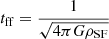 is the free fall time. The probability of forming a star particle each time step is then given by
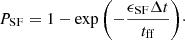
Here Δt is the length of the current timestep. When a star particle forms, it replaces the whole gas particle, this means that every star formation event will leave holes in the magnetic field. This can be seen as the magnetic flux getting trapped within the star particle. However, this does affect both the local magnetic energy and the local divergence error. Star particles that form within the simulation represent a stellar population that evolves according to stellar theory, with an initial mass function following Chabrier (2003). Feedback from stellar winds, Type Ia and Type II SNe eject mass and metals into the ISM, which reduces the mass of the star particle and increases the mass of the surrounding gas particles. If left unchecked, this can lead to situations where gas particles have significantly different masses. This is undesirable as the accuracy of the SPH method can quickly be degraded if there is a significant difference in particle masses within the smoothing kernel. A simple way to avoid this is to split the gas particles if they exceed 2 times their initial mass into two equal-mass particles with the same properties, which are placed randomly within the original particles smoothing radius. This is the default way to handle it in GASOLINE2 but can lead to more grid noise and divergence errors for the magnetic field. To reduce this error, we instead present a new particle-splitting method. The main issue with distributing the child particles within the smoothing kernel is that neighbors strongly feel the change of the particle split. In addition, because the distribution is random it can place the child particles close to other neighboring particles or across density gradients, leading to spurious fluctuations in the local field. These effects can be mitigated by instead splitting the particle within the interparticle distance (hint) instead. This is similar to the methods presented in Martel et al. (2006; particles placed on vertices of a cube with cube length  ) and Chiaki & Yoshida (2015; particles placed within local Voronoi cell). In our prescription, the two daughter particles are distributed
  away from the parent particle on a line that is orthogonal to the closest neighbor (located hint away). Making the two new daughter particles to be an equal distance away from the closest neighbor minimizes the effect of the split. When a particle now splits, the neighbors do not directly see any significant change as the position of the child particles is very close to the position of the parent particle.
All our galaxy simulations are run until the magnetic field growth has stabilized, usually around tend = 1 − 3 Gyr. The resolution, SN feedback parameters, Jeans floor, and the magnetic field configuration are varied in different runs. Below we outline more details about the parameters altered.
2.3. Jeans floor
To avoid numerical fragmentation, it is important to ensure that gas does not collapse beyond the resolvable Jeans length (Truelove et al. 1997; Bate & Burkert 1997). This can happen in galaxy simulations when the gas becomes cold and dense enough, such that its Jeans length is smaller than the resolution length of the simulation. To ensure this, we added a nonthermal pressure floor to our simulation, based on the method described in Robertson & Kravtsov (2008):
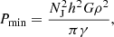
where h is the smoothing length, ρ is the gas density, and γ = 5/3 is the adiabatic index. This ensures that the Jeans length is resolved by NJ smoothing lengths. The classic condition of Truelove et al. (1997) states that the Jeans length should be resolved by at least 4 resolution lengths. However, the value required depends on several factors, such as numerical method, resolution, initial conditions, and included physics, as there can be many factors that prevent the gas from entering a phase where it’s vulnerable to artificial fragmentation. The Jeans floor effectively sets the smallest collapsed length scale in the simulation. The smallest collapsed length scale will thus be roughly Lcoll = ϵNJ. When we go to higher resolution we decrease this length scale to keep the same 4 resolution length condition as before. This, of course, is generally a desirable trait as we go closer to resolving the real deal, however for comparison sake this can muddy the result. Keeping the smallest collapsed length scale the same as we increase the resolution ensures that the turbulent injection scales remain similar. In turn, this increases the number of resolutions elements that resolves the minimum Jeans length. This can be done by introducing a scaling law (Smith et al. 2018),

Here, the subscript low represent the values given for the “Low” resolution simulation (see Table 1). As we increase the resolution by splitting all the particles by 8, the effective NJ for each higher resolution simulation becomes NJ, medium = 2NJ, low and NJ, high = 4NJ, low. While NJ = 4 is the classical condition for avoiding artificial fragmentation, the magnetic dynamo from gravitational collapse give more stringent constraints. As mentioned briefly in the introduction, Federrath et al. (2011b) found that resolving the Jeans length with at least 30 resolution elements is required to properly capture the solenoidal-compressible ratio during gravitational collapse. However, the Jeans floor simply sets the minimum local Jeans length to be resolved by NJ, the majority of scales within the simulation can fulfill the magnetic dynamo condition even if the smallest scale does not (NJ < 30). Nevertheless, the compressible modes generated at the small scales can potentially act destructively on the magnetic field growth at those scales. Therefore, it is instructive to investigate a wide range of NJ values for galaxy simulations to see its effect.
2.4. Feedback models
To investigate the effect of SN feedback on the amplification of the magnetic field in galaxies, we run several simulations with varying feedback parameters. The first parameter that we vary in our simulation is the energy injected to the surrounding ISM ESN in SN events. The three strengths that we use in our simulations are ϵSN = 1051 ergs, ESN, low = 0.5ϵSN, ESN, high = 2.0ϵSN. We also employ two different feedback models in our simulations, the blastwave model (Stinson et al. 2006) and the superbubble model (Keller et al. 2014). To experiment with different mass-loading and coupling parameters of the feedback, we vary the number of surrounding particles injected with energy during a feedback event in the superbubble model (NFB = 1, 64, 200). NFB = 1 represents the physical model of superbubble, higher values make the model unphysical as it will overshoot the expected mass-loading and limit evaporation. But we use this as an numerical experiment to alter the mass loading, as the main point of this paper is to investigate numerical effects on the amplification process.
A wide range of different feedback models have been developed to tackle the lack of resolution in galaxy simulations to resolve the Sedov–Taylor phase of a SN explosion. Early SN feedback models simply relied on a direct thermal injection to the surrounding medium. The issue with this is that the thermal energy is quickly radiated away before it can do any work on the surrounding medium as should be the case for the resolved Sedov–Taylor phase (Katz 1992). A way to combat this involves switching off the radiative cooling of gas that has received feedback energy, enforcing an adiabatic phase, for some length of time. This is the philosophy of the first feedback model we employ, the blastwave model/delayed cooling model (Stinson et al. 2006).
However, the blastwave model does have some significant downfalls. First, star formation is clustered; new stars are spatially and temporally correlated, and feedback from their individual winds and SNe merge, thermalize and grow as a superbubble rather than a series of isolated SNe. Second, because superbubbles have both hot gas > 106 K and sharp temperature gradients, thermal conduction is significant which evaporate cold gas Weaver et al. (1977; the evaporation can however be reduced when cooling on the conducting surface is included, see e.g., El-Badry et al. 2019). The superbubble feedback model from Keller et al. (2014) represents a more realistic model when simulating SN feedback from cluster of stars (which each star particle represent). This is done by introducing a separate cold and hot phase for each particle. The evolution of the superbubble is accurately captured with the help of thermal conduction and subgrid evaporation, which regulates the hot and cold phases without the need of a free parameter. This makes the model more insensitive to numerical resolution compared to the blastwave model described before. We note that, in more recent works with sufficiently high resolution (mgas ∼ 10 M⊙ or less), simulations start to resolve the Sedov-Taylor phase of individual SNe and thus no longer need subgrid models (Hu et al. 2016; Smith et al. 2018, 2021; Hu 2019; Steinwandel et al. 2020; Lahén et al. 2020; Gutcke et al. 2021; Hislop et al. 2022). While one would expect that the injection length in such models may be smaller than simulations with subgrid schemes, it has been shown in these work that star formation and SNe occurs in clusters (which is in fact a key component to drive galactic outflows), and thus the collective superbubble injection length may still be quite large. On the other hand, increasing resolution has significant impact on fluid parameters and thus the dynamo processes, which complicates the issue further. We defer a more detailed investigation on this to a future paper.
In this paper we do not employ any magnetic field injection during feedback events. This is because it is highly nontrivial how to properly inject a magnetic field into the surrounding particle distribution. We leave this to be the topic of future work.
2.5. Numerical diffusion
To get the Reynolds number and magnetic Reynolds number we estimate the numerical dissipation from the equivalent physical dissipation equations. This is done by recording the energy lost due to the artificial dissipation terms. From the Navier-Stokes equation we can estimate the shear viscosity with:
Here, we have assumed the fixed ratio between the bulk viscosity and the shear viscosity, which follows from the continuum limit derivation ( ) (Lodato & Price 2010). We estimate the physical resistivity from the Ohmic dissipation law:
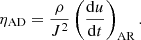
Taking the ratio of the two equations then gives us the numerical Prandtl number:

After estimating the local velocity dispersion and the injection length, the Reynolds number and magnetic Reynolds number can be estimated using Eqs. (1) and (2).
2.6. Magnetic field configuration
The strength and configuration of the initial magnetic field can play an important role in its subsequent development. The simple choice is to just apply a constant field parallel to one direction, for a galactic disk initiating it in the parallel direction of the angular momentum vector ( ) or orthogonal direction can be appropriate choices.


While not being a very realistic magnetic configuration for an evolved galaxy, it does present the system with a straightforward initial polarity which can subsequently affect the underlying field growth. The main issue with a constant field is that low-density regions can become very magnetically dominated to begin with.
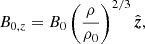
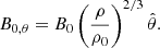
A more realistic magnetic configuration can be achieved by taking the flux freezing consideration into account, which would mean that the strength of the magnetic field would more closely follow the initial density distribution (B ∝ ρ2/3 for spherical collapse). To keep the initial magnetic field divergenceless while scaling with the density requires a more complex field configuration. The easiest way to construct such a field is with the use of a vector potential. However, the initial field will in this case be dependent on resolution and the accuracy of the gradient estimate. For the low resolution this can generate quite a noisy initial field at the free surfaces (due to noisy gradient estimates). Instead we construct a vertical and toroidal density-based field simply by:
This magnetic field will not be divergenceless to begin with, but is statically cleaned using our divergence cleaning before the proper runs. To confirm the divergenceless constraint we track the normalized divergence error initially and during the simulation
During the simulation the mean of this quantity should preferably remain below 10−2 but higher values can still be acceptable, depending on the system. We also measure the normalized Maxwell stress:
2.7. Analysis of turbulence
There are several methods by which one can go about defining the turbulent velocity. In this paper we simply remove the mean rotation from the azimuthal component:
The rotation velocity can be estimated by calculating the vcirc from the gravitational influence within the midplane or by removing the averaged cylindrical radial profile of vazi for the gas (taken over 0.15 kpc radial bins). These give similar results and we use the latter method in this paper. Another popular way to estimate the turbulence is to calculate the velocity dispersion within the smoothing kernel. However, a negative of this method is that the length scale at which the velocity dispersion is calculated will depend on the resolution and density. The effective turbulent kinetic pressure is given by:

We also define the magnetic-thermal energy density ratio ( ) and the magnetic-turbulent energy density ratio (
 ):
):


Together with the turbulent Mach number (M) and the shearing parameter (q).


Here Ω is the angular velocity and cs is the speed of sound. After the simulation the particle data is interpolated to uniform grid data for post-analysis. To analyze the scale dependencies in the simulation we perform a spectral analysis of the velocity, magnetic and density fields using Fourier analysis. The resulting Fourier energy spectra is calculated using the spherical shell method from (e.g. Frisch 1995):
Here  and
and  represents the Fourier transform and its conjugate of quantity A. The integration occurs over spherical shells in Fourier space with radius
  .
.
The compressive and solenoidal component of a given field (A) can be extracted using Helmholtz decomposition. Here, the Fourier transform is decomposed into an longitudunal and transverse component ( ). The compressible part can be found by calculating:
  and then performing an inverse Fourier transform. This gives us Acomp which can be removed from A to give the estimated solenoidal component Asol. This is then used to estimate the Fourier energy spectra for the solenoidal and compressive modes using Eq. (20). An interesting quantity to measure is the relative solenoidal to compresssive ratio at different scales.
In general, the pure velocity and magnetic energy scaling are investigated, where A = vturb and  . However, for the supersonic turbulence and the large range of scales that we cover in these simulations, it becomes more interesting to investigate the scaling dependencies of the velocity and magnetic densities, where
  and
and  5.
5.
3. Simulation results
The default initial magnetic field is set in to be in the vertical direction using Eq. (10) with B0 = 10−3 μG and ρ0 = 6.77331 × 10⁻²³, this correlates to an initial central thermal plasma beta of β0, center = 107. The artificial resistivity coefficient is set to αB = 0.5 as the code default. For the simulations including feedback the default is the superbubble scheme with strength 1ϵSN and number of injection particles set to NFB = 64.
3.1. Simulations with no feedback
In an attempt to discern the subsequent dynamo effects induced by different subgrid physics, we have performed several simulations without feedback and star formation. These simulations still include radiative cooling and a Jeans floor. This removes one of the main contributors (feedback) of turbulence and vertical motions from the simulation, leaving the gravitational collapse and shear as the determinant factors. The underlying kinematics will thus be highly dependent on the cooling and the given Jeans floor (setting the minimum collapse length). We perform two sets of simulations using the initial vertical and toroidal magnetic fields of Eqs. (8) and (9), and with varying Jeans floor (NJ = 4, 8, 10, 16) to investigate how the magnetic field amplifies in different conditions. The simulations are run up to varying times depending on the saturation conditions of the magnetic field. The results of the simulations are shown in Figs. 1–7.
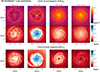 |
Fig. 1. Face-on evolution of the no feedback simulations with varying Jeans floor and initial magnetic field geometry (B0, z two top panels, B0, ϕ bottom panel). The time for each column/Jeans floor (NJ = 4, 8, 10, 16) is t = (0.5, 1, 1, 1) Gyr respectively. The NJ = 8 case exhibits the strongest magnetic field growth at early times, likely through an active GI or αΩ dynamo within the developed filamentary structure. Further reducing the Jeans floor leads to too much fragmentation of the disk, reducing the effect of the active dynamo. For higher Jeans floor GI remain quite weak at this time, leading to either a weak amplification or decay of the magnetic field in the disk. However, in the case of the NJ = 10 and Bz, 0 where a small fragment has started to form, the disk will become unstable at a later time (see Fig. 6). |
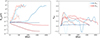 |
Fig. 2. Time evolution of the average magnetic field strength (left panel) and the normalized Maxwell stress (right panel) for the no feedback runs. Blue lines represent simulations with an initial vertical field and the red lines represent simulations with an initial toroidal field. Darker colors represent higher Jeans floor (NJ = (4, 8, 10, 16)). The NJ = 4 and NJ = 8 simulations have a rapid amplification in the magnetic field early on due to spiral arm compression. We can see that we get the strongest αMW exhibited during the growth phase of the NJ = 8 cases, correlating to the generation of radial and toroidal fields during the dynamo process. The elevated level in αMW for all the cases with an initial toroidal field is simply due to the initial field and normalization (Bz ≈ 0). |
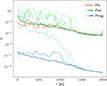 |
Fig. 3. Radial profiles of the magnetic, turbulent and thermal pressures for the no feedback runs at around t = 1 Gyr. Darker colors represents higher Jeans floor (NJ = (4, 8, 10, 16)). For the thermal pressure we only plot one line as it is similar across these simulations. For the NJ = 8 case we can see that the magnetic pressure is of similar strength as the thermal pressure in the center of the disk. The magnetic pressure decreases with radius and returns to initial values beyond 14 kpc. The turbulent pressure can be seen to significantly increases in both NJ = 4 and 8 as the disk is highly gravitationally unstable. |
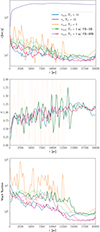 |
Fig. 4. Radial profile of the velocity (top), the shear parameter (middle) and the Mach number (bottom) for the NJ = 8 and NJ = 16 no-feedback runs and for the SB and BW feedback runs with NJ = 8 (light color t = 250 Myr, dark color 2 Gyr). The turbulent velocities are enhanced by the gravitational instability of the disk and the inclusion of feedback. However, BW can be seen to produce a lower turbulent response compared to SB, especially at later times (within 10 kpc). In all runs we can see that there is a reduction of the shearing parameter toward the central region, reducing the effectiveness of an αΩ type dynamo. Mach numbers are lower in the BW model due to the heating of the disk and the relatively low turbulent velocities. |
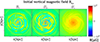 |
Fig. 5. Magnetic field polarity of the NJ = 16 no feedback simulation at t = 1 Gyr with an initial vertical field. We can see field reversals throughout the disk in both the radial and toroidal directions. These are highly correlated to the spiral arm structure, as the reversals form together with the velocity perturbation induced by spiral shocks (Dobbs et al. 2016). The vertical field remains fairly correlated to the density and is similar in strength to the initial setup. |
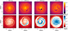 |
Fig. 6. Development of a fragment within the disk for the NJ = 10 B0, z case at later times (t = 800 − 2000 Myr), which subsequently destabilizes the disk and generates a strong magnetic field in the process. Top panel shows the density rendering and the bottom panel the magnetic field strength. |
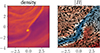 |
Fig. 7. Closer look at the magnetic field structure around the fragment at t = 1300 Myr. It is clear that the magnetic field traces the filamentary structure, with opposite/unstructured magnetic fields occurring in the low-density region around it. This is similar to the magnetic field structure formed from the GI-dynamo simulations of Riols & Latter (2019), which due to magnetic flux redistribution generates opposite radial mean fields within and outside the spiral arm. In addition, we can see that there is a strong field reversal in the gap in front of the fragment. |
In Fig. 1 we can see the state of the galactic disk of our different runs at around the same time. We can see that we get very different amplification and behavior when changing the Jeans floor. Lower Jeans floor allows for more collapse of the gas and stronger spiral arm dynamics within the disk, which seems to greatly increase the amplification of the magnetic field within the disk. There is, however, not a linear dependence on the magnetic field amplification and lower Jeans floor. The NJ = 4 case initially experiences a quick amplification of the magnetic field within the collapsing spiral arms. However, this amplification is eventually damped as the spiral arms fragment and lose interconnectivity. If we compare this to the NJ = 8 case we can see that while the spiral arms in this case also fragment, there exists more elongated spiral arms and higher connectivity between the fragments. Amplification in this case occurs rapidly, reaching a saturated state after around 500 Myr (Fig. 2). The radial profile of the magnetic, turbulent and thermal energy densities (Fig. 3) reveals that the magnetic field reaches equipartition in the center of the disk, which strength then tapers off as we go to larger radius. Looking at the evolution of the averaged Brms within the disk, we can see that it is quickly amplified to about 10 μG, where it eventually saturates. From Fig. 2 we can see that during the amplification stage the average αMW peaks within the disk. During the evolution of the galaxy, we observe plenty of field reversals within and around the spiral arms, where the main amplification takes place, indicating that we have an active dynamo cycle acting in this region. These spiral arms strongly interact with each other as they move radially through the disk. This can lead to strong magnetic field amplification, as the spiral arms gets entangled. In addition, the spiral arms oscillate in the vertical direction (around 100 pc), which increases the entanglement of the spiral arms as they interact, which can lead to further magnetic field amplification.
As we increase the Jeans floor even further (NJ = 10 and NJ = 16), we can see that we have less collapse, and at the time of Fig. 1 there is no significant fragmentation of the disk. In NJ = 16 the spiral compression is highly reduced, which dampens the magnetic field amplification. The amplification from shear and small turbulent motions in the disk solely remain to balance out the dissipation/diffusion of the magnetic field. In the high Jeans floor cases an apparent difference between the initial magnetic field orientation arises. From Fig. 1, we can see that in the case of a toroidal field the center region becomes highly damped. Furthermore, in the case of NJ = 16 there is dissipation throughout the whole disk. The dampening of the central region in the toroidal cases can also be seen at early times for NJ = 8 before significant amplification has occurred. We believe that the main reason for this is that particles whose smoothing kernel crosses the central axis of the disk will “see” a very discontinuous magnetic field in the case of an initial toroidal field and the artificial resistivity will attempt to smooth it out leading to high dissipation of the field in this region. This will not be the case with an initial vertical field as it will vary smoothly across the axis. In addition, for both cases the central region will have a significantly reduced ability to amplify the magnetic fields compared to the outer regions due to a lower shearing parameter (see Fig. 4). As we mentioned previously, amplification in these high Jeans floor cases will be driven strongly by shear and the vertical motions of the turbulence. Apart from the numerical resistivity, there is additionally also turbulent diffusion and advection of the mean magnetic field that can affect the amplification. Divergence cleaning might at first also seem like a probable cause for the dampening within the center region, however, we have tested without divergence cleaning and the dampening still remains.
Looking at the polarity of the NJ = 16, B0, z disk in Fig. 5, we can see that we have magnetic field reversals in both the developed radial and toroidal field structure. These field reversals primarily form in the inter-arm regions, and have been shown to be associated with the velocity changes across the spiral shocks that form within the disk (Dobbs et al. 2016). The vertical field remains similar to the initial field structure, with the magnetic field strength continuing to be highly correlated to the density.
An interesting feature can be seen in the case of NJ = 10 for an initial vertical field, at around x = −6, y = −6 in Fig. 1, where a fragment has started to develop. Running this simulation for longer, we can see from the time lapse in Fig. 6, that this fragment together with its connecting filaments causes an instability to occur in the disk, leading to a subsequent rapid amplification of the magnetic field, similar to what was seen in the NJ = 8 case. Looking at the magnetic field generated around the fragment in Fig. 7, we can see that it is highly entwined with the connecting high dense filamentary structure, stretching the field toward the radial direction. In the low-density region in front of the fragment we can see that the field reverses its direction. As time goes on, the fragment and filaments move radially inward as can be seen in Fig. 6. In addition, the fragment oscillates in the vertical direction around the central plane. Strong magnetic fields can be seen to be generated in the wake of the fragment as it sweeps up gas.
Strong candidates of the dynamo action induced in the spiral arms in these simulations is an αΩ type dynamo, where radial fields are induced by either large-scale motions as in the GI-dynamo or turbulent motions as in the classic αΩ dynamo. In the GI-dynamo we expect large-scale vertical rolls to be generated above the disk. While there is significant vorticity within the velocity field above the disk, clear vertical rolls cannot be seen and the velocity field looks highly turbulent. The strongest amplification can be seen in the filamentary structures that move inward in the disk and has magnetic fields that are strongly dragged along the radial direction. This can partly be understood by considering the terms governing the generation of radial fields within mean-field dynamo theory. The electromotive force (EMF) involved in generating the radial fields has two main components, the part that originates from vertical motions ( ) and the part that originates from radial motions (
 ). Radial fields generated through the pinching of the field lines within the filaments are lifted by vertical motions (either turbulent or large-scale) that redistributes the radial fields in the vertical direction, leading to a segregation of the magnetic flux, giving an opposite positive/negative mean-field within the filament and in the corona. These vertical motions can in addition induce vertical magnetic fields bz that together with radial motions ur can stretch and fold the field lines in the radial direction. The collective effect of these two components will depend on how net-correlated the magnetic field and velocities are. The effect seen here replicates many of the features seen by the GI-dynamo as described by Riols & Latter (2019), where radial flux redistribution within the spiral arm was found to generate opposite mean radial magnetic fields within the spiral arm and its surroundings (corona and interarm region). This is similar to the phenomena that we witness in Fig. 7, where the magnetic field can be seen to be highly connected to the filamentary structure, with opposite/unstructured magnetic fields occurring in the low-density region around it. We can in addition see that fluctuating vertical fields are increased within the filament region. The small vertical bulk motions of the filament and fragment might add extra complexity to the dynamo processes as the vertical density structure around it will become more asymmetric as it moves away from the central plane. In the case of NJ = 8 there is also significant interaction between the spiral arms that likely boost the amplification of the dynamo. A full mean-field analysis is required to separate the effective scales and the contribution of each component. This would allow one to more easily distinguish between the GI-dynamo and the classic αΩ dynamo in this case. This is beyond the scope of this paper and we leave it to be explored in future work.
3.2. Simulations with feedback
3.2.1. The early amplification phase and its dependence on resolution
In the following sections we look at the effect of adding star formation and feedback to our simulations. In this section we investigate the early amplification phase of the magnetic field and its dependence on resolution. To reduce the computational cost of our highest resolution simulation, NFB = 1 is used for the simulations in this section. Apart from this, the initial configuration as outlined in the beginning of Sect. 3 is used. We run three simulations at different resolutions (Table 1), which we refer to as the “Low”, “Medium” and “High” simulations. The Jeans floor adjustment is taken into account to resolve the same collapse-scale across all resolutions. This correspond to resolving the Jeans length by NJ = 4, 8, 16 for the Low, Medium and High simulations, respectively. The Low and Medium simulations are run for around 2 Gyr, while the High simulation is only run for 250 Myr due to being computationally demanding. The results of the simulations are shown in Figs. 8–12.
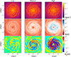 |
Fig. 8. Face-on rendering of the galactic disk after t = 250 Myr. Comparing the effect of resolution on the early evolution of the galaxy. Left to right goes from low to high resolution. Top panel show density, middle panel magnetic field strength and the bottom panel the toroidal magnetic field. We can see that the scale of the developed mean fields are about the same but increases in strength with resolution. |
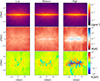 |
Fig. 9. Side-on rendering of the galactic disk after t = 250 Myr. Comparing the effect of resolution on the early evolution of the galaxy. Left to right goes from low to high resolution Top panel show density, middle panel magnetic field strength and bottom panel the toroidal magnetic field. The increase in resolution show additional the CGM. Feedback leads to the formation of an interesting vertical structure of the magnetic field, where near the central disk, we can see plenty of reversals and intricate behaviors in the magnetic field. The complexity of the structure around the central disk increases as we increase the resolution. The outer regions can be seen to be dominated by the blowout of the initial magnetic flux. |
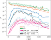 |
Fig. 10. Radial profiles of the magnetic, turbulent, and thermal pressures for the resolution study at a few different times (with later times being represented by the given color palette getting darker). For the low-resolution simulations, we did not see any significant amplification as time went by. Whereas for the medium-resolution ones, we reached a saturated state after about 1.4 Gyr. The high-resolution simulations reached a similar magnetic field strength to the medium resolution at 800 Myr after just 250 Myr. |
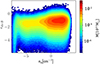 |
Fig. 11. Mass-weighted phase diagram of the divergence error(ϵdiv, B) for the high-resolution simulation at 250 Myr. The mean divergence error is between ϵdiv, B ≈ 10−1 − 10−2. |
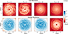 |
Fig. 12. Face-on rendering of the magnetic field strength of galactic disk after t = 2.0 Gyr. Simulations with feedback, comparing the effect of different Jeans floor on the evolution. Top panel show the Low resolution simulation and bottom the medium resolution. We can see that we get no significant amplification in the low resolution, while strong amplification is seen in the medium resolution. Too high Jeans floor diminishes the dynamo processes as the smallest collapse length becomes too large. |
In Figs. 8 and 9, we can see the state of the galactic disk of our resolution study after around 250 Myr. It is clear that we have a strong resolution dependence on the amplification of the magnetic field. Due to the cold initial conditions, there is a starburst in the beginning of the simulation. This leads to strong initial outflows that advects the magnetic field outward and a temporary decrease in the magnetic field within the disk. But the magnetic fields are quickly strengthen by the dynamo processes active in the disk. The amplification of the magnetic field can be seen to mainly occur in the spiral arm region of the disk, whereas in the center of the disk there is no/much less amplification. This is highlighted in Fig. 10, which shows the radial profile of the turbulent, thermal and magnetic pressure. It is clear that the shape of the magnetic pressure curve is similar across all the simulation, indicating a similar amplification process across all the simulations. This is further seen in the scale of the toroidal mean fields generated within the disk (bottom panel in Fig. 8), which polarity remain at a similar scale across the three resolutions. While all three resolutions exhibit a similar mean-field dynamo, there is a clear resolution dependence on the effective growth.
In Fig. 10 we have additionally plotted the radial profiles of the magnetic pressure at later times for the Low and Medium resolution simulations. The Medium resolution subsequently amplifies and reaches a saturated state of around 10% of equipartition with the thermal energy, which occurs at around 1200 Myr. The Low resolution, on the other hand, do not exhibit any significant amplification and roughly keeps the strength of the initial magnetic field (averaged over the disk). At the same time, we can see that the High resolution simulation has already amplified the magnetic field at t = 250 Myr to similar strengths as the Medium resolution simulation at t = 800 Myr. While the radial pressure shape of the Low, Medium and High is similar, there are some interesting differences. The Medium and High simulations that amplify the magnetic field have a peak of around 4−6 kpc, with a fairly constant plasma beta ratio between the thermal and turbulent velocity between 4−15 kpc. For the High resolution simulation we can see that we have a stronger drop off at 12 kpc. This is likely due to the simulation being at a much earlier time (t = 250 Myr) than the comparative Medium resolution curve (t = 800 Myr), which indicates that 4−12 kpc is the region with the highest amplification, correlating to the region which exhibit most feedback bubbles and spiral arms. As time goes on, the magnetic field can be seen to be amplified in the outer and central regions of the disk, through both the advection and diffusion of the strong field regions and potentially through a slower dynamo amplification process in these regions. Feedback also leads to the formation of an interesting vertical structure of the magnetic field, where near the central disk, we can see plenty of reversals and intricate behaviors in the magnetic field (see bottom row in Fig. 9). Further out from the disk we can see that the magnetic field is mainly dominated by the initial vertical flux that is blown out early on in the simulation. Additional structure can be seen to emerge in this low-density region as we increase the resolution.
Due to the formation of large-scale mean fields, it is likely that we have a mean-field dynamo acting in these simulations. Small-scale dynamo can of course also be active within these simulations, but would not be able to generate the observed mean fields. We discuss the potential and effectiveness of small-scale dynamo in these simulations further in Sect. 3.2.4. While both these runs and the no-feedback runs appear to amplify due to a sort of αΩ-dynamo, there are some difference between the effective amplification processes. This can clearly be seen in the developed radial profile of the magnetic pressure in Figs. 3 and 10. In the no-feedback run the magnetic field strength becomes concentrated in the center of the disk as the fragments move radially inward through the disk. While in the feedback runs the magnetic strength is concentrated outside the central region, keeping a similar ratio between the thermal and magnetic pressure in the range 4 − 16 kpc.
The major difference lies in the expansion of the vertical scale-height of the galaxy as we introduce feedback. This causes an increase in magnetic flux transfer from the central disk region to the CGM and an overall increase in the simulated system volume. This increases the magnetic strength in the CGM, but can do so at the expense of the magnetic field within the central disk. On the other hand, the increased vertical motions induced by feedback acts to increase the effectiveness of αΩ type dynamos. The increase in resolution allows for more small-scale structure in the CGM and seem to correlate to a more effective mean-field dynamo in the disk. It is reasonable that this increase in small-scale structure further increase the effectiveness of the dynamo, as it would lead to more resolved flow structure (for example the vertical rolls in the GI-dynamo). From Fig. 4, we can also see that the superbubble feedback in general increases the turbulence in the disk and leads to a higher mach number within the disk. This can have both a positive and destructive effect on the growth of magnetic fields. Increased turbulence will have a positive effect on both small-scale and mean-field dynamo processes as it is the main driver. For the small-scale dynamo, the increase in turbulence mainly has a positive effect on the growth rates given that the fluid parameters (Re, Remag, Pm) are high enough. For the mean-field dynamo, the turbulence act to increase the vertical and radial motions, which benefit the amplification. However, for the mean-field, turbulence can also act in a destructive fashion, by increasing the turbulent diffusion within the disk and increasing the ejection of magnetic flux from the central plane. The dampening of the central region likely occurs due to the destructive effects being dominant in this region.
In Fig. 11 we have plotted the mass-weighted phase diagram of the divergence error which shows that the divergence errors are comparable or better than previous Lagrangian codes, which usually lie in the range ϵdiv, B = 10−1 ↔ 101 (Kotarba et al. 2009; Pakmor & Springel 2013; Dobbs et al. 2016; Steinwandel et al. 2019). We further discuss the effect of resolution in the following sections but with the addition of changing other parameters.
3.2.2. Effect of Jeans floor
This section aims to investigate the effect of altering the numerical Jeans floor of our feedback simulations. This is similar to the investigation done in Sect. 3.1 for our no-feedback runs. We vary the Jeans floor between (NJ = 4, 8, 16, 30) and run two sets of simulations at Low and Medium resolution (see Table 1). For everything else the default initial values are used (Sect. 3) and the simulations are run to around t = 2 Gyr. The results of the simulations are shown in Figs. 12–15.
In Fig. 12 we can see a rendering of the magnetic field strength in the galactic disk between all our runs at t = 2 Gyr. The most stark difference seen is the effect of resolution, where 1 − 30 μG develop in the Medium resolution while barely any amplification occurs in the Low resolution. This is similar to what we observed in the previous section when we looked at resolution dependence. Similar to the no-feedback runs, we can see that the galactic disk experience much less dynamics when the collapse length is too large, above NJ = 16 for the Low resolution and above NJ = 30 for the Medium resolution. Below these NJ values we can see that the magnetic field saturates to a similar value across the simulations independent of the Jeans floor. This is further highlighted in Fig. 13 where we have plotted the radial profile of the energy density ratios for the saturated Medium simulations (NJ = 4, 8, 16). In between 4 and 15 kpc, we can see that all the runs saturate at around 10 − 30% of the thermal pressure, while reaching only around 5% of the turbulent pressure. We can see that the NJ = 8 reaches higher saturation in the inner region 2 − 4 kpc compared to the other cases. It is interesting that if one compares these runs to the physical superbubble model (NFB = 1) Medium run from the previous section, the increase in the number of feedback particles in these simulations produces a significant increase in the saturation strength beyond 10 kpc (as seen in Fig. 13). However, this is mainly due to the NFB = 1, having hotter winds and resulting higher thermal energy in the outskirts. The main dependence on the Jeans floor seem to arise when we look at the time evolution between these different runs. As can be seen from Fig. 14, there is a positive correlation between the growth rate of the magnetic field and the Jeans floor, given that the collapse length is sufficiently small. Saturation is achieved at around t = 1000 Myr for NJ = 16, t = 1100 Myr for NJ = 8 and t = 1300 Myr for NJ = 4. From this it also becomes apparent that the NJ = 30 run experiences a growth phase in the magnetic field to about t = 800 Myr, while then starting to slowly decay. Due to the initial cold state, there is some feedback occurring early in its evolution which increases the dynamics of the galaxy and induces magnetic amplification. However, when the star formation slows down and the galaxy calms down, the magnetic field starts to slowly decay. Compared to the no-feedback runs, we can see that the normalized Maxwell stress remains around αMW ≈ 0.2 for NJ = 4, 8, 16 and there is no significant increase during the growth phase (Fig. 14). For NJ = 30 there is however, an increase in normalized stress during the growth phase αMW ≈ 0.4, which reduces to around αMW ≈ 0.2 as it starts to decay. Another effect that we can see from these simulations are that the divergence error becomes smaller for larger Jeans floor. In Fig. 15, we can clearly see that the divergence error within the disk is reduced as we increase the Jeans floor from NJ = 8 to NJ = 16. This is likely due to the fact that we have more smooth collapsed structures within the disk, which has better resolved gradients that in turn causes less divergence errors to be produced.
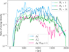 |
Fig. 13. Radial profile of the energy density ratio (β−1) for the saturated medium resolution runs in Fig. 12. We have included lines for both the magnetic-thermal energy density ratio ( |


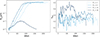 |
Fig. 14. Time plots for the medium resolution feedback runs with varying Jeans floor. The left and right panel shows the evolution of Brms and αMW respectively. Darker colors represents higher Jeans floor. We can see that there is a positive dependence on the Jeans floor for the amplification rate, as long as a “critical” collapse length is resolved. The normalized Maxwell stress lie around αMW = 0.1 − 0.3 for all runs. There is additional stress within the NJ = 30 simulation during the early amplification phase with around αMW = 0.4. |
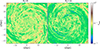 |
Fig. 15. Face-on rendering of the divergence error of the magnetic field in the galactic disk after t = 2 Gyr. We can clearly see that there is a reduction in divergence error throughout the disk for higher Jeans floor. The mean divergence error in the NJ = 8 is around ϵdiv, B = 10−1 and in the NJ = 16 around ϵdiv, B = 6 × 10⁻². |
3.2.3. Effect of feedback
From the previous sections, we have seen that the inclusion of feedback significantly alters the galactic dynamo. Feedback boosts dynamo action in the spiral arms through the injection of vertical fountain motions, but at the same time it can lead to a decrease in magnetic field strength through the dissipation and advection of magnetic flux from the central region. In this section we look at the difference between the blastwave (BW) and the superbubble (SB) feedback models. We also look at the effect of varying the feedback strength (ϵFB = 0.5ϵSN, 1ϵSN, 2ϵSN), and for the SB model, we vary the number of neighbors we inject the feedback into (NFB = 1, 64, 200). We reiterate that NFB = 1 represents the physical model of superbubble and that higher values make the model unphysical as it will overshoot the expected mass-loading and limit evaporation (Keller et al. 2014). However, increasing the injection length of the SB model will change the mass loading and the resulting turbulence within the disk, which is an interesting parameter to investigate in terms of the galactic dynamo. We run both Low and a Medium resolution simulations. The simulations are run to around 2 Gyr and the results are shown in Figs. 16–18.
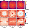 |
Fig. 16. Rendering of density, magnetic field strength of the Low resolution simulations with varying feedback scheme at t = 2 Gyr. Strong field growth can be seen for both the blastwave model and the high coupling superbubble model (NFB = 200). Both the blastwave model and the physical superbubble model (NFB = 1) leads to small feedback bubbles which pushes material far away from the disk. The mass loading in the superbubble model (NFB = 1) is however much larger as the blastwave model mainly generate hot low-density outflows, this means that there is less transfer of magnetic fields from the central region in the blastwave model. Increasing the injection length (NFB = 200) leads to more mass loading, larger feedback bubbles and a more concentrated vertical structure, which in turn lead to more amplification of the magnetic field within the central disk. |
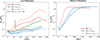 |
Fig. 17. Time evolution of Brms within the central disk for different feedback schemes. Left panel show the Low resolution runs and right panel show the Medium resolution runs. Darker colors in blue and red indicate stronger feedback strength and light green represent the physical SB model (NFB = 1) and dark green represent SB model with higher coupling (NFB = 200). Its clear from both resolutions that the blastwave scheme produce faster amplification than the superbubble schemes. Higher energy injection does in general lead to slower growth of the magnetic field within the central disk. Increasing the coupling/injection length of the superbubble scheme does seem to generally have a positive effect on the magnetic field amplification. The bump seen in the NFB = 200 evolution is due to rapid amplification of the magnetic field during the merger of two fragments within the central region, which afterwards is quickly dispersed outward from the central disk. |
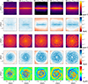 |
Fig. 18. Rendering of density, magnetic field strength and toroidal magnetic field of the medium resolution simulations with varying feedback schemes. The blastwave model generates hotter winds and less mass loading than the superbubble model, leading to less magnetic field advection from the central plane of the disk. This generates a more radial compact structure for the magnetic field. Increasing the injection length in superbubble makes the vertical density structure more compact, leading to more resolved vertical velocity structures. In addition, we see a clear increase in the scale of the toroidal mean-field with the feedback strength as the galaxy extends both radially and vertically. |
We first take a look at the effect of the two feedback models. In Fig. 16, we can see result from the Low resolution runs. It is clear that we have stronger magnetic field growth within the inner regions of the BW simulation. Looking at the density structure we can see that BW produces smaller feedback bubbles and a more smooth central region than the SB feedback. In the same figure, the effect of feedback injection can be seen, where there is a positive correlation to the amplification with increasing injection particles (higher coupling to gas). The density structure shows a more large-scale spiral structure with a larger feedback bubble appearing. Within the BW model and the physical superbubble model (NFB = 1), the magnetic field is advected outward to a larger radius, while in the high coupling superbubble model (NFB = 200) we see a more concentrated vertical magnetic field structure. Due to the BW model producing stronger magnetic fields in the disk than the physical superbubble model (NFB = 1), we see stronger magnetic fields being advected to the CGM.
The time evolution of the central disk of all the Low resolution runs can be seen in the left panel of Fig. 17. For the BW model, we can see that as we increase the feedback energy, we get less magnetic field amplification within the disk. For the SB model the amplification is independent of the feedback strength and the only case that see significant amplification is the simulation with high coupling (NFB = 200). There is an interesting spike in the magnetic field strength for the NFB = 200 simulation early in its evolution. This is caused by the merger of two fragments within the central region of the disk. Significant amplification occurs within the shear layer between the two fragments during inspiral. The amplified magnetic field within the shear layer is subsequently diffused throughout the bulk and envelope of the two fragments. This is similar to what have been seen in high-resolution simulations of binary neutron star mergers (Palenzuela et al. 2022). After the merger the produced magnetic fields are quickly diffused and advected away from the central region of the disk. This can be seen to occur in both the radial and the vertical directions, leading to a reduction in the mean magnetic field strength of the central disk.
Looking at the right panel of Fig. 17 we can see the time evolution of the Medium resolution runs. Here we can see that all runs are amplified significantly and saturate on the order of B = ∝1 μG. Similar to the Low resolution case, there is significant faster amplification in the case of the BW model, which reaches B = ∝1 μG in about 500 Myr6. For the high coupling SB feedback we can see that NFB = 64 with ESN = 0.5ϵSN and ESN = 1ϵSN reaches saturation at about the same time. With higher feedback strengths we can see that it takes about 1500 Myr to reach saturation within the central disk. With NFB = 1 saturation is reached after 1200 Myr and the saturation level is lower and similar to that of the BW model.
The reasons for these differences are best illustrated by taking a look at the renders of the Medium resolution runs in Fig. 18. Both the BW model and the physical SB model with NFB = 1 pushes material far away from the disk in the vertical direction, this allows for the advection of magnetic fields far from the disk. However, from the density rendering it appears that the SB model distributes gas closer to the disk than the BW model7. This is consistent with previous studies, which found that the SB model generally produce slower winds, but with higher mass loading factor (Keller et al. 2015; Mina et al. 2021). This implies that the turbulence generated within the ISM of the BW model is efficient in driving the dynamo but remains not too disruptive to dampen the field. In comparison, the physical SB model with NFB = 1 disturbs the ISM more, leading to less amplification. The quick amplification in the BW model is likely further amplified by its higher star formation rate early on in the simulation, with a higher peak during the initial starburst and higher than all the SB models until around 350 Myr. At the end of the simulation the star formation rate in the BW model is lower than the SB models. Increasing NFB from 1 to 64 essentially leads to more “gentle” galactic winds, with gas ejected being distributed closer to the disk. This increases the amount of resolved large-scale eddies in the vertical-direction, and thus we see a more effective dynamo. Within the same model, increasing the feedback strength increases both the vertical and radial extent of the disk. In the bottom panel of Fig. 18, we can see the toroidal magnetic field in the disk. From this we can see that the scale of the toroidal mean-field increases with the feedback strength. How vertically concentrated the disk structure is seem to be a strong determinant of the amplification rate within the central disk seen in Fig. 18, even though the saturation level is higher in the high coupling SB models (NFB = 64). However, the lag in amplification of the higher feedback strength models may simply be due to these models having a larger volume, where more magnetic energy has to be produced in total before saturation can be reached.
Looking at the averaged vertical profile of the galaxy8 in Fig. 19, it is clear that the energy density of the magnetic field is correlated to the turbulent energy density. The turbulent energy density of the BW model is significantly lower than the SB models close to the central disk. However, both profiles of the BW model and the physical SB model (NFB = 1) remain more flat at large distances than the ones from simulations with higher coupling (NFB = 64). This is reflected in the magnetic energy density and is related to the advection of magnetic fields from the central plane. In the BW model we can see that the thermal energy density is significantly higher than the resulting turbulent energy close to the disk. This differs from the SB model, in which they are always closely linked. In general a lower turbulent velocity and lower Mach number is seen in the BW model (see Fig. 4).
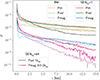 |
Fig. 19. Vertical structure of the kinetic, magnetic and thermal energy density for our medium resolution runs with varying feedback scheme around 2 Gyr. The magnetic energy density can be seen to follow the kinetic energy quite closely within the CGM. With stronger magnetic fields being present further out in the strong feedback simulations. |
It is clear from these results that the Low resolution simulations do not show the same converged behavior as the Medium resolution. This points to a failure to resolve the relevant amplification processes in the Low resolution simulations, either due to reduced dynamo efficiency or too much diffusion. In the next section we take a closer look at this.
3.2.4. Effect of diffusion parameters
Another important property in the amplification of the magnetic field comes from the diffusion parameters of the fluid: the Reynolds number, magnetic Reynolds number and the Prandtl number. In numerical simulations the two factors that determine these properties are the resolution and the numerical diffusion. The equations of the numerical estimated physical dissipation parameters are given in Sect. 2.5. In these simulations we leave the numerical viscosity alone and only vary the numerical resistivity. This is done by changing the αB parameter within the numerical scheme9. Care is however required, as a too low value can lead to excessive numerical noise/errors.
In Figs. 20 and 21, we compare four simulations, with different resolutions and different αB; two with αB = 0.25 and two with the default value of αB = 0.5. In Fig. 20 we can see that lowering the numerical resistivity enables the Low resolution simulation to grow its field much faster, leading to saturation after about 1.9 Gyr. Showing a similar resolved behavior as the Medium resolution simulations (see also Fig. 18). Faster growth is also seen in the Medium resolution (αB = 0.25), where saturation is achieved after about 700 Myr compared to 1100 Myr in the default run. In addition, the field saturates at a higher level with αB = 0.25. In Fig. 21 (early time t = 0.25 Gyr) and Fig. 22 (late time t = 2 Gyr) we can see the radial profile of the density-averaged numerical dissipation parameters. Here, we have assumed that Linj = 1 kpc and σv = vturb. The average Prandtl number can be seen to be below 1 throughout the disk, with decreasing values toward the center. Reducing the numerical resistivity can be seen to increase the Prandtl number and the magnetic Reynolds number as expected. At late times (2 Gyr) we can additionally see that the Prandtl number increases with the resolution. This might be unexpected at first glance as both dissipation schemes are of second order (∝h2), that is to say that a doubling of resolution should result in 4 times lower numerical dissipation. This can be seen to be the case for the early time (0.25 Gyr) simulations, where the Prandtl number stays roughly the same and the magnetic and regular Reynolds number increases equally in proportion to the resolution. This is because the density, velocity and magnetic field structure of the disk is more different between resolutions at later times than at early times. Another interesting behavior of the Prandtl number is its decline toward the center, as you would expect an equal or higher value in the central region. This is related to the curves of the magnetic and regular Reynolds number, where the magnetic Reynolds number has a more flat curve than the regular Reynolds number. We believe that this is related to the differences in artificial switches for the viscosity and resistivity. Artificial switches are based on local environment factors, to reduce the dissipation away from shocks. Meaning that the two schemes are not necessary correlated when the environment changes, which is what occurs when we move radially inward throughout the disk. The magnetic Reynolds number is shown here to be relatively low (Remag = 10 − 400) compared to the levels potentially required for the small-scale dynamo (Remag = 30 − 2700).
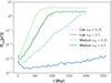 |
Fig. 20. Time evolution of Brms within the central disk for different numerical diffusion and resolutions. We can see that lowering the numerical diffusion has a clear positive effect on the growth rate and saturation level. Even the Low resolution reaches saturation in the case of αB = 0.25, after around 1.9 Gyr. |
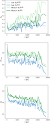 |
Fig. 21. Density-averaged radial profile of the fluid parameters for different resolutions and numerical diffusion at t = 2 Gyr. From top to bottom we have: the Prandtl number, the magnetic Reynolds number and the regular Reynolds number. The Prandtl number can be see to be below unity across the whole radial extent, with a decreasing trend toward the center. There is an expected increase due to lowering artificial resistivity and also an increase in Pm due to resolution in the outer regions of the disk (≥4 kpc). Both the magnetic and regular Reynolds number can be seen to increase toward the center; however, the magnetic Reynolds number remains flatter throughout the disk than its hydrodynamic counterpart. |
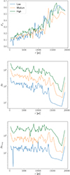 |
Fig. 22. Density-averaged radial profile of the fluid parameters for different resolutions at an early time (t = 250 Myr αB = 0.5). From top to bottom we have: the Prandtl number, the magnetic Reynolds number and the regular Reynolds number. The Prandtl number seem to be largely independent of the resolution and mainly be effected by the conditions within the galaxy (supersonic + shear + stratified environment). Both the magnetic and regular Reynolds number can be seen to increase with a factor of 4 as we increase the resolution, which is in agreement with the expected second order of the numerical diffusion. |
3.2.5. Effect of initial magnetic field strength and geometry
For our Low resolutions simulations, we also explore what the effect of the initial magnetic field strength and geometry has on the evolution of the field. The initial magnetic field strength is varied, such that the central strength is equal to a set plasma beta value. Here we set the initial central plasma beta value to roughly β0, center = (0.1, 1, 104, 107), this represents a field strength of Binit = (10, 3, 0.3, 10−3) μG at ρ = ρ0 = 6.77331 × 10⁻²³ g cm−3. We simulate with both an initial vertical field and a toroidal field following Eqs. (10) and (11). For β0, center = 104, 107 we also vary the artificial resistivity parameter αB = 0.5 and αB = 0.25.
The time evolution of the magnetic field within the central disk for these simulations is plotted in Fig. 23. For the low plasma beta runs (β0, center = 0.1, 1), we can see that the magnetic field strength is quickly reduced at the beginning of the simulation but eventually saturates around 1 μG. This is just slightly lower than the saturation levels that are achieved by the lower resistivity runs (αB = 0.25). For the high beta runs β0, center = 104, 107 we can see a similar behavior as the previous Low resolution simulations (Sects. 3.2.1–3.2.3), where the effective amplification is highly damped and the “convergence” behavior seen in the Medium and αB = 0.25 Low resolution runs is lost. There seems to be no real significant difference between starting with toroidal or vertical fields on the subsequent amplification. Looking at the right panel of Fig. 23 we can see the evolution of the vertical and toroidal mean fields. From this, we can see that the simulations with low plasma beta (β0, center = 0.1, 1) quickly lose their initial vertical/toroidal flux. In addition, we can see that the vertical flux simply reduces to noise around 0, while the toroidal flux can be seen to experience larger oscillations within the central disk.
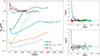 |
Fig. 23. Time evolution of Brms (left panel) and the vertical and toroidal fluxes (right panel) within the central disk for different initial field strengths and geometry. Darker lines represent a lower initial thermal plasma beta βth within the center of the disk. The distinct levels of initial central plasma beta are (β0, center = (107, 104, 1, 0.1)). We can see that for the low plasma beta cases (β0, center ≤ 1) the magnetic field strength is quickly reduced at the beginning of the simulation, but eventually saturates at a level around 1 μG. This is a similar saturation level as the αB = 0.25 simulations that grow from much weaker initial fields at the same resolution. Due to this outflow of magnetic flux, we can see that all simulations reduce to a similar oscillating flux within the central disk for the vertical and toroidal fields. |
The reason for the rapid flux removal of the low beta runs is shown in Fig. 24. Here we can see that the initial burst of feedback, blows the magnetic flux out from the central disk. Comparing this to the low resistivity run (αB = 0.25) that amplifies from a low initial magnetic field strength, we can see that the biggest difference lies in the CGM. Where a strong vertical magnetic flux exists in the low beta simulation. The structure of the vertical magnetic field in the central disk, however, looks very similar between the two cases, confirming the evolution that we saw in Fig. 23.
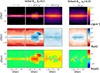 |
Fig. 24. Rendering of density, magnetic field strength, and vertical magnetic field of the early starburst period for the initial low central plasma beta simulation (β0, center = 0.1), which shows the ejection of magnetic flux during this time. This results in a more magnetized CGM than a simulation that amplifies from a much weaker initial magnetic field. However, both the cases can be seen to develop a similar vertical structure around the central disk. |
4. Discussion
In this paper, we performed simulations of isolated Milky-Way type galaxies using smoothed particle magnetohydrodynamics with a large range of different numerical parameters, such as SN feedback, resolution, Jeans floor, diffusion parameters, and initial conditions. Looking at how each of these parameters affects the growth and saturation of the magnetic field.
Regions of the galaxy with an effective dynamo, saturate their magnetic fields with values ranging from 1 − 100 μG. The average saturation of the whole central disk lies around 2 − 5 μG, which is similar to the strength observed in the main body of the Milky Way disk and similar galaxies (Taylor et al. 2009; Jansson & Farrar 2012a,b; Beck et al. 2016). This corresponds to an energy density at levels between 10 and 30% of the thermal energy density. Increases in resolution and decreases in the numerical resistivity showed increased average saturation levels in the central disk, indicating nonconvergence in the saturation level. Similar nonconvergence was found for amplification rates, which continuously grew with increases in resolution. Simulations with feedback have saturation times in the ranges of 0.4 Gyr–2 Gyr. For our simulations, we see no significant variation in the global star formation rates, this agrees with some previous studies (Rieder & Teyssier 2017a; Su et al. 2018; Whitworth et al. 2023) and contradict some previous studies (Pakmor & Springel 2013; Birnboim et al. 2015). The magnetic pressure is only a few percentage of the turbulent pressure in our simulations, which is not enough to significantly increase the vertical pressure support and decrease star formation. The saturation and growth rates are generally in agreement with past numerical simulations of MW-like isolated galaxies (Pakmor & Springel 2013; Rieder & Teyssier 2016; Butsky et al. 2017; Su et al. 2018; Steinwandel et al. 2019). For our no-feedback runs with NJ = 8, a 3−4 order of magnitude increase was seen for the magnetic field after around 500 Myr, which is similar to the amplification seen by Wang & Abel (2009) that did not include feedback in their runs.
In most of our simulations, we see a decrease in magnetic field strength for the central region. This has been seen in previous galaxy simulations (Kotarba et al. 2009; Dobbs et al. 2016; Rieder & Teyssier 2017a; Kannan et al. 2019). There are, however, simulations that on the contrary produce very strong central magnetic fields (Kotarba et al. 2009; Pakmor & Springel 2013; Butsky et al. 2017; Steinwandel et al. 2019). In the case of Butsky et al. (2017), they include magnetic field injection during feedback events, which increases the magnetic field production within the central region of the galaxy. In addition, the galaxy that is simulated is relatively cold with very few outflows, making it more comparable to our no-feedback runs. For Pakmor & Springel (2013), it was shown by Mocz et al. (2016) that this strong central amplification is removed when using the method of constrained transport to take care of the divergence error. The work of Kotarba et al. (2009) and Steinwandel et al. (2019) stem from the same SPH implementation of magnetic fields (Dolag & Stasyszyn 2009)10 and it is interesting to discuss the potential differences between our code and theirs. First of all, similar to Pakmor & Springel (2013), the Powell method (Powell et al. 1999) is used to take care of the divergence11. The magnetic diffusion within this code is done in two-part, first, a consistent magnetic diffusion is used, which is similar to ours, but with a different signal speed. The second diffusion operation done by the code is a kernel smoothing of the magnetic field every X timestep (X is a free parameter, but 15−20 in Dolag & Stasyszyn 2009) to remove small-scale fluctuations, which is not a conservative operation. In Kotarba et al. (2009) central disk amplification seems to be related to the divergence error, and we can reproduce this central amplification if we remove the divergence cleaning and reduce the artificial resistivity of our Low resolution runs. Though the field looks noisier than Kotarba et al. (2009), likely due to the neglect of the extra smoothing operation applied in these simulations. We find average divergence errors in the order of around 10−1, which are reduced with increased resolution. The increase in Jeans floor can also be seen to result in lower divergence errors, as it results in smoother structure and better-resolved gradients, that in turn causes less divergence errors to be produced. The divergence errors seen in our simulations are comparable or better than previous Lagrangian codes, which usually lie in the range ϵdiv, B = 10−1 ↔ 101 (Kotarba et al. 2009; Pakmor & Springel 2013; Dobbs et al. 2016; Steinwandel et al. 2019). Another form for the divergence estimate was presented in Steinwandel et al. (2022) (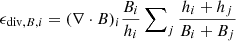 ), and the authors suggest that this form provides a more fair estimate of the error than the regular estimate of Eq. (12). We disagree with this, as this added weighting does not make it dimensionless and biases the calculation giving a much lower divergence error than in actuality. It is also seen in some work that the mean of ∇ ⋅ B is used (Pakmor & Springel 2013; Steinwandel et al. 2022), which is fairly redundant in Lagrangian codes that use the Powell method, as the total volume integral of ∇ ⋅ B across the simulation is constructed to be conserved in this method. In addition, the real measure of the ∇ ⋅ B error should be obtained by using the same gradient operator that is used in the magneto-hydrodynamic equations of the simulation. Using a higher order gradient estimator for this quantity than the one used in the induction equation of the simulation is likely to bias the analysis.
It is clear that we have an active mean-field dynamo in many of our simulations. Within the gravitational unstable no-feedback runs this mean-field dynamo acts strongly in the filamentary structure between the generated fragments. The developed structure in the disk depends strongly on the cooling and the Jeans floor. For an effective amplification of the magnetic field, we find a “Goldilocks zone” in the Jeans floor where the disk fragments but retains enough interconnectivity between the generated fragments to activate the dynamo. This is similar to the recently described GI-dynamo process (Riols & Latter 2019), where amplification occurs due to the vertical velocity rolls generated during spiral arm compression, which was found to be strongly dependent on the cooling. In Riols & Latter (2019), the authors find that amplification is hindered when the magnetic Reynolds number is increased above 100, due to the small-scale structure being generated within the spiral arms. In our case, the magnetic Reynolds number is generally below this for our no-feedback simulations. It would be interesting to run a no-feedback case at a much higher resolution to see if we also see this small-scale structure form, and if it can dampen the generated mean-field.
The addition of feedback changes the amplification processes, the spiral arm structure is continuously disturbed by the feedback and there can be a significant transfer of magnetic flux outward to the CGM. We found that, with sufficient resolution (high enough magnetic Reynolds number), the dynamo acts effectively in the disk given that the Jeans floor is small enough to not excessively suppress the collapse of gas into stars (removing the effect of feedback). For the magnetic field within the disk, the amplification is faster when the feedback is less disruptive to the ISM, and this is shown in the comparison between the blastwave and superbubble feedback models. The blastwave model generates hotter, faster winds that leaves the galaxy, and thus a relatively thin, smoother disk, whereas the superbubble model has a larger mass-loading and generates more “fountain” motions close to the galaxy, and thus increases the turbulence in the ISM and thicker disk. As a result, the blastwave model exhibits a faster amplification. However, the radial extent and maximum amplification level appear to be higher in the superbubble models in the converged runs (see Fig. 18), likely because it provides a more sustained injection of vertical motions, which enhances the dynamo. It is clear from Fig. 19 that the magnetic energy density is correlated with the turbulent density. This is in agreement with the analytical behavior of the αΩ dynamo (Ruzmaikin & Shukurov 1981; Ruzmaikin et al. 1988; Brandenburg & Subramanian 2005), where the radial extent of the magnetic field increases with increasing disk scale-height. Nevertheless, we note that increased turbulence also enhances diffusion, leading to more dissipation. In general, in a complex system like the galactic disk, the dependencies of dynamo processes on feedback can be highly nonlinear. To further disentangle the dynamo processes active in these simulations would require a full mean-field analysis, which we leave for future work.
As our simulations are isolated disks and do not have a realistic CGM component in the initial condition, the magnetization of the CGM is largely through the advection of magnetic fields by galactic winds. Faster winds generally produce a larger magnetic field in the distant CGM (e.g., the blastwave model). However, the CGM closer to the galaxy sees higher magnetic field in all runs with slower winds. This can simply be because there is more gas closer to the galaxies in these models, but it is also very likely that local amplification occurs in the CGM, which in turn enhances dynamos within the disk plane, as indicated in our highest resolution runs (Fig. 9). In nature, the CGM in a cosmological environment also includes strong accretion flows which interact with galactic outflows, together with instability processes, where the magnetic field may play an important role as well (McCourt et al. 2015). In this regard, cosmological simulations are perhaps more appropriate to study the CGM. However, as the CGM is generally much less resolved than the disk, it is unclear whether dynamos in the CGM can occur in state-of-the-art cosmological runs (which have mass resolution close to our Medium resolution cases). We defer a more detailed study of the magnetic field in the CGM in future work.
From the simulations, we could see that the density-averaged numerical Prandtl number is found to be below unity throughout the galaxy for all our simulations, with an increasing value with radius. It is clear that the Prandtl number is highly dependent on the underlying fluid environment. Early times (0.25 Gyr) in the galaxy evolution, the Prandtl number seems to be fairly independent of the resolution, while in later times (2 Gyr), it shows a slight increase with resolution. Previous studies done in shearing boxes with subsonic flow using the same code have shown a slight increase in the Prandtl number with resolution (Wissing et al. 2022). In Tricco et al. (2016b), they find that the Prandtl number decreases with resolution in supersonic turbulent box simulations12. An interesting follow-up work would be to further look into how the numerical Prandtl number changes as we go from subsonic to supersonic for different environments and to potentially modify the numerical scheme to produce a higher and more independent Prandtl number. This would be highly desirable as the Prandtl number can determine the growth and saturation level of many dynamo processes (Schekochihin et al. 2004; Federrath et al. 2014; Wissing et al. 2022). The magnetic Reynolds number is within the range of (Remag = 10 − 200) for all the simulations, which is comparatively low compared to the levels potentially required for the small-scale dynamo (Remag = 30 − 4000). However, this depends on the assumptions of the turbulence injection length and the velocity dispersion at that scale, which we have taken to be linj = 1 kpc and σv, inj = vturb, respectively.
Fourier analysis was performed for a 10 kpc cube region of the galaxy in order to investigate the relative solenoidal to compressive ratio for the velocity field (Eq. (21) with A = v). We find that, assuming a turbulent injection scale of 1 kpc, we get a natural mixture value between Ekin, ratio = 0.5 − 0.65 across our simulations, which is in accordance with the predicted natural mixture of 3D turbulence (Elmegreen & Scalo 2004; Federrath et al. 2008). While this indicates that we resolve the energy transfer between compressional and solenoidal modes in our simulations, it is too early to draw this conclusion due to the range of inertial scales and turbulent injection scales covered within the simulation. Local simulations looking at the turbulence injection length and mixture of solenoidal to compressive modes remain untested for the blastwave and the superbubble model. These would be important to get a better grasp of what the critical Reynolds number is for the small-scale dynamo of these models. Ideally, this would be tested using different boundary conditions as well (periodic, open, shear boundaries), as we know that flow conditions such as shear and vertical motions will affect both the active dynamo processes.
In conclusion, we find that:
-
The results show a strong mean-field dynamo occurring in the spiral-arm region of the disk, related to an alpha-omega-type dynamo, either by the classical alpha-omega effect or the recently described GI dynamo.
-
Without star formation and feedback, the amplification is highly determined by the degree of fragmentation within the disk which is set by the cooling and the Jeans floor. The highest amplification can be seen in the case of NJ = 8 for our low-resolution runs. Amplification is driven by shear and vertical motions within the filamentary structure that forms around and between fragments (αΩ effect). Higher NJ generally leads to less collapse and less amplification, and lower NJ leads to too much fragmentation, decreasing the filamentary structure between fragments.
-
The inclusion of feedback is seen to work in both a destructive and positive fashion for the amplification process. Destructive interference for the amplification occurs due to the increase of turbulent diffusion within the disk and the ejection of magnetic flux from the central plane to the CGM. The positive effect of feedback is the increase in vertical motions and the turbulent fountain flows that develop. The effective amplification is highly dependent on the small-scale vertical structure and the numerical dissipation within the galaxy, making the amplification highly dependent on resolution and the numerical dissipation parameters. Galaxies with an effective dynamo saturate their magnetic energy density at levels between 10 and 30% of the thermal energy density.
-
For the same feedback model and injection length, the amplification rate within the central disk reduces for stronger feedback (higher ϵSN) runs, mainly due to an increase in scale height of the galaxy. This, however, leads to higher saturation of magnetic fields within the CGM, which can be shown to be directly correlated to the increase in turbulent energy density of the CGM. Given that the resolution is high enough, the saturation level within the central disk remains fairly independent of the feedback strength.
-
It is clear from our results that the low-resolution simulations do not show the same converged behavior as the medium resolution. This points to a failure to resolve the relevant amplification processes in the low-resolution simulations, either due to reduced dynamo efficiency or to too much disruption and diffusion within the central disk.
-
Increasing the coupling and injection length of the superbubble feedback can be seen to have a positive effect on the magnetic field amplification. Potentially this is due to three effects: first, it can be seen to produce larger bubble regions, which would indicate a larger turbulent injection length, which results in higher effective Reynolds numbers. Second, gradients become smoother and thereby more resolved. Third, the more “gentle” galactic winds produced at higher injection lengths distribute gas closer to the disk, leading to more large-scale eddies being resolved in the vertical direction.
-
The blastwave scheme produces faster amplification than the superbubble scheme. The reason for this is harder to distinguish; however, we can see that a blastwave generates a more compact and smooth inner structure where the majority of the amplification takes place. Thus, it can reduce turbulent diffusion and dissipation of the magnetic field. The blastwave model also produces hotter winds than the superbubble model; these winds are fast but contain much less mass than the winds in the superbubble model. This leads to a reduced rate of advection of magnetic fields away from the central disk region, compared to the superbubble model.
-
Due to the strong initial starburst within the galaxy the initial magnetic flux is ejected from the central disk to the CGM. This makes the subsequent evolution independent of the magnetic field geometry, where similar growth was seen for both an initial vertical field and an initial toroidal field. Stronger initial field strengths can be seen to disperse their initial flux from the central disk and saturate to a level comparable to galaxies that resolve the amplification process and amplify from a much weaker initial field strength.
-
The density-averaged numerical Prandtl number is found to be below unity throughout the galaxy for all our simulations, with an increasing value with radius. During the early starburst period of the galaxy, the Prandtl number seems to be fairly independent of the resolution, while at later times (2 Gyr) we can see an increase in its value due to resolution. Previous studies have shown that in subsonic flow, the Prandtl number increases with the resolution for SPH (Wissing et al. 2022), indicating a change in behavior for supersonic shearing flows. The magnetic Reynolds number is within the range of (Remag = 10 − 200), which is comparatively low compared to the levels potentially required for the small-scale dynamo (Remag = 30 − 4000). However, this depends on the assumptions of the turbulence injection length and the velocity dispersion at that scale, which we have taken to be 1 kpc and vturb, respectively.
Mocz et al. (2016) have shown that an implementation of constrained transport scheme with moving meshes is possible, though being limited to global time-stepping.
By traditional SPH we mean the MHD equations that are derived directly from the Euler–Lagrange equations with the traditional SPH density estimate ρa = ∑bmbWab. See Price (2012) for more information.
Potentially one can also use the density scaling ρ1/3vturb and ρ1/3valf, which given that turbulence is saturated leads to the original Kolmogorov (1941) scaling for the kinetic turbulence. This is because within the inertial range, this density scaling ensures a constant energy flux (Kritsuk et al. 2007).
While the magnetic field methodology is the same between the two works (Kotarba et al. 2009; Steinwandel et al. 2019), Steinwandel et al. (2019) uses the updated GADGET3 SPH improvements of Beck et al. (2016) for their full MHD equations.
It is sometimes referred to as Powell cleaning, though there is no cleaning field introduced in this method. This is a zeroth-order cleaning as the method simply means removing the monopole currents from the induction equation, leading to the divergence errors to advect with the flow of the fluid ensuring that the surface integral of the magnetic field is conserved (Janhunen 2000; Dellar 2001).
Acknowledgments
We thank the anonymous referee for the valuable suggestions which have improved the quality and clarity of the paper. We thank James Wadsley and Benjamin Keller for providing the isolated disk initial conditions and for the insightful discussions during the project. The simulations were performed using the resources from the National Infrastructure for High Performance Computing and Data Storage in Norway, UNINETT Sigma2, allocated to Project NN9477K. We also acknowledge the support from the Research Council of Norway through NFR Young Research Talents Grant 276043.
References
- Aarseth, S. J., & Fall, S. M. 1980, ApJ, 236, 43 [NASA ADS] [CrossRef] [Google Scholar]
- Adebahr, B., Krause, M., Klein, U., et al. 2013, A&A, 555, A23 [NASA ADS] [CrossRef] [EDP Sciences] [Google Scholar]
- Alexakis, A., Mininni, P. D., & Pouquet, A. 2006, ApJ, 640, 335 [NASA ADS] [CrossRef] [Google Scholar]
- Balsara, D. S., Kim, J., Mac Low, M.-M., & Mathews, G. J. 2004, ApJ, 617, 339 [NASA ADS] [CrossRef] [Google Scholar]
- Bate, M. R., & Burkert, A. 1997, MNRAS, 288, 1060 [NASA ADS] [CrossRef] [Google Scholar]
- Beck, R. 2007, A&A, 470, 539 [NASA ADS] [CrossRef] [EDP Sciences] [Google Scholar]
- Beck, R. 2015, A&ARv, 24, 4 [Google Scholar]
- Beck, R., & Wielebinski, R. 2013, in Magnetic Fields in Galaxies, eds. T. D. Oswalt, & G. Gilmore (Springer), 5, 641 [Google Scholar]
- Beck, R., Brandenburg, A., Moss, D., Shukurov, A., & Sokoloff, D. 1996, ARA&A, 34, 155 [NASA ADS] [CrossRef] [Google Scholar]
- Beck, M. C., Beck, A. M., Beck, R., et al. 2016, JCAP, 2016, 056 [CrossRef] [Google Scholar]
- Benincasa, S. M., Tasker, E. J., Pudritz, R. E., & Wadsley, J. 2013, ApJ, 776, 23 [NASA ADS] [CrossRef] [Google Scholar]
- Bernet, M. L., Miniati, F., Lilly, S. J., Kronberg, P. P., & Dessauges-Zavadsky, M. 2008, Nature, 454, 302 [NASA ADS] [CrossRef] [Google Scholar]
- Bieri, R., Naab, T., Geen, S., et al. 2022, MNRAS, submitted [arXiv:2209.06842] [Google Scholar]
- Birnboim, Y., Balberg, S., & Teyssier, R. 2015, MNRAS, 447, 3678 [NASA ADS] [CrossRef] [Google Scholar]
- Bisnovatyi-Kogan, G. S., Ruzmaikin, A. A., & Syunyaev, R. A. 1973, Soviet Astron., 17, 137 [NASA ADS] [Google Scholar]
- Blackman, E. G., & Brandenburg, A. 2002, ApJ, 579, 359 [NASA ADS] [CrossRef] [Google Scholar]
- Booth, C. M., Agertz, O., Kravtsov, A. V., & Gnedin, N. Y. 2013, ApJ, 777, L16 [CrossRef] [Google Scholar]
- Boulares, A., & Cox, D. P. 1990, ApJ, 365, 544 [NASA ADS] [CrossRef] [Google Scholar]
- Brandenburg, A., & Sandin, C. 2004, A&A, 427, 13 [NASA ADS] [CrossRef] [EDP Sciences] [Google Scholar]
- Brandenburg, A., & Subramanian, K. 2005, Phys. Rep., 417, 1 [NASA ADS] [CrossRef] [Google Scholar]
- Brandenburg, A., Kahniashvili, T., & Tevzadze, A. G. 2015, Phys. Rev. Lett., 114, 075001 [NASA ADS] [CrossRef] [Google Scholar]
- Breitschwerdt, D., de Avillez, M. A., Fuchs, B., & Dettbarn, C. 2009, Space Sci. Rev., 143, 263 [NASA ADS] [CrossRef] [Google Scholar]
- Burlaga, L. F., Ness, N. F., & Stone, E. C. 2013, Science, 341, 147 [NASA ADS] [CrossRef] [Google Scholar]
- Butsky, I. S., & Quinn, T. R. 2018, ApJ, 868, 108 [NASA ADS] [CrossRef] [Google Scholar]
- Butsky, I., Zrake, J., Kim, J.-H., Yang, H.-I., & Abel, T. 2017, ApJ, 843, 113 [NASA ADS] [CrossRef] [Google Scholar]
- Chabrier, G. 2003, PASP, 115, 763 [Google Scholar]
- Chen, Y.-M., Tremonti, C. A., Heckman, T. M., et al. 2010, AJ, 140, 445 [Google Scholar]
- Chiaki, G., & Yoshida, N. 2015, MNRAS, 451, 3955 [NASA ADS] [CrossRef] [Google Scholar]
- Chyży, K. T., & Beck, R. 2004, A&A, 417, 541 [NASA ADS] [CrossRef] [EDP Sciences] [Google Scholar]
- Chyży, K. T., Bomans, D. J., Krause, M., et al. 2007, A&A, 462, 933 [NASA ADS] [CrossRef] [EDP Sciences] [Google Scholar]
- Cicone, C., Maiolino, R., Sturm, E., et al. 2014, A&A, 562, A21 [NASA ADS] [CrossRef] [EDP Sciences] [Google Scholar]
- de Avillez, M. A., & Breitschwerdt, D. 2005, A&A, 436, 585 [NASA ADS] [CrossRef] [EDP Sciences] [Google Scholar]
- de Avillez, M. A., & Breitschwerdt, D. 2007, ApJ, 665, L35 [NASA ADS] [CrossRef] [Google Scholar]
- Dehnen, W. 2002, J. Comput. Phys., 179, 27 [NASA ADS] [CrossRef] [Google Scholar]
- Dellar, P. J. 2001, J. Comput. Phys., 172, 392 [NASA ADS] [CrossRef] [Google Scholar]
- Del Sordo, F., & Brandenburg, A. 2011, A&A, 528, A145 [NASA ADS] [CrossRef] [EDP Sciences] [Google Scholar]
- Deng, H., Mayer, L., Latter, H., Hopkins, P. F., & Bai, X.-N. 2019, ApJS, 241, 26 [NASA ADS] [CrossRef] [Google Scholar]
- Di Matteo, T., Springel, V., & Hernquist, L. 2005, Nature, 433, 604 [NASA ADS] [CrossRef] [Google Scholar]
- Dobbs, C. L. 2008, MNRAS, 391, 844 [NASA ADS] [CrossRef] [Google Scholar]
- Dobbs, C. L., & Bonnell, I. A. 2008, MNRAS, 385, 1893 [NASA ADS] [CrossRef] [Google Scholar]
- Dobbs, C. L., Price, D. J., Pettitt, A. R., Bate, M. R., & Tricco, T. S. 2016, MNRAS, 461, 4482 [NASA ADS] [CrossRef] [Google Scholar]
- Dolag, K., & Stasyszyn, F. 2009, MNRAS, 398, 1678 [NASA ADS] [CrossRef] [Google Scholar]
- Durrer, R., & Neronov, A. 2013, A&ARv, 21, 62 [NASA ADS] [CrossRef] [Google Scholar]
- El-Badry, K., Ostriker, E. C., Kim, C.-G., Quataert, E., & Weisz, D. R. 2019, MNRAS, 490, 1961 [CrossRef] [Google Scholar]
- Elmegreen, B. G., & Burkert, A. 2010, ApJ, 712, 294 [Google Scholar]
- Elmegreen, B. G., & Scalo, J. 2004, ARA&A, 42, 211 [Google Scholar]
- Evans, C. R., & Hawley, J. F. 1988, ApJ, 332, 659 [Google Scholar]
- Federrath, C. 2016, J. Plasma Phys., 82, 535820601 [Google Scholar]
- Federrath, C., Klessen, R. S., & Schmidt, W. 2008, ApJ, 688, L79 [NASA ADS] [CrossRef] [Google Scholar]
- Federrath, C., Roman-Duval, J., Klessen, R. S., Schmidt, W., & Mac Low, M. M. 2010, A&A, 512, A81 [NASA ADS] [CrossRef] [EDP Sciences] [Google Scholar]
- Federrath, C., Chabrier, G., Schober, J., et al. 2011a, Phys. Rev. Lett., 107, 114504 [NASA ADS] [CrossRef] [Google Scholar]
- Federrath, C., Sur, S., Schleicher, D. R. G., Banerjee, R., & Klessen, R. S. 2011b, ApJ, 731, 62 [NASA ADS] [CrossRef] [Google Scholar]
- Federrath, C., Schober, J., Bovino, S., & Schleicher, D. R. G. 2014, ApJ, 797, L19 [NASA ADS] [CrossRef] [Google Scholar]
- Fletcher, A. 2010, ASP Conf. Ser., 438, 197 [NASA ADS] [Google Scholar]
- Fletcher, A., Beck, R., Shukurov, A., Berkhuijsen, E. M., & Horellou, C. 2011, MNRAS, 412, 2396 [CrossRef] [Google Scholar]
- Frick, P., Stepanov, R., Beck, R., et al. 2016, A&A, 585, A21 [NASA ADS] [CrossRef] [EDP Sciences] [Google Scholar]
- Frisch, U. 1995, Turbulence: The Legacy of A.N. Kolmogorov (Cambridge: Cambridge University Press) [CrossRef] [Google Scholar]
- Frisch, U., Pouquet, A., Leorat, J., & Mazure, A. 1975, J. Fluid Mech., 68, 769 [NASA ADS] [CrossRef] [Google Scholar]
- Fromang, S., Papaloizou, J., Lesur, G., & Heinemann, T. 2007, A&A, 476, 1123 [NASA ADS] [CrossRef] [EDP Sciences] [Google Scholar]
- Gent, F. A., Shukurov, A., Fletcher, A., Sarson, G. R., & Mantere, M. J. 2013, MNRAS, 432, 1396 [NASA ADS] [CrossRef] [Google Scholar]
- Gritschneder, M., Naab, T., Walch, S., Burkert, A., & Heitsch, F. 2009, ApJ, 694, L26 [NASA ADS] [CrossRef] [Google Scholar]
- Gutcke, T. A., Pakmor, R., Naab, T., & Springel, V. 2021, MNRAS, 501, 5597 [NASA ADS] [Google Scholar]
- Haardt, F., & Madau, P. 1996, ApJ, 461, 20 [Google Scholar]
- Hanasz, M., Wóltański, D., & Kowalik, K. 2009, ApJ, 706, L155 [NASA ADS] [CrossRef] [Google Scholar]
- Hanayama, H., Takahashi, K., Kotake, K., et al. 2005, ApJ, 633, 941 [NASA ADS] [CrossRef] [Google Scholar]
- Haugen, N. E., Brandenburg, A., & Dobler, W. 2004a, Phys. Rev. E, 70, 016308 [NASA ADS] [CrossRef] [Google Scholar]
- Haugen, N. E. L., Brandenburg, A., & Mee, A. J. 2004b, MNRAS, 353, 947 [Google Scholar]
- Heesen, V., Beck, R., Krause, M., & Dettmar, R. J. 2011, A&A, 535, A79 [NASA ADS] [CrossRef] [EDP Sciences] [Google Scholar]
- Heesen, V., Brinks, E., Leroy, A. K., et al. 2014, AJ, 147, 103 [NASA ADS] [CrossRef] [Google Scholar]
- Heinemann, T., McWilliams, J. C., & Schekochihin, A. A. 2011, Phys. Rev. Lett., 107, 255004 [NASA ADS] [CrossRef] [Google Scholar]
- Hislop, J. M., Naab, T., Steinwandel, U. P., et al. 2022, MNRAS, 509, 5938 [Google Scholar]
- Hollins, J. F., Sarson, G. R., Shukurov, A., Fletcher, A., & Gent, F. A. 2017, ApJ, 850, 4 [NASA ADS] [CrossRef] [Google Scholar]
- Hoyle, F. 1953, ApJ, 118, 513 [NASA ADS] [CrossRef] [Google Scholar]
- Hu, C.-Y. 2019, MNRAS, 483, 3363 [NASA ADS] [CrossRef] [Google Scholar]
- Hu, C.-Y., Naab, T., Walch, S., Glover, S. C. O., & Clark, P. C. 2016, MNRAS, 458, 3528 [CrossRef] [Google Scholar]
- Janhunen, P. 2000, J. Comput. Phys., 160, 649 [NASA ADS] [CrossRef] [Google Scholar]
- Jansson, R., & Farrar, G. R. 2012a, ApJ, 757, 14 [NASA ADS] [CrossRef] [Google Scholar]
- Jansson, R., & Farrar, G. R. 2012b, ApJ, 761, L11 [NASA ADS] [CrossRef] [Google Scholar]
- Joung, M. K. R., & Mac Low, M.-M. 2006, ApJ, 653, 1266 [NASA ADS] [CrossRef] [Google Scholar]
- Jun, B.-I., Norman, M. L., & Stone, J. M. 1995, ApJ, 453, 332 [Google Scholar]
- Kannan, R., Vogelsberger, M., Marinacci, F., et al. 2019, MNRAS, 485, 117 [CrossRef] [Google Scholar]
- Katz, N. 1992, ApJ, 391, 502 [NASA ADS] [CrossRef] [Google Scholar]
- Keller, B. W., Wadsley, J., Benincasa, S. M., & Couchman, H. M. P. 2014, MNRAS, 442, 3013 [NASA ADS] [CrossRef] [Google Scholar]
- Keller, B. W., Wadsley, J., & Couchman, H. M. P. 2015, MNRAS, 453, 3499 [Google Scholar]
- Kim, C.-G., & Ostriker, E. C. 2015, ApJ, 802, 99 [NASA ADS] [CrossRef] [Google Scholar]
- Kim, J.-H., Abel, T., Agertz, O., et al. 2014, ApJS, 210, 14 [Google Scholar]
- Klessen, R. S., & Hennebelle, P. 2010, A&A, 520, A17 [NASA ADS] [CrossRef] [Google Scholar]
- Kolmogorov, A. 1941, Dokl. Akad. Nauk SSSR, 30, 301 [NASA ADS] [Google Scholar]
- Kotarba, H., Lesch, H., Dolag, K., et al. 2009, MNRAS, 397, 733 [NASA ADS] [CrossRef] [Google Scholar]
- Kritsuk, A. G., Norman, M. L., Padoan, P., & Wagner, R. 2007, ApJ, 665, 416 [NASA ADS] [CrossRef] [Google Scholar]
- Krumholz, M. R., Matzner, C. D., & McKee, C. F. 2006, ApJ, 653, 361 [NASA ADS] [CrossRef] [Google Scholar]
- Lahén, N., Naab, T., Johansson, P. H., et al. 2020, ApJ, 891, 2 [CrossRef] [Google Scholar]
- Lazar, M., Schlickeiser, R., Wielebinski, R., & Poedts, S. 2009, ApJ, 693, 1133 [NASA ADS] [CrossRef] [Google Scholar]
- Lee, E. J., Murray, N., & Rahman, M. 2012, ApJ, 752, 146 [NASA ADS] [CrossRef] [Google Scholar]
- Leroy, A. K., Walter, F., Martini, P., et al. 2015, ApJ, 814, 83 [Google Scholar]
- Lesaffre, P., & Balbus, S. A. 2007, MNRAS, 381, 319 [NASA ADS] [CrossRef] [Google Scholar]
- Lesch, H., & Hanasz, M. 2003, A&A, 401, 809 [NASA ADS] [CrossRef] [EDP Sciences] [Google Scholar]
- Lodato, G., & Price, D. J. 2010, MNRAS, 405, 1212 [NASA ADS] [Google Scholar]
- Mac Low, M.-M., & Klessen, R. S. 2004, Rev. Mod. Phys., 76, 125 [Google Scholar]
- Marri, S., & White, S. D. M. 2003, MNRAS, 345, 561 [NASA ADS] [CrossRef] [Google Scholar]
- Martel, H., Evans, N. J., II, & Shapiro, P. R. 2006, ApJS, 163, 122 [NASA ADS] [CrossRef] [Google Scholar]
- Martin-Alvarez, S., Devriendt, J., Slyz, A., & Teyssier, R. 2018, MNRAS, 479, 3343 [NASA ADS] [CrossRef] [Google Scholar]
- Martini, P., Leroy, A. K., Mangum, J. G., et al. 2018, ApJ, 856, 61 [Google Scholar]
- McCourt, M., O’Leary, R. M., Madigan, A.-M., & Quataert, E. 2015, MNRAS, 449, 2 [NASA ADS] [CrossRef] [Google Scholar]
- McKee, C. F. 1989, ApJ, 345, 782 [NASA ADS] [CrossRef] [Google Scholar]
- Mee, A. J., & Brandenburg, A. 2006, MNRAS, 370, 415 [NASA ADS] [Google Scholar]
- Mina, M., Shen, S., Keller, B. W., et al. 2021, A&A, 655, A22 [NASA ADS] [CrossRef] [EDP Sciences] [Google Scholar]
- Mocz, P., Pakmor, R., Springel, V., et al. 2016, MNRAS, 463, 477 [NASA ADS] [CrossRef] [Google Scholar]
- Mukherjee, D., Bicknell, G. V., Sutherland, R., & Wagner, A. 2016, MNRAS, 461, 967 [NASA ADS] [CrossRef] [Google Scholar]
- Opher, M., Bibi, F. A., Toth, G., et al. 2009, Nature, 462, 1036 [NASA ADS] [CrossRef] [Google Scholar]
- Padoan, P., Pan, L., Haugbølle, T., & Nordlund, Å. 2016, ApJ, 822, 11 [NASA ADS] [CrossRef] [Google Scholar]
- Pakmor, R., & Springel, V. 2013, MNRAS, 432, 176 [NASA ADS] [CrossRef] [Google Scholar]
- Pakmor, R., Pfrommer, C., Simpson, C. M., & Springel, V. 2016, ApJ, 824, L30 [NASA ADS] [CrossRef] [Google Scholar]
- Palenzuela, C., Aguilera-Miret, R., Carrasco, F., et al. 2022, Phys. Rev. D, 106, 023013 [NASA ADS] [CrossRef] [Google Scholar]
- Peters, T., Banerjee, R., Klessen, R. S., & Mac Low, M.-M. 2011, ApJ, 729, 72 [Google Scholar]
- Piontek, R. A., & Ostriker, E. C. 2007, ApJ, 663, 183 [NASA ADS] [CrossRef] [Google Scholar]
- Powell, K. G., Roe, P. L., Linde, T. J., Gombosi, T. I., & De Zeeuw, D. L. 1999, J. Comput. Phys., 154, 284 [NASA ADS] [CrossRef] [Google Scholar]
- Price, D. J. 2012, J. Comput. Phys., 231, 759 [NASA ADS] [CrossRef] [Google Scholar]
- Price, D. J., & Bate, M. R. 2008, MNRAS, 385, 1820 [NASA ADS] [CrossRef] [Google Scholar]
- Rees, M. J. 2005, in Magnetic Fields in the Early Universe, eds. R. Wielebinski, & R. Beck (Springer), 664, 1 [NASA ADS] [Google Scholar]
- Rieder, M., & Teyssier, R. 2016, MNRAS, 457, 1722 [NASA ADS] [CrossRef] [Google Scholar]
- Rieder, M., & Teyssier, R. 2017a, MNRAS, 471, 2674 [NASA ADS] [CrossRef] [Google Scholar]
- Rieder, M., & Teyssier, R. 2017b, MNRAS, 472, 4368 [NASA ADS] [CrossRef] [Google Scholar]
- Riols, A., & Latter, H. 2019, MNRAS, 482, 3989 [Google Scholar]
- Robertson, B., & Goldreich, P. 2012, ApJ, 750, L31 [Google Scholar]
- Robertson, B. E., & Kravtsov, A. V. 2008, ApJ, 680, 1083 [NASA ADS] [CrossRef] [Google Scholar]
- Robishaw, T., Quataert, E., & Heiles, C. 2008, ApJ, 680, 981 [NASA ADS] [CrossRef] [Google Scholar]
- Rogachevskii, I., & Kleeorin, N. 2003, Phys. Rev. E, 68, 036301 [NASA ADS] [CrossRef] [Google Scholar]
- Rogachevskii, I., & Kleeorin, N. 2004, Phys. Rev. E, 70, 046310 [NASA ADS] [CrossRef] [Google Scholar]
- Ruzmaikin, A. A., & Shukurov, A. M. 1981, Soviet Astron., 25, 553 [NASA ADS] [Google Scholar]
- Ruzmaikin, A. A., Sokolov, D. D., & Shukurov, A. M. 1988, Magnetic Fields of Galaxies (Dordrecht: Springer), 133 [Google Scholar]
- Sasao, T. 1973, PASJ, 25, 1 [NASA ADS] [Google Scholar]
- Schekochihin, A. A., Cowley, S. C., Taylor, S. F., Maron, J. L., & McWilliams, J. C. 2004, ApJ, 612, 276 [NASA ADS] [CrossRef] [Google Scholar]
- Schekochihin, A. A., Haugen, N. E. L., Brandenburg, A., et al. 2005, ApJ, 625, L115 [NASA ADS] [CrossRef] [Google Scholar]
- Schlickeiser, R. 2012, Phys. Rev. Lett., 109, 261101 [Google Scholar]
- Schlickeiser, R., & Felten, T. 2013, ApJ, 778, 39 [NASA ADS] [CrossRef] [Google Scholar]
- Schober, J., Schleicher, D., Federrath, C., et al. 2012, ApJ, 754, 99 [NASA ADS] [CrossRef] [Google Scholar]
- Shen, S., Wadsley, J., & Stinson, G. 2010, MNRAS, 407, 1581 [NASA ADS] [CrossRef] [Google Scholar]
- Silant’ev, N. A. 2000, A&A, 364, 339 [Google Scholar]
- Simon, J. B., Hawley, J. F., & Beckwith, K. 2009, ApJ, 690, 974 [NASA ADS] [CrossRef] [Google Scholar]
- Smith, M. C., Sijacki, D., & Shen, S. 2018, MNRAS, 478, 302 [NASA ADS] [CrossRef] [Google Scholar]
- Smith, M. C., Bryan, G. L., Somerville, R. S., et al. 2021, MNRAS, 506, 3882 [NASA ADS] [CrossRef] [Google Scholar]
- Springel, V. 2010, MNRAS, 401, 791 [Google Scholar]
- Springel, V., & Hernquist, L. 2003, MNRAS, 339, 289 [Google Scholar]
- Springel, V., Di Matteo, T., & Hernquist, L. 2005, MNRAS, 361, 776 [Google Scholar]
- Squire, J., & Bhattacharjee, A. 2015, Phys. Rev. Lett., 114, 085002 [NASA ADS] [CrossRef] [Google Scholar]
- Stadel, J. G. 2001, Ph.D. Thesis, University of Washington, USA [Google Scholar]
- Steinwandel, U. P., Beck, M. C., Arth, A., et al. 2019, MNRAS, 483, 1008 [NASA ADS] [CrossRef] [Google Scholar]
- Steinwandel, U. P., Moster, B. P., Naab, T., Hu, C.-Y., & Walch, S. 2020, MNRAS, 495, 1035 [NASA ADS] [CrossRef] [Google Scholar]
- Steinwandel, U. P., Böss, L. M., Dolag, K., & Lesch, H. 2022, ApJ, 933, 131 [NASA ADS] [CrossRef] [Google Scholar]
- Stinson, G., Seth, A., Katz, N., et al. 2006, MNRAS, 373, 1074 [NASA ADS] [CrossRef] [Google Scholar]
- Su, K.-Y., Hayward, C. C., Hopkins, P. F., et al. 2018, MNRAS, 473, L111 [NASA ADS] [CrossRef] [Google Scholar]
- Subramanian, K., Narasimha, D., & Chitre, S. M. 1994, MNRAS, 271, L15 [NASA ADS] [CrossRef] [Google Scholar]
- Sun, M., & Takayama, K. 2003, J. Fluid Mech., 478, 237 [NASA ADS] [CrossRef] [Google Scholar]
- Tamburro, D., Rix, H. W., Leroy, A. K., et al. 2009, AJ, 137, 4424 [Google Scholar]
- Tasker, E. J., & Tan, J. C. 2009, ApJ, 700, 358 [NASA ADS] [CrossRef] [Google Scholar]
- Taylor, A. R., Stil, J. M., & Sunstrum, C. 2009, ApJ, 702, 1230 [Google Scholar]
- Teyssier, R. 2002, A&A, 385, 337 [CrossRef] [EDP Sciences] [Google Scholar]
- Tricco, T. S., & Price, D. J. 2012, J. Comput. Phys., 231, 7214 [NASA ADS] [CrossRef] [Google Scholar]
- Tricco, T. S., Price, D. J., & Bate, M. R. 2016a, J. Comput. Phys., 322, 326 [NASA ADS] [CrossRef] [Google Scholar]
- Tricco, T. S., Price, D. J., & Federrath, C. 2016b, MNRAS, 461, 1260 [NASA ADS] [CrossRef] [Google Scholar]
- Truelove, J. K., Klein, R. I., McKee, C. F., et al. 1997, ApJ, 489, L179 [CrossRef] [Google Scholar]
- Turk, M. J., Oishi, J. S., Abel, T., & Bryan, G. L. 2012, ApJ, 745, 154 [NASA ADS] [CrossRef] [Google Scholar]
- Uhlig, M., Pfrommer, C., Sharma, M., et al. 2012, MNRAS, 423, 2374 [CrossRef] [Google Scholar]
- Vázquez-Semadeni, E., Kim, J., Shadmehri, M., & Ballesteros-Paredes, J. 2005, ApJ, 618, 344 [CrossRef] [Google Scholar]
- Vázquez-Semadeni, E., Colín, P., Gómez, G. C., Ballesteros-Paredes, J., & Watson, A. W. 2010, ApJ, 715, 1302 [CrossRef] [Google Scholar]
- Vazza, F., Brunetti, G., Brüggen, M., & Bonafede, A. 2018, MNRAS, 474, 1672 [NASA ADS] [CrossRef] [Google Scholar]
- Vishniac, E. T. 1994, ApJ, 428, 186 [Google Scholar]
- Vishniac, E. T., & Brandenburg, A. 1997, ApJ, 475, 263 [NASA ADS] [CrossRef] [Google Scholar]
- Wadsley, J. W., Stadel, J., & Quinn, T. 2004, New Astron., 9, 137 [Google Scholar]
- Wadsley, J. W., Veeravalli, G., & Couchman, H. M. P. 2008, MNRAS, 387, 427 [NASA ADS] [CrossRef] [Google Scholar]
- Wadsley, J. W., Keller, B. W., & Quinn, T. R. 2017, MNRAS, 471, 2357 [NASA ADS] [CrossRef] [Google Scholar]
- Wang, P., & Abel, T. 2009, ApJ, 696, 96 [NASA ADS] [CrossRef] [Google Scholar]
- Weaver, R., McCray, R., Castor, J., Shapiro, P., & Moore, R. 1977, ApJ, 218, 377 [Google Scholar]
- Whitworth, D. J., Smith, R. J., Klessen, R. S., et al. 2023, MNRAS, 520, 89 [NASA ADS] [CrossRef] [Google Scholar]
- Widrow, L. M. 2002, Rev. Mod. Phys., 74, 775 [NASA ADS] [CrossRef] [Google Scholar]
- Wissing, R., & Shen, S. 2020, A&A, 638, A140 [NASA ADS] [CrossRef] [EDP Sciences] [Google Scholar]
- Wissing, R., Shen, S., Wadsley, J., & Quinn, T. 2022, A&A, 659, A91 [NASA ADS] [CrossRef] [EDP Sciences] [Google Scholar]
- Zrake, J. 2014, ApJ, 794, L26 [NASA ADS] [CrossRef] [Google Scholar]
Appendix A: Dynamo or numerical amplification
Without star formation we postulate that amplification is driven by dynamo action due to shear and vertical motions within the filamentary structure that forms around and between fragments. The NJ = 10 case shown in Figure 6 is a perfect example of this as the early stage of amplification is driven by a sole fragment. While the divergence error is generally low within the clump and filament structure, it can reach quite high values within the surface shearing boundary. In this section we aim to distinguish if the growth is caused by the magnetic resistivity, divergence error or resolution at the boundary. We perform additional simulations between 700-2000 Myr of the NJ = 10 case, changing a wide range of parameters. First, we run 3 simulations varying the cleaning speed (fch = 0, 10, 100), one running with no cleaning, 10 times cleaning and 100 times cleaning13. This mainly changes the divergence error, but will also have a small effect on the dissipation of the magnetic field as this consequently increases with cleaning. The simulations in the main sections of the paper are all done with a cleaning speed of fch = 1. We run two more simulations with double and four times the artificial resistivity (αB = 1, 2). Increasing the artificial resistivity in the code greatly increases dissipation but only slightly decrease the divergence error. Finally we also increase the resolution of our Low resolution run, by splitting the particles at the time of 700 Myr, making it equivalent to the Medium resolution runs (we also alter Jeans floor so that collapse length remains the same). This causes some initial noise as particles relax, but subsequent evolution is nearly identical to the Low resolution. This improves the boundary condition and lowers both the numerical resistivity and the divergence error.
From the results we can see that the growth of the fragment and filament is mainly dependent on the resistivity and not the divergence error, this is highlighted in Figure A.1. Here we can see that, while increasing the cleaning speed does reduce the amplification of the magnetic field within the filament, it does so at a much slower rate than increasing the numerical dissipation. At the same time we can see that the divergence error is still relatively high for the high numerical dissipation case, which indicates that amplification rate is determined by numerical dissipation. Higher resolution is seen to have a positive effect on the amplification rate. However, in terms of the relative reduction in magnetic dissipation compared to the lower resolution case, it has a slower growth of the magnetic field than expected. This might indicate an additional behavior on Reynolds number/increased mixing or the Prandtl number. We have run these simulations for 2000 Myr and all cases except for the low resolution of αB = 2 (which does not amplify) see significant amplification during this time, albeit at different rates.
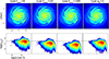 |
Fig. A.1. Results of our numerical study on the early amplification stage (t = 870 Myr) without feedback for different cleaning and numerical dissipation. Top panel shows a face-on rendering of the magnetic field strength in the galactic disk. Bottom panel shows the corresponding phase space of divergence errors for each of the four cases. We can see that increasing the cleaning speed efficiently reduces the divergence error, while still leading to amplification within the filament and fragment. In the higher numerical dissipation case (αB = 2) we can see that we still have quite high divergence error, but the amplification is reduced much more than in the fclean = 100 case. Indicating that the reduction in amplification is mainly driven by increased numerical dissipation and not divergence errors. |
All Tables
All Figures
|
Fig. 1. Face-on evolution of the no feedback simulations with varying Jeans floor and initial magnetic field geometry (B0, z two top panels, B0, ϕ bottom panel). The time for each column/Jeans floor (NJ = 4, 8, 10, 16) is t = (0.5, 1, 1, 1) Gyr respectively. The NJ = 8 case exhibits the strongest magnetic field growth at early times, likely through an active GI or αΩ dynamo within the developed filamentary structure. Further reducing the Jeans floor leads to too much fragmentation of the disk, reducing the effect of the active dynamo. For higher Jeans floor GI remain quite weak at this time, leading to either a weak amplification or decay of the magnetic field in the disk. However, in the case of the NJ = 10 and Bz, 0 where a small fragment has started to form, the disk will become unstable at a later time (see Fig. 6). |
| In the text | |
|
Fig. 2. Time evolution of the average magnetic field strength (left panel) and the normalized Maxwell stress (right panel) for the no feedback runs. Blue lines represent simulations with an initial vertical field and the red lines represent simulations with an initial toroidal field. Darker colors represent higher Jeans floor (NJ = (4, 8, 10, 16)). The NJ = 4 and NJ = 8 simulations have a rapid amplification in the magnetic field early on due to spiral arm compression. We can see that we get the strongest αMW exhibited during the growth phase of the NJ = 8 cases, correlating to the generation of radial and toroidal fields during the dynamo process. The elevated level in αMW for all the cases with an initial toroidal field is simply due to the initial field and normalization (Bz ≈ 0). |
| In the text | |
|
Fig. 3. Radial profiles of the magnetic, turbulent and thermal pressures for the no feedback runs at around t = 1 Gyr. Darker colors represents higher Jeans floor (NJ = (4, 8, 10, 16)). For the thermal pressure we only plot one line as it is similar across these simulations. For the NJ = 8 case we can see that the magnetic pressure is of similar strength as the thermal pressure in the center of the disk. The magnetic pressure decreases with radius and returns to initial values beyond 14 kpc. The turbulent pressure can be seen to significantly increases in both NJ = 4 and 8 as the disk is highly gravitationally unstable. |
| In the text | |
|
Fig. 4. Radial profile of the velocity (top), the shear parameter (middle) and the Mach number (bottom) for the NJ = 8 and NJ = 16 no-feedback runs and for the SB and BW feedback runs with NJ = 8 (light color t = 250 Myr, dark color 2 Gyr). The turbulent velocities are enhanced by the gravitational instability of the disk and the inclusion of feedback. However, BW can be seen to produce a lower turbulent response compared to SB, especially at later times (within 10 kpc). In all runs we can see that there is a reduction of the shearing parameter toward the central region, reducing the effectiveness of an αΩ type dynamo. Mach numbers are lower in the BW model due to the heating of the disk and the relatively low turbulent velocities. |
| In the text | |
|
Fig. 5. Magnetic field polarity of the NJ = 16 no feedback simulation at t = 1 Gyr with an initial vertical field. We can see field reversals throughout the disk in both the radial and toroidal directions. These are highly correlated to the spiral arm structure, as the reversals form together with the velocity perturbation induced by spiral shocks (Dobbs et al. 2016). The vertical field remains fairly correlated to the density and is similar in strength to the initial setup. |
| In the text | |
|
Fig. 6. Development of a fragment within the disk for the NJ = 10 B0, z case at later times (t = 800 − 2000 Myr), which subsequently destabilizes the disk and generates a strong magnetic field in the process. Top panel shows the density rendering and the bottom panel the magnetic field strength. |
| In the text | |
|
Fig. 7. Closer look at the magnetic field structure around the fragment at t = 1300 Myr. It is clear that the magnetic field traces the filamentary structure, with opposite/unstructured magnetic fields occurring in the low-density region around it. This is similar to the magnetic field structure formed from the GI-dynamo simulations of Riols & Latter (2019), which due to magnetic flux redistribution generates opposite radial mean fields within and outside the spiral arm. In addition, we can see that there is a strong field reversal in the gap in front of the fragment. |
| In the text | |
|
Fig. 8. Face-on rendering of the galactic disk after t = 250 Myr. Comparing the effect of resolution on the early evolution of the galaxy. Left to right goes from low to high resolution. Top panel show density, middle panel magnetic field strength and the bottom panel the toroidal magnetic field. We can see that the scale of the developed mean fields are about the same but increases in strength with resolution. |
| In the text | |
|
Fig. 9. Side-on rendering of the galactic disk after t = 250 Myr. Comparing the effect of resolution on the early evolution of the galaxy. Left to right goes from low to high resolution Top panel show density, middle panel magnetic field strength and bottom panel the toroidal magnetic field. The increase in resolution show additional the CGM. Feedback leads to the formation of an interesting vertical structure of the magnetic field, where near the central disk, we can see plenty of reversals and intricate behaviors in the magnetic field. The complexity of the structure around the central disk increases as we increase the resolution. The outer regions can be seen to be dominated by the blowout of the initial magnetic flux. |
| In the text | |
|
Fig. 10. Radial profiles of the magnetic, turbulent, and thermal pressures for the resolution study at a few different times (with later times being represented by the given color palette getting darker). For the low-resolution simulations, we did not see any significant amplification as time went by. Whereas for the medium-resolution ones, we reached a saturated state after about 1.4 Gyr. The high-resolution simulations reached a similar magnetic field strength to the medium resolution at 800 Myr after just 250 Myr. |
| In the text | |
|
Fig. 11. Mass-weighted phase diagram of the divergence error(ϵdiv, B) for the high-resolution simulation at 250 Myr. The mean divergence error is between ϵdiv, B ≈ 10−1 − 10−2. |
| In the text | |
|
Fig. 12. Face-on rendering of the magnetic field strength of galactic disk after t = 2.0 Gyr. Simulations with feedback, comparing the effect of different Jeans floor on the evolution. Top panel show the Low resolution simulation and bottom the medium resolution. We can see that we get no significant amplification in the low resolution, while strong amplification is seen in the medium resolution. Too high Jeans floor diminishes the dynamo processes as the smallest collapse length becomes too large. |
| In the text | |
|
Fig. 13. Radial profile of the energy density ratio (β−1) for the saturated medium resolution runs in Fig. 12. We have included lines for both the magnetic-thermal energy density ratio ( |
| In the text | |
|
Fig. 14. Time plots for the medium resolution feedback runs with varying Jeans floor. The left and right panel shows the evolution of Brms and αMW respectively. Darker colors represents higher Jeans floor. We can see that there is a positive dependence on the Jeans floor for the amplification rate, as long as a “critical” collapse length is resolved. The normalized Maxwell stress lie around αMW = 0.1 − 0.3 for all runs. There is additional stress within the NJ = 30 simulation during the early amplification phase with around αMW = 0.4. |
| In the text | |
|
Fig. 15. Face-on rendering of the divergence error of the magnetic field in the galactic disk after t = 2 Gyr. We can clearly see that there is a reduction in divergence error throughout the disk for higher Jeans floor. The mean divergence error in the NJ = 8 is around ϵdiv, B = 10−1 and in the NJ = 16 around ϵdiv, B = 6 × 10⁻². |
| In the text | |
|
Fig. 16. Rendering of density, magnetic field strength of the Low resolution simulations with varying feedback scheme at t = 2 Gyr. Strong field growth can be seen for both the blastwave model and the high coupling superbubble model (NFB = 200). Both the blastwave model and the physical superbubble model (NFB = 1) leads to small feedback bubbles which pushes material far away from the disk. The mass loading in the superbubble model (NFB = 1) is however much larger as the blastwave model mainly generate hot low-density outflows, this means that there is less transfer of magnetic fields from the central region in the blastwave model. Increasing the injection length (NFB = 200) leads to more mass loading, larger feedback bubbles and a more concentrated vertical structure, which in turn lead to more amplification of the magnetic field within the central disk. |
| In the text | |
|
Fig. 17. Time evolution of Brms within the central disk for different feedback schemes. Left panel show the Low resolution runs and right panel show the Medium resolution runs. Darker colors in blue and red indicate stronger feedback strength and light green represent the physical SB model (NFB = 1) and dark green represent SB model with higher coupling (NFB = 200). Its clear from both resolutions that the blastwave scheme produce faster amplification than the superbubble schemes. Higher energy injection does in general lead to slower growth of the magnetic field within the central disk. Increasing the coupling/injection length of the superbubble scheme does seem to generally have a positive effect on the magnetic field amplification. The bump seen in the NFB = 200 evolution is due to rapid amplification of the magnetic field during the merger of two fragments within the central region, which afterwards is quickly dispersed outward from the central disk. |
| In the text | |
|
Fig. 18. Rendering of density, magnetic field strength and toroidal magnetic field of the medium resolution simulations with varying feedback schemes. The blastwave model generates hotter winds and less mass loading than the superbubble model, leading to less magnetic field advection from the central plane of the disk. This generates a more radial compact structure for the magnetic field. Increasing the injection length in superbubble makes the vertical density structure more compact, leading to more resolved vertical velocity structures. In addition, we see a clear increase in the scale of the toroidal mean-field with the feedback strength as the galaxy extends both radially and vertically. |
| In the text | |
|
Fig. 19. Vertical structure of the kinetic, magnetic and thermal energy density for our medium resolution runs with varying feedback scheme around 2 Gyr. The magnetic energy density can be seen to follow the kinetic energy quite closely within the CGM. With stronger magnetic fields being present further out in the strong feedback simulations. |
| In the text | |
|
Fig. 20. Time evolution of Brms within the central disk for different numerical diffusion and resolutions. We can see that lowering the numerical diffusion has a clear positive effect on the growth rate and saturation level. Even the Low resolution reaches saturation in the case of αB = 0.25, after around 1.9 Gyr. |
| In the text | |
|
Fig. 21. Density-averaged radial profile of the fluid parameters for different resolutions and numerical diffusion at t = 2 Gyr. From top to bottom we have: the Prandtl number, the magnetic Reynolds number and the regular Reynolds number. The Prandtl number can be see to be below unity across the whole radial extent, with a decreasing trend toward the center. There is an expected increase due to lowering artificial resistivity and also an increase in Pm due to resolution in the outer regions of the disk (≥4 kpc). Both the magnetic and regular Reynolds number can be seen to increase toward the center; however, the magnetic Reynolds number remains flatter throughout the disk than its hydrodynamic counterpart. |
| In the text | |
|
Fig. 22. Density-averaged radial profile of the fluid parameters for different resolutions at an early time (t = 250 Myr αB = 0.5). From top to bottom we have: the Prandtl number, the magnetic Reynolds number and the regular Reynolds number. The Prandtl number seem to be largely independent of the resolution and mainly be effected by the conditions within the galaxy (supersonic + shear + stratified environment). Both the magnetic and regular Reynolds number can be seen to increase with a factor of 4 as we increase the resolution, which is in agreement with the expected second order of the numerical diffusion. |
| In the text | |
|
Fig. 23. Time evolution of Brms (left panel) and the vertical and toroidal fluxes (right panel) within the central disk for different initial field strengths and geometry. Darker lines represent a lower initial thermal plasma beta βth within the center of the disk. The distinct levels of initial central plasma beta are (β0, center = (107, 104, 1, 0.1)). We can see that for the low plasma beta cases (β0, center ≤ 1) the magnetic field strength is quickly reduced at the beginning of the simulation, but eventually saturates at a level around 1 μG. This is a similar saturation level as the αB = 0.25 simulations that grow from much weaker initial fields at the same resolution. Due to this outflow of magnetic flux, we can see that all simulations reduce to a similar oscillating flux within the central disk for the vertical and toroidal fields. |
| In the text | |
|
Fig. 24. Rendering of density, magnetic field strength, and vertical magnetic field of the early starburst period for the initial low central plasma beta simulation (β0, center = 0.1), which shows the ejection of magnetic flux during this time. This results in a more magnetized CGM than a simulation that amplifies from a much weaker initial magnetic field. However, both the cases can be seen to develop a similar vertical structure around the central disk. |
| In the text | |
|
Fig. A.1. Results of our numerical study on the early amplification stage (t = 870 Myr) without feedback for different cleaning and numerical dissipation. Top panel shows a face-on rendering of the magnetic field strength in the galactic disk. Bottom panel shows the corresponding phase space of divergence errors for each of the four cases. We can see that increasing the cleaning speed efficiently reduces the divergence error, while still leading to amplification within the filament and fragment. In the higher numerical dissipation case (αB = 2) we can see that we still have quite high divergence error, but the amplification is reduced much more than in the fclean = 100 case. Indicating that the reduction in amplification is mainly driven by increased numerical dissipation and not divergence errors. |
| In the text | |
Current usage metrics show cumulative count of Article Views (full-text article views including HTML views, PDF and ePub downloads, according to the available data) and Abstracts Views on Vision4Press platform.
Data correspond to usage on the plateform after 2015. The current usage metrics is available 48-96 hours after online publication and is updated daily on week days.
Initial download of the metrics may take a while.