| Issue |
A&A
Volume 682, February 2024
|
|
|---|---|---|
| Article Number | A73 | |
| Number of page(s) | 10 | |
| Section | Planets and planetary systems | |
| DOI | https://doi.org/10.1051/0004-6361/202347989 | |
| Published online | 05 February 2024 | |
Confirmation of TiO absorption and tentative detection of MgH and CrH in the atmosphere of HAT-P-41b
1
CAS Key Laboratory of Planetary Sciences, Purple Mountain Observatory, Chinese Academy of Sciences,
No. 10 Yuanhua Road, Qixia District,
210023
Nanjing,
PR China
e-mail: This email address is being protected from spambots. You need JavaScript enabled to view it.
2
School of Astronomy and Space Science, University of Science and Technology of China,
No. 96 Jinzhai Road, Baohe District,
230026
Hefei,
PR China
3
CAS Center for Excellence in Comparative Planetology,
No. 96 Jinzhai Road, Baohe District,
230026
Hefei,
PR China
4
Instituto de Astrofísica de Canarias (IAC),
Vía Láctea s/n,
38205
La Laguna,
Tenerife,
Spain
5
Departamento de Astrofísica, Universidad de La Laguna (ULL),
C/ Padre Herrera,
38206
La Laguna,
Tenerife,
Spain
Received:
15
September
2023
Accepted:
21
November
2023
Abstract
Understanding the role of optical absorbers is critical for linking the properties of the dayside and terminator atmospheres of hot Jupiters. This study aims to identify the signatures of optical absorbers in the atmosphere of the hot Jupiter HAT-P-41b. We conducted five transit observations of this planet to obtain its optical transmission spectra using the Gran Telescopio Canarias (GTC). We performed atmospheric retrievals assuming free abundances of 12 chemical species. Our Bayesian model comparisons revealed strong evidence for TiO absorption (∆ ln 𝒵 = 21.02), modest evidence for CrH (∆ ln 𝒵 = 3.73), and weak evidence for MgH (∆ ln 𝒵 = 2.32). When we combined the GTC transmission spectrum with previously published Hubble Space Telescope and Spitzer data, the retrieval results and model inferences remained consistent. In conclusion, HAT-P-41b has a metal-rich atmosphere with no high-altitude clouds or hazes. Further observations of its dayside atmosphere should be made to confirm the hints of a thermal inversion in the upper atmosphere suggested by our results.
Key words: methods: data analysis / techniques: spectroscopic / planets and satellites: atmospheres / planets and satellites: individual: HAT-P-41b
© The Authors 2024
 Open Access article, published by EDP Sciences, under the terms of the Creative Commons Attribution License (https://creativecommons.org/licenses/by/4.0), which permits unrestricted use, distribution, and reproduction in any medium, provided the original work is properly cited.
This article is published in open access under the Subscribe to Open model. This email address is being protected from spambots. You need JavaScript enabled to view it. to support open access publication.
1 Introduction
The accurate characterization of exoplanet atmospheres is crucial for solving the puzzle of planetary formation and evolution. Precise spectroscopic measurements of exoplanet atmospheres, available with current observational instruments, have mainly focused on close-in giant planets, including hot Jupiters. Certain metals, metal oxides, and hydrides have a very strong opacity in the optical wavelengths (Sharp & Burrows 2007), which can absorb the stellar radiation and heat the upper atmosphere, leading to a thermal inversion in the temperature-pressure profile and thermal emission features in the emission spectrum (Burrows et al. 2008; Guillot 2010). While it is difficult to detect optical absorbers in the emission spectrum, alkali metals (e.g., Na and K), metal oxides (e.g., TiO and VO), and hydrides (e.g., CrH and FeH) are expected to exhibit strong absorption features in the optical band of transmission spectra (Seager & Sasselov 2000; Fortney et al. 2008, 2010).
The hot Jupiter HAT-P-41b, discovered by Hartman et al. (2012), is an intriguing target for further study due to its highly inflated nature. The planet orbits an F-type star (Teff = 6390 K, M⋆ ~ 1.4 M⊙, R⋆ ~ 1.7 R⊙, [Fe/H] = 0.21) every 2.7 days and has a mass of ~0.8 MJ, a radius of ~1.7 RJ, and an equilibrium temperature of 1941 K. Wakeford et al. (2020) present a 0.2–0.8 µm transmission spectrum using the Hubble Space Telescope’s (HST) Wide Field Camera 3 (WFC3) UV/visible (UVIS) channel (G280 grism), which revealed a significant scattering slope and strong absorption features of TiO and/or VO. Lewis et al. (2020) performed retrievals on the 0.2–5.0 µm combined spectrum, consisting of HST WFC3 (G280, G141) and Spit𝒵er data, and found a potential combination of H−, CrH, AlO, VO, and Na, which would explain the ultraviolet to optical wavelengths. However, the presence of H− in the planet’s terminator atmosphere remains inconclusive (Welbanks et al. 2023). Sheppard et al. (2021) conducted a comprehensive retrieval analysis of the 0.3-5.0 µm spectrum derived from HST Space Telescope Imaging Spectrograph (STIS), HST WFC3 G141, and Spit𝒵er transit observations and found that the atmosphere of HAT-P-41b is cloud-free, haze-free, and metal-rich, with distinct water vapor absorption and tentative optical absorption. According to the emission spectrum analyses, the dayside upper atmosphere of HAT-P-41b does not exhibit strong evidence of a thermal inversion (Mansfield et al. 2021; Fu et al. 2022; Changeat et al. 2022). The observed transmission spectra suggest that optical absorbers such as metal oxides and hydrides may be present in the planet’s terminator atmosphere, but the emission spectrum did not reveal a distinct thermal inversion in the dayside atmosphere. Further confirmation and identification of the candidate optical absorbers in the atmosphere of HAT-P-41b is needed to resolve this discrepancy.
Our goal is to further investigate the atmosphere of HAT-P-41b using low-resolution transmission spectra. Multiple transit observations with the Optical System for Imaging and low-Intermediate-Resolution Integrated Spectroscopy (OSIRIS) of Gran Telescopio Canarias (GTC; Cepa et al. 2000) should enable us to obtain the optical transmission spectrum with higher photometric precision and spectral resolution than with the HST WFC3 UVIS and STIS instruments. By performing atmospheric retrievals and Bayesian model comparisons, we aim to obtain more precise estimates of the abundances of the chemical species, better constrain previously reported optical absorbers, and possibly discover new signatures in the atmosphere of HAT-P-41b.
This paper is organized as follows. We summarize the observations and the data reduction procedures in the next section. Section 3 illustrates the analysis of the GTC transit light curves. The atmospheric retrievals are demonstrated in Sect. 4. We further discuss the joint retrievals and then draw our conclusion in Sect. 5.
Input parameters of the HAT-P-41 system used in this work.
2 Observations and data reduction
We observed five transits of HAT-P-41b using the GTC OSIRIS instrument between 2013 and 2022 (hereafter OB-1 to OB-5). The observation summary is listed in Table A.1. The instrument OSIRIS has an un-vignetted field of view of 7.4′ and a pixel scale of 0.254″. Its detector consists of a mosaic of two Marconi CCDs (1024 × 2048 pixels) with a 37-pixel (9.4″) gap between them after a 2 × 2 pixel binning. The observations were performed in the long-slit spectroscopic mode with the R1000R grism covering a wavelength range of 5100–10000 Å. The gap between the CCDs was parallel to the dispersion direction and thus would not affect the spectra. We adopted a 12″ -wide slit in OB-1, OB-3, and OB-4, and a 40″ -wide slit in OB-2 and OB-5 to avoid flux loss due to the partial coverage of the point spread function (PSF). A comparison star (2MASS 19493265+0439270 for OB-1, OB-3, OB-4, and OB-5; 2MASS 19494153+0437350 for OB-2; Cutri et al. 2003) was simultaneously observed with the target star through the slit in the five observations.
The data were reduced following the methods described in our previous work (Jiang et al. 2022) to produce the spec-troscopic light curves with 5-nm passbands from 521.8 nm to 922.4 nm, where the passband of 756.8–767.4 nm covering the
telluric oxygen A band was discarded in subsequent analysis due to the very-low signal-to-noise ratio. The broadband light curves (i.e., white-light curves) were obtained in the same manner but integrated from 521.8 nm to 922.4 nm excluding the oxygen A band.
3 Light curve analysis
3.1 Transit model
We employed the Python package PyTransit (Parviainen 2015) to model the transit light curves, assuming circular orbits. There are five transit parameters in the model: the planet-to-star radius ratio (Rp/Rs), normalized orbital semimajor axis (a/R⋆), orbital inclination (i), central transit epoch (tc), and orbital period (P). For each transit, the light curves were fit separately.
For broadband light curve fitting, we employed a four-parameter nonlinear stellar limb darkening law. The limb darkening coefficients (u1 to u4) were derived using LDTK (Parviainen & Aigrain 2015) and kept fixed in light curve fitting. The orbital period was determined based on the transit ephemeris updated by Wakeford et al. (2020), with the central epoch of each transit being a free parameter under a uniform prior. To avoid systematic biases in the transmission spectra and to facilitate subsequent joint atmospheric retrievals with the transmission spectra provided by Sheppard et al. (2021), we adopted the orbital semimajor axis and inclination values consistent with those used in Sheppard et al. (2021). Furthermore, we used the broadband radius ratio measured with HST STIS G750L (Rp/Rs = 0.10159 ± 0.00042, Sheppard et al. 2021), which essentially matches the wavelength coverage of OSIRIS R1000R, as the Gaussian prior for the broadband radius ratio. This was done to ensure consistency across the five transit observations and to obtain precise central transit epochs and broadband systematic noise. Table 1 shows the adopted parameters of the HAT-P-41 system.
We performed separate fittings for the narrowband light curve in each passband. The parameter settings for the narrowband fitting were kept consistent with those of the broadband, with the exception of Rp and Tc. The radius ratio was treated as a free parameter under a uniform prior, while the central epoch of each transit was fixed to the best-fit value derived from the broadband light curve fitting. To mitigate the impact of wavelength-independent systematic noise (i.e., common-mode systematics) and enhance the precision of the derived transmission spectra, we employed the common-mode correction method outlined in Gibson et al. (2013). This involved dividing the best-fit broadband light curve by the best-fit transit model to obtain the common-mode systematics. Each narrowband light curve was then divided by the common-mode systematics to apply this correction. We note that Gibson et al. (2013) used the Gaussian process (GP) systematics plus one to approximate the common mode systematics, while we used the best-fit broadband light curve divided by the best-fit transit model. Given that the amplitudes of the GP systematics were much smaller than one, these two approximations are virtually indistinguishable.
3.2 Correction for the companion star contamination
Hartman et al. (2012) reported a resolved neighboring star, located ~3.56″ away and 3.5 mag fainter than HAT-P-41 in the i band. Wöllert et al. (2015) further observed, through lucky imaging, that this neighboring star has magnitude contrasts of ∆i′ = 3.65 ± 0.05 and ∆𝒵′ = 3.40 ± 0.05, and a spectral type between F5 and M2 assuming physical companionship. According to the Gaia observations (Table A.2; Gaia Collaboration 2016, 2023), these two stars share similar parallaxes, radial velocities, and proper motions, suggesting their association.
To correct the flux contamination from the companion star, we performed a supplementary observation with 10 exposures during OB-3, where the slit was aligned to the direction from HAT-P-41 to the companion star, so that the spectra of the two stars could be spatially resolved. The distance between the PSF peaks of the two stars is ~3.5″ (14 pixels). To separate the two stellar spectra, we first subtracted the mirrored non-contaminated side of the target’s PSF from the other side to obtain the companion’s spectrum. Since strong residuals existed at the peak location of the target, we fitted a Gaussian function to target’s original PSF and made a mask for regions within 4σ from the peak location. We then repaired the masked region by mirroring the non-contaminated part of the companion’s PSF on the other side. The target’s spectrum was then obtained by subtracting the extracted companion’s spectrum from the total spectrum. The companion-to-host flux ratio in each passband was then calculated based on the extracted stellar spectra. The broadband flux ratio (521.8–922.4 nm excluding the oxygen A band) was measured to be 0.03885 ± 0.00083. The narrowband flux ratios are shown in Fig. 1. When fitting the light curve in each passband, the flux dilution effect was corrected by
 (1)
(1)
where 𝓕 is the companion-to-host flux ratio and f*(t) is the light curve model without flux dilution.
We further refined the constraints on the physical parameters of the companion star by fitting the observed flux ratios with PHOENIX model spectra (Husser et al. 2013) based on the stellar parameters from Hartman et al. (2012) and parallaxes measurements from the Gaia data (Gaia Collaboration 2016, 2023). This method was detailed in Nortmann et al. (2016) and Jiang et al. (2023). Figure 1 shows the fitting results of the flux ratios. The derived effective temperature of  and radius of 0.708 ± 0.022 R⊙ suggest a K-type companion star. However, to accurately determine its gravity, mass, and spectral type, further high-resolution spectroscopic measurements are necessary.
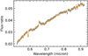 |
Fig. 1 Narrowband flux ratios between the companion and HAT-P-41. The error bars are the observed flux ratios, and the orange line is the best-fit curve obtained using the PHOENIX model spectra. |
3.3 Gaussian process modeling
The light curve systematic noise was fitted with the multi-input GP regression implemented by the Python package George (Ambikasaran et al. 2015). The GP models were applied to all the broadband and narrowband light curves individually. We adopted the 3/2-order Matérn kernel function k(r) with multi-input variables (time t, seeing1 w, and pixel drift2 p) for GP modeling:
 (2)
(2)
where  is the variance of the kernel, r is the distance between two input vectors (t, w, p) and (t + ∆t, w + ∆w, p + ∆p) normalized by the corresponding length scales ℓt, ℓw, and ℓp. In addition, the uncertainties of the normalized light curves were estimated as photon-dominated noise and usually underestimated the total white noise. To compensate for this, a jitter variance of
  was added to the diagonal of the covariance matrix (r = 0). Therefore, the free GP parameters in GP regression are σn, σk, ℓt, ℓw, and ℓp with log-uniform priors.
3.4 Fitting results
We used the nested sampling algorithm implemented by PyMultiNest (Buchner et al. 2014) to obtain posterior estimates and model evidence (see also Feroz & Hobson 2008 and Feroz et al. 2009 for more information on the MULTINEST algorithm). We used 1000 live points and a sampling efficiency of 0.3 in each run to reach a log-evidence precision of ~0.1 when fitting transit light curves. The fitting results of the broadband light curves are shown in Fig. A.1, while those of the spectroscopic light curve can be found at ScienceDB3. The posterior estimates of the central transit epochs are listed in Table 2. As shown in Fig. 2, the five transmission spectra observed with GTC OSIRIS showed good consistency in most wavebands, while discrepancies in the bluer and the redder ends are due to very strong systematics in the spectroscopic light curves, which were compensated by the very large uncertainties. While the removal of the common-mode noise helps reduce the amplitudes of light curve systematics and increase the precision of spectroscopic transit depths across most wavebands, the residual wavelength-dependent systematics could still result in the wavelength dependence of transit depth uncertainties. Given the low activity of the host star (Hartman et al. 2012; Sheppard et al. 2021), the subsequent retrieval analysis was performed using the weighted average of the five transmission spectra.
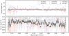 |
Fig. 2 Transmission spectra of HAT-P-41b derived from the five transit observations with OSIRIS R1000R. Upper panel: five individual transmission spectra (colored error bars) and their weighted means (black error bars). Lower panel: same as the upper panel, but zoomed in for clarity. |
Posterior estimates of the central transit time of HAT-P-41b.
4 Atmospheric retrievals
4.1 Model setup
We used the Python package petitRADTRANS (Mollière et al. 2019) to model the transmission spectrum of HAT-P-41b. A one-dimensional isothermal atmosphere was assumed with a pressure range from 10−6 to 102 bar and 100 uniform layers in logarithmic space. We included 12 chemical species (Na, K, MgO, AlO, TiO, VO, MgH, AlH, CaH, CrH, FeH, and H2O) that could show significant spectral features in the OSIRIS wavelength range, and four additional species (NH3, CH4, CO, and CO2) when retrieving the optical-to-near-infrared (NIR) joint transmission spectrum. We assumed free mass fractions mi for each chemical species i and used H2 and He as filler gases to keep the total mass fraction unity with a fixed He/H2 mass ratio of 0.3. Rayleigh-like scattering and collision-induced absorption of H2 and He were also included in the model, with the amplitude of the scattering features multiplied by a factor of As. Additionally, we assumed a uniform opaque cloud cover with a cloud top pressure of Pc, below which all transmitted light would be blocked. The forward model was originally computed with a spectral resolution (λ/∆λ) of 1000 then wavelength binned to the data passbands.
To infer the possible species from the spectral features, we removed one chemical species at a time from the free chemistry model and computed the difference of the log-evidence with and without that species, which is equivalent to the logarithmic Bayes factor. We interpret the Bayes factors using the criteria proposed by Kass & Raftery (1995), where the evidence is strong if |∆ ln 𝒵| ≥ 5, moderate if 3 ≤ |∆ ln 𝒵| < 5, weak if 1 ≤ |∆ ln 𝒵| < 3, and inconclusive if |∆ ln 𝒵| < 1. The Bayesian evidence and posterior estimates were obtained using the nested sampling algorithm in the same way as introduced in Sect. 3.4, but sampled with fewer live points (N = 500) due to the very high computational cost, which still guaranteed ~ 150 000 likelihood evaluations and ~3500 posterior samples.
4.2 OSIRIS transmission spectrum
We first computed the full atmospheric retrieval including all 12 chemical species (Fig. 3). The posterior joint distributions of the atmospheric parameters can be found at ScienceDB4. The retrieved model suggested a clear atmosphere (log10 Pc =  bar) with a temperature of
  , higher than the planetary equilibrium temperature (1941 ± 38 K, Hartman et al. 2012). The Bayesian evidence of the full retrieval (ln 𝒵 = 501.29 ± 0.16) was much stronger than that of a flat model (ln 𝒵 = 402.18 ± 0.12) or a pure scattering model (ln 𝒵 = 467.70 ± 0.14), suggesting significant spectral features in the OSIRIS transmission spectrum. These spectral features can mostly be characterized by the absorption signatures of TiO, while near the blue and red ends some excess absorption could be characterized by the absorption of MgH and CrH, respectively.
We then performed model comparison based on Bayesian evidence to validate the detection of each chemical species. We removed each chemical species from the full retrieval and estimated the Bayesian evidence for a model hypothesis excluding that species. If the new Bayesian evidence is substantially weaker than the Bayesian evidence of the full retrieval, it indicates that the absorption features of the missing species cannot be counteracted by other species, implying the need for that species to characterize the transmission spectrum. According to Table 3, there is very strong evidence for the presence of spectral features of TiO (∆ ln 𝒵 = 21.02), moderate evidence for that of CrH (∆ ln 𝒵 = 3.73), and weak evidence for that of MgH (∆ ln 𝒵 = 2.32) in the OSIRIS transmission spectrum, which can be approximated as a detection significance of 6.8σ for TiO, 3.2σ for CrH, and 2.7σ for MgH (Sellke et al. 2001; Benneke & Seager 2013). We found no evidence for the absorption signatures of the alkali metals or other metal oxides and hydrides.
The absorption features of TiO in the atmosphere of HAT-P-41b have been previously detected by HST STIS measurements (Sheppard et al. 2021), while those of CrH and MgH were discovered for the first time in this work. Sheppard et al. (2021) compared the results of two transmission spectrum models: the equilibrium chemistry models of PLATON and the free chemistry models of AURA. They found suggestive evidence for the optical absorbers and decisive evidence for water vapor in the 0.3–5.0 µm transmission spectrum of HAT-P-41b. While the free chemistry retrieval from AURA supports the presence of absorption features of Na I and AlO in the optical band, the results from PLATON favor the absorption of TiO and VO. However, we did not detect the absorption features of Na I and AlO in the OSIRIS transmission spectrum using the petitRADTRANS free chemistry model. Instead, we observed significantly higher chemical abundances of TiO compared to VO, which is different from the predictions of the equilibrium chemical model. Additionally, we found preliminary evidence for MgH and CrH, which are not included in the equilibrium chemistry model.
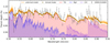 |
Fig. 3 Retrieved transmission spectrum of HAT-P-41b observed with GTC OSIRIS. The error bars are the averaged OSIRIS transmission spectrum. The orange lines are the median and 2σ credible intervals of the posterior models. The black dots are the posterior model after wavelength binning to the observational passbands. The shaded regions below the posterior model indicate the reference models with only TiO (red), MgH (blue), or CrH (purple). |
Bayesian model comparison of the chemical species retrieved with the OSIRIS transmission spectrum.
5 Discussion and conclusion
To precisely constrain the atmospheric chemical abundances, we performed a joint retrieval by combining the OSIRIS transmission spectrum with the 0.3–5.0 µm transmission spectrum presented in Sheppard et al. (2021). To account for possible transit depth offsets due to different instruments and/or light curve analysis methods, three arbitrary offsets were added separately as free parameters with a uniform prior of 𝓤(−1000, 1000) ppm to the HST STIS, HST WFC3 and Spit𝒵er IRAC transmission spectra. As shown in Fig. 4, the retrieved model from the joint transmission spectra exhibits strong absorption signatures of TiO, H2O, and CO2, and tentative signatures of AlO, MgH, and CrH, which are in good agreement with the results from the OSIRIS transmission spectrum in the optical wavelength range.
Figure 5 presents the posterior volume mixing ratios (VMRs5) of each chemical species obtained from the atmospheric retrievals, along with the VMRs predicted by the equilibrium chemistry model computed with GGChem (Woitke et al. 2018) assuming solar abundances. The chemical abundances constrained by the OSIRIS transmission spectrum alone are consistent with those constrained by the joint spectrum, except for AlO and H2O. Based on the joint retrieval, we obtain precise measurements of the abundances of AlO  , TiO
, TiO  , MgH
, MgH  , CrH
, CrH  , H2O
, H2O  , and CO
  . Sheppard et al. (2021) also report the detection of AlO in the optical wavelength range. We note that the main spectral features of AlO are from 0.40 to 0.55 µm and thus the measurement of AlO was mainly from the STIS G430L spectrum rather than the OSIRIS R1000R spectrum. In addition, the low abundances of MgO, VO, CaH, and FeH disfavor the presence of these species in the terminator atmosphere of HAT-P-41b. Comparing the retrieved VMRs with the equilibrium chemistry model that assumes solar abundances, we find super-solar abundances for all the well-constrained chemical species in the joint retrieval (AlO, TiO, MgH, CrH, H2O, and CO2). Although the detections of MgH and CrH were tentative, there is strong evidence for a super-solar TiO abundance (and a super-solar H2O abundance when considering the NIR data), supporting a metal-rich atmosphere for HAT-P-41b.
The high metallicity of the host star ([Fe/H] = 0.21 ± 0.10; Hartman et al. 2012) provides the conditions for the formation of a metal-rich atmosphere for HAT-P-41b. Considering that the equilibrium temperature of HAT-P-41b (Teq = 1941 ± 38 K) is in the empirical transition zone between hot and ultra-hot planets, around 2150 K (Stangret et al. 2022), its atmospheric composition may contain characteristics of both the low-temperature and high-temperature regimes from a statistical point of view. Therefore, aside from the detected H2O, CO2, and refractory molecules, atomic species such as H, Fe, Mg, and alkali metals are also possible to be found in future high-resolution observations of the atmosphere of HAT-P-41b.
The first tentative evidence for CrH was found in the atmosphere of WASP-31b, a hot Jupiter with an equilibrium temperature ~370 K cooler than that of HAT-P-41b, based on the observations of HST STIS G750L (Braam et al. 2021). The presence of CrH in WASP-31b was recently confirmed by highresolution transmission spectroscopy (Flagg et al. 2023). With the addition of HAT-P-41b, which potentially has CrH in its atmosphere, future studies could target the formation of Cr-bearing clouds in its planetary atmosphere (Lodders & Fegley 2006; Morley et al. 2012).
There are other hot Jupiters with temperatures, masses, radii, and host star parameters similar to those of HAT-P-41b, for example, CoRoT-1b (Barge et al. 2008), HAT-P-7b (Pál et al. 2008), HAT-P-32b (Hartman et al. 2011), HAT-P-65b (Hartman et al. 2016), and WASP-19b (Hebb et al. 2010). Observations of these planets show that hot Jupiters with transition-zone equilibrium temperatures orbiting F- to G-type stars can exhibit rich spectral features of both volatile species (e.g., H2O) and refractory species (e.g., TiO) if not obscured by high-altitude clouds or hazes (Huitson et al. 2013; Damiano et al. 2017; Sedaghati et al. 2017, 2021; Tsiaras et al. 2018; Chen et al. 2021; Czesla et al. 2022; Glidic et al. 2022; Changeat et al. 2022; Li et al. 2023; Jiang et al. 2023). The day-night and morning–evening differences could allow H2 and H2O to be dissociated into H− in the hot dayside and evening-side atmospheres, while recombining into water molecules or other metal hydrides in the cooler night-side and morning-side atmospheres (Parmentier et al. 2018). Our preliminary detection of MgH and CrH in the terminator
atmosphere sheds lights on the presence of H− in the hot dayside atmosphere. We speculate that the emission features of the day-side atmosphere might be obscured by the continuum absorption of H−, resulting in an emission spectrum with weak features and thus tending toward an isothermal profile, which would explain why the thermal inversion based on the secondary eclipse measurements from HST and Spit𝒵er was inconclusive (Fu et al. 2022).
In this study, we analyzed the optical transmission spectrum of HAT-P-41b using data from five transits observed by GTC OSIRIS. Our free-chemistry atmospheric retrievals and model comparisons provide strong evidence for the presence of TiO in the atmosphere of HAT-P-41b, and we also tentatively detected the signatures of MgH and CrH. Our joint retrieval analysis, which combined GTC, HST, and Spit𝒵er transmission spectra, yielded results consistent with the analysis of the OSIRIS data and provided precise constraints on the abundances of TiO, MgH, CrH, H2O, and CO2. The detection of abundant optical absorbers in HAT-P-41b’s high-temperature atmosphere suggests the possibility of a thermal inversion in its upper atmosphere. However, current thermal emission spectra have not provided decisive evidence for this inversion (Mansfield et al. 2021; Fu et al. 2022; Changeat et al. 2022), which may be due to the presence of H− obscuring other emission features. Future observations with broader wavelength coverages or higher spectral resolutions, such as those to be obtained by the James Webb Space Telescope (JWST) or other large ground-based telescopes, are needed to further characterize the dayside atmosphere of HAT-P-41b and confirm the signatures of metal hydrides.
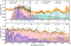 |
Fig. 4 Retrieval results of HAT-P-41b using the optical-to-NIR joint transmission spectra. Upper panel: transmission spectra measured with different instruments, shown as the error bars, where the median instrumental offsets have been applied (−4 ppm for STIS, 758 ppm for G141, and 388 ppm for IRAC). The median and 2σ credible interval of the posterior models are shown as orange lines. The black dots are the median model after wavelength binning. The shaded regions below the posterior model indicate the reference models with only AlO (green), TiO (red), MgH (deep blue), CrH (purple), H2O (sky blue), and CO2 (brown). Lower panel: same as the upper panel, but zoomed into the wavelength range of the OSIRIS transmission spectrum. |
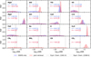 |
Fig. 5 Posterior distributions of the VMRs of chemical species constrained by the OSIRIS transmission spectrum (blue) and the optical-to-NIR joint spectrum (red). The symbol X denotes the median logarithmic VMR (log10 VMR) of the corresponding color. The gray lines indicate the VMRs calculated using GGChem equilibrium chemistry (Woitke et al. 2018) assuming solar abundances at a pressure of 1 bar, where two planetary equilibrium temperatures were considered: 1941 K (dashed, assuming uniform heat redistribution) and 2308 K (dotted, assuming dayside heat redistribution only). |
Acknowledgements
We thank the anonymous referee for their valuable comments and suggestions. G.C. acknowledges the support by the National Natural Science Foundation of China (grant nos. 12122308, 42075122), the B-type Strategic Priority Program of the Chinese Academy of Sciences (grant no. XDB41000000), Youth Innovation Promotion Association CAS (2021315), and the Minor Planet Foundation of the Purple Mountain Observatory. This work is based on observations made with the Gran Telescopio Canarias installed at the Spanish Observatorio del Roque de los Muchachos of the Instituto de Astrofísica de Canarias on the island of La Palma, and on data from the GTC Archive at CAB (CSIC-INTA). The GTC Archive is part of the Spanish Virtual Observatory project funded by MCIN/AEI/10.13039/501100011033 through grant PID2020-112949GB-I00. This work has made use of data from the European Space Agency (ESA) mission Gaia (https://www.cosmos.esa.int/gaia), processed by the Gaia Data Processing and Analysis Consortium (DPAC, https://www.cosmos.esa.int/web/gaia/dpac/consortium). Funding for the DPAC has been provided by national institutions, in particular the institutions participating in the Gaia Multilateral Agreement.
Appendix A Supplementary figures and tables
Observation summary for HAT-P-41b.
Measurements of the HAT-P-41 system and updated constraints on its companion.
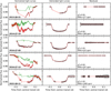 |
Fig. A.1 Fitting results of the broadband transit light curves of HAT-P-41b. Each row corresponds to one transit observation. Left column: Normalized fluxes (black error bars), the best-fit models (red), and the systematic noise (green, also the common-mode systematics). Middle column: Detrended light curves and the best-fit transit models. Right column: Residuals. |
References
- Ambikasaran, S., Foreman-Mackey, D., Greengard, L., Hogg, D. W., & O’Neil, M. 2015, IEEE Trans. Pattern Anal. Mach. Intell., 38, 252 [Google Scholar]
- Barge, P., Baglin, A., Auvergne, M., et al. 2008, A&A, 482, L17 [CrossRef] [EDP Sciences] [Google Scholar]
- Benneke, B., & Seager, S. 2013, ApJ, 778, 153 [Google Scholar]
- Braam, M., van der Tak, F. F. S., Chubb, K. L., & Min, M. 2021, A&A, 646, A17 [NASA ADS] [CrossRef] [EDP Sciences] [Google Scholar]
- Buchner, J., Georgakakis, A., Nandra, K., et al. 2014, A&A, 564, A125 [NASA ADS] [CrossRef] [EDP Sciences] [Google Scholar]
- Burrows, A., Budaj, J., & Hubeny, I. 2008, ApJ, 678, 1436 [Google Scholar]
- Cepa, J., Aguiar, M., Escalera, V. G., et al. 2000, SPIE Conf. Ser., 4008, 623 [Google Scholar]
- Changeat, Q., Edwards, B., Al-Refaie, A. F., et al. 2022, ApJS, 260, 3 [NASA ADS] [CrossRef] [Google Scholar]
- Chen, G., Pallé, E., Parviainen, H., Murgas, F., & Yan, F. 2021, ApJ, 913, L16 [NASA ADS] [CrossRef] [Google Scholar]
- Cutri, R. M., Skrutskie, M. F., van Dyk, S., et al. 2003, VizieR Online Data Catalog: II/246 [Google Scholar]
- Czesla, S., Lampón, M., Sanz-Forcada, J., et al. 2022, A&A, 657, A6 [NASA ADS] [CrossRef] [EDP Sciences] [Google Scholar]
- Damiano, M., Morello, G., Tsiaras, A., Zingales, T., & Tinetti, G. 2017, AJ, 154, 39 [NASA ADS] [CrossRef] [Google Scholar]
- Feroz, F., & Hobson, M. P. 2008, MNRAS, 384, 449 [NASA ADS] [CrossRef] [Google Scholar]
- Feroz, F., Hobson, M. P., & Bridges, M. 2009, MNRAS, 398, 1601 [NASA ADS] [CrossRef] [Google Scholar]
- Flagg, L., Turner, J. D., Deibert, E., et al. 2023, ApJ, 953, L19 [NASA ADS] [CrossRef] [Google Scholar]
- Fortney, J. J., Lodders, K., Marley, M. S., & Freedman, R. S. 2008, ApJ, 678, 1419 [CrossRef] [Google Scholar]
- Fortney, J. J., Shabram, M., Showman, A. P., et al. 2010, ApJ, 709, 1396 [NASA ADS] [CrossRef] [Google Scholar]
- Fu, G., Sing, D. K., Deming, D., et al. 2022, AJ, 163, 190 [NASA ADS] [CrossRef] [Google Scholar]
- Gaia Collaboration (Prusti, T., et al.) 2016, A&A, 595, A1 [NASA ADS] [CrossRef] [EDP Sciences] [Google Scholar]
- Gaia Collaboration (Vallenari, A., et al.) 2023, A&A, 674, A1 [NASA ADS] [CrossRef] [EDP Sciences] [Google Scholar]
- Gibson, N. P., Aigrain, S., Barstow, J. K., et al. 2013, MNRAS, 428, 3680 [Google Scholar]
- Glidic, K., Schlawin, E., Wiser, L., et al. 2022, AJ, 164, 19 [NASA ADS] [CrossRef] [Google Scholar]
- Guillot, T. 2010, A&A, 520, A27 [NASA ADS] [CrossRef] [EDP Sciences] [Google Scholar]
- Hartman, J. D., Bakos, G. Á., Torres, G., et al. 2011, ApJ, 742, 59 [NASA ADS] [CrossRef] [Google Scholar]
- Hartman, J. D., Bakos, G. Á., Béky, B., et al. 2012, AJ, 144, 139 [NASA ADS] [CrossRef] [Google Scholar]
- Hartman, J. D., Bakos, G. Á., Bhatti, W., et al. 2016, AJ, 152, 182 [NASA ADS] [CrossRef] [Google Scholar]
- Hebb, L., Collier-Cameron, A., Triaud, A. H. M. J., et al. 2010, ApJ, 708, 224 [NASA ADS] [CrossRef] [Google Scholar]
- Huitson, C. M., Sing, D. K., Pont, F., et al. 2013, MNRAS, 434, 3252 [NASA ADS] [CrossRef] [Google Scholar]
- Husser, T. O., Wende-von Berg, S., Dreizler, S., et al. 2013, A&A, 553, A6 [NASA ADS] [CrossRef] [EDP Sciences] [Google Scholar]
- Jiang, C., Chen, G., Pallé, E., et al. 2022, A&A, 664, A50 [NASA ADS] [CrossRef] [EDP Sciences] [Google Scholar]
- Jiang, C., Chen, G., Pallé, E., et al. 2023, A&A, 675, A62 [NASA ADS] [CrossRef] [EDP Sciences] [Google Scholar]
- Kass, R. E., & Raftery, A. E. 1995, J. Am. Stat. Assoc., 90, 773 [Google Scholar]
- Lewis, N. K., Wakeford, H. R., MacDonald, R. J., et al. 2020, ApJ, 902, L19 [NASA ADS] [CrossRef] [Google Scholar]
- Li, X.-K., Chen, G., Zhao, H.-B., & Wang, H.-C. 2023, Res. Astron. Astrophys., 23, 025018 [NASA ADS] [CrossRef] [Google Scholar]
- Lodders, K., & Fegley, B., J. 2006, in Astrophysics Update 2, ed. J. W. Mason, 1 [Google Scholar]
- Mansfield, M., Line, M. R., Bean, J. L., et al. 2021, Nat. Astron., 5, 1224 [CrossRef] [Google Scholar]
- Mollière, P., Wardenier, J. P., van Boekel, R., et al. 2019, A&A, 627, A67 [Google Scholar]
- Morley, C. V., Fortney, J. J., Marley, M. S., et al. 2012, ApJ, 756, 172 [NASA ADS] [CrossRef] [Google Scholar]
- Nortmann, L., Pallé, E., Murgas, F., et al. 2016, A&A, 594, A65 [NASA ADS] [CrossRef] [EDP Sciences] [Google Scholar]
- Pál, A., Bakos, G. Á., Torres, G., et al. 2008, ApJ, 680, 1450 [CrossRef] [Google Scholar]
- Parmentier, V., Line, M. R., Bean, J. L., et al. 2018, A&A, 617, A110 [NASA ADS] [CrossRef] [EDP Sciences] [Google Scholar]
- Parviainen, H. 2015, MNRAS, 450, 3233 [Google Scholar]
- Parviainen, H., & Aigrain, S. 2015, MNRAS, 453, 3821 [Google Scholar]
- Seager, S., & Sasselov, D. D. 2000, ApJ, 537, 916 [Google Scholar]
- Sedaghati, E., Boffin, H. M. J., MacDonald, R. J., et al. 2017, Nature, 549, 238 [Google Scholar]
- Sedaghati, E., MacDonald, R. J., Casasayas-Barris, N., et al. 2021, MNRAS, 505, 435 [NASA ADS] [CrossRef] [Google Scholar]
- Sellke, T., Bayarri, M. J., & Berger, J. O. 2001, Am. Statist., 55, 62 [Google Scholar]
- Sharp, C. M., & Burrows, A. 2007, ApJS, 168, 140 [NASA ADS] [CrossRef] [Google Scholar]
- Sheppard, K. B., Welbanks, L., Mandell, A. M., et al. 2021, AJ, 161, 51 [NASA ADS] [CrossRef] [Google Scholar]
- Stangret, M., Casasayas-Barris, N., Pallé, E., et al. 2022, A&A, 662, A101 [NASA ADS] [CrossRef] [EDP Sciences] [Google Scholar]
- Tsiaras, A., Waldmann, I. P., Zingales, T., et al. 2018, AJ, 155, 156 [NASA ADS] [CrossRef] [Google Scholar]
- Wakeford, H. R., Sing, D. K., Stevenson, K. B., et al. 2020, AJ, 159, 204 [Google Scholar]
- Welbanks, L., McGill, P., Line, M., & Madhusudhan, N. 2023, AJ, 165, 112 [NASA ADS] [CrossRef] [Google Scholar]
- Woitke, P., Helling, C., Hunter, G. H., et al. 2018, A&A, 614, A1 [NASA ADS] [CrossRef] [EDP Sciences] [Google Scholar]
- Wöllert, M., Brandner, W., Bergfors, C., & Henning, T. 2015, A&A, 575, A23 [NASA ADS] [CrossRef] [EDP Sciences] [Google Scholar]
Measured with the full width at half maximum of the stellar PSF fitted by a Gaussian function along the spatial direction at the central wavelength of ~750 nm.
Measured with the pixel drift of the stellar PSF fitted by a Gaussian function along the spatial direction at the central wavelength of ~750 nm.
Volume mixing ratio VMR = mi ⋅ µ/µi, where mi and µi are the mass fraction and the particle mass of the species i, and µ is the atmospheric mean molecular weight.
All Tables
Bayesian model comparison of the chemical species retrieved with the OSIRIS transmission spectrum.
All Figures
|
Fig. 1 Narrowband flux ratios between the companion and HAT-P-41. The error bars are the observed flux ratios, and the orange line is the best-fit curve obtained using the PHOENIX model spectra. |
| In the text | |
|
Fig. 2 Transmission spectra of HAT-P-41b derived from the five transit observations with OSIRIS R1000R. Upper panel: five individual transmission spectra (colored error bars) and their weighted means (black error bars). Lower panel: same as the upper panel, but zoomed in for clarity. |
| In the text | |
|
Fig. 3 Retrieved transmission spectrum of HAT-P-41b observed with GTC OSIRIS. The error bars are the averaged OSIRIS transmission spectrum. The orange lines are the median and 2σ credible intervals of the posterior models. The black dots are the posterior model after wavelength binning to the observational passbands. The shaded regions below the posterior model indicate the reference models with only TiO (red), MgH (blue), or CrH (purple). |
| In the text | |
|
Fig. 4 Retrieval results of HAT-P-41b using the optical-to-NIR joint transmission spectra. Upper panel: transmission spectra measured with different instruments, shown as the error bars, where the median instrumental offsets have been applied (−4 ppm for STIS, 758 ppm for G141, and 388 ppm for IRAC). The median and 2σ credible interval of the posterior models are shown as orange lines. The black dots are the median model after wavelength binning. The shaded regions below the posterior model indicate the reference models with only AlO (green), TiO (red), MgH (deep blue), CrH (purple), H2O (sky blue), and CO2 (brown). Lower panel: same as the upper panel, but zoomed into the wavelength range of the OSIRIS transmission spectrum. |
| In the text | |
|
Fig. 5 Posterior distributions of the VMRs of chemical species constrained by the OSIRIS transmission spectrum (blue) and the optical-to-NIR joint spectrum (red). The symbol X denotes the median logarithmic VMR (log10 VMR) of the corresponding color. The gray lines indicate the VMRs calculated using GGChem equilibrium chemistry (Woitke et al. 2018) assuming solar abundances at a pressure of 1 bar, where two planetary equilibrium temperatures were considered: 1941 K (dashed, assuming uniform heat redistribution) and 2308 K (dotted, assuming dayside heat redistribution only). |
| In the text | |
|
Fig. A.1 Fitting results of the broadband transit light curves of HAT-P-41b. Each row corresponds to one transit observation. Left column: Normalized fluxes (black error bars), the best-fit models (red), and the systematic noise (green, also the common-mode systematics). Middle column: Detrended light curves and the best-fit transit models. Right column: Residuals. |
| In the text | |
Current usage metrics show cumulative count of Article Views (full-text article views including HTML views, PDF and ePub downloads, according to the available data) and Abstracts Views on Vision4Press platform.
Data correspond to usage on the plateform after 2015. The current usage metrics is available 48-96 hours after online publication and is updated daily on week days.
Initial download of the metrics may take a while.