| Issue |
A&A
Volume 687, July 2024
|
|
|---|---|---|
| Article Number | A9 | |
| Number of page(s) | 10 | |
| Section | Planets and planetary systems | |
| DOI | https://doi.org/10.1051/0004-6361/202449915 | |
| Published online | 25 June 2024 | |
Detection of Na in the atmosphere of the hot Jupiter HAT-P-55b
1
CAS Key Laboratory of Planetary Sciences, Purple Mountain Observatory, Chinese Academy of Sciences,
No. 10 Yuanhua Road, Qixia District,
210023
Nanjing,
PR China
e-mail: guochen@pmo.ac.cn
2
School of Astronomy and Space Science, University of Science and Technology of China,
No. 96 Jinzhai Road, Baohe District,
230026
Hefei,
PR China
3
CAS Center for Excellence in Comparative Planetology,
No. 96 Jinzhai Road, Baohe District,
230026
Hefei,
PR China
4
Instituto de Astrofísica de Canarias (IAC),
Vía Láctea s/n,
38205 La
Laguna,
Tenerife,
Spain
5
Departamento de Astrofísica, Universidad de La Laguna (ULL),
C/ Padre Herrera,
38206 La
Laguna,
Tenerife,
Spain
6
Komaba Institute for Science, The University of Tokyo,
3-8-1 Komaba, Meguro,
Tokyo
153-8902,
Japan
7
Astrobiology Center,
2-21-1 Osawa, Mitaka,
Tokyo
181-8588,
Japan
Received:
9
March
2024
Accepted:
21
April
2024
The spectral signatures of optical absorbers, when combined with those of infrared molecules, play a critical role in constraining the cloud properties of exoplanet atmospheres. We aim to use optical transmission spectroscopy to confirm the tentative color signature previously observed by multiband photometry in the atmosphere of hot Jupiter HAT-P-55b. We observed a transit of the HAT-P-55b with the OSIRIS spectrograph on the Gran Telescopio Canarias (GTC). We created two sets of spectroscopic light curves, using the conventional band-integrated method and the newly proposed pixel-based method, to derive the transmission spectrum. We performed Bayesian spectral retrieval analyses on the transmission spectrum to interpret the observed atmospheric properties. The transmission spectra derived from the two methods are consistent, both spectrally resolving the tentative color signature observed by MuSCAT2. The retrievals on the combined OSIRIS and MuSCAT2 transmission spectrum yield a detection of Na at 5.5σ and a tentative detection of MgH at 3.4σ. The current optical-only wavelength coverage cannot constrain the absolute abundances of the atmospheric species. Space-based observations covering the molecular infrared bands or ground-based high-resolution spectroscopy are needed to further constrain the atmospheric properties of HAT-P-55b.
Key words: methods: data analysis / techniques: spectroscopic / planets and satellites: atmospheres / planets and satellites: individual: HAT-P-55b
© The Authors 2024
 Open Access article, published by EDP Sciences, under the terms of the Creative Commons Attribution License (https://creativecommons.org/licenses/by/4.0), which permits unrestricted use, distribution, and reproduction in any medium, provided the original work is properly cited.
This article is published in open access under the Subscribe to Open model. Subscribe to A&A to support open access publication.
1 Introduction
The atmospheres of hot Jupiters can provide us with hints of the planet’s formation history through atmospheric properties such as metallicity and elemental ratios (e.g., Öberg et al. 2011; Madhusudhan et al. 2014; Mordasini et al. 2016; Lothringer et al. 2021). Among the various observational techniques that can constrain these atmospheric properties, transmission spec-troscopy (Seager & Sasselov 2000) has been the most widely used, performed on dozens of exoplanets to study the absorption and scattering signatures present in the atmosphere at the day-night terminator. Retrieval methods (e.g., Madhusudhan & Seager 2009) can extract the atmospheric properties from observed spectra based on certain assumed parametric forward atmospheric models.
However, the atmospheric retrieval of transmission spectra could suffer from potential degeneracies (Lecavelier Des Etangs et al. 2008; Benneke & Seager 2012; de Wit & Seager 2013; Griffith 2014; Bétrémieux & Swain 2017; Heng & Kitzmann 2017), such as the degeneracy between chemical abundances and cloud properties, if the observations were made in a limited spectral range. Welbanks & Madhusudhan (2019) show that including optical wavelengths, which are sensitive to clouds and hazes, along with infrared wavelengths can mitigate the degeneracy between chemical abundances and cloud properties. On the other hand, to accurately constrain the properties of clouds and hazes, it is necessary to rely on the detection and characterization of specific spectral features (Jiang et al. 2023).
In particular, Na and K, the dominant optical opacity sources of typical hot Jupiters (Fortney et al. 2010), can exhibit pressure-broadened line profiles depending on the cloudiness of the atmosphere, and these profiles play a critical role in tightly constraining molecular abundances (e.g., Welbanks et al. 2019; Chen et al. 2022). Recent low-resolution ground- and space-based transmission spectroscopy surveys (e.g., Sing et al. 2011; Chen et al. 2017b, 2018, 2020, 2022; Nikolov et al. 2018; Pearson et al. 2019; Ahrer et al. 2022; Feinstein et al. 2023) have begun to manifest the line profile of Na and K with tens of nearly uniform narrow bands (≤10 nm), laying the basis for improved future atmospheric retrievals from the optical to the infrared.
Here we present a follow-up transit observation carried out to obtain the transmission spectrum of the hot Jupiter HAT-P-55b using the Optical System for Imaging and low-Intermediate-Resolution Integrated Spectroscopy (OSIRIS; Cepa et al. 2000) mounted on the 10.4 m Gran Telescopio Canarias (GTC). HAT-P-55b is a hot Jupiter orbiting a Sun-like star discovered by Juncher et al. (2015). Based on four transits observed with the MuSCAT2 (Multicolor Simultaneous Camera for studying Atmospheres of Transiting exoplanets 2) four-color simultaneous camera on the 1.52 m Telescopio Carlos Sánchez (TCS), Kang et al. (2024) improved the estimate of the transit and physical parameters for the HAT-P-55 system, obtaining a radius of  , a mass of
  , and an equilibrium temperature of 1367 ± 11 K. The derived MuSCAT2 broadband transmission spectrum in the g, r, i, and zs was not completely flat, showing moderate evidence that the observed variations originate from the planetary atmosphere. The goal of this study is to use GTC/OSIRIS to spectrally resolve the optical absorbers responsible for the MuSCAT2 transit depth color variations.
This paper is organized as follows. In Sect. 2, we summarize the details of the transit observation and data reduction. In Sect. 3, we describe the light curve analysis and propose a new pixel-based approach to deriving the transmission spectrum in addition to the conventional band-integrated method. In Sect. 4, we present the derived transmission spectrum and perform Bayesian spectral retrieval analysis on the available transmission spectra to understand the atmospheric properties. Finally, we draw conclusions and present our discussion in Sect. 5.
2 Observations and data reduction
A transit event of the hot Jupiter HAT-P-55b was observed with GTC OSIRIS on May 2, 2020 from 00:23 UT to 05:41 UT. For the transit observation, OSIRIS was configured in the long-slit spectroscopic mode with a 40″ wide slit and the R1000R grism to cover a wavelength range of 510 to 1000 nm. The OSIRIS CCDs were read in 200 kHz readout mode with 2 × 2 pixel binning. Each binned pixel has a spatial scale of 0.254″ and an average instrumental dispersion of 0.26 nm. The time series consists of single exposures of 30 s. During the observation the sky was mostly clear and the seeing varied between 0.7″ and 1.9″. The details of the observation are summarized in Table 1.
To calibrate the flux of HAT-P-55, a reference star (2MASS J17371483+2543127) was simultaneously observed in the same slit. The target and reference stars, which have r-band magnitudes of 13.060 and 12.926, respectively (Zacharias et al. 2015), were placed on the same CCD at a distance of 2.18′. For wavelength calibration, the HeAr, Ne, and Xe arc lamps were measured through the 1.00″ wide slit using the same R1000R grism.
The raw OSIRIS spectral images were reduced using the approaches developed in our previous studies (e.g., Chen et al. 2017a, 2018, 2020; Jiang et al. 2022), including calibration of overscan, bias, flat field, cosmic rays, and sky background. In particular, the sky background model was constructed in the wavelength domain based on the two-dimensional pixel-to-wavelength solution derived from the arc lamps. The one-dimensional spectra of the target and reference stars were extracted using the optimal extraction algorithm (Horne 1986) with an aperture diameter of 42 pixels, optimized to minimize subsequent light curve scatter, and aligned to the laboratory rest frame. The center of the exposure time in UT was calculated for each spectrum and converted to barycentric Julian dates in barycentric dynamical time (BJDTDB; Eastman et al. 2010), which were recorded as time stamps.
Two methods were used to create the light curves. Since the pixel-to-wavelength transformation solution is nonlinear, the flux within a given passband can be obtained either in the original pixel grid or in the linearly resampled wavelength grid. In our conventional method (Chen et al. 2017a), to eliminate the interpolation process, the pixel range for a given passband was calculated and only the flux of the partial pixels at the edge was interpolated, while those of the full pixels were summed directly. Two types of light curves were created. For the band-integrated white light curve, the flux was summed within the wavelength range of 511.5–901.5 nm, excluding 754–768 nm due to the steep absorption feature of the telluric oxygen A-band. The wavelengths longer than 901.5 nm were not used to avoid potential second-order contamination and fringing effects. For the band-integrated spectroscopic light curves, the entire wavelength range was divided into 55 passbands of 5 nm, 1 passband of 15 nm, and 3 passband of 30 nm. Each light curve was normalized by its own out-of-transit flux.
In addition to the conventional method, we introduced a new method for creating the spectroscopic light curves. The band-integrated white light curve in our new method was the same as in the conventional method. However, the spectroscopic light curves were created in a different way. The flux of the original pixels in each spectrum does not form a valid time series due to misalignment along the time axis and nonlinear wavelength solutions. Therefore, all spectra were resampled using the misalignment corrected wavelength solutions in a linear wavelength grid from 511.5 to 901.5 nm with an average dispersion of 0.26 nm per pixel, taking into account flux conservation. This resulted in 1500 uniform pseudo pixels and thus 1500 pixel light curves. The transit depths derived from the spectroscopic light curves using these two methods are compared in the subsequent analysis.
Details of the transit observation for HAT-P-55b.
3 Light curve analysis
3.1 White light curve
The white light curve was modeled with a transit model configured with the nonlinear limb darkening law and a circular orbit (Juncher et al. 2015) using the Python package batman (Kreidberg 2015). The transit model was parameterized by orbital period (P), radius ratio (Rp/R★), orbital inclination (i), scaled semimajor axis (a/R★), mid-transit time (Tmid), and four limb darkening coefficients (LDCs; ui). The values of P, i, and a/R★ were fixed to 3.58523130 days, 86.80°, and 9.06, respectively, derived in Kang et al. (2024). The four LDCs were fixed to the precalculated values (u1 = 1.2247, u2 = −2.0154, u3 = 2.6623, u4 = −1.0898) from the PHOENIX stellar atmosphere models using the Python code of Espinoza & Jordán (2015), with stellar effective temperature Teff = 5800 K, surface gravity log g★ = 4.5, and metallicity [Fe/H] = 0.0.
The correlated systematics in the light curve were described by Gaussian processes (GPs; e.g., Gibson et al. 2012), assuming the transit model as the mean function. The Python package george (Ambikasaran et al. 2015) was used to perform the GP regression with the capability of multidimensional inputs in the covariance matrix, which adopted the Matern-3/2 kernel  for two points in each input at a given radius r. The kernel was a multiplication of the kernels of each individual input, and the inputs to the combined kernel were the time (t), spectral drift (x), spatial drift (y), full width at half maximum of the target point spread function (s), and rotation angle (θ). The combined kernel had a scale length hyperparam-eter ρi for each input and a single covariance hyperparameter
  . An additional white noise jitter
  was used to account for potential underestimation of white noise.
To investigate the posterior probability distributions of the free parameters, the affine invariant Markov chain Monte Carlo (MCMC) ensemble sampler was implemented using the Python package emcee (Foreman-Mackey et al. 2013). Uniform priors were used for Tmid and log-uniform priors for the GP hyperpa-rameters. Given the presence of strong correlated noise distorting the white light curve, a normal prior of 0.1220 ± 0.0007 from Kang et al. (2024) was imposed on Rp/R★ to better constrain the correlated systematics, useful for extracting the common mode trend. For the MCMC process, two short chains were run for the burn-in phase and one long chain to ensure convergence for the posterior estimation.
Table 2 gives a summary of the assumed priors and estimated posteriors for the parameters used in the modeling of the white light curve. Figure 1 shows the white light curve and the best-fit model. The best-fit light curve residuals have a standard derivation of 289 ppm, which is 1.94 times the expected photon noise.
Parameters derived from the white light curve.
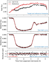 |
Fig. 1 Band-integrated white light curve of HAT-P-55 observed with GTC/OSIRIS. First row: flux time series of HAT-P-55 and its reference star. Second row: raw light curve after dividing the flux of HAT-P-55 by that of the reference. The red line represents the best-fit combined transit and systematics model. Third row: light curve after removal of the systematics. Fourth row: Best-fit light curve residuals. |
3.2 Spectroscopic light curves
Two sets of spectroscopic light curves were produced using the conventional method and the new methods described in Sect. 2. Similar to the correlated systematics in the white light curve, there was a common mode trend in the spectroscopic light curves. An empirical model for the common mode trend was derived by dividing the raw white light curve by its best-fit transit model. For the products of both methods, each individual spectroscopic light curve was divided by this empirical model to correct for the common mode systematics before further analysis.
For the conventional method, the 59 band-integrated spectro-scopic curves were modeled in the same way as the white light curve, with the same Matern-3/2 kernel and the same GP inputs, except that the mid-transit time was fixed to the one derived in the white light curve (see Table 2) and the radius ratios were fitted with uniform priors 𝒰(0.07, 0.17).
For the new method, the 1500 pixel light curves were also modeled with freely fitted radius ratios with uniform priors and the same fixed mid-transit time. However, unlike the band-integrated spectroscopic light curves, the pixel light curves were dominated by white noise instead of correlated noise. To avoid poor constraints on the GP hyperparameters in the case of high-dimensional GP inputs, only the time vector was used in the covariance kernel of the GP regression of the pixel light curves. In addition, to reduce computational cost, the Python package celerite (Foreman-Mackey et al. 2017) was used to perform the GP regression with an approximated Matern-3/2 kernel. To improve the signal-to-noise ratio, the transit depths of the pixel light curves were binned into the 59 passbands used in the conventional method.
Table 3 presents the chromatic radius ratios (i.e., the transmission spectra) derived from the spectroscopic light curves produced by the conventional method and the new method, along with the adopted nonlinear LDCs. Figure 2 shows the matrix of the pixel-by-pixel spectroscopic light curves using the new method along with the best-fit light curve residuals. In general, a light curve precision of 0.76–2.12 times the expected photon noise is achieved when modeling pixel light curves, which is in broad agreement with the range of 1.33–2.07 obtained in conventional band-integrated spectroscopic light curves.
Transmission spectra of HAT-P-55b obtained via the conventional method and the new method.
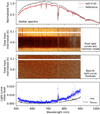 |
Fig. 2 Pixel-by-pixel spectroscopic light curves of HAT-P-55 observed with GTC/OSIRIS. First row: spectra of HAT-P-55 and the reference star. Second row: matrix of pixel light curves after removal of the common mode systematics. Third row: matrix of the best-fit light curve residuals. Fourth row: rms of each pixel light curve, compared to the expected photon noise. |
4 Results and interpretations
4.1 Transmission spectrum
As shown in Fig. 3, the GTC/OSIRIS transmission spectra derived from the conventional and new methods have a difference with a chi-squared value of χ2 = 34.2 for 59 degrees of freedom, indicating good agreement between the two methods. Allowing a free offset (ΔRp/R★ = 0.00094 ± 0.00027) between them would reduce the difference to a chi-squared value of χ2 = 22.6 for 58 degrees of freedom. The largest deviation is measured at 764 nm, which is heavily contaminated by the telluric oxygen A-band. The main difference between the two methods is that the conventional method produces flux-weighted radius ratios and systematics in each spectroscopic band, while the new method derives radius ratios on a pixel basis and then calculates the average values of all pixels in the corresponding band without weighting. However, the two methods resulted in consistent transmission spectra in this work.
In the following analysis, we focus on the transmission spectrum derived from the new method, excluding the telluric-contaminated bands at 759 nm and 764 nm. This OSIRIS spectrum is significantly not flat at a confidence level of 8.7σ (χ2 = 201.8 for 56 degrees of freedom). For comparison, the broadband transmission spectrum obtained by Kang et al. (2024) using TCS/MuSCAT2 is also shown in Fig. 3. The OSIRIS and MuSCAT2 transmission spectra show a similar spectral shape: the radius ratio increases toward 589 nm but decreases for wavelengths longer than 589 nm. This implies that the potential atmospheric spectral signature observed in the MuSCAT2 broadband “spectrum” could be due to the Na absorption, as suggested by the resolved spectral shape of the OSIRIS spectrum.
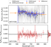 |
Fig. 3 Comparison of HAT-P-55b’s transmission spectra. Upper panel: transmission spectra of HAT-P-55b. The blue triangles and black circles show the OSIRIS transmission spectra obtained with the conventional (“band”) and new (“pixel-binned”) methods. The gray dots show the pixel transmission spectrum. The orange squares show the broadband transmission spectrum obtained with MuSCAT2 by Kang et al. (2024). Bottom panel: difference between the new and conventional methods (red diamonds) and the corresponding histogram. The dashed line marks an overall offset of ΔRp/R★ = −0.00094. |
4.2 Atmospheric retrievals
4.2.1 Model setup
To interpret the combined OSIRIS and MuSCAT2 transmission spectra of HAT-P-55b, we performed spectral retrieval analyses on the observed spectra. We used the Python package petitRADTRANS (Mollière et al. 2019) to create forward models for the planetary atmosphere in the transmission geometry, and the Python package PyMultiNest (Buchner et al. 2014) to estimate model evidence and parameter posterior distributions in the Bayesian framework using the nested sampling algorithm.
In our models, we assumed an isothermal atmosphere with a temperature of Tiso and divided the pressure range between 102 and 10−6 bar into 100 equally spaced layers in logarithmic space. We set the reference pressure P0 as a free parameter, corresponding to the white-light planetary radius (Rp = 1.324 RJ). We used the planetary gravity log gp = 2.926 and the stellar radius R★ = 1.105 R⊙ to compute the transmission spectra in terms of planet-to-star radius ratio. The values of the planetary and stellar parameters were taken from Kang et al. (2024). Our models included line opacity sources from gas species as well as continuum opacity sources from Rayleigh scattering and collision-induced absorption of H2 and He. Following the cloud prescription of MacDonald & Madhusudhan (2017), we assumed that the planetary atmosphere consisted of two equivalent components, a cloudless sector and a cloudy sector with a cloud fraction of ø. In the cloudy sector, clouds and hazes were parameterized by the cloud top pressure Pcloud and the enhancement factor ARS over nominal gas Rayleigh scattering, respectively.
We used two approaches to treat the line opacities in addition to the filler gases H2 and He. In the first approach, we assumed that the atmospheric species were in chemical equilibrium. We adopted the precalculated chemical equilibrium grid provided in the poor_mans_nonequ_chem sub-package of petitRADTRANS, where the following 14 species are available for use: Na, K, TiO, VO, H2O, FeH, CH4, CO, CO2, HCN, C2H2, H2S, SiO, NH3, and PH3. We interpolated the mass mixing ratio Xi of the species i in the grid using the carbon-to-oxygen number ratio (C/O) and the metallicity Z along with the temperature-pressure profile.
In the second approach, we imposed no chemical constraints on the atmospheric species. For the list of species in the first approach, we kept only those with significant spectral signatures in the wavelength range covered by the OSIRIS and MuSCAT2 data. We also added a few metal hydrides with optical spectral band heads observable in the atmospheres of brown dwarfs (Visscher et al. 2010). This results in ten species in use: Na, K, TiO, VO, H2O, FeH, CaH, CrH, MgH, and AlH. For each species, the mass mixing ratio Xi was a free parameter and constant over the calculated pressure range, free from any chemical consideration. The filler gases H2 and He had a mass mixing ratio of 3:1.
On the data side, we used a free offset ΔGTC for the OSIRIS spectrum to eliminate possible systematic offsets introduced by different instruments. Uniform or log-uniform priors were adopted for all the free parameters, as listed in Table 4. To perform model comparisons for the spectral retrievals, we computed the Bayes factor  for the a and b models. Following Trotta (2008) and Benneke & Seager (2013), we adopted the ln
  values of 1.0, 2.5, and 5.0 as starting points for “weak,” “moderate,” and “strong” evidence in favor of the a-model over the b-model; we also converted the Bayes factor to approximately frequentist significance values.
4.2.2 Retrieval results
The retrieved models and parameters of our two assumptions are shown in Figs. 4 and 5 and Table 4. Table 5 presents the Bayesian model comparison for the retrievals assuming free chemistry.
Our retrieval analyses begin with the assumption of equilibrium chemistry. The combined OSIRIS and MuSCAT2 data can tightly constrain the reference pressure to  bar and the instrumental offset to
  ppm. The retrieved cloud top pressure of
  bar indicates that the clouds are relatively deep in the cloudy sector, while the scattering enhancement of
  is consistent with gas Rayleigh scattering, which together could cause the unconstrained cloud fraction of
  . The retrieved atmospheric temperature
  K is strongly skewed toward the upper boundary of the prior, much higher than the equilibrium temperature 1367 ± 11 K (Kang et al. 2024). Our equilibrium chemistry retrieval also shows that the atmosphere of HAT-P-55b has a metallicity of
  solar and a high C/O ratio of
  . Accordingly, the oxide molecules such as H2O, TiO, and VO are deficient, and Na absorption with a prominent pressure broadening is the dominant opacity source.
Our free chemistry retrievals are used to explore which species might be responsible for the observed spectral signatures. The full free chemistry model yielded an atmospheric temperature of  K, a cloud top pressure of
  bar, a scattering enhancement of
  , and a cloud fraction of
  , consistent with those in the equilibrium chemistry assumption. The only significant deviation comes from the retrieved reference pressure, which drops to
  mbar in the free chemistry assumption. Of the 10 species included, only the mass mixing ratios of Na and MgH are constrained,
  and
and  dex, while those of H2O and AlH are unconstrained. For the rest, 3σ upper limits of <–3.11 dex are obtained for K, <–7.11 dex for TiO, <–6.66 dex for VO, <–3.27 for FeH, <–8.22 dex for CaH, and <–3.90 dex for CrH.
However, these mass mixing ratios in the free chemistry retrieval, as well as the metallicity in the equilibrium chemistry retrieval, may be biased because the current wavelengths covered by OSIRIS and MuSCAT2 are limited to optical, which has poor coverage of the major molecules contributing to metallicity and C/O (e.g., H2O, CO, CO2, and CH4). The relative difference between optical absorbers and infrared molecules is crucial for constraining reference pressure and chemical abundances (Welbanks & Madhusudhan 2019). Indeed, strong anticorre-lations are found between reference pressure and metallicity, between reference pressure and mass mixing ratios, and between reference pressure and instrumental offset. On the other hand, the mass mixing ratios of Na and MgH are strongly correlated. Given these degeneracies, which could only be mitigated by future follow-up observations in the infrared, relative abundances are more reliable. The relative mass mixing ratio between MgH and Na measured in the free chemistry retrieval, log XMgH/XNa =  dex, is consistent with the prediction of equilibrium chemistry with solar composition (–2.80 dex).
The free chemistry retrieval was repeated after removing each of the 10 species, and the model evidence was compared to that of the full free chemistry model to assess the contribution of that species. As a result, Na is strongly favored with  and MgH is moderately favored with
  . In contrast, CaH is moderately disfavored
  , while TiO
  and VO
  are weakly disfavored.
To confirm whether the combinations of other species could mimic the observed broad spectral profile provided by Na, we performed additional retrieval tests on a more extensive list of species with potential spectral signatures within 510–700 nm, including Na, K, TiO, VO, H2O, FeH, CaH, CrH, MgH, AlH, H2S, HCN, NH3, AlO, Fe, Li, Ti, and V. The results still strongly favor the presence of Na with  , ruling out the possibility of compensating for the absence of Na absorption by combinations of other species.
To assess whether the Na detection was driven by specific data points, we also performed additional retrieval tests by masking some passbands of the OSIRIS transmission spectrum. Masking the 589 nm passband would lead to Na detection with  , while masking three data points (584 nm, 589 nm, 594 nm) reduces the significance to
  . This indicates that the current inference of Na detection is driven not only by the few data points at the line core of Na, but also by its very broad line wing.
Parameter estimation for spectral retrievals.
Bayesian model comparison for the free chemistry retrievals.
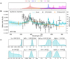 |
Fig. 4 Retrieval analysis of the transmission spectra of HAT-P-55b assuming equilibrium chemistry. Panel a: main species contributing to the spectral signatures. Panel b: transmission spectra obtained with GTC/OSIRIS and TCS/MuSCAT2, along with the median, 1σ, and 2σ confidence levels of the retrieved models. Panel c: posterior distributions of the free parameters in the assumed atmospheric model. |
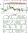 |
Fig. 5 Retrieval analysis of the transmission spectra of HAT-P-55b assuming free chemistry. Panel a: main species contributing to the spectral signatures. Panel b: transmission spectra obtained with GTC/OSIRIS and TCS/MuSCAT2, along with the median, 1σ, and 2σ confidence levels of the retrieved models. Panel c: posterior distributions of the free parameters in the assumed atmospheric model. |
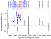 |
Fig. 6 Equivalent width of Na measured in low-resolution transmission spectra for planets with reported Na detection. Measurements with a S/N greater than 2 are shown as filled circles, and the others are shown as empty circles. HAT-P-55b is highlighted in red. |
5 Conclusions and discussion
We have conducted a follow-up spectrophotometric transit observation of the hot Jupiter HAT-P-55b using GTC/OSIRIS. We derived transmission spectra for this planet using the conventional band-integrated method and the new pixel-based method; these spectra are consistent with each other and in broad agreement with the tentative color signature previously observed by Kang et al. (2024) using TCS/MuSCAT2. We performed Bayesian spectral retrieval analyses on the combined OSIRIS and MuSCAT2 transmission spectrum and find that the observed spectral signature is likely due to Na and possibly partially from MgH. While it is difficult to constrain the absolute abundances of Na and MgH with the current optical-only wavelength coverage, the relative mass mixing ratio between Na and MgH is consistent with the prediction of the solar composition at chemical equilibrium.
The prominent broad Na absorption signature makes HAT-P-55b a new addition to the small group of known hot Jupiters that exhibit potential alkali pressure broadening. Following the line broadening metric proposed by Chen et al. (2020) but without normalization, we calculated the equivalent width within an 80 nm band centered on the Na line in low-resolution transmission spectra for planets with Na detection reported in the literature. As shown in Fig. 6 and Table 6, nine planets have large positive equivalent widths for Na with S/Ns greater than 2, indicating potentially pressure-broadened Na line profiles, including WASP-39b, WASP-6b, WASP-96b, XO-2b, WASP-21b, HAT-P-55b, WASP-127b, WASP-62b, and HD 209458b, in order of equilibrium temperature. Precise abundance measurements and well-determined cloud properties will likely be obtainable for this group of hot Jupiters thanks to the abundant molecular bands to be observed by the James Webb Space Telescope (JWST) and Hubble Space Telescope (HST). Such measurements could help answer the question of whether there are trends between alkali metal abundances and some stellar and planetary parameters (Welbanks et al. 2019; McGruder et al. 2023; Sun et al. 2024).
On the other hand, to confirm the moderate evidence of the presence of MgH, high-resolution spectroscopy is needed (Kesseli et al. 2020; Flagg et al. 2023). Metal hydrides have been proposed as probes of atmospheric chemistry and cloud formation, and as potential sources of opacity for thermal inversions (Burgasser et al. 2008; Visscher et al. 2010; Lothringer et al. 2018), but are difficult to detect in the atmospheres of hot Jupiters. Preliminary evidence for several metal hydrides (e.g., FeH, TiH, CrH, SiH, and MgH) has been reported from low-resolution transmission spectra (Evans et al. 2016; MacDonald & Madhusudhan 2019; Sotzen et al. 2020; Skaf et al. 2020; Alam et al. 2021; Braam et al. 2021; Jiang et al. 2024), but only one case has been confirmed by high-resolution transmission spectroscopy, namely the CrH in WASP-31b (Flagg et al. 2023).
We conclude thatHAT-P-55bis a promising targetforfurther detailed atmospheric characterization with high-quality observations from JWST, HST, and ground-based high-resolution spectrographs.
Equivalent widths of Na in low-resolution transmission spectra for planets with reported Na detections.
Acknowledgements
The authors thank the anonymous referee for their valuable comments and suggestions. G.C. acknowledges the support by the National Natural Science Foundation of China (NSFC grant Nos. 12122308, 42075122), the B-type Strategic Priority Program of the Chinese Academy of Sciences (grant No. XDB41000000), Youth Innovation Promotion Association CAS (2021315), and the Minor Planet Foundation of the Purple Mountain Observatory. Y.M. acknowledges the support by NSFC (grant No. 12033010). This work is partly supported by JSPS KAKENHI Grant Number JPJP24H00017 and JSPS Bilateral Program Number JPJSBP120249910. This work is based on observations made with the Gran Telescopio Canarias installed at the Spanish Observatorio del Roque de los Muchachos of the Instituto de Astrofísica de Canarias on the island of La Palma.
References
- Ahrer, E., Wheatley, P. J., Kirk, J., et al. 2022, MNRAS, 510, 4857 [NASA ADS] [CrossRef] [Google Scholar]
- Alam, M. K., Nikolov, N., López-Morales, M., et al. 2018, AJ, 156, 298 [NASA ADS] [CrossRef] [Google Scholar]
- Alam, M. K., López-Morales, M., MacDonald, R. J., et al. 2021, ApJ, 906, L10 [NASA ADS] [CrossRef] [Google Scholar]
- Alderson, L., Kirk, J., López-Morales, M., et al. 2020, MNRAS, 497, 5182 [NASA ADS] [CrossRef] [Google Scholar]
- Alderson, L., Wakeford, H. R., MacDonald, R. J., et al. 2022, MNRAS, 512, 4185 [NASA ADS] [CrossRef] [Google Scholar]
- Ambikasaran, S., Foreman-Mackey, D., Greengard, L., Hogg, D. W., & O’Neil, M. 2015, IEEE Trans. Pattern Anal. Mach. Intell., 38, 252 [Google Scholar]
- Benneke, B., & Seager, S. 2012, ApJ, 753, 100 [NASA ADS] [CrossRef] [Google Scholar]
- Benneke, B., & Seager, S. 2013, ApJ, 778, 153 [Google Scholar]
- Bétrémieux, Y., & Swain, M. R. 2017, MNRAS, 467, 2834 [Google Scholar]
- Braam, M., van der Tak, F. F. S., Chubb, K. L., & Min, M. 2021, A&A, 646, A17 [NASA ADS] [CrossRef] [EDP Sciences] [Google Scholar]
- Buchner, J., Georgakakis, A., Nandra, K., et al. 2014, A&A, 564, A125 [NASA ADS] [CrossRef] [EDP Sciences] [Google Scholar]
- Burgasser, A. J., Looper, D. L., Kirkpatrick, J. D., Cruz, K. L., & Swift, B. J. 2008, ApJ, 674, 451 [NASA ADS] [CrossRef] [Google Scholar]
- Carter, A. L., Nikolov, N., Sing, D. K., et al. 2020, MNRAS, 494, 5449 [NASA ADS] [CrossRef] [Google Scholar]
- Cepa, J., Aguiar, M., Escalera, V. G., et al. 2000, SPIE Conf. Ser., 4008, 623 [Google Scholar]
- Chen, G., Guenther, E. W., Pallé, E., et al. 2017a, A&A, 600, A138 [NASA ADS] [CrossRef] [EDP Sciences] [Google Scholar]
- Chen, G., Pallé, E., Nortmann, L., et al. 2017b, A&A, 600, L11 [NASA ADS] [CrossRef] [EDP Sciences] [Google Scholar]
- Chen, G., Pallé, E., Welbanks, L., et al. 2018, A&A, 616, A145 [NASA ADS] [CrossRef] [EDP Sciences] [Google Scholar]
- Chen, G., Casasayas-Barris, N., Pallé, E., et al. 2020, A&A, 642, A54 [NASA ADS] [CrossRef] [EDP Sciences] [Google Scholar]
- Chen, G., Wang, H., van Boekel, R., & Pallé, E. 2022, AJ, 164, 173 [NASA ADS] [CrossRef] [Google Scholar]
- de Wit, J., & Seager, S. 2013, Science, 342, 1473 [Google Scholar]
- Eastman, J., Siverd, R., & Gaudi, B. S. 2010, PASP, 122, 935 [Google Scholar]
- Espinoza, N., & Jordán, A. 2015, MNRAS, 450, 1879 [Google Scholar]
- Evans, T. M., Sing, D. K., Wakeford, H. R., et al. 2016, ApJ, 822, L4 [NASA ADS] [CrossRef] [Google Scholar]
- Evans, T. M., Sing, D. K., Goyal, J. M., et al. 2018, AJ, 156, 283 [NASA ADS] [CrossRef] [Google Scholar]
- Feinstein, A. D., Radica, M., Welbanks, L., et al. 2023, Nature, 614, 670 [NASA ADS] [CrossRef] [Google Scholar]
- Flagg, L., Turner, J. D., Deibert, E., et al. 2023, ApJ, 953, L19 [NASA ADS] [CrossRef] [Google Scholar]
- Foreman-Mackey, D., Hogg, D. W., Lang, D., & Goodman, J. 2013, PASP, 125, 306 [Google Scholar]
- Foreman-Mackey, D., Agol, E., Ambikasaran, S., & Angus, R. 2017, AJ, 154, 220 [Google Scholar]
- Fortney, J. J., Shabram, M., Showman, A. P., et al. 2010, ApJ, 709, 1396 [NASA ADS] [CrossRef] [Google Scholar]
- Fu, G., Deming, D., Lothringer, J., et al. 2021, AJ, 162, 108 [NASA ADS] [CrossRef] [Google Scholar]
- Gibson, N. P., Aigrain, S., Roberts, S., et al. 2012, MNRAS, 419, 2683 [NASA ADS] [CrossRef] [Google Scholar]
- Griffith, C. A. 2014, Philos. Trans. Roy. Soc. Lond. Ser. A, 372, 20130086 [NASA ADS] [Google Scholar]
- Heng, K., & Kitzmann, D. 2017, MNRAS, 470, 2972 [Google Scholar]
- Horne, K. 1986, PASP, 98, 609 [Google Scholar]
- Jiang, C., Chen, G., Pallé, E., et al. 2022, A&A, 664, A50 [NASA ADS] [CrossRef] [EDP Sciences] [Google Scholar]
- Jiang, C., Chen, G., Pallé, E., et al. 2023, A&A, 675, A62 [NASA ADS] [CrossRef] [EDP Sciences] [Google Scholar]
- Jiang, C., Chen, G., Murgas, F., et al. 2024, A&A, 682, A73 [NASA ADS] [CrossRef] [EDP Sciences] [Google Scholar]
- Juncher, D., Buchhave, L. A., Hartman, J. D., et al. 2015, PASP, 127, 851 [NASA ADS] [CrossRef] [Google Scholar]
- Kang, H., Chen, G., Pallé, E., et al. 2024, MNRAS, 528, 1930 [CrossRef] [Google Scholar]
- Kesseli, A. Y., Snellen, I. A. G., Alonso-Floriano, F. J., Mollière, P., & Serindag, D. B. 2020, AJ, 160, 228 [NASA ADS] [CrossRef] [Google Scholar]
- Kreidberg, L. 2015, PASP, 127, 1161 [Google Scholar]
- Lecavelier Des Etangs, A., Pont, F., Vidal-Madjar, A., & Sing, D. 2008, A&A, 481, L83 [NASA ADS] [CrossRef] [Google Scholar]
- Lothringer, J. D., Barman, T., & Koskinen, T. 2018, ApJ, 866, 27 [NASA ADS] [CrossRef] [Google Scholar]
- Lothringer, J. D., Rustamkulov, Z., Sing, D. K., et al. 2021, ApJ, 914, 12 [CrossRef] [Google Scholar]
- Madhusudhan, N., & Seager, S. 2009, ApJ, 707, 24 [NASA ADS] [CrossRef] [Google Scholar]
- MacDonald, R. J., & Madhusudhan, N. 2017, MNRAS, 469, 1979 [Google Scholar]
- MacDonald, R. J., & Madhusudhan, N. 2019, MNRAS, 486, 1292 [Google Scholar]
- Madhusudhan, N., Amin, M. A., & Kennedy, G. M. 2014, ApJ, 794, L12 [Google Scholar]
- McGruder, C. D., López-Morales, M., Kirk, J., et al. 2023, AJ, 166, 120 [NASA ADS] [CrossRef] [Google Scholar]
- Mollière, P., Wardenier, J. P., van Boekel, R., et al. 2019, A&A, 627, A67 [Google Scholar]
- Mordasini, C., van Boekel, R., Mollière, P., Henning, T., & Benneke, B. 2016, ApJ, 832, 41 [Google Scholar]
- Murgas, F., Chen, G., Nortmann, L., Palle, E., & Nowak, G. 2020, A&A, 641, A158 [NASA ADS] [CrossRef] [EDP Sciences] [Google Scholar]
- Nikolov, N., Sing, D. K., Fortney, J. J., et al. 2018, Nature, 557, 526 [CrossRef] [Google Scholar]
- Öberg, K. I., Murray-Clay, R., & Bergin, E. A. 2011, ApJ, 743, L16 [Google Scholar]
- Pearson, K. A., Griffith, C. A., Zellem, R. T., Koskinen, T. T., & Roudier, G. M. 2019, AJ, 157, 21 [NASA ADS] [CrossRef] [Google Scholar]
- Rustamkulov, Z., Sing, D. K., Mukherjee, S., et al. 2023, Nature, 614, 659 [NASA ADS] [CrossRef] [Google Scholar]
- Seager, S., & Sasselov, D. D. 2000, ApJ, 537, 916 [Google Scholar]
- Sing, D. K., Désert, J. M., Fortney, J. J., et al. 2011, A&A, 527, A73 [NASA ADS] [CrossRef] [EDP Sciences] [Google Scholar]
- Sing, D. K., Fortney, J. J., Nikolov, N., et al. 2016, Nature, 529, 59 [Google Scholar]
- Skaf, N., Bieger, M. F., Edwards, B., et al. 2020, AJ, 160, 109 [NASA ADS] [CrossRef] [Google Scholar]
- Sotzen, K. S., Stevenson, K. B., Sing, D. K., et al. 2020, AJ, 159, 5 [Google Scholar]
- Southworth, J. 2011, MNRAS, 417, 2166 [Google Scholar]
- Spake, J. J., Sing, D. K., Wakeford, H. R., et al. 2021, MNRAS, 500, 4042 [Google Scholar]
- Sun, Q., Wang, S. X., Welbanks, L., Teske, J., & Buchner, J. 2024, AJ, 167, 167 [CrossRef] [Google Scholar]
- Trotta, R. 2008, Contemp. Phys., 49, 71 [Google Scholar]
- Visscher, C., Lodders, K., & Fegley, Bruce, J. 2010, ApJ, 716, 1060 [NASA ADS] [CrossRef] [Google Scholar]
- Welbanks, L., & Madhusudhan, N. 2019, AJ, 157, 206 [NASA ADS] [CrossRef] [Google Scholar]
- Welbanks, L., Madhusudhan, N., Allard, N. F., et al. 2019, ApJ, 887, L20 [NASA ADS] [CrossRef] [Google Scholar]
- Wilson, J., Gibson, N. P., Lothringer, J. D., et al. 2021, MNRAS, 503, 4787 [NASA ADS] [CrossRef] [Google Scholar]
- Zacharias, N., Finch, C., Subasavage, J., et al. 2015, AJ, 150, 101 [Google Scholar]
All Tables
Transmission spectra of HAT-P-55b obtained via the conventional method and the new method.
Equivalent widths of Na in low-resolution transmission spectra for planets with reported Na detections.
All Figures
|
Fig. 1 Band-integrated white light curve of HAT-P-55 observed with GTC/OSIRIS. First row: flux time series of HAT-P-55 and its reference star. Second row: raw light curve after dividing the flux of HAT-P-55 by that of the reference. The red line represents the best-fit combined transit and systematics model. Third row: light curve after removal of the systematics. Fourth row: Best-fit light curve residuals. |
| In the text | |
|
Fig. 2 Pixel-by-pixel spectroscopic light curves of HAT-P-55 observed with GTC/OSIRIS. First row: spectra of HAT-P-55 and the reference star. Second row: matrix of pixel light curves after removal of the common mode systematics. Third row: matrix of the best-fit light curve residuals. Fourth row: rms of each pixel light curve, compared to the expected photon noise. |
| In the text | |
|
Fig. 3 Comparison of HAT-P-55b’s transmission spectra. Upper panel: transmission spectra of HAT-P-55b. The blue triangles and black circles show the OSIRIS transmission spectra obtained with the conventional (“band”) and new (“pixel-binned”) methods. The gray dots show the pixel transmission spectrum. The orange squares show the broadband transmission spectrum obtained with MuSCAT2 by Kang et al. (2024). Bottom panel: difference between the new and conventional methods (red diamonds) and the corresponding histogram. The dashed line marks an overall offset of ΔRp/R★ = −0.00094. |
| In the text | |
|
Fig. 4 Retrieval analysis of the transmission spectra of HAT-P-55b assuming equilibrium chemistry. Panel a: main species contributing to the spectral signatures. Panel b: transmission spectra obtained with GTC/OSIRIS and TCS/MuSCAT2, along with the median, 1σ, and 2σ confidence levels of the retrieved models. Panel c: posterior distributions of the free parameters in the assumed atmospheric model. |
| In the text | |
|
Fig. 5 Retrieval analysis of the transmission spectra of HAT-P-55b assuming free chemistry. Panel a: main species contributing to the spectral signatures. Panel b: transmission spectra obtained with GTC/OSIRIS and TCS/MuSCAT2, along with the median, 1σ, and 2σ confidence levels of the retrieved models. Panel c: posterior distributions of the free parameters in the assumed atmospheric model. |
| In the text | |
|
Fig. 6 Equivalent width of Na measured in low-resolution transmission spectra for planets with reported Na detection. Measurements with a S/N greater than 2 are shown as filled circles, and the others are shown as empty circles. HAT-P-55b is highlighted in red. |
| In the text | |
Current usage metrics show cumulative count of Article Views (full-text article views including HTML views, PDF and ePub downloads, according to the available data) and Abstracts Views on Vision4Press platform.
Data correspond to usage on the plateform after 2015. The current usage metrics is available 48-96 hours after online publication and is updated daily on week days.
Initial download of the metrics may take a while.