| Issue |
A&A
Volume 682, February 2024
|
|
|---|---|---|
| Article Number | A50 | |
| Number of page(s) | 27 | |
| Section | Extragalactic astronomy | |
| DOI | https://doi.org/10.1051/0004-6361/202347917 | |
| Published online | 31 January 2024 | |
Emergence and cosmic evolution of the Kennicutt–Schmidt relation driven by interstellar turbulence
1
Observatoire Astronomique de Strasbourg, Université de Strasbourg, CNRS, UMR 7550, 67000 Strasbourg, France
e-mail: This email address is being protected from spambots. You need JavaScript enabled to view it.
2
University of Strasbourg Institute for Advanced Study, 5 Allée du Général Rouvillois, 67083 Strasbourg, France
3
Lund Observatory, Division of Astrophysics, Department of Physics, Lund University, Box 43 221 00 Lund, Sweden
4
Institut d’Astrophysique de Paris, CNRS and Sorbonne Université, UMR 7095, 98 bis Boulevard Arago, 75014 Paris, France
5
IPhT, DRF-INP, UMR 3680, CEA, L’Orme des Merisiers, Bât 774, 91191 Gif-sur-Yvette, France
6
Korea Institute for Advanced Study, 85 Hoegi-ro, Dongdaemun-gu, Seoul 02455, Republic of Korea
7
Department of Astrophysics, American Museum of Natural History, 200 Central Park West, New York, NY 10024, USA
8
Department of Physics, University of Oxford, Keble Road, Oxford OX1 3RH, UK
9
Centre for Astrophysics Research, Department of Physics, Astronomy and Mathematics, University of Hertfordshire, Hatfield AL10 9AB, UK
10
Department of Astronomy and Yonsei University Observatory, Yonsei University, Seoul 03722, Republic of Korea
11
Korea Astronomy and Space Science Institute, 776 Daedeokdae-ro, Yuseong-gu, Daejeon 34055, Republic of Korea
12
Steward Observatory, University of Arizona, 933 N. Cherry Ave, Tucson, AZ 85719, USA
13
School of Physics and Astronomy, University of Nottingham, University Park, Nottingham NG7 2RD, UK
14
Observatoire de la Côte d’Azur, CNRS, Laboratoire Lagrange, Bd de l’Observatoire, CS 34229, 06304 Nice Cedex 4, France
Received:
8
September
2023
Accepted:
16
November
2023
Abstract
The scaling relations between the gas content and star formation rate of galaxies provide useful insights into the processes governing their formation and evolution. We investigated the emergence and the physical drivers of the global Kennicutt–Schmidt (KS) relation at 0.25 ≤ z ≤ 4 in the cosmological hydrodynamic simulation NEWHORIZON, capturing the evolution of a few hundred galaxies with a resolution down to 34 pc. The details of this relation vary strongly with the stellar mass of galaxies and the redshift. A power-law relation ΣSFR ∝ Σgasa with a ≈ 1.4, like that found empirically, emerges at z ≈ 2 − 3 for the more massive half of the galaxy population. However, no such convergence is found in the lower-mass galaxies, for which the relation gets shallower with decreasing redshift. At galactic scales, the star formation activity correlates with the level of turbulence of the interstellar medium, quantified by the Mach number, rather than with the gas fraction (neutral or molecular), confirming the conclusions found in previous works. With decreasing redshift, the number of outliers with short depletion times diminishes, reducing the scatter of the KS relation, while the overall population of galaxies shifts toward low densities. Our results, from parsec-scale star formation models calibrated with local Universe physics, demonstrate that the cosmological evolution of the environmental (e.g., mergers) and internal conditions (e.g., gas fractions) conspire to shape the KS relation. This is an illustration of how the interplay of global and local processes leaves a detectable imprint on galactic-scale observables and scaling relations.
Key words: turbulence / methods: numerical / galaxies: evolution / galaxies: ISM / galaxies: star formation
© The Authors 2024
 Open Access article, published by EDP Sciences, under the terms of the Creative Commons Attribution License (https://creativecommons.org/licenses/by/4.0), which permits unrestricted use, distribution, and reproduction in any medium, provided the original work is properly cited.
This article is published in open access under the Subscribe to Open model. This email address is being protected from spambots. You need JavaScript enabled to view it. to support open access publication.
1. Introduction
Decades of observational works have highlighted that the scaling relations between the gas content of galaxies and their star formation rate (SFR) are key for determining galaxy formation. The pioneering work of Schmidt (1959) revealed a tight relation between the densities of gas and the SFR. This was later complemented by Kennicutt (1989), who proposed an empirical relation between the surface densities of neutral gas and the SFR, of the form  with an index a ≈ 1.4 for local star-forming galaxies. A number of studies have since extended the range of this Kennicutt–Schmidt (KS) relation by considering a more diverse population of galaxies, including local starbursts (e.g., Kennicutt 1998), high-redshift disks (e.g., Tacconi et al. 2010), submillimeter galaxies (e.g., Bouché et al. 2007), and sub-galactic scales in local galaxies (e.g., Bigiel et al. 2008), to name a few (see Kennicutt & Evans 2012 for a review).
The inferred slope of ∼1.4 for nearby normal spirals (Kennicutt 1989), recently confirmed by de los Reyes & Kennicutt (2019) in their revisited analysis, is consistent with measurements at higher redshifts (z = 1.5, Daddi et al. 2010). The slope 1.4 − 1.5 has also been found for the combined sample of normal and starbursting local galaxies (Kennicutt & De Los Reyes 2021). On the other hand, dwarf galaxies yield slopes closer to unity (e.g., Filho et al. 2016; Roychowdhury et al. 2017), such that including them in the samples lowers the slope to ∼1.3 and increases the scatter of the KS relation (de los Reyes & Kennicutt 2019). Starburst galaxies taken alone appear to have different slope values for different samples. For instance, Kennicutt & De Los Reyes (2021) suggest values of 1 − 1.2, which are shallower than previous findings (≈1.3 − 1.4; see Kennicutt 1989; Daddi et al. 2010). However, there seems to be consistency in the findings for a bimodal (or even multimodal) relation for starbursts and non-starbursting galaxies, with significant overlap (e.g., Daddi et al. 2010; Genzel et al. 2010; Kennicutt & De Los Reyes 2021).
As the neutral gas phase also includes diffuse atomic gas that is yet to collapse, the SFR correlates more strongly with the molecular gas contents alone (e.g., Bigiel et al. 2011). This motivated the introduction of another KS-like relation, a molecular one, with a slope empirically found to be close to unity in nearby star-forming galaxies on both galactic (e.g., Kennicutt 1998; Liu et al. 2015; de los Reyes & Kennicutt 2019) and sub-kiloparsec scales (e.g., Bigiel et al. 2008; Leroy et al. 2008, 2013; Onodera et al. 2010; Schruba et al. 2011; Sun et al. 2023), in local (e.g., Liu et al. 2015) and high-redshift starbursts (e.g., Sharon et al. 2013; Rawle et al. 2014), and in high-redshift galaxies in both galaxy-averaged (e.g., Genzel et al. 2010; Tacconi et al. 2013; Freundlich et al. 2019) and spatially resolved studies (e.g., Freundlich et al. 2013; Genzel et al. 2013). Considering the molecular gas alone reduces the variations in the measured slopes across these families of galaxies.
This wealth of observational studies comes with a vast diversity of resolutions, scales, tracers, conversion factors, and fitting methods, which complicates comparisons and compilations (see, e.g., de los Reyes & Kennicutt 2019). For instance, Sun et al. (2023) find that systematic uncertainties in the estimation of slopes due to different choices of SFR calibrations (see also, e.g., Genzel et al. 2013, on the impact of the adopted extinction model) may be about 10% to 15%, while the CO-to-H2 conversion factor may produce an additional 20% to 25% (in qualitative agreement with, e.g., Liu et al. 2015; de los Reyes & Kennicutt 2019). Despite uncertainties regarding the values to adopt for such conversion factors (Bolatto et al. 2013), both observations and simulations report non-negligible variations across galactic disks (Teng et al. 2023), and from galaxy to galaxy (Narayanan et al. 2011), caused by the underlying range of the physical conditions. This is particularly important in starbursting galaxies that yield a significantly lower CO-to-H2 conversion factor than the standard Milky Way value (Renaud et al. 2019a). This adds to uncertainties on the slope and scatter of the KS relation of heterogeneous samples.
Similarly, the choice of the fitting method was also found to have a significant effect on the derived slopes (e.g., Shetty et al. 2013; Kennicutt & De Los Reyes 2021). de los Reyes & Kennicutt (2019) recently revisited the KS relation for non-starbursting galaxies. They compared three widely used fitting techniques, ordinary linear regression, bivariate regression, and a hierarchical Bayesian linmix model, finding changes for the inferred slope of up to ∼30%.
Nowadays, these differences are often attributed to systematics related to the abovementioned methodological choices. Yet, there is still a poor understanding of the physics behind the intrinsic scatter of the KS relation. Ongoing and future missions are opening new windows onto the physics of the earlier Universe, in particular on the star formation activity of galaxies during their first few gigayears thanks to the James Webb Space Telescope. To accompany these efforts, cosmological simulations can provide insights into the behaviors of the current models in these high-redshift conditions (e.g., Kravtsov 2003; Feldmann et al. 2012; Semenov et al. 2019). Models and sub-grid prescriptions for star formation and feedback are calibrated using detailed observations in the local Universe, mainly from the solar neighborhood. It is thus important to understand how they behave when applied to different environments. In particular, identifying at which cosmic epoch a given scaling relation emerges is a crucial step in interpreting observations at high redshifts and comparing them with existing models.
This first paper in our series, intended to complement our understanding of the evolution of the physics of star formation across cosmic time, focuses on the questions of when the KS relation emerges, how it evolves, and what physical parameters are primarily driving it. To address these questions, we used the large-scale zoom-in hydrodynamic simulation NEWHORIZON (Dubois et al. 2021) and performed an analysis of the KS relation on galactic scales and at different cosmic epochs, from redshift 4 down to 0.25.
The remainder of this paper is structured as follows. Section 2 describes the simulated dataset and methods used in the analysis. Section 3 presents the results on the emergence of the KS relation and its dependence on different physical properties of galaxies. These results are discussed in Sects. 4 and 5 provides our conclusions.
2. Methods
2.1. The NewHorizon simulation
This work makes use of the NEWHORIZON1 simulation (Dubois et al. 2021), a large-scale zoom-in simulation of a sub-volume of (16 Mpc)3 extracted from the large-scale cosmological simulation HORIZON-AGN (Dubois et al. 2014; Kaviraj et al. 2017). Combining a relatively large volume with a resolution typical of standard zoom-in simulations, NEWHORIZON captures the structure of the cold interstellar medium (ISM) of several hundreds of galaxies. This allows us to fully resolve the wider cosmic environment as well as emergently produce a realistic distribution of galaxy properties. Therefore, we are able to perform statistical studies on many galaxy properties, at an unprecedented resolution over such volumes.
NEWHORIZON reproduces many observables reasonably well (see Dubois et al. 2021), such as the galaxy stellar mass function, the cosmic SFR density, the stellar density, the stellar mass-SFR main sequence, galaxy gas fractions, the relation between the specific star formation rate (sSFR) and the mass, the size-mass relation, the mass-metallicity relation, and the Tully–Fisher relation (see also, e.g., Volonteri et al. 2020; Jackson et al. 2021a,b; Martin et al. 2021; Park et al. 2021; Grisdale et al. 2022). The details of the simulation can be found in Dubois et al. (2021), and we describe here only the features of interest for the analysis of the KS relation.
The NEWHORIZON simulation is run with the adaptive mesh refinement code RAMSES (Teyssier 2002), with Λ cold dark matter cosmology compatible with the WMAP-7 data (Komatsu et al. 2011). The mass resolution is 1.2 × 10⁶ M⊙ for the dark matter and 1.3 × 10⁴ M⊙ for the stars. The refinement strategy allows a spatial resolution of down to 34 pc to be reached.
NEWHORIZON includes heating of the gas from a uniform UV background following Haardt & Madau (1996) and models the self-shielding of the ultraviolet background in optically thick regions following Rosdahl & Blaizot (2012). Cooling of the primordial gas (H and He) down to ≈104 K is allowed through collisional ionization, excitation, recombination, Bremsstrahlung, and Compton cooling assuming ionization equilibrium in the presence of a homogeneous extra-galactic UV background. Additional cooling of metal-enriched gas follows tabulated rates from Sutherland & Dopita (1993) down to 104 K, and Rosen & Bregman (1995) below 104 K.
Gas above the density threshold of 10 H cm−3 is converted into stars following the Schmidt relation  , where
  is the SFR density, ρ the gas mass density,
  the local free-fall time of the gas, G the gravitational constant, and ϵ⋆ is a varying star formation efficiency (see Krumholz & McKee 2005; Padoan & Nordlund 2011; Hennebelle & Chabrier 2011; Federrath & Klessen 2012; Kimm et al. 2017; Trebitsch et al. 2017, 2021). ϵ⋆ is a function of the local turbulence Mach number, ℳ, and the virial parameter αvir = 2Ekin/Egrav (Ekin and Egrav are respectively the turbulent and gravitational energies):
![Mathematical equation: $$ \begin{aligned} \epsilon _{\star } = \epsilon _\star (\mathcal{M} ,\alpha _{\rm vir}) = \frac{\epsilon }{2\phi _{\rm t}} \exp \left(\frac{3}{8}\sigma _{\rm s}^2\right)\left[1 + \mathrm{erf}\left(\frac{\sigma _{\rm s}^2 - s_{\rm crit}}{\sqrt{2\sigma _{\rm s}^2}}\right)\right], \end{aligned} $$](/articles/aa/full_html/2024/02/aa47917-23/aa47917-23-eq6.gif) (1)
(1)
where scrit(αvir, ℳ) is the critical logarithmic density contrast of the gas density probability distribution function with variance  (see Dubois et al. 2021, for details). The parameter ϕt is set to the best-fit value between the theory and the numerical experiments (Federrath & Klessen 2012) and ϵ, set to 0.5, mimics protostellar feedback effects to regulate the amount of gas eligible to form stars (Matzner & McKee 2000; Alves et al. 2007; André et al. 2010). In short, this prescription favors the rapid formation of stars in dense, gravitationally collapsing medium with compressible turbulence.
NEWHORIZON includes feedback from type II supernovae (Thornton et al. 1998) following the mechanical supernova feedback scheme of Kimm & Cen (2014, Kimm et al. 2015) to ensure a correct amount of radial momentum transfer. NEWHORIZON also follows the formation, growth, and dynamics of massive black holes and the associated feedback from active galactic nuclei, following two different modes depending on the Eddington rate (Dubois et al. 2012). At low accretion rates, the massive black hole powers jets releasing mass, momentum, and total energy into the gas (the so-called radio mode feedback, Dubois et al. 2010), while at high rates, it releases only thermal energy (the so-called quasar mode, Teyssier et al. 2011).
2.2. Postprocessing and sample selection
Galaxies are identified with the ADAPTAHOP halo finder (Aubert et al. 2004) run on the stellar particle distribution (see Dubois et al. 2021 for details). This work employs the 100% purity sample, that is, halos and embedded galaxies devoid of low-resolution dark matter particles2.
Following the convention adopted in Dubois et al. (2021), we identify the neutral gas component (atomic and molecular), noted H I + H2, as denser than 0.1 H cm−3 and colder than 2 × 10⁴ K, and the H2 molecular component denser than 10 H cm−3 and colder than 2 × 10⁴ K. Reproducing the ionization and molecular states of the gas would require a detailed treatment of radiative transfer and molecular chemistry, out of the scope of this paper. The surface densities of neutral (ΣH I+H2) and molecular gas (ΣH2), and of the SFR (ΣSFR) are computed within the (three-dimensional) effective radius Reff of each galaxy, defined as the geometric mean of the half-mass radius of the projected stellar densities along each of the Cartesian axes (see Dubois et al. 2021, for more details).
When computing surface densities, the inclination of the galactic disks was not corrected for; in other words, we kept their raw orientation in the Cartesian coordinate system of the simulation box. We note that this is not expected to have a strong impact on statistical distributions of surface densities (e.g., Appleby et al. 2020). The SFR is estimated by considering only the stars younger than 10 Myr, consistent with the timescale probed by the Hα-based SFR indicator. This choice is a compromise, as longer timescales would tend to include the effects of stellar feedback on the properties of the ISM and increase the intrinsic scatter of the Σgas − ΣSFR relation (e.g., Feldmann et al. 2012; Andersson et al. 2021), in particular at higher redshifts.
The turbulence Mach number ℳ of each gas cell is computed as  , where σg and cs are its velocity dispersion sound speed, respectively (see Kraljic et al. 2014, for more details). Then, the Mach number of the galaxy is given by the mass-weighted average of ℳ of every neutral gas (H I + H2) cell3 within the effective radius Reff.
In this paper, we analyze the population of galaxies at the redshifts 4, 3, 2, 1, and 0.25. We consider only galaxies with total stellar masses, M⋆, above 107 M⊙ that have hosted star formation in the last 10 Myr. At z = 4, this corresponds to ∼90% of the entire sample of galaxies with M⋆ ≥ 107 M⊙, while with decreasing redshift this fraction decreases to ∼40% at z = 0.25. The dearth of such galaxies in our selection is caused by their lack of recent star formation activity during the last 10 Myr and is limited to galaxies with M⋆ ≲ 108.5 M⊙ at z ≥ 2, while below z ∼ 2, more and more massive galaxies are concerned. Only ≲2% of galaxies at z = 4 − 1 and ∼7% at z = 0.25 do not host any neutral gas within their effective radius and these are limited to the low-mass range (≲108 M⊙) at all redshifts. The resulting numbers of galaxies at each redshift are provided in Table 1. Examples of representative galaxies from the various stellar mass bins used in the analysis and at different redshifts are shown in Fig. 1. The stellar mass bins adopted throughout the paper are defined using the quartiles of the mass distribution at each redshift, and thus yield evolving ranges as the overall population grows.
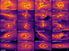 |
Fig. 1. Projection of gas density, within the 10 Reff thick slices, of representative galaxies at different redshifts (rows) and stellar masses (columns). Dashed circles show the effective radius of the stellar component (see Sect. 2.2 for the definition), and the white horizontal bars indicate a 1 kpc scale. |
Number of galaxies and median of their stellar mass (in log M⊙) used in our analysis, at each redshift.
2.3. Fitting method
To quantify the correlation between the surface densities of gas and the SFR, we fit the distributions with the relation logΣSFR = a(logΣgas)+b, with the best-fit values for the slope a and intercept b. In this paper, we do not attempt to provide a thorough study of the impact of different fitting methods used in the literature on the estimated values for the obtained parameters (we refer the readers to, e.g., Hogg et al. 2010, for a discussion on fitting methods used in science). Nevertheless, we compare three different fitting methods: the ordinary least square (OLS) technique, the OLS bisector technique (Isobe et al. 1990), and the Bayesian linear regression (BLR). The results of the Bayesian regression are shown throughout the paper, as it provides a more robust treatment of errors and is thus particularly adapted to observational measures. In Appendix B, we report the results of the OLS bisector, together with a more detailed comparison of different methods. In short, all three fitting methods provide a qualitatively similar trend for the slopes and dispersions around the best fit as a function of redshift and stellar mass. We note, however, that quantitatively, the values of the slope differ: they are systematically higher for the bisector OLS method, and the dispersion around the best fit is also systematically higher. Overall, depending on the population of galaxies and the gas tracer under consideration, the choice of the fitting method can produce changes of 10% to 30% for the slope, in agreement with similar estimates of the impact of fitting algorithms on recent observational data (see de los Reyes & Kennicutt 2019; Kennicutt & De Los Reyes 2021). These differences should be kept in mind when comparing the values reported in the literature.
3. Results
3.1. Distributions of galaxies in the KS plane
We started by investigating the diversity of star-forming galaxies and its evolution with cosmic time, by analyzing the distributions of galaxies in the KS plane in different stellar mass bins and as a function of redshift. Figure 2 shows the distribution of galaxies of the NEWHORIZON simulation in the ΣH2 − ΣSFR plane, in different stellar mass bins (columns) at different redshifts (rows), color-coded by their sSFR (sSFR = SFR/M⋆), computed for the entire galaxy with the same timescale as ΣSFR.
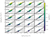 |
Fig. 2. Distribution of galaxies in the KS plane at different redshifts (rows) and in four equally populated stellar mass quartiles at each redshift (columns). The mass range of each quartile is shown in square brackets (in log M⊙). The colors indicate the sSFR of the galaxies, measured over a timescale of 10 Myr. Dash-dotted lines are fits at each redshift and mass bin, with the slopes (a) and the standard deviation of residuals of the best-fit relation (σ) shown in the lower-right corners. The coefficient R, shown at the bottom right of each panel, is the Pearson correlation coefficient. The solid black and dotted black lines show the sequence of disks and starbursts, respectively, from Daddi et al. (2010) for reference. Note, however, that our fitting method differs from theirs. Regardless of stellar mass, the distributions of galaxies move within the KS plane toward lower values of ΣH2 and ΣSFR with decreasing redshift. At each redshift and in each stellar mass bin, the sSFR of galaxies strongly correlates with ΣSFR. Figure A.1 shows the same but using the neutral gas. |
Although the distributions vary quite significantly between panels, at a given redshift, there is a substantial overlap in the range of values of both ΣH2 and ΣSFR within the KS plane. The lowest and highest tails of these distributions at each redshift are typically dominated by galaxies within the lowest and highest stellar mass bins, respectively. Overall, the distributions of galaxies of a given stellar mass quartile move within the KS parameter space toward lower values of ΣH2 and ΣSFR with decreasing redshift: fewer and fewer galaxies are found far above the canonical KS relation4 (solid line), at all stellar masses. This is accentuated after cosmic noon (z < 2) where only a handful of galaxies reach the sequence of starbursts (dotted line).
As expected, the sSFR of galaxies decreases with decreasing redshift, in particular at z ≤ 2. It also decreases with increasing stellar mass at each redshift. The sSFR of galaxies strongly correlates with ΣSFR at each redshift and in each stellar mass bin, essentially because the sSFR is computed using stars with the same age as ΣSFR (< 10 Myr). This strong correlation vanishes when considering older stars (e.g., < 100 Myr). As a consequence, at fixed ΣH2, galaxies with shorter depletion times, have a higher sSFR than those with longer depletion times. We stress that this behavior, although not surprising, is not obvious. Starbursting systems have short depletion times (i.e., the normalization of the SFR by the gas mass5), while the sSFR is the SFR normalized by the stellar mass. Galaxies with a given sSFR but different gas fractions could then have significantly different depletion times. As a matter of fact, the systematic qualification of starburst galaxies as outliers above the main sequence of star formation is being questioned by observations (Gómez-Guijarro et al. 2022; Ciesla et al. 2023; see also, e.g., Tacconi et al. 2018) and simulations (Renaud et al. 2022).
The trends and correlations from Fig. 2 persist when the neutral gas (ΣH I+H2) is considered instead of the molecular gas alone (ΣH2; see Fig. A.1), but with a steepening of the slopes, weakening of correlations, and increased scatter, in agreement with observations, at all redshifts and in all stellar mass bins.
Figure 3 shows the distributions in the ΣH2 − ΣSFR and ΣH I+H2 − ΣSFR planes, but now for the entire population of galaxies at different redshifts, by stacking all galaxies from Figs. 2 and A.1, respectively, where 2D histograms are computed by averaging the color-coded quantity in each bin. The gradients in the sSFR seen in individual stellar mass bins are still apparent when stacking all stellar masses. Similarly, the entire galaxy population shows a stronger correlation, smaller dispersion, and shallower slope between the SFR density and the molecular gas, than with the neutral gas (this is further discussed in Sect. 3.2).
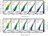 |
Fig. 3. Same as Figs. 2 and A.1, but without binning the stellar masses, and considering the molecular gas only (top) and the neutral gas (bottom). The correlation between the sSFR and ΣSFR seen in different stellar mass bins (Fig. 2) is still apparent when stacking all galaxies. At all redshifts, the slope (a) and the dispersion (σ) around the best-fit relation (dash-dotted line) are larger for the neutral gas than for the molecular gas. At all redshifts, the correlation is stronger for molecular gas than for neutral gas. |
The shallower slope of the correlation with H2 is consistent with studies of nearby galaxies both on galactic (e.g., Kennicutt 1998; Liu et al. 2015; de los Reyes & Kennicutt 2019; Kennicutt & De Los Reyes 2021) and sub-kiloparsec scales (e.g., Kennicutt et al. 2007; Bigiel et al. 2008; Leroy et al. 2008). Although the value of the slope depends on the employed fitting method and types of galaxies under consideration, it is found to be approximately linear. The relation between the SFR and the total gas surface densities for a combined sample of normal and starburst galaxies is found to be superlinear with slopes of 1.4 − 1.5 (Kennicutt 1998; Kennicutt & De Los Reyes 2021). A similar slope is found for a sample of nearby normal spiral galaxies (de los Reyes & Kennicutt 2019) and at higher redshifts (z ∼ 1.5; Daddi et al. 2010), while the inclusion of dwarf galaxies tends to produce a shallower slope of ∼1.3 (de los Reyes & Kennicutt 2019). When fitted separately, starburst galaxies appear to follow a relation with slope 1 − 1.2, as recently revealed by Kennicutt & De Los Reyes (2021), which is shallower compared to previous studies finding slopes of 1.3 − 1.4 (e.g., Kennicutt 1989; Daddi et al. 2010), but confirms bimodal (or possibly multimodal) relation for the global star formation (e.g., Daddi et al. 2010; Genzel et al. 2010).
We now explore when these observed relations emerge.
3.2. Emergence of the KS relation
The redshift dependence of the trends highlighted in the previous section suggests that the KS relation evolves with cosmic time. In this section, we explore its emergence and overall evolution. Figure 4 shows the evolution of the slope a of the relations ( ) fitted with the BLR method, and Fig. 5 displays the dispersion of the data around these fits (see Appendix B.3 for the equivalent plots using another fitting method providing qualitatively similar trends, though with notable quantitative difference).
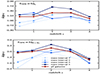 |
Fig. 4. Evolution of the slope of the fits of the KS relation from Figs. 2 and A.1, i.e., using the Bayesian fitting method, for the four mass bins considered, from the low-mass bin in a light color to the most massive one in a dark color. The red points show the slope of the entire galaxy population at a given redshift (i.e., without accounting for their mass, as in Fig. 3). After z ≈ 2 − 3, the slope of the KS relation for the two most massive bins remains within 30% (respectively 37%) of its final, converged, value for the molecular (respectively neutral) gas, which indicates the emergence of the KS relation at these redshifts. Low-mass galaxies do not show signs of convergence toward a fixed slope: their KS relation gets continuously shallower after z ≈ 2 − 3. |
The least massive galaxies (the lower half of the stellar mass distribution) clearly differ from the most massive cases (the highest stellar mass bin): at all redshifts, their KS relations are shallower and more dispersed. An examination of the distributions (Fig. 2) reveals that this originates from the presence of galaxies with short depletion times at low ΣH2. Such cases of rapid star formation in (relatively) diffuse gas possibly due to environmental triggers like mergers, or strong (or fast) gas outflows, are found at low masses at all redshifts, but only at high redshifts for the massive quartiles. At cosmic noon (z ∼ 2), this regime disappears at all masses but reappears at z ≲ 2 at low masses. This explains the overall “bell” shape at low masses in Fig. 4. This effect is significantly more pronounced in the neutral gas (H I + H2), which indicates that the fraction of molecular over neutral gas plays a role in star formation in diffuse gas. It is likely that at the lowest masses, the galaxies comprise only one active star-forming region at a given instant (i.e., a molecular cloud with an extended atomic envelope; recall Fig. 1), which would favor the star formation regime noted here.
The slope of the KS relation stabilizes below z ≈ 2 for the overall population (red thick line on Fig. 4) and the most massive galaxies (M⋆ ≳ 108 M⊙ at this redshift). This is also the epoch when the dispersion around the relation reaches its final, minimum plateau (Fig. 5). Therefore, the present-day KS relation emerges at cosmic noon (z ≈ 2) in the most massive galaxies. Our results predict that populating the KS plane with observational data from the top 50% most massive galaxies at redshifts ≳3 would result in a different and significantly more dispersed relation than the one currently established at low and intermediate redshifts (when considering local spirals, z = 1 − 2 disks, and the so-called BzK color-selected galaxies, Daddi et al. 2010; Tacconi et al. 2010; Salmi et al. 2012).
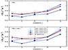 |
Fig. 5. Same as Fig. 4, but showing the dispersion around the best fit. Only the vertical dispersion, i.e., in log(ΣSFR), is considered here. |
However, this is not the case for the least massive galaxies, for which no stabilization of the slope is seen, neither in molecular nor neutral gas. Interestingly, the dispersion around the best fit of these galaxies still yields a behavior very similar, qualitatively and quantitatively, to that of the most massive ones: a decrease until z ≈ 2 − 3 followed by a relatively flat plateau. Hence, the relation for the low-mass galaxies becomes simultaneously tighter and shallower below z ≈ 2 − 3. This could indicate that the extreme cases at high redshifts either evolve to a more massive quartile via rapid growth or conversely get quenched and disappear from the star-forming sample. The remaining low-mass objects would then display a more homogeneous behavior.
These shallower KS relations of low-mass galaxies are in qualitative agreement with the observations of local dwarf galaxies, which report slopes around unity (e.g., Filho et al. 2016; Roychowdhury et al. 2017)6. The underlying reason is still debated and probably consists of an interplay between galaxy interactions and the low-metallicity contents of these dwarf galaxies, which caps their efficiency at forming molecular gas (Cormier et al. 2014). Such hypotheses are in line with our measurements of star formation in diffuse gas that we interpret as star-forming regions with extended atomic envelopes. Confirming these ideas requires a resolved analysis of these galaxies, instead of the statistical approach we follow here. Thus, we will explore these hypotheses in a forthcoming paper.
When considering the relation between ΣSFR and the neutral gas surface density ΣH I+H2, we retrieve qualitatively the same evolution of the slope and the dispersion with redshift and stellar mass (for all mass quartiles), but with steeper slopes. The reason for this steepening of the relations is the presence of sub-efficient star-forming regions in galaxies at low ΣH I+H2, often referred to as the “break” of the KS relation (see an illustration in Bigiel et al. 2008). The physical origin of the break has been shown analytically (Renaud et al. 2012) and numerically (Kraljic et al. 2014) to be caused by low levels of turbulence, which do not efficiently promote the formation of dense gas, or in other words, by a low filling factor of star-forming gas in the volumes considered. In turn, the break becomes more apparent when including the atomic component in our analysis, by increasing the gas surface density without altering ΣSFR, which bends the distribution of galaxies in the KS plane below the canonical KS relation.
At low redshifts, the low-mass galaxies of our sample correspond to dwarfs of which the low-metallicities (Dubois et al. 2021) could explain the inefficient formation of molecular gas (at small scales), and in turn slow down star formation, even at high ΣH2 at galactic scales (but see the discussion of Roychowdhury et al. 2017 on the relatively small effect of the metallicity on the KS relation). Interestingly, Fig. 13 of Dubois et al. (2021) indicates that the relation between the stellar mass and the metallicity in NEWHORIZON varies only very weakly with the redshift. We checked that this remains true when selecting the star forming galaxies only. We confirm that the gas and stellar metallicities7 for the selection of galaxies within the KS plane increase with stellar mass and with decreasing redshift, as expected, but the redshift evolution of the mass-metallicity relation is only weak. Moreover, at all redshifts, at a given stellar mass, the metallicity does not show any gradient within the KS plane. This implies that low-redshift dwarfs have a similar metallicity as the galaxies with the same stellar mass at z ≳ 2, but which are then in our upper mass bin, and already follow distributions close to the canonical KS relation. This demonstrates that the stellar mass and the metallicity are not key parameters in driving the emergence of the KS relation. The role of other physical quantities is explored in the next section.
3.3. Physical drivers of the KS relation
3.3.1. Molecular and total gas content
We now investigate whether the relation between ΣH2 and ΣSFR is driven by the gas content of galaxies.
Figure 6 (top panel) shows the molecular gas fraction, defined as the fraction of H2 mass over the neutral gas (i.e., MH2/(MH I + MH2)), and its evolution within the KS plane with the cosmic time for the entire galaxy population. The fraction of molecular gas decreases with decreasing redshift. Moreover, it correlates with ΣH2 resulting in vertical contours (within the KS plane) at all redshifts. The same trends are seen at a given stellar mass, although the fraction of molecular gas increases with stellar mass (Fig. A.2; see also Dubois et al. 2021, their Fig. 19).
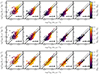 |
Fig. 6. Same as Fig. 3, but color-coded by the molecular over cold gas fraction (top), and baryonic molecular (middle) and neutral (bottom) gas fractions. The molecular gas fraction (top panel) correlates with ΣH2 at all redshifts. The baryonic molecular fraction (middle panel) correlates with ΣH2 at high redshifts; below z ∼ 2 this correlation weakens and is essentially carried by low-mass galaxies. The correlation between the neutral gas fraction and ΣH2 is apparent only at z = 4. At z ≲ 2 the trend reverses, meaning this fraction decreases with increasing ΣH2. |
The molecular gas content of galaxies can also be defined in terms of baryonic fraction: MH2/(MH I + MH2 + M⋆). The correlation between the baryonic molecular gas fraction and ΣH2 is maintained at all redshifts (Fig. 6, middle panel), although it weakens at z ≲ 2 when it is only carried by the low-mass galaxies – the massive galaxies having very low baryonic molecular gas fraction, independently of ΣH2 (see Fig. A.3). This lack of correlation at low redshifts results from the baryonic fraction of molecular gas versus stellar mass relation getting shallower at these late times (see the top-right panel of Fig. 19 of Dubois et al. 2021).
We finally considered the neutral baryonic gas fraction: (MH I + MH2)/MH I + MH2 + M⋆). As already reported by Dubois et al. (2021) for the NEWHORIZON galaxies, this fraction strongly anticorrelates with the stellar mass, but only mildly depends on the redshift at a given mass. This is confirmed in the KS plane for galaxy stacks (Fig. 6, bottom panel) and individual stellar mass bins (Fig. A.4). At high redshifts (z = 4), the neutral gas fraction increases with ΣH2 for all stellar masses, but this correlation disappears at later epochs, where this fraction varies weakly with ΣH2 at fixed stellar mass but varies strongly with stellar mass. The combination of these relations between the neutral gas fraction and ΣH2 at high z, and M⋆ at all z, translates into a nontrivial evolution of the distributions of the neutral gas fraction in the KS plane when the stellar mass is marginalized out. The reversal of the trend between the neutral gas fraction and ΣH2 between high and low redshifts is thus a direct consequence of the dependences highlighted above, and of how early the galaxies build up their stellar masses.
In conclusion, both the molecular and neutral gas fractions vary with one of the parameters of the KS plane (ΣH2), but have close to no influence on the other (ΣSFR), except in the very diffuse gas of the low-mass galaxies, as noted above. As such, at galactic scales, the KS relation does not originate from the gas fractions of the galaxies, at any redshift, nor at any stellar mass. The quantity that correlates better within the KS plane is the fraction of cold gas that is in the dense phase; however, it does not fully capture the variation with both the surface density of gas and the SFR of galaxies.
3.3.2. Turbulence
Previous works (e.g., Vazquez-Semadeni 1994; Renaud et al. 2014) have pointed out the role of turbulence in setting the density distributions of gas, and thus the amount of star-forming gas in galaxies. We tested whether turbulence explains the emergence of the KS relation over cosmic time.
Figure 7 shows the distribution of galaxies in the KS plane, now color-coded with their turbulence Mach number ℳ. At all redshifts, ℳ evolves monotonically along the best-fit relation in the KS parameter space, by increasing with ΣH2 and ΣSFR. Furthermore, at fixed ΣH2, ΣSFR is positively correlated with ℳ.
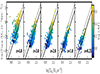 |
Fig. 7. Same as Fig. 3, but color-coded by the Mach number, ℳ. At all redshifts, ℳ increases monotonically with both increasing ΣH2 and ΣSFR. At fixed ΣH2, ℳ is correlated with ΣSFR. |
As shown in Fig. A.5, these trends are independent of the galaxy’s stellar mass. At fixed stellar mass, galaxies at high redshifts are more turbulent than their low-redshift counterparts, and at fixed redshift, more massive galaxies tend to be more turbulent than their lower-mass counterparts, a direct consequence of increasing gas richness in galaxies with redshift (e.g., Bournaud et al. 2010; Renaud et al. 2012).
To investigate the physical origin of these trends, Fig. 8 shows the distributions of the Mach number,  , and the underlying quantities, which are the gas velocity dispersion (σvel) and the temperature (T)8. While the velocity dispersion decreases with redshift for all mass bins, only massive galaxies maintain high values at low z (∼10 km s−1), leading to significantly higher median values. This is confirmed by observations at low redshifts of lower dispersion in dwarf galaxies (∼1 km s−1) than in massive galaxies (∼10 km s−1; e.g., Hunter et al. 2021). This general trend likely originates in parts from the overall lowering of the star formation activity with cosmic time, and possibly the less efficient coupling of feedback with the local ISM, as opposed to intergalactic medium due to low escape velocity, in low-mass galaxies (i.e., with shallow potential wells).
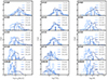 |
Fig. 8. Normalized distributions of gas velocity dispersion (left), temperature (middle), and Mach number (right) in different stellar mass bins (colored lines, as indicated in the legend, report the logarithm of M⋆ in units of M⊙) and redshifts (indicated in the upper-left part of each panel). Vertical lines represent medians of distributions. |
The locations of the galaxies with high σvel in the KS plane (Fig. A.6) reveal complex correlations with the indicators of star formation: while galaxies with short depletion times tend to have high σvel, high-velocity dispersion are found across the entire KS plane. This indicates that stellar feedback is not the only factor in setting the velocity dispersion, and therefore the KS relation (see also Agertz et al. 2011; Agertz & Kravtsov 2015), at the galactic scale. Galactic dynamics and interaction-triggered stirring are likely important drivers of the velocity dispersion (see Renaud et al. 2014 for an illustration that increased velocity dispersion is a cause and not a consequence of starbursts in mergers).
The temperature of all mass quartiles decreases with decreasing redshift, but Fig. 8 (middle-column) reveals that the stellar mass only discriminates the distributions of T at late times (z ≲ 1). Contrary to the velocity dispersion, there is no relation between the star formation indicators and the temperature in the KS plane (Fig. A.7), which is consistent with the interpretation of the limited impact of feedback, even though the details, in particular on small scales, might be more complicated.
In terms of Mach number, the trends noted from the two underlying quantities (σvel and T) naturally combine to lead to a shift in the distributions of ℳ toward low values with decreasing redshift. This effect is significantly more pronounced for low-mass galaxies (Fig. 8).
A more detailed examination (Fig. A.5) reveals that the trends found in the velocity dispersion and temperature conspire to give rise to a clear evolution of ℳ along the KS relation, with a “tighter correlation” with Σgas and ΣSFR than the individual σvel and T. This further demonstrates the paramount role of turbulence in the star formation activity, in particular in the KS plane.
Higher Mach numbers favor higher density contrasts in the ISM (i.e., a wider gas density probability density function; see Federrath et al. 2008), and thus the formation of a larger faction of dense molecular gas. This explains that dwarf galaxies at low redshifts, with a low Mach number, tend to have lower molecular gas fractions (Fig. A.2) than their massive counterparts, and thus appear below the canonical KS relation, in the so-called “break” (see Kraljic et al. 2014), when considering the total neutral gas (Fig. A.1), but are shifted toward the low gas densities when considering the molecular phase only (Fig. 2). Finally, the high ΣSFR of these galaxies implies that this shift toward low ΣH2 places them above the canonical KS relation, which drives the flattening of the relation of these subpopulations (recall Fig. 4).
Furthermore, the histograms of Fig. 8 show that the distributions of velocity dispersion in low-mass galaxies become peaked toward the low-value end at low redshifts, while the massive galaxies only exhibit a tail with only a few cases at such low-velocity dispersion, and the bulk of their distribution remains centered around higher values (∼10 km s−1) with little evolution after z ≲ 2. In other words, the lower end of the distributions in σvel gets more and more populated with low-mass galaxies with decreasing redshift, while the distribution of velocities dispersion of massive galaxies ceases to evolve (statistically). For the reasons discussed before, this transpires in the histograms of Mach number, and finally in the distribution of galaxies in the KS plane. Therefore, the mass-dependent evolution of the velocity dispersion explains the convergence of the slope of the KS relation at high masses after z ≈ 2, and the absence of the convergence in low-mass galaxies, noted in Fig. 4.
4. Discussion
4.1. Scale and projection effects
So far, we have conducted our analysis using the observables ΣH2, or ΣH I+H2, and ΣSFR, and identified relations in the KS plane. However, by doing so, we effectively introduce an arbitrary choice for the spatial scale used in the measurement of both quantities, which necessarily impacts the values of the surface densities and possibly artificially distorts the distributions of galaxies in the KS plane. To establish whether our conclusions depend on our choice of examining projected quantities, and over the scale of the effective radius, we plot in Fig. 9 the distributions of galaxies of our sample in the plane of molecular gas mass versus SFR, that is to say, a deprojected version of the KS plot, color-coded by mass (top) and size Reff (bottom). At all redshifts, more massive galaxies tend to have higher SFRs and higher molecular gas masses; however, there is no obvious correlation between the SFR, MH2, and the effective radius of galaxies. Furthermore, all the trends (or the absence thereof) with molecular and total gas fractions, and ℳ seen in the KS parameter space are retrieved with deprojected quantities, as shown in Fig. C.1. Therefore, the trends seen in the KS plane are not primarily driven by measuring the physical quantities in projection rather than in 3D, and the scale adopted does not introduce biases in the distributions.
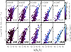 |
Fig. 9. Distribution of galaxies in the MH2–SFR plane, i.e., a deprojected version of the KS plane, at redshifts 4, 3, 2, 1, and 0.25, from left to right, as a function of galaxy mass (top) and effective radius (bottom). Dash-dotted lines are fits in the logarithmic space at each redshift, with the slope, a, and the standard deviation of residuals, σ. The coefficient R is the Pearson correlation coefficient. At all redshifts, more massive galaxies tend to have higher SFRs and MH2 values compared to their lower-mass counterparts. As galaxies grow in mass, they also grow in size; however, no obvious correlation is seen between Reff, the SFR, and the molecular gas mass. |
The diversity of star formation activities seen in the wide distribution of ΣH2, ΣH I+H2, and ΣSFR, but also in the slopes and the scatters of the KS relation, results from the convolution of two other effects: (i) the diversity of galaxies in the sample, illustrated by the variations of the KS relations with stellar mass and redshift (Fig. 2), and (ii) the integration of the local, small-scale star formation law over entire galactic scales where not all the ISM is star-forming. Indeed, the shape (slope, offset, break, and scatter) of the distributions of galaxies in the KS plane is driven by the underlying distribution of the physical properties of the star-forming regions within each galaxy, and it is the evolution of these distributions as functions of redshift, galactic mass, and other factors, such as the environment, that sets the evolution of the KS relations.
4.2. Sub-grid models
Our work highlights the key role of turbulence (Mach number) in driving the KS relation at the galactic scale, including at high redshifts. This confirms the analytical results of Renaud et al. (2012) and the numerical work of Kraljic et al. (2014), who conducted a similar study without cosmological context and for galaxies in the nearby Universe only (i.e., at low gas fractions). We note that the star formation model in Kraljic et al. (2014) differs from those in NEWHORIZON, as it uses a fixed star formation efficiency per free-fall time and is applied at a higher resolution (∼1 pc). In other words, the right-hand side of Eq. (1) used in the latter reduces to a constant value in the former. The paramount role of turbulence in setting the KS relation found with both models (independently of an explicit inclusion of turbulence in the star formation model in the latter), further strengthens our conclusion.
Yet, it is important to keep in mind that the differences in the sub-grid models used do not necessarily correspond to different physics. Schemes that do not capture the formation of star-forming clouds (i.e., at resolutions ≳20 pc) ought to incorporate this aspect in their star formation prescription. This can be achieved by imposing a criterion on the instability of the gas, through, for example converging flows and/or the virial parameter, as is done in NEWHORIZON. However, at cloud scales (≈1 − 10 pc), the fragmentation of the ISM into individual clouds is already captured by the simulations, and so an instability criterion is redundant: at high resolution, the dense gas has necessarily gone through the instability phase. As for any physical mechanism, it is crucial to identify which processes are not captured explicitly by the simulation, in order to construct and parametrize the “sub” aspect of the sub-grid models.
By conducting a spatially resolved study of the KS relation within the FIRE (Hopkins et al. 2014) framework, Orr et al. (2018) pinpointed instead the central role of stellar feedback in regulating star formation at small scales (see also Dekel et al. 2019, for similar conclusion for the global KS relation). We note, however, that their sub-grid treatment de facto implies an important role for feedback, as it is required to regulate the star formation process set with an efficiency of 100% (as opposed to ∼0.1 − 10% in most of the literature from observations and simulations). Grisdale et al. (2019) showed that even imposing a fixed star formation efficiency per free-fall time in the sub-grid recipe leads to a wide diversity of effective efficiencies across the population of star-forming clouds, with or without feedback. However, feedback impacts not only the local regulation of star formation but leaves also an imprint on other aspects like the turbulence spectrum and the structure of the ISM at kiloparsec scales. Therefore, even if widely different sub-grid recipes can be parametrized to produce similar star formation activities, they likely leave diverging signatures on other aspects and at different scales. It is, therefore, possible that by adopting a lower star formation efficiency and thus automatically decreasing the impact and role of feedback in the inefficiency of star formation, the FIRE framework could still reproduce observables, like the KS relations, and yet lead to different conclusions on its physical driver, perhaps more similar to our results (see, e.g., Brucy et al. 2020, 2023; Hu et al. 2023). For instance, in the analytical model of Renaud et al. (2012), stellar feedback can be introduced as a cap on the effective star formation efficiency. While this results in lowering the slope of the KS relation, a requirement to match observations, a KS-like power-law does exist without feedback, and originates solely from the log-normal shape of the distribution of gas density, itself known to be set by turbulence (e.g., Vazquez-Semadeni 1994). The fact that the KS relation can be modeled from such different underlying physics suggests that divergences should be sought in more fundamental quantities or behavior, and possibly at smaller scales, that is to say, before the differences between models get blended in integrated, projected, and galactic-scale averaged measurements. Considering other, more extreme environments where the relative contributions of the mechanisms involved vary could certainly provide interesting insights.
4.3. A variety of possible underlying physical mechanisms
Taking advantage of the broad diversity of galaxies in NEWHORIZON, we show here that the gas fraction does not strongly influence the star formation relation, at least when integrated over entire galaxies, and that the mild trends found between the gas fraction and its surface density (be it neutral or molecular) actually get reversed at z ≈ 2. This change entails an evolution of the morphology and size of the star-forming volume, likely connected to a more concentrated activity. Underlying physical reasons could be: the intrinsic evolution of disks toward fueling more and more gas to the nuclei and/or environmental effects due to gravitational torques exerted on disk material by more and more massive companion galaxies.
Some of these aspects have been explored in the special case of the Milky Way-like galaxy, using the VINTERGATAN simulation (Agertz et al. 2021; Renaud et al. 2021a). These works highlight the necessity for the galactic disk to be in place (Park et al. 2021) for the galaxy to strongly react via large-scale wakes to interactions through a starburst activity (Segovia Otero et al. 2022). The redshift-dependence of tidal compression, both in terms of intensity and mass involved also appears as crucial in the cosmic evolution of starbursts (Renaud et al. 2022) as it controls energy input at the cascade injection scale. Exploring these points further and over an entire population of galaxies, like that in NEWHORIZON, requires a dedicated analysis of the diversity of individual evolution that builds the population statistics shown here, which we leave for a forthcoming paper (Kraljic et al., in prep.).
Galaxies with the highest global turbulence level are not only those that host the densest gas and form the most stars (as shown by their locations at high surface densities of gas and of SFRs). They are also the galaxies with the shortest depletion time. This is particularly visible at high redshifts (z ≳ 2) in Fig. 7, where the most turbulent galaxies lie around the starburst relation from Daddi et al. (2010), about 1 dex above the canonical KS relation. This is in line with the conclusions of Renaud et al. (2014, 2019b, 2021b), who reported that the increase in the level of compressive turbulence in mergers can lead to a starburst activity. In this context, it is crucial to differentiate the production of many stars (high SFRs) from the fast production of stars (short depletion time). While the two aspects are independent, our results show that high levels of turbulence make some high-redshift galaxies reach both a high ΣSFR, and a short depletion time. This then changes at lower redshifts, when the most turbulent galaxies of our sample do not necessarily yield the shortest depletion times. Such an evolution could be connected with the rarefaction of the major mergers at late epochs, and thus the statistical lowering of the tidal and turbulent compression (Renaud et al. 2022), and likely has implications on the evolution of the normalization of the main sequence of galaxy formation (e.g., Tacconi et al. 2018).
5. Conclusion
We have investigated the distributions of galaxies from the cosmological hydrodynamic simulation NEWHORIZON in the KS parameter space, as a function of their stellar masses and redshifts, the emergence and physical drivers of the star formation scaling laws at galactic scales. Our main results are:
-
Both the stellar mass and redshift influence the overall location of the galaxy population in the KS plane.
-
A power-law relation of the form
 with a slope a ≈ 1.4 emerges at z ≈ 2 − 3 for the more massive half of the galaxy population (M⋆ ≳ 108 M⊙ at these redshifts), in agreement with observations up to these redshifts. However, the slope of the relation varies at earlier epochs, with an increased scatter. This indicates that the KS relation might not provide a robust calibration for star formation in galaxies at very high redshifts. For the least massive galaxies, there is no sign of a convergence of the slopes of their distribution in the KS plane, because it continues to get shallower at the last epochs. The slopes are systematically higher when considering the total neutral gas as opposed to the molecular gas. At all stellar masses, the dispersion around the best-fit relation decreases with decreasing redshift.
 -
The gas fraction (neutral or molecular) does not correlate with the star formation activity as traced by ΣSFR and therefore does not play a primary role in establishing the KS relation. Similarly, neither the velocity dispersion of the gas nor its temperature can fully explain the star formation activity of galaxies as captured by the KS relation, pointing toward a limited impact of feedback.
-
Conversely, the level of turbulence of the ISM, as quantified by the Mach number, is found to drive the relation between gas and SFR densities at all redshifts, independent of stellar mass. More specifically, it is the ability of a galaxy to reach a supersonically turbulent regime that matters, with the Mach number (ℳ > 1) being the driver of the KS relation, independent of stellar mass. At high redshifts, for a given gas density, the most turbulent galaxies yield short depletion times, which are characteristic of starburst galaxies. Their frequency decreases at low redshifts.
The evolution reported here and in a number of previous works on the star formation activity at galactic scales points toward an important role of inflow, interactions, mergers, and the proximity of the disk to marginal stability in driving the star formation relations and their scatters. The proximity of the disk to marginal stability could act as a confounding factor for an efficient turbulent cascade and star formation, explaining the emergence of tighter KS scaling relations, when secular dissipative processes take over. Exploring these aspects requires tracking individual galaxies along their merger histories and looking for changes in the properties of the star-forming material during the starburst phases, both at cloud and galactic scales. We will cover these topics in the forthcoming papers of this series.
http://new.horizon-simulation.org
Given that NEWHORIZON is a zoom simulation embedded in a larger cosmological volume filled with lower dark matter resolution particles, some halos of the zoom regions can be polluted with low-resolution dark matter particles.
However, considering the molecular gas alone yields qualitatively similar results (not shown).
With the term canonical, we refer to the sequence of normal, star-forming disks, as defined in, e.g., Daddi et al. (2010), i.e.,  .
.
As such, lines of constant depletion time have a slope of unity in the KS plane. A slight difference exists with the observed sequence of starbursts, which yields a slope of 1.4 in the KS plane (Daddi et al. 2010). This nuance is yet to be understood.
As mentioned in the previous section, a quantitative agreement cannot be reached due to the diversity of fitting methods employed in the literature.
The metallicity is computed within the Reff. For the gas metallicity, only the neutral phase is considered.
As in the case of velocity dispersion and the Mach number, the temperature is also computed as a mass-weighted average of gas cells within the Reff. Therefore, the temperature values are not directly comparable to typical values within individual molecular clouds.
We used the probabilistic programming package for Python PYMC3, available at https://docs.pymc.io/en/v3/index.html.
We used the Python package implementing the linmix algorithm available on github at https://github.com/jmeyers314/linmix.
Acknowledgments
The authors thank the anonymous referee for insightful comments. This work was granted access to the high-performance computing resources of CINES under the allocations c2016047637 and A0020407637 from GENCI, and KISTI (KSC-2017-G2-0003). Large data transfer was supported by KREONET, which is managed and operated by KISTI. This work relied on the HPC resources of the Horizon Cluster hosted by Institut d’Astrophysique de Paris. We warmly thank S. Rouberol for running the cluster on which the simulation was post-processed. F.R., O.A., E.A., and A.S.O. acknowledge support from the Knut and Alice Wallenberg Foundation and the Swedish Research Council (grant 2019-04659). F.R. acknowledges the support provided by the University of Strasbourg Institute for Advanced Study (USIAS), within the French national programme Investment for the Future (Excellence Initiative) IdEx-Unistra. E.A. acknowledges support from US NSF grant AST18-1546. S.K. acknowledges support from the STFC [grant numbers ST/S00615X/1 and ST/X001318/1] and a Senior Research Fellowship from Worcester College Oxford. T.K. was supported by the National Research Foundation of Korea (NRF) grant funded by the Korean government (No. 2020R1C1C1007079). S.K.Y. acknowledges support from the Korean National Research Foundation (2020R1A2C3003769). This work was supported in part by the Korean National Research Foundation (2022R1A6A1A03053472). This work is partially supported by the grant Segal ANR-19-CE31-0017 of the French Agence Nationale de la Recherche and by the National Science Foundation under Grant No. NSF PHY-1748958.
References
- Agertz, O., & Kravtsov, A. V. 2015, ApJ, 804, 18 [NASA ADS] [CrossRef] [Google Scholar]
- Agertz, O., Teyssier, R., & Moore, B. 2011, MNRAS, 410, 1391 [Google Scholar]
- Agertz, O., Renaud, F., Feltzing, S., et al. 2021, MNRAS, 503, 5826 [NASA ADS] [CrossRef] [Google Scholar]
- Alves, J., Lombardi, M., & Lada, C. J. 2007, A&A, 462, L17 [NASA ADS] [CrossRef] [EDP Sciences] [Google Scholar]
- Andersson, E. P., Renaud, F., & Agertz, O. 2021, MNRAS, 502, L29 [NASA ADS] [CrossRef] [Google Scholar]
- André, P., Men’shchikov, A., Bontemps, S., et al. 2010, A&A, 518, L102 [NASA ADS] [CrossRef] [EDP Sciences] [Google Scholar]
- Appleby, S., Davé, R., Kraljic, K., Anglés-Alcázar, D., & Narayanan, D. 2020, MNRAS, 494, 6053 [NASA ADS] [CrossRef] [Google Scholar]
- Aubert, D., Pichon, C., & Colombi, S. 2004, MNRAS, 352, 376 [Google Scholar]
- Bigiel, F., Leroy, A., Walter, F., et al. 2008, AJ, 136, 2846 [NASA ADS] [CrossRef] [Google Scholar]
- Bigiel, F., Leroy, A. K., Walter, F., et al. 2011, ApJ, 730, L13 [NASA ADS] [CrossRef] [Google Scholar]
- Bolatto, A. D., Wolfire, M., & Leroy, A. K. 2013, ARA&A, 51, 207 [CrossRef] [Google Scholar]
- Bouché, N., Cresci, G., Davies, R., et al. 2007, ApJ, 671, 303 [Google Scholar]
- Bournaud, F., Elmegreen, B. G., Teyssier, R., Block, D. L., & Puerari, I. 2010, MNRAS, 409, 1088 [CrossRef] [Google Scholar]
- Brucy, N., Hennebelle, P., Bournaud, F., & Colling, C. 2020, ApJ, 896, L34 [NASA ADS] [CrossRef] [Google Scholar]
- Brucy, N., Hennebelle, P., Colman, T., & Iteanu, S. 2023, A&A, 675, A144 [NASA ADS] [CrossRef] [EDP Sciences] [Google Scholar]
- Ciesla, L., Gómez-Guijarro, C., Buat, V., et al. 2023, A&A, 672, A191 [NASA ADS] [CrossRef] [EDP Sciences] [Google Scholar]
- Cormier, D., Madden, S. C., Lebouteiller, V., et al. 2014, A&A, 564, A121 [NASA ADS] [CrossRef] [EDP Sciences] [Google Scholar]
- Daddi, E., Elbaz, D., Walter, F., et al. 2010, ApJ, 714, L118 [NASA ADS] [CrossRef] [Google Scholar]
- de los Reyes, M. A. C., & Kennicutt, R. C., Jr. 2019, ApJ, 872, 16 [NASA ADS] [CrossRef] [Google Scholar]
- Dekel, A., Sarkar, K. C., Jiang, F., et al. 2019, MNRAS, 488, 4753 [CrossRef] [Google Scholar]
- Dubois, Y., Devriendt, J., Slyz, A., & Teyssier, R. 2010, MNRAS, 409, 985 [Google Scholar]
- Dubois, Y., Devriendt, J., Slyz, A., & Teyssier, R. 2012, MNRAS, 420, 2662 [Google Scholar]
- Dubois, Y., Pichon, C., Welker, C., et al. 2014, MNRAS, 444, 1453 [Google Scholar]
- Dubois, Y., Beckmann, R., Bournaud, F., et al. 2021, A&A, 651, A109 [NASA ADS] [CrossRef] [EDP Sciences] [Google Scholar]
- Federrath, C., & Klessen, R. S. 2012, ApJ, 761, 156 [Google Scholar]
- Federrath, C., Klessen, R. S., & Schmidt, W. 2008, ApJ, 688, L79 [NASA ADS] [CrossRef] [Google Scholar]
- Feldmann, R., Gnedin, N. Y., & Kravtsov, A. V. 2012, ApJ, 758, 127 [NASA ADS] [CrossRef] [Google Scholar]
- Filho, M. E., Sánchez Almeida, J., Amorín, R., et al. 2016, ApJ, 820, 109 [NASA ADS] [CrossRef] [Google Scholar]
- Freundlich, J., Combes, F., Tacconi, L. J., et al. 2013, A&A, 553, A130 [NASA ADS] [CrossRef] [EDP Sciences] [Google Scholar]
- Freundlich, J., Combes, F., Tacconi, L. J., et al. 2019, A&A, 622, A105 [NASA ADS] [CrossRef] [EDP Sciences] [Google Scholar]
- Genzel, R., Tacconi, L. J., Gracia-Carpio, J., et al. 2010, MNRAS, 407, 2091 [NASA ADS] [CrossRef] [Google Scholar]
- Genzel, R., Tacconi, L. J., Kurk, J., et al. 2013, ApJ, 773, 68 [NASA ADS] [CrossRef] [Google Scholar]
- Gómez-Guijarro, C., Elbaz, D., Xiao, M., et al. 2022, A&A, 659, A196 [NASA ADS] [CrossRef] [EDP Sciences] [Google Scholar]
- Grisdale, K., Agertz, O., Renaud, F., et al. 2019, MNRAS, 486, 5482 [NASA ADS] [CrossRef] [Google Scholar]
- Grisdale, K., Hogan, L., Rigopoulou, D., et al. 2022, MNRAS, 513, 3906 [NASA ADS] [CrossRef] [Google Scholar]
- Haardt, F., & Madau, P. 1996, ApJ, 461, 20 [Google Scholar]
- Hennebelle, P., & Chabrier, G. 2011, ApJ, 743, L29 [Google Scholar]
- Hogg, D. W., Bovy, J., & Lang, D. 2010, ArXiv e-prints [arXiv:1008.4686] [Google Scholar]
- Hopkins, P. F., Kereš, D., Oñorbe, J., et al. 2014, MNRAS, 445, 581 [NASA ADS] [CrossRef] [Google Scholar]
- Hu, C.-Y., Smith, M. C., Teyssier, R., et al. 2023, ApJ, 950, 132 [NASA ADS] [CrossRef] [Google Scholar]
- Hunter, D. A., Elmegreen, B. G., Archer, H., Simpson, C. E., & Cigan, P. 2021, AJ, 161, 175 [NASA ADS] [CrossRef] [Google Scholar]
- Isobe, T., Feigelson, E. D., Akritas, M. G., & Babu, G. J. 1990, ApJ, 364, 104 [Google Scholar]
- Jackson, R. A., Martin, G., Kaviraj, S., et al. 2021a, MNRAS, 502, 4262 [NASA ADS] [CrossRef] [Google Scholar]
- Jackson, R. A., Kaviraj, S., Martin, G., et al. 2021b, MNRAS, 502, 1785 [CrossRef] [Google Scholar]
- Kaviraj, S., Laigle, C., Kimm, T., et al. 2017, MNRAS, 467, 4739 [NASA ADS] [Google Scholar]
- Kelly, B. C. 2007, ApJ, 665, 1489 [Google Scholar]
- Kennicutt, R. C., Jr. 1989, ApJ, 344, 685 [Google Scholar]
- Kennicutt, R. C., Jr. 1998, ApJ, 498, 541 [Google Scholar]
- Kennicutt, R. C., Jr., & De Los Reyes, M. A. C. 2021, ApJ, 908, 61 [NASA ADS] [CrossRef] [Google Scholar]
- Kennicutt, R. C., & Evans, N. J. 2012, ARA&A, 50, 531 [NASA ADS] [CrossRef] [Google Scholar]
- Kennicutt, R. C., Jr., Calzetti, D., Walter, F., et al. 2007, ApJ, 671, 333 [Google Scholar]
- Kimm, T., & Cen, R. 2014, ApJ, 788, 121 [NASA ADS] [CrossRef] [Google Scholar]
- Kimm, T., Cen, R., Devriendt, J., Dubois, Y., & Slyz, A. 2015, MNRAS, 451, 2900 [CrossRef] [Google Scholar]
- Kimm, T., Katz, H., Haehnelt, M., et al. 2017, MNRAS, 466, 4826 [NASA ADS] [Google Scholar]
- Komatsu, E., Smith, K. M., Dunkley, J., et al. 2011, ApJS, 192, 18 [Google Scholar]
- Kraljic, K., Renaud, F., Bournaud, F., et al. 2014, ApJ, 784, 112 [NASA ADS] [CrossRef] [Google Scholar]
- Kravtsov, A. V. 2003, ApJ, 590, L1 [NASA ADS] [CrossRef] [Google Scholar]
- Krumholz, M. R., & McKee, C. F. 2005, ApJ, 630, 250 [Google Scholar]
- Leroy, A. K., Walter, F., Brinks, E., et al. 2008, AJ, 136, 2782 [Google Scholar]
- Leroy, A. K., Walter, F., Sandstrom, K., et al. 2013, AJ, 146, 19 [Google Scholar]
- Liu, L., Gao, Y., & Greve, T. R. 2015, ApJ, 805, 31 [Google Scholar]
- Martin, G., Jackson, R. A., Kaviraj, S., et al. 2021, MNRAS, 500, 4937 [Google Scholar]
- Matzner, C. D., & McKee, C. F. 2000, ApJ, 545, 364 [NASA ADS] [CrossRef] [Google Scholar]
- Narayanan, D., Krumholz, M., Ostriker, E. C., & Hernquist, L. 2011, MNRAS, 418, 664 [NASA ADS] [CrossRef] [Google Scholar]
- Onodera, S., Kuno, N., Tosaki, T., et al. 2010, ApJ, 722, L127 [NASA ADS] [CrossRef] [Google Scholar]
- Orr, M. E., Hayward, C. C., Hopkins, P. F., et al. 2018, MNRAS, 478, 3653 [NASA ADS] [CrossRef] [Google Scholar]
- Padoan, P., & Nordlund, Å. 2011, ApJ, 730, 40 [Google Scholar]
- Park, M. J., Yi, S. K., Peirani, S., et al. 2021, ApJS, 254, 2 [Google Scholar]
- Rawle, T. D., Egami, E., Bussmann, R. S., et al. 2014, ApJ, 783, 59 [NASA ADS] [CrossRef] [Google Scholar]
- Renaud, F., Kraljic, K., & Bournaud, F. 2012, ApJ, 760, L16 [NASA ADS] [CrossRef] [Google Scholar]
- Renaud, F., Bournaud, F., Kraljic, K., & Duc, P. A. 2014, MNRAS, 442, L33 [NASA ADS] [CrossRef] [Google Scholar]
- Renaud, F., Bournaud, F., Daddi, E., & Weiß, A. 2019a, A&A, 621, A104 [NASA ADS] [CrossRef] [EDP Sciences] [Google Scholar]
- Renaud, F., Bournaud, F., Agertz, O., et al. 2019b, A&A, 625, A65 [NASA ADS] [CrossRef] [EDP Sciences] [Google Scholar]
- Renaud, F., Agertz, O., Read, J. I., et al. 2021a, MNRAS, 503, 5846 [NASA ADS] [CrossRef] [Google Scholar]
- Renaud, F., Agertz, O., Andersson, E. P., et al. 2021b, MNRAS, 503, 5868 [NASA ADS] [CrossRef] [Google Scholar]
- Renaud, F., Segovia Otero, Á., & Agertz, O. 2022, MNRAS, 516, 4922 [NASA ADS] [CrossRef] [Google Scholar]
- Rosdahl, J., & Blaizot, J. 2012, MNRAS, 423, 344 [Google Scholar]
- Rosen, A., & Bregman, J. N. 1995, ApJ, 440, 634 [NASA ADS] [CrossRef] [Google Scholar]
- Roychowdhury, S., Chengalur, J. N., & Shi, Y. 2017, A&A, 608, A24 [NASA ADS] [CrossRef] [EDP Sciences] [Google Scholar]
- Salmi, F., Daddi, E., Elbaz, D., et al. 2012, ApJ, 754, L14 [NASA ADS] [CrossRef] [Google Scholar]
- Schmidt, M. 1959, ApJ, 129, 243 [NASA ADS] [CrossRef] [Google Scholar]
- Schruba, A., Leroy, A. K., Walter, F., et al. 2011, AJ, 142, 37 [NASA ADS] [CrossRef] [Google Scholar]
- Segovia Otero, Á., Renaud, F., & Agertz, O. 2022, MNRAS, 516, 2272 [NASA ADS] [CrossRef] [Google Scholar]
- Semenov, V. A., Kravtsov, A. V., & Gnedin, N. Y. 2019, ApJ, 870, 79 [NASA ADS] [CrossRef] [Google Scholar]
- Sharon, C. E., Baker, A. J., Harris, A. I., & Thomson, A. P. 2013, ApJ, 765, 6 [NASA ADS] [CrossRef] [Google Scholar]
- Shetty, R., Kelly, B. C., & Bigiel, F. 2013, MNRAS, 430, 288 [NASA ADS] [CrossRef] [Google Scholar]
- Sun, J., Leroy, A. K., Ostriker, E. C., et al. 2023, ApJ, 945, L19 [NASA ADS] [CrossRef] [Google Scholar]
- Sutherland, R. S., & Dopita, M. A. 1993, ApJS, 88, 253 [Google Scholar]
- Tacconi, L. J., Genzel, R., Neri, R., et al. 2010, Nature, 463, 781 [Google Scholar]
- Tacconi, L. J., Neri, R., Genzel, R., et al. 2013, ApJ, 768, 74 [NASA ADS] [CrossRef] [Google Scholar]
- Tacconi, L. J., Genzel, R., Saintonge, A., et al. 2018, ApJ, 853, 179 [Google Scholar]
- Teng, Y.-H., Sandstrom, K. M., Sun, J., et al. 2023, ApJ, 950, 119 [NASA ADS] [CrossRef] [Google Scholar]
- Teyssier, R. 2002, A&A, 385, 337 [CrossRef] [EDP Sciences] [Google Scholar]
- Teyssier, R., Moore, B., Martizzi, D., Dubois, Y., & Mayer, L. 2011, MNRAS, 414, 195 [NASA ADS] [CrossRef] [Google Scholar]
- Thornton, K., Gaudlitz, M., Janka, H. T., & Steinmetz, M. 1998, ApJ, 500, 95 [CrossRef] [Google Scholar]
- Trebitsch, M., Blaizot, J., Rosdahl, J., Devriendt, J., & Slyz, A. 2017, MNRAS, 470, 224 [Google Scholar]
- Trebitsch, M., Dubois, Y., Volonteri, M., et al. 2021, A&A, 653, A154 [NASA ADS] [CrossRef] [EDP Sciences] [Google Scholar]
- Vazquez-Semadeni, E. 1994, ApJ, 423, 681 [Google Scholar]
- Volonteri, M., Pfister, H., Beckmann, R. S., et al. 2020, MNRAS, 498, 2219 [Google Scholar]
Appendix A: Galaxy distribution in the KS plane
A.1. Dependence on the total gas
Figure A.1 shows the distribution of galaxies in the ΣH I+H2-ΣSFR parameter space at different redshifts (rows) and in four equally populated stellar mass quartiles at each redshift (columns). Trends with the sSFR (given by the color coding) seen when considering the molecular gas (see Fig. 2) persist. At each redshift and each stellar mass bin, the sSFR of galaxies strongly correlated with ΣSFR, and regardless of the stellar mass, the distributions of galaxies move within the KS parameter space toward lower values of ΣH I+H2 and ΣSFR with decreasing redshift.
A.2. Molecular and total gas fractions
Figure A.2 shows the molecular gas fraction, defined as the fraction of H2 mass over the neutral gas (i.e., MH2/(MH I + MH2)), and its evolution within the KS plane with the cosmic time for different stellar mass bins. As already seen for the entire galaxy population (see Fig. 6, top panel), the fraction of molecular gas decreases with decreasing redshift and it is correlated with ΣH2 at all redshifts. Figure A.2 shows that this stays true also at a given stellar mass bin, even though the molecular gas fraction typically increases with stellar mass at all considered epochs.
Figure A.3 shows the molecular gas content of galaxies defined in terms of baryonic fraction (i.e., MH2)/MH I + MH2 + M⋆)) as a function of cosmic time and stellar mass. The baryonic molecular gas fraction correlates with ΣH2 at z > 2 regardless of the stellar mass of galaxies. Below z ∼ 2, this correlation weakens and is seen only for low-mass galaxies (two lowest mass bins), while massive galaxies show a very low fraction of baryonic molecular gas.
Figure A.4 shows the neutral baryonic gas fraction (i.e., (MH I + MH2)/MH I + MH2 + M⋆)) at different redshifts and in different stellar mass bins. The neutral baryonic gas fraction is strongly anticorrelated with the stellar mass at all redshifts and evolves only weakly with redshift.
These results support the conclusions of Section 3.3.1 in that at galactic scales, the KS relation is not primarily driven by the fraction of gas in galaxies at any redshift, nor at any stellar mass.
A.3. Turbulence
Figure A.5 shows the distributions of galaxies in the ΣH2-ΣSFR parameter space as a function of Mach number ℳ. At all redshifts and in all stellar mass bins ℳ monotonically increases with increasing ΣH2 and ΣSFR. In addition, at fixed ΣH2, ΣSFR correlates with ℳ at all redshifts, driving the offset of the most turbulent galaxies above the observed KS relation onto the starburst regime (dotted line) and beyond, as visible at high redshifts.
At z < 2, this regime is very sparsely populated. At fixed stellar mass, galaxies at high redshifts are more turbulent than their low-redshift counterparts, and at fixed redshift, more massive galaxies tend to be more turbulent than their lower-mass counterparts.
Figures A.6 and A.7 correspond to the distribution of galaxies in the ΣH2-ΣSFR parameter space color-coded by their gas velocity dispersion and temperature, respectively.
Appendix B: Fitting methods
We fit the distribution of galaxies within the logΣgas − logΣSFR plane with the linear relation logΣSFR = a(logΣgas)+b, with the best-fit values for the slope, a, and intercept, b, given in each panel. We compared three different fitting methods, largely used and advocated in the literature. These are the OLS technique, OLS bisector (OLS-bis) technique (Isobe et al. 1990), and BLR with the Student’s t-distribution9 for the likelihood to minimize the impact of outliers. Normal likelihood gives the data used in this work identical results as OLS. The same is true for the hierarchical Bayesian model linmix (Kelly 2007), which we tested as well10. Overall, comparing the three abovementioned methods, for the data used in this work, we conclude that:
-
For the fits involving the entire population of galaxies (e.g., Fig. 3), the derived slopes show the following hierarchy aOLS ≤ aBLR < aOLS − bis at all redshifts (with aOLS and aBLR often consistent within the error bars) and follows the same trend with redshift. The dispersion around the best fit (i.e., the rms in log(ΣSFR)) follows the same trend. This is true for both ΣH2- and ΣH I+H2-ΣSFR fits.
-
For the fits in different mass bins and at different redshifts (e.g., Fig. 2), the same hierarchy is followed by slopes with aOLS and aBLR, which are, most of the time, within the uncertainties of each other, for both ΣH2 and ΣH I+H2. The same applies to the dispersion around the best fit.
All three explored fitting methods provide qualitatively similar trends for the slopes and dispersions around the best fit as a function of redshift and stellar mass. There are however notable quantitative differences, with slopes being systematically steeper for the bisector OLS method compared to the two other methods. Similarly, the dispersion around the best fit is always larger for the bisector OLS method compared to the standard OLS and Bayesian methods.
B.1. Distribution of galaxies in the KS plane
Figure B.1 shows the distribution of galaxies in the ΣSFR-ΣH2 plane, as in Fig. 2, but reporting the results of the OLS bisector fits for comparison (solid red lines) to the Bayesian fit (dash-dotted black lines). The corresponding best-fit values for the OLS fit slope a and the standard deviation of residuals σ are shown in the bottom-right corners of each panel. Figure B.2 is the same as Fig. B.1, but showing instead the distribution of galaxies in the ΣSFR-ΣH I+H2 parameter space.
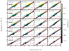 |
Fig. B.1. Same as Fig. 2, but showing in addition OLS bisector (solid red lines) and Bayesian fits (dash-dotted black lines) for comparison. The corresponding OLS bisector best-fit values for the slope, a, and the standard deviation of residuals, σ, are shown in the bottom-right corners of each panel. |
As highlighted above, all three explored fitting methods lead to different values for slope and dispersion around the best fit, which are systematically higher for the bisector OLS method compared to the standard OLS and Bayesian fits. However, qualitatively, the trends are similar at all redshifts and stellar mass bins.
B.2. Integrated KS
Figure B.3 is equivalent to Fig. 3, but showing the results of the OLS bisector fit (solid red lines), together with its best-fit values that can be compared to the Bayesian fit (dash-dotted black lines). As in the case of individual stellar mass bins, trends for the best-fit values of slope and dispersion around the best-fit stay qualitatively similar among all three fitting methods when stacking all galaxies at a given redshift. Quantitatively, the largest values of slope and dispersion around the best fit are again obtained for the OLS bisector method.
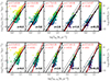 |
Fig. B.3. Same as Fig. 3, but showing in addition OLS bisector (solid red lines) and Bayesian (dash-dotted black lines) fits for comparison. The corresponding OLS bisector for the slope, a, and the standard deviation of residuals, σ, are shown in the bottom-right corners of each panel. |
B.3. Emergence of the KS relation
Figures B.4 and B.5 are the same as Figs. 4 and 5, but for the slopes and dispersions around the best-fit relation using the OLS bisector technique. As highlighted throughout this section, different fitting methods lead to quantitative differences in terms of values of the derived best-fit slope and dispersion around the best fit; however, qualitatively, the trends are recovered. This is clear from the comparison of Figures B.4 and B.5, adopting the OLS bisector method and Figures 4 and 5 of the main text using the Bayesian technique.
To conclude, our analysis reveals that the choice of the fitting method impacts the quantitative conclusions for all the measurements and diagnostics presented, but that the overall qualitative trends hold.
Appendix C: Deprojected KS relation
Figure C.1 displays the dependence of molecular gas fraction(top row), the neutral gas fraction (middle row), and Mach number (bottom row) of galaxies at different redshifts (columns) on the MH2-SFR plane. The trends seen for the projected quantities ΣH2 and ΣSFR are reproduced; in other words, the only physical parameter that evolves with both ΣH2 and ΣSFR is the Mach number, ℳ.
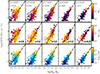 |
Fig. C.1. Same as Fig. 9, but color-coded by the molecular gas mass over the total neutral mass (top row), i.e., MH2/(MH I + MH2), the neutral baryonic gas fraction (middle row), i.e., (MH I + MH2)/MH I + MH2 + M⋆), and the Mach number (bottom row). For comparison, dotted-dash lines correspond to the OLS bisector fits. The corresponding best-fit values for the slope, a, and the standard deviation of residuals, σ, are shown in the top-left corners of each panel. |
We find that the results identified in the projected (i.e., observable) versions of the KS plane are also present in their deprojected counterparts, which means that our conclusions are not affected by projection artifacts.
All Tables
Number of galaxies and median of their stellar mass (in log M⊙) used in our analysis, at each redshift.
All Figures
|
Fig. 1. Projection of gas density, within the 10 Reff thick slices, of representative galaxies at different redshifts (rows) and stellar masses (columns). Dashed circles show the effective radius of the stellar component (see Sect. 2.2 for the definition), and the white horizontal bars indicate a 1 kpc scale. |
| In the text | |
|
Fig. 2. Distribution of galaxies in the KS plane at different redshifts (rows) and in four equally populated stellar mass quartiles at each redshift (columns). The mass range of each quartile is shown in square brackets (in log M⊙). The colors indicate the sSFR of the galaxies, measured over a timescale of 10 Myr. Dash-dotted lines are fits at each redshift and mass bin, with the slopes (a) and the standard deviation of residuals of the best-fit relation (σ) shown in the lower-right corners. The coefficient R, shown at the bottom right of each panel, is the Pearson correlation coefficient. The solid black and dotted black lines show the sequence of disks and starbursts, respectively, from Daddi et al. (2010) for reference. Note, however, that our fitting method differs from theirs. Regardless of stellar mass, the distributions of galaxies move within the KS plane toward lower values of ΣH2 and ΣSFR with decreasing redshift. At each redshift and in each stellar mass bin, the sSFR of galaxies strongly correlates with ΣSFR. Figure A.1 shows the same but using the neutral gas. |
| In the text | |
|
Fig. 3. Same as Figs. 2 and A.1, but without binning the stellar masses, and considering the molecular gas only (top) and the neutral gas (bottom). The correlation between the sSFR and ΣSFR seen in different stellar mass bins (Fig. 2) is still apparent when stacking all galaxies. At all redshifts, the slope (a) and the dispersion (σ) around the best-fit relation (dash-dotted line) are larger for the neutral gas than for the molecular gas. At all redshifts, the correlation is stronger for molecular gas than for neutral gas. |
| In the text | |
|
Fig. 4. Evolution of the slope of the fits of the KS relation from Figs. 2 and A.1, i.e., using the Bayesian fitting method, for the four mass bins considered, from the low-mass bin in a light color to the most massive one in a dark color. The red points show the slope of the entire galaxy population at a given redshift (i.e., without accounting for their mass, as in Fig. 3). After z ≈ 2 − 3, the slope of the KS relation for the two most massive bins remains within 30% (respectively 37%) of its final, converged, value for the molecular (respectively neutral) gas, which indicates the emergence of the KS relation at these redshifts. Low-mass galaxies do not show signs of convergence toward a fixed slope: their KS relation gets continuously shallower after z ≈ 2 − 3. |
| In the text | |
|
Fig. 5. Same as Fig. 4, but showing the dispersion around the best fit. Only the vertical dispersion, i.e., in log(ΣSFR), is considered here. |
| In the text | |
|
Fig. 6. Same as Fig. 3, but color-coded by the molecular over cold gas fraction (top), and baryonic molecular (middle) and neutral (bottom) gas fractions. The molecular gas fraction (top panel) correlates with ΣH2 at all redshifts. The baryonic molecular fraction (middle panel) correlates with ΣH2 at high redshifts; below z ∼ 2 this correlation weakens and is essentially carried by low-mass galaxies. The correlation between the neutral gas fraction and ΣH2 is apparent only at z = 4. At z ≲ 2 the trend reverses, meaning this fraction decreases with increasing ΣH2. |
| In the text | |
|
Fig. 7. Same as Fig. 3, but color-coded by the Mach number, ℳ. At all redshifts, ℳ increases monotonically with both increasing ΣH2 and ΣSFR. At fixed ΣH2, ℳ is correlated with ΣSFR. |
| In the text | |
|
Fig. 8. Normalized distributions of gas velocity dispersion (left), temperature (middle), and Mach number (right) in different stellar mass bins (colored lines, as indicated in the legend, report the logarithm of M⋆ in units of M⊙) and redshifts (indicated in the upper-left part of each panel). Vertical lines represent medians of distributions. |
| In the text | |
|
Fig. 9. Distribution of galaxies in the MH2–SFR plane, i.e., a deprojected version of the KS plane, at redshifts 4, 3, 2, 1, and 0.25, from left to right, as a function of galaxy mass (top) and effective radius (bottom). Dash-dotted lines are fits in the logarithmic space at each redshift, with the slope, a, and the standard deviation of residuals, σ. The coefficient R is the Pearson correlation coefficient. At all redshifts, more massive galaxies tend to have higher SFRs and MH2 values compared to their lower-mass counterparts. As galaxies grow in mass, they also grow in size; however, no obvious correlation is seen between Reff, the SFR, and the molecular gas mass. |
| In the text | |
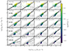 |
Fig. A.1. Same as Fig. 2, but for the neutral gas surface density ΣH I+H2. |
| In the text | |
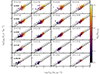 |
Fig. A.2. Same as Fig. 2, but color-coded by the molecular over cold gas fraction. |
| In the text | |
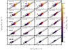 |
Fig. A.3. Same as Fig. 2, but color-coded by the baryonic molecular gas fraction. |
| In the text | |
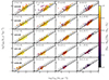 |
Fig. A.4. Same as Fig. 2, but color-coded by the neutral gas fraction. |
| In the text | |
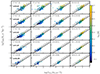 |
Fig. A.5. Same as Fig. 2, but color-coded by the Mach number. |
| In the text | |
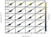 |
Fig. A.6. Same as Fig. 2, but color-coded by the gas velocity dispersion. |
| In the text | |
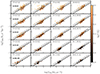 |
Fig. A.7. Same as Fig. 2, but color-coded by the gas temperature. |
| In the text | |
|
Fig. B.1. Same as Fig. 2, but showing in addition OLS bisector (solid red lines) and Bayesian fits (dash-dotted black lines) for comparison. The corresponding OLS bisector best-fit values for the slope, a, and the standard deviation of residuals, σ, are shown in the bottom-right corners of each panel. |
| In the text | |
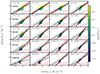 |
Fig. B.2. Same as Fig. B.1, but for the neutral gas surface density, ΣH I+H2. |
| In the text | |
|
Fig. B.3. Same as Fig. 3, but showing in addition OLS bisector (solid red lines) and Bayesian (dash-dotted black lines) fits for comparison. The corresponding OLS bisector for the slope, a, and the standard deviation of residuals, σ, are shown in the bottom-right corners of each panel. |
| In the text | |
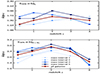 |
Fig. B.4. Same as Fig. 4, but using the OLS bisector fitting method (values from Figs. B.1 and B.2). |
| In the text | |
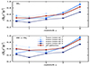 |
Fig. B.5. Same as Fig. 5, but using the OLS bisector fitting method (values from Figs. B.1 and B.2). |
| In the text | |
|
Fig. C.1. Same as Fig. 9, but color-coded by the molecular gas mass over the total neutral mass (top row), i.e., MH2/(MH I + MH2), the neutral baryonic gas fraction (middle row), i.e., (MH I + MH2)/MH I + MH2 + M⋆), and the Mach number (bottom row). For comparison, dotted-dash lines correspond to the OLS bisector fits. The corresponding best-fit values for the slope, a, and the standard deviation of residuals, σ, are shown in the top-left corners of each panel. |
| In the text | |
Current usage metrics show cumulative count of Article Views (full-text article views including HTML views, PDF and ePub downloads, according to the available data) and Abstracts Views on Vision4Press platform.
Data correspond to usage on the plateform after 2015. The current usage metrics is available 48-96 hours after online publication and is updated daily on week days.
Initial download of the metrics may take a while.