| Issue |
A&A
Volume 682, February 2024
|
|
|---|---|---|
| Article Number | A87 | |
| Number of page(s) | 9 | |
| Section | The Sun and the Heliosphere | |
| DOI | https://doi.org/10.1051/0004-6361/202346898 | |
| Published online | 06 February 2024 | |
Solar cycle variation in the properties of photospheric magnetic concentrations
1
Deep Space Exploration Laboratory/School of Earth and Space Sciences, University of Science and Technology of China, Hefei 230026, PR China
e-mail: This email address is being protected from spambots. You need JavaScript enabled to view it.
2
CAS Center for Excellence in Comparative Planetology/CAS Key Laboratory of Geospace Environment/Mengcheng National Geophysical Observatory, University of Science and Technology of China, Hefei 230026, PR China
3
Hefei National Laboratory, University of Science and Technology of China, Hefei 230088, PR China
4
Collaborative Innovation Center of Astronautical Science and Technology, Hefei 230026, PR China
5
School of Space and Environment, Beihang University, Beijing 100191, PR China
Received:
12
May
2023
Accepted:
16
November
2023
Abstract
It is widely accepted that eruptive phenomena on the Sun are related to the solar magnetic field, which is closely tied to the observed magnetic concentrations (MCs). Therefore, studying MCs is critical in order to understand the origin and evolution of all forms of solar activity. In this paper, we investigate the statistics of characteristic physical parameters of MCs during a whole solar cycle by analyzing magnetograms from 2010 to 2021 observed by the Helioseismic and Magnetic Imager (HMI) on board the Solar Dynamics Observatory (SDO). We discover that there are differences between large- and small-scale MCs in diffenent phases of the solar cycle. By analyzing the distributions of the magnetic flux, area, and magnetic energy of MCs, we find that the small-scale MCs obey a power-law distribution, and that the power indices vary very little with the phases of the solar cycle. However, for the large-scale MCs, although they also obey the power-law distribution, the power indices are clearly modulated by the different phases of the solar cycle. We also investigate the relation between the maximum magnetic field strength (Bmax) and the area of MCs (S) and find the same property. The relation for the large-scale MCs is modulated by the phases of the solar cycle, while it is still independent of the phases of the solar cycle for the small-scale MCs. Our results suggest that small- and large-scale MCs could be generated by different physical mechanisms.
Key words: Sun: magnetic fields / Sun: photosphere
© The Authors 2024
 Open Access article, published by EDP Sciences, under the terms of the Creative Commons Attribution License (https://creativecommons.org/licenses/by/4.0), which permits unrestricted use, distribution, and reproduction in any medium, provided the original work is properly cited.
This article is published in open access under the Subscribe to Open model. This email address is being protected from spambots. You need JavaScript enabled to view it. to support open access publication.
1. Introduction
Solar magnetic fields are closely related to various kinds of solar activity (Moore et al. 2001; Javaherian et al. 2017). The magnetic fields originate from the Sun’s global dynamo (Hagenaar et al. 2003; Mackay & Yeates 2012; Charbonneau 2020) and are transported to the photosphere in the form of flux tubes, for example via magnetic emergence (Harvey & Martin 1973; Schrijver et al. 1997; Schrijver & De Rosa 2003; Thornton & Parnell 2011; Cheung & Isobe 2014). The flux tubes undergo a random walk (Jiang et al. 2014; Giannattasio et al. 2019; Giannattasio & Consolini 2021) and evolve into positive- and negative-polarity magnetic concentrations (MCs; Parnell 2002), Zwaan (1987), Solanki (1993). Understanding the temporal and spatial properties of MCs is crucial in order to comprehend the spatiotemporal variation of the solar magnetic field, which is a key factor in our understanding of the solar dynamo.
Statistical analysis is a vital tool in the investigation of MCs and has been extensively used in previous studies (Lin 1995; Schrijver et al. 1997; Hagenaar et al. 1997; Abramenko & Longcope 2005; Solanki et al. 2006; Canfield & Russell 2007; Tlatov & Pevtsov 2014; Javaherian et al. 2017), which mainly focus on the analysis of various parameters associated with MCs, including their magnetic flux, magnetic field strength, area, lifetime, and so on (Martin 1988; Lin 1995; Hagenaar et al. 1997; Zhang et al. 1998; Hagenaar 2001; Parnell 2002; Tlatov & Pevtsov 2014; Muñoz-Jaramillo et al. 2015; Jin & Wang 2015). These parameters may all be used to estimate the features of an MC (Sheeley 1966; Harvey & Martin 1973; Spruit 1981; Lin 1995; Hagenaar et al. 1999; Hagenaar 2001; Parnell 2001, 2002; Cameron & Schüssler 2015; Muñoz-Jaramillo et al. 2015). It is revealed that MCs have a wide range of fluxes and areas (Solanki et al. 2006), ranging from the largest MCs, called sunspots, which have areas of 2 × 1019 cm2 and fluxes of several 1022 Mx, to the smallest MCs, which are inter-network magnetic fields, and have areas of just 1014 cm2 (Stenflo 1973) and fluxes of the order 1016 Mx (Parnell et al. 2009). MCs vary significantly across time and space; for example, the well-known 11 year solar cycle indicates that sunspot numbers fluctuate over 11 years (Muller & Roudier 1994; Meunier 2003; Hagenaar et al. 2003; Hathaway 2010, 2015; Muñoz-Jaramillo et al. 2015; Jin & Wang 2015; Gošić et al. 2016) and the butterfly diagram of sunspots indicates that sunspots move from mid-latitude to the equator over 11 years (Maunder 1904). However, in addition to sunspots that follow an 11 year cycle, there are also some magnetic structures described in previous works that have no association with – or a weaker dependence on – the solar cycle (Hagenaar et al. 2003; Karak & Brandenburg 2016; Rutten 2020; Wang et al. 2023). These structures may arise from surface turbulence dynamo (Cattaneo 1999; Sánchez Almeida et al. 2003; Pietarila Graham et al. 2010; Cameron & Schüssler 2015; Borrero et al. 2017; Rutten 2020). Therefore, the mechanism for generating the solar magnetic field is more complex and may require the coupling of multiple mechanisms.
It was suggested in the literature that the energy–frequency distribution of large- and small-scale MCs may be different. For instance, Meunier (2003) found that the distribution of small-area MCs follows a power law, while the distribution of large-area MCs deviates from this power law significantly. Similarly, Javaherian et al. (2017) found that the frequency of MC areas is best described by a broken double log–log linear function. However, Parnell et al. (2009) suggested that all MCs, regardless of their flux scale, follow a power-law distribution with an exponent of −1.85 based on observations from both the Michelson Doppler Imager (MDI, Scherrer et al. 1995) and the Solar Optical Telescope (SOT, Culhane et al. 2007). These discrepancies raise the significant question of whether small-scale and large-scale MCs are modulated by the same or different physical mechanisms.
Due to limitations in instrument observation duration and spatial resolution, previous statistical studies have rarely investigated MCs over a complete solar cycle with high-resolution data. Investigating MCs at the solar-cycle scale should help us to better understand their behavior and the underlying physical mechanisms leading to their production. Since 2010, the Solar Dynamics Observatory (SDO)/Helioseismic and Magnetic Imager (HMI, Schou et al. 2012) has been in operation, and has accrued over 11 years of data, allowing the investigation of MCs in a complete solar cycle with high spatial resolution and high signal-to-noise ratio (S/N). In this study, we used high-spatial-resolution magnetograms obtained by SDO/HMI from 2010 to 2021 to investigate the parametric characteristics of MCs, especially the variation of the distributions of the physical parameters of MCs in different phases of the solar cycle.
The rest of this paper is arranged as follows. The data and methods used in this study are described in Sect. 2. In Sect. 3, we investigate the properties of MCs, analyze their variation with respect to the solar cycle, and explore the relationship between the area of MCs and the magnetic field strength within them. Our findings are summarized and discussed in Sect. 4.
2. Data sets and data processing
2.1. Data sets
SDO/HMI (Scherrer et al. 2012) observations use the Fe I 6173 Å spectral line to provide maps of the line-of-sight component of the magnetic field averaged over the resolution element (0.6 arcsec, Schou et al. 2012). We use photospheric magnetic field strength data observed by SDO/HMI from 2010 to 2021, which cover a complete 11 year solar cycle. The magnetogram has a pixel area of 0.6 × 0.6 arcsec2. To encompass an entire solar cycle while taking into consideration data volume and processing time, we chose June 1–15 and December 1–15 each year to represent the data for that year. We note that, the b-angle during the time periods we select is quite small (Zhao et al. 2012), but that this parameter has very little impact on our dataset, and the primary error in our data comes from the projection effects, which is fixed by the procedure introduced in Sect. 2.2.
Observations near the solar limb tend to be influenced by the spectropolarimetric sensitivity effect. To avoid the impact of this effect and to ensure data credibility, Meunier (2003) chose to consider MCs within a latitude range of 53°. Similarly, Hagenaar et al. (2003) and Parnell et al. (2009) adopted a latitude range of 60° for MC selection. Following the results of these authors and considering that sunspots are mainly distributed within latitudes from −50° to 50° (Hathaway 2015), we chose a latitude range of −50° to ∼50°. Meanwhile, a longitude range of 20° should be sufficient to completely cover an active region (Tang et al. 1984), and so we chose the longitude range of −10° to ∼10° as the region of interest (ROI), and we focus on the MCs within this region in the present paper. Furthermore, according to the solar rotation speed (Howard 1984), the ROI turns at least 20 deg every 36 h, and so we chose a 36 h interval so as to avoid counting MCs twice.
2.2. Method
Starting from the selected data, we use the Clumping method (Parnell 2002; Hagenaar et al. 2003; DeForest et al. 2007) to identify MCs automatically. To determine the threshold of the magnetic field noise that is needed in the Clumping method, we use all the pixels of the selected magnetograms and plot the distribution of magnetic field strength per pixel, which is shown as the black line (Bb) in Fig. 1. We assume that the data can be divided into Guassian noise (Parnell 2002; Mursula et al. 2021) and real data, and so we fit the distribution with a Guassian function (gray line Bg) to determine the noise level. The blue line in Fig. 1 shows the relative deviation defined as  . The magnitude of deviation rises with increasing magnetic field strength. Here we set the threshold as 20 Mx cm−2 and the corresponding relative deviation reaches 30%, meaning that the noise is sufficiently separated from the data, as shown by the blue dashed line in Fig. 1.
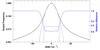 |
Fig. 1. Magnetic field strength per pixel distribution (black step-line Bb) and Gaussian fitting line (gray line Bg). The blue line shows the relative deviation, which is defined as |

With the estimated threshold, we assigned the pixels of MCs that have absolute values of less than 20 Mx cm−2 a value of 0. We then used the IDL function erode with a kernel of 3 × 3 pixels – as suggested by Haralick et al. (1987) and Hagenaar et al. (2003) – to remove very small clusters and isolated pixels. The results of noise removal and the erode process are shown in Figs. 2a,b. Finally, we identifed the remaining clusters as MCs. After identification, we kept those MCs located within the ROI. For the MCs that fall on the boundary of the ROI, following DeForest et al. (2007), we calculated their flux-weighted center (⟨Φdx⟩,⟨Φdy⟩) and discarded those whose centers are located outside of the ROI. The identification process and result are shown in Fig. 2c. The region outlined in red is the same as that shown in Fig. 3a. Using the method, we obtained 199 810 MCs after processing the data from 2010 to 2021. Table 1 provides details of the data.
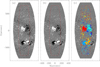 |
Fig. 2. Demonstration of the procedure used to identify MCs. The magnetogram is a cut-out from the magnetogram of Fig. 3a. The same region is marked by the red lines as in Fig. 3. From panel a to panel b we show the processes of noise removal and the erode method in the clumping method. Panel c shows the identified MCs from panel b. All MCs have been colored (positive MCs: warm tones; negative MCs: cold tones). |
Number of MCs during the different phases of the solar cycle.
Additionally, as suggested by Hagenaar et al. (2003), the observed line-of-sight component flux density ϕ(θ, λ) is the projection of the intrinsic flux density, ϕ⊥. Here, ϕ⊥ should be perpendicular to the solar surface, meaning that
 (1)
(1)
where the angles θ and λ are the latitude and longitude for each point (x, y) on the disk. The above equation was employed to correct the observed flux density to the intrinsic flux density. Similarly, we applied the same treatment  to the areas corresponding to pixels in the magnetograms to obtain the area of the solar surface.
3. Results
3.1. Distribution of parameters
Using the obtained MC data sets, we performed a statistical study of the distribution characteristics of the physical parameters of the MCs, including three parameters: the total magnetic flux (Φ), area (S), and energy  . First, we divided the detected MCs into two groups based on their polarities. The distributions of Φ for positive and negative MCs are illustrated by red and blue step lines in Fig. 4a1, respectively. Here, the distribution frequency is normalized by the maximum frequency. The distribution curves of positive and negative MCs appear almost identical, and we carried out a Kolmogorov–Smirnov two-sample test in order to verify that the two distributions curves are identical; the significance level exceeds 0.99, and therefore we suggest the two distribution curves are similar. The distributions of S and E for positive and negative MCs are shown in panels b1 and c1. Similarly, the Kolmogorov–Smirnov test significance level of the distributions curves of these parameters for positive and negative MCs are greater than 0.99. This indicates that the distributions of the studied characteristic parameters for the positive and negative MCs are similar. Therefore, positive and negative MCs are combined in the following analysis rather than separated.
The fluctuations in solar activity over the course of the complete solar cycle could be measured in terms of the day-averaged sunspot numbers, which are shown in Fig. 3b and are represented by a solid circle. The day-averaged sunspot numbers in each year were calculated with the observed sunspot numbers over the entire solar disk in June 1–15 and December 1–15 of each year. To further study the variation of MCs with the solar cycle, we divided the MCs into four parts based on the solar-cycle phase and day-averaged sunspots numbers with respect to our data sets: 2010–2011 and 2021 (ascending phase), 2012–2014 (maximum phase), 2015–2017 (declining phase), and 2018–2020 (minimum phase). The different phases are labeled with different colors in Fig. 3b: yellow for ascending phase, deep red for maximum phase, blue for declining phase, and dark blue for minimum phase. The corresponding day-averaged sunspot numbers during the four phases are 48.1, 98.3, 35.6, and 8.6, respectively, which were the average number of sunspots with the same color in Fig. 3b. The numbers of the recognized MCs in these four phases are listed in Table 1. The distributions of magnetic flux Φ, area S, and energy E for the different phases are depicted in Figs. 4a2–c2, where the ascending, maximum, declining, and minimum phases are represented by yellow, deep red, blue, and dark blue colors, respectively. As shown in Fig. 4a2, the distribution of Φ can be roughly divided into two sections. The distribution of Φ for the different solar-cycle phases is nearly identical for MCs with small Φ, indicating that the distributions of the parameters of the MCs with small Φ should vary very little during the solar cycle. Indeed, the results of a Kolmogorov–Smirnov two-sample test show that the four distribution curves of the parameters of the MCs are identical: the minimum significance level exceeds 0.98 in each case. However, when Φ is large, there are significant differences in the distributions of Φ for MCs in different solar-cycle phases: curves become steeper from maximum phase (deep red), to ascending phase (yellow), to declining phase (blue), and then to minimum phase (dark blue). The Kolmogorov–Smirnov test significance level of the four distribution curves gives a minimum value of less than 0.2, confirming that the distributions of the parameters of the MCs with large Φ are different. The critical values that divided the distribution curves into two sections is approximately Φc = 5.5 × 10¹⁸ Mx, as shown by the red dashed line in Fig. 4a2. We call this kind of distribution a “two-segment” power-law distribution. To quantitatively study the differences between the distributions of the physical parameters of MCs with small and large Φ, we performed a power-law fit of the distribution curves of small and large Φ, considering that the distribution of the physical parameters of MCs was frequently described as a power-law distribution in earlier investigations (Das & Das Gupta 1982; Tang et al. 1984; Hagenaar 2001; Parnell 2002; Meunier 2003; Hagenaar et al. 2003; Parnell et al. 2009, 2014; Thornton & Parnell 2011; Iida 2012; Javaherian et al. 2017). For small Φ MCs, we fit their distribution curves for different phases separately, and the power indices for the maximum phase, ascending phase, declining phase, and minimum phase are −1.58, −1.64, −1.63, and −1.71, respectively. Similarly, we estimate the power-law indices for S and E, and the relationship between the indices and the average sunspot numbers are plotted in Fig. 5a, where the solid triangle denotes Φ, the solid diamond denotes S, and the solid circle denotes E. The figure shows that there might be almost no relationship between the power indices of the physical parameters of the small-scale MCs and the sunspot numbers. This suggests that the physical parameters of small-scale MCs could be largely independent of the solar cycle. This result is consistent with the recent findings of Wang et al. (2023), who show that active regions with weaker flux have a weaker cycle dependence. Furthermore, as the distributions of small-scale MCs for different phases are close to each other, we also try to fit them together and obtain a power index of −1.64, as shown by the gray dashed line in Fig. 4a2.
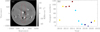 |
Fig. 3. Magnetograms and averaged sunspot number. Panel a: photospheric solar disk magnetic field observation by HMI on 2 December 2014 12:00:00. The color represents the strength of magnetic field. The region marked by the red lines shows −50° to ∼50° in latitude and −10° to ∼10° in longitude. Panel b: day-averaged sunspot numbers in each year during the time of data sets. The colors represent the phases: Yellow for ascending phase, deep red for maximum phase, blue for declining phase, and dark blue for minimum phase. |
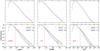 |
Fig. 4. Histogram of the physical parameters of the MCs in our data set. The parameters from left to right are magnetic flux (Φ), area (S), and magnetic energy (E). Top (a1, b1, c1): red line represents the distributions of positive MCs and blue line represents distributions of negative MCs. Bottom (a2, b2, c2): distributions of parameters corresponding to different phases in the solar cycle. The curves corresponding to different phases are signed with different colors. For the ascending, maximum, declining, and minimum phases, the corresponding colors are yellow, deep red, blue, and dark blue. The gray dashed line shows the power-law fitting of the distributions of the parameters of the MCs with small parameters. Dashed colored lines show power-law fits to the distributions of the parameters of the MCs with large parameters in different phases. The power index for each phase is given in the legend. The red dashed line indicates the broken point. |
For MCs with large Φ, we fit the distribution curves for each of the physical parameters for the different phases separately, and the fitting results are shown in Fig. 4 by the dashed lines colored according to solar-cycle phase. The power indices for the maximum phase, ascending phase, declining phase, and minimum phase are −1.92, −1.99, −2.07, and −2.27, respectively. We plot the obtained power indices for the four phases as a function of the average sunspot number during the corresponding phases, and the error bars represent the 1σ fitting error, which is shown in Fig. 4. The graph shows a clear positive correlation between power index and sunspot number, with a Pearson correlation coefficient of around 0.91. This suggests that the solar cycle has a significant influence on the distributions of the physical parameters of MCs with large Φ. Our analysis of S and E yields similar results: the distributions of MCs with small S and small E vary very little with solar-cycle phase, while the distributions of MCs with large S and large E exhibit significant differences between different solar-cycle phases. The critical values of S and E are: Sc = 5.5 ppm (millionths of a solar disk) and Ec = 3 × 10¹⁴ J. Similarly, we estimate the power-law indices for S and E, as displayed in Figs. 4b2 and c2, and the relationship between index and average sunspot number is plotted in Fig. 5b, where the solid diamond denotes S and the solid circle denotes E. The correlation coefficients between the power-law indices and the sunspot numbers are separately calculated, and the results for S and E are 0.91 and 0.9, respectively, indicating that the solar cycle also greatly modulates the MCs with large S and large E.
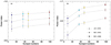 |
Fig. 5. Relationship between sunspot number and power index of the physical parameters of MCs. Panel a: power indices of the physical parameters of small-scale MCs. Panel b: power indices of the physical parameters of large-scale MCs; the power indices are the same as those in Fig. 4. |
The different varying trends of the distributions of the physical parameters of the large- and small-scale MCs with the solar cycle are consistent with the explanation that these two groups of MCs are generated by different mechanisms.
3.2. Relationships between parameters
The magnetic field distribution within an MC is often considered as a two-dimensional Gaussian distribution (Meyer et al. 2011; Meyer & Mackay 2016), which is controlled by two parameters: the maximum magnetic field strength Bmax ≡ MAX{B} and the area S of the ME. This implies that the relationship between these two characteristics is also critical for comprehending the ME. The distributions of the number density of MCs in the phase space of Bmax and S are shown in Figs. 6a1–a4, which depict the number densities of MCs in ascending, maximum, declining, and minimum phases, respectively. The number density of the contours increases from the outside to the interior. To quantify the association between Bmax and S, we split the MCs into 20 groups based on the value of S, with each group containing the same number of MCs, and then compute the median Bmax for each group and highlight it with an asterisk in Figs. 6a1–a4. The relationship between the median of Bmax and S can be fitted by a square-root function:
 (2)
(2)
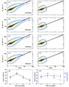 |
Fig. 6. Relationships between S and Bmax of MC. Panel a1, a2, a3, a4: number density of MCs in Bmax and S space in different solar-cycle phases. The contour lines correspond to 3, 15, 30, 150, 300, and 450 MCs. The black line shows the square-root fit. Panel a5: square-root fit coefficient α versus sunspot number. The blue dashed line shows sunspot numbers. The Φ of MCs in panels b1, b2, b3, b4, and b5 is less than 5.5 × 10¹⁸ Mx. |
where α and β are the fitting coefficients. Clearly, larger α represents a steeper curve, meaning that the Bmax of an MC is more likely to be larger. The black solid line in Fig. 6 represents the fitted curve. We examine the fitted coefficient α versus the sunspot numbers for different phases, as plotted by the cross symbols in Fig. 6a5, and blue circles denote the corresponding sunspot numbers. A strong correlation is clearly seen between sunspot number and α. As a result, the connection between Bmax and S of MCs correlates to the solar cycle and the fitting coefficient α may be used as a proxy for solar activity.
As concluded in Sect. 3.1, small-scale MCs are not modulated by the solar cycle. Here, we further examine the correlation between Bmax and S for small-scale MCs at various solar cycle phases. We filter out the MCs with Φ smaller than Φc = 5.5 × 10¹⁸ Mx and perform a similar analysis on them. The result are shown in panels b1–b4 of Fig. 6. Similarly, we divide these MCs into ten groups according to the values of S, with the same number of MCs in each group, and we obtain the median Bmax for each group. We fitted the meridian Bmax using Eq. (2), and the fitting coefficients α are plotted in panel b5 along with the sunspot numbers at different solar-cycle phases. The figure shows that the relationship between Bmax and S of MCs with small Φ scarcely varies with solar-cycle phase. These results further confirm that small-scale MCs are independent of the solar cycle.
4. Conclusion and discussion
We analyzed the magnetic field data over a 12 year period from 2010 to 2021, and extracted MCs using an automatic identification method. We used these data to study the evolutionary characteristics of the physical parameters of MCs with respect to the solar cycle. Our main results can be summarized as follows:
-
The distributions of the magnetic flux Φ, area S, and magnetic energy E for positive- and negative-polarity MCs are very similar.
-
MCs with different parameters can be divided into two groups based on their parameter values. During the solar cycle, these two groups display differing evolutionary traits. Both groups follow power-law distributions, but the power index for small-scale MCs is almost constant over the different phases of the solar cycle, while it varies considerably for large-scale MCs. The corresponding sunspot numbers and the power-law indices of the larger-scale MCs throughout various solar-cycle phases are strongly correlated. The critical values that distinguish the two groups: magnetic flux Φc = 5.5 × 10¹⁸ Mx, area Sc = 5.5 ppm, and magnetic energy Ec = 3 × 10¹⁴ J.
-
The maximum magnetic field strength (Bmax) of MCs is correlated with their area (S), and the dependence of Bmax on S changes with the solar-cycle phase.
These results show that the solar cycle has little bearing on the distributions of the physical parameters of small-scale MCs, meaning that small-scale MCs are likely generated by physical mechanisms unrelated to the solar cycle. On the other hand, the distributions of the physical parameters of large-scale MCs are greatly influenced by the solar cycle, which raises the possibility that large-scale MCs are generated by physical mechanisms related to the solar cycle.
In previous analyses of MCs parameters, most studies analyzed all scales of MCs together. Our results imply that the properties of small-scale and large-scale MCs with respect to the solar cycle differ significantly, and as a result, should be studied individually. This result suggests that a two-segment power-law may be more appropriate for investigating the frequency distributions of the physical parameters of MCs. According to our findings, the critical values of Φc, Sc, and Ec are all significantly lower than the typical scale of active regions and reach the scales of the network magnetic field. This suggests that in our MC data set, in addition to sunspots and active regions, some magnetic features on the quiet Sun, such as network magnetic field, are also modulated by the solar cycle. As introduced in Sect. 1, the magnetic field generated by the global dynamo exhibits an 11 year cycle, while the magnetic field produced by surface turbulent dynamo should hardly be related to the solar cycle. We therefore propose that small-scale MCs, which show almost no variation with the solar cycle, may originate from the surface turbulent dynamo, while the large-scale MCs strongly correlated with the solar cycle may be generated by the global dynamo.
As introduced in Sect. 2.2, the Clumping method involves the use of a threshold, and it seems that the threshold may have some influence on the statistical results of MCs. Many previous studies questioned the effect of this threshold value on the results of the Clumping method. For example, Meunier (2003) discussed the impact of the threshold on MC identification and found that the conclusions remained consistent regardless of whether the threshold was set at 25 G or 40 G. To assess the impact of threshold values on our results, we adjusted the thresholds and repeated the analyses of this paper; the results are presented in Appendix A. Although, the threshold used in the Clumping method could result in a reduced number of identified small-scale MCs (Parnell et al. 2009) and different threshold values could lead to variations in the identification number of small-scale MCs, we find that the statistical results remain similar, which is consistent with Meunier (2003). This suggests that the selection of threshold values has little influence on the conclusions of our study.
We note in Fig. 6 that the Bmax of the MCs saturates at large values of S, and we posit that this saturation may be caused by the filling factor of the magnetic field. Parnell et al. (2009) proposed that small MCs have narrower magnetic flux tubes than large MCs. Therefore, the observed magnetic flux density is smaller than the actual magnetic field strength inside the flux tube at small sizes because the filling factor is less than 1. As the scale grows, the filling factor also grows. When the scale of ME reaches the size of a sunspot, the filling factor approaches 1, resulting in an observed magnetic flux density equivalent to the actual magnetic field intensity within the flux tube, which is ∼1000 G. This phenomenon explains the finding that Bmax rapidly grows when S is small, and saturates at ∼1000 G when S is big. Also, in addition to the saturation of Bmax at high values of S, we observe a lower cutoff of Bmax, which means there are no MCs with large S but small Bmax. The mechanism behind this phenomena is unknown. Further research will be needed to fully understand the physical causes. In future work, we plan to use data observed by satellites, such as the Space-based Solar Observatory (ASO-S, Gan et al. 2019), to further investigate MCs.
Acknowledgments
We appreciate the reference provided by the anonymous reviewer. This research is supported by the National Natural Science Foundation of China (NSFC 42188101, 11925302, 42174213, 41804161), the Informatization Plan of Chinese Academy of Sciences, Grant No. CAS-WX2022SF-0103, the Key Research Program of the Chinese Academy of Sciences, Grant No. ZDBS-SSW-TLC00103, and the Innovation Program for Quantum Science and Technology(2021ZD0300302). This research is also supported by USTC Research Funds of the Double First-Class Initiative. The authors acknowledge for the support from National Space Science Data Center, National Science & Technology Infrastructure of China (www.nssdc.ac.cn). Quanhao Zhang acknowledge for the support from Young Elite Scientist Sponsorship Program by the China Association for Science and Technology (CAST).
References
- Abramenko, V. I., & Longcope, D. W. 2005, ApJ, 619, 1160 [NASA ADS] [CrossRef] [Google Scholar]
- Borrero, J. M., Jafarzadeh, S., Schüssler, M., & Solanki, S. K. 2017, Space Sci. Rev., 210, 275 [Google Scholar]
- Cameron, R., & Schüssler, M. 2015, Science, 347, 1333 [Google Scholar]
- Canfield, R. C., & Russell, A. J. B. 2007, ApJ, 662, L39 [NASA ADS] [CrossRef] [Google Scholar]
- Cattaneo, F. 1999, ApJ, 515, L39 [Google Scholar]
- Charbonneau, P. 2020, Liv. Rev. Sol. Phys., 17, 4 [Google Scholar]
- Cheung, M. C. M., & Isobe, H. 2014, Liv. Rev. Sol. Phys., 11, 3 [Google Scholar]
- Culhane, J. L., Harra, L. K., James, A. M., et al. 2007, Sol. Phys., 243, 19 [Google Scholar]
- Das, T. K., & Das Gupta, M. K. 1982, Sol. Phys., 78, 67 [NASA ADS] [CrossRef] [Google Scholar]
- DeForest, C. E., Hagenaar, H. J., Lamb, D. A., Parnell, C. E., & Welsch, B. T. 2007, ApJ, 666, 576 [NASA ADS] [CrossRef] [Google Scholar]
- Gan, W.-Q., Zhu, C., Deng, Y.-Y., et al. 2019, RAA, 19, 156 [Google Scholar]
- Giannattasio, F., & Consolini, G. 2021, ApJ, 908, 142 [NASA ADS] [CrossRef] [Google Scholar]
- Giannattasio, F., Consolini, G., Berrilli, F., & Del Moro, D. 2019, ApJ, 878, 33 [NASA ADS] [CrossRef] [Google Scholar]
- Gošić, M., Bellot Rubio, L. R., del Toro Iniesta, J. C., Orozco Suárez, D., & Katsukawa, Y. 2016, ApJ, 820, 35 [Google Scholar]
- Hagenaar, H. J. 2001, ApJ, 555, 448 [NASA ADS] [CrossRef] [Google Scholar]
- Hagenaar, H. J., Schrijver, C. J., & Title, A. M. 1997, ApJ, 481, 988 [NASA ADS] [CrossRef] [Google Scholar]
- Hagenaar, H. J., Schrijver, C. J., Title, A. M., & Shine, R. A. 1999, ApJ, 511, 932 [CrossRef] [Google Scholar]
- Hagenaar, H. J., Schrijver, C. J., & Title, A. M. 2003, ApJ, 584, 1107 [NASA ADS] [CrossRef] [Google Scholar]
- Haralick, R. M., Sternberg, S. R., & Zhuang, X. 1987, IEEE Trans. Patt. Anal. Mach. Intell., 9, 532 [CrossRef] [Google Scholar]
- Harvey, K. L., & Martin, S. F. 1973, Sol. Phys., 32, 389 [NASA ADS] [CrossRef] [Google Scholar]
- Hathaway, D. H. 2010, Liv. Rev. Sol. Phys., 7, 1 [Google Scholar]
- Hathaway, D. H. 2015, Liv. Rev. Sol. Phys., 12, 4 [Google Scholar]
- Howard, R. 1984, ARA&A, 22, 131 [NASA ADS] [CrossRef] [Google Scholar]
- Iida, I. 2012, arXiv e-prints [arXiv:1212.6310] [Google Scholar]
- Javaherian, M., Safari, H., Dadashi, N., & Aschwanden, M. J. 2017, Sol. Phys., 292, 164 [NASA ADS] [CrossRef] [Google Scholar]
- Jiang, J., Hathaway, D. H., Cameron, R. H., et al. 2014, Space Sci. Rev., 186, 491 [Google Scholar]
- Jin, C., & Wang, J. 2015, ApJ, 806, 174 [NASA ADS] [CrossRef] [Google Scholar]
- Karak, B. B., & Brandenburg, A. 2016, ApJ, 816, 28 [Google Scholar]
- Lin, H. 1995, ApJ, 446, 421 [NASA ADS] [CrossRef] [Google Scholar]
- Mackay, D. H., & Yeates, A. R. 2012, Liv. Rev. Sol. Phys., 9, 6 [Google Scholar]
- Martin, S. F. 1988, Sol. Phys., 117, 243 [NASA ADS] [CrossRef] [Google Scholar]
- Maunder, E. W. 1904, MNRAS, 64, 747 [NASA ADS] [Google Scholar]
- Meunier, N. 2003, A&A, 405, 1107 [NASA ADS] [CrossRef] [EDP Sciences] [Google Scholar]
- Meyer, K. A., & Mackay, D. H. 2016, ApJ, 830, 160 [Google Scholar]
- Meyer, K. A., Mackay, D. H., van Ballegooijen, A. A., & Parnell, C. E. 2011, Sol. Phys., 272, 29 [NASA ADS] [CrossRef] [Google Scholar]
- Moore, R. L., Sterling, A. C., Hudson, H. S., & Lemen, J. R. 2001, ApJ, 552, 833 [Google Scholar]
- Muñoz-Jaramillo, A., Senkpeil, R. R., Windmueller, J. C., et al. 2015, ApJ, 800, 48 [Google Scholar]
- Muller, R., & Roudier, T. 1994, Sol. Phys., 152, 131 [NASA ADS] [CrossRef] [Google Scholar]
- Mursula, K., Getachew, T., & Virtanen, I. I. 2021, A&A, 645, A47 [NASA ADS] [CrossRef] [EDP Sciences] [Google Scholar]
- Parnell, C. E. 2001, Sol. Phys., 200, 23 [NASA ADS] [CrossRef] [Google Scholar]
- Parnell, C. E. 2002, MNRAS, 335, 389 [NASA ADS] [CrossRef] [Google Scholar]
- Parnell, C. E., DeForest, C. E., Hagenaar, H. J., et al. 2009, ApJ, 698, 75 [Google Scholar]
- Parnell, C. E., Lamb, D. A., & DeForest, C. E. 2014, AGU Fall Meeting Abstracts, 2014, SH34A-05 [Google Scholar]
- Pietarila Graham, J., Cameron, R., & Schüssler, M. 2010, ApJ, 714, 1606 [Google Scholar]
- Rutten, R. 2020, Solar Magnetic Variability and Climate, 29 [Google Scholar]
- Sánchez Almeida, J., Emonet, T., & Cattaneo, F. 2003, ApJ, 585, 536 [CrossRef] [Google Scholar]
- Scherrer, P. H., Bogart, R. S., Bush, R. I., et al. 1995, Sol. Phys., 162, 129 [Google Scholar]
- Scherrer, P. H., Schou, J., Bush, R. I., et al. 2012, Sol. Phys., 275, 207 [Google Scholar]
- Schou, J., Scherrer, P. H., Bush, R. I., et al. 2012, Sol. Phys., 275, 229 [Google Scholar]
- Schrijver, C. J., & De Rosa, M. L. 2003, Sol. Phys., 212, 165 [Google Scholar]
- Schrijver, C. J., Title, A. M., van Ballegooijen, A. A., Hagenaar, H. J., & Shine, R. A. 1997, ApJ, 487, 424 [Google Scholar]
- Sheeley, N. R., Jr 1966, ApJ, 144, 723 [NASA ADS] [CrossRef] [Google Scholar]
- Solanki, S. K. 1993, Space Sci. Rev., 63, 1 [Google Scholar]
- Solanki, S. K., Inhester, B., & Schüssler, M. 2006, Rep. Progr. Phys., 69, 563 [CrossRef] [Google Scholar]
- Spruit, H. C. 1981, in NASA Special Publication, ed. S. Jordan, 450, 385 [NASA ADS] [Google Scholar]
- Stenflo, J. O. 1973, Sol. Phys., 32, 41 [NASA ADS] [CrossRef] [Google Scholar]
- Tang, F., Howard, R., & Adkins, J. M. 1984, Sol. Phys., 91, 75 [NASA ADS] [CrossRef] [Google Scholar]
- Thornton, L. M., & Parnell, C. E. 2011, Sol. Phys., 269, 13 [Google Scholar]
- Tlatov, A. G., & Pevtsov, A. A. 2014, Sol. Phys., 289, 1143 [Google Scholar]
- Wang, R., Jiang, J., & Luo, Y. 2023, ApJS, 268, 55 [NASA ADS] [CrossRef] [Google Scholar]
- Zhang, J., Lin, G., Wang, J., Wang, H., & Zirin, H. 1998, Sol. Phys., 178, 245 [NASA ADS] [CrossRef] [Google Scholar]
- Zhao, J., Nagashima, K., Bogart, R. S., Kosovichev, A. G., & Duvall, T. L., Jr 2012, ApJ, 749, L5 [Google Scholar]
- Zwaan, C. 1987, ARA&A, 25, 83 [NASA ADS] [CrossRef] [Google Scholar]
Appendix A: Effect of the threshold used in the Clumping method
We adjusted the threshold value to 15G or 25G in order to monitor the effects of changes to this threshold in our analysis. First, the distributions of the MC parameters are plotted in Figure A.1. Panels (d), (e), and (f) represent Figure 4 (a2, b2, c2) in the paper, in which the threshold was set at 20G; panels (a), (b), and (c) depict the results when the threshold is adjusted to 15G; while the panels (g), (h), and (i) show the results with a threshold of 25G. We find that the parameter distributions obtained with different threshold values are similar: all of them could be fitted using the two-segment power-law function mentioned in the Section 3.1; the distributions of large-scale MCs always exhibit an obvious variation with the solar cycle, while the distribution of small-scale MCs remains almost unchanged with respect to the solar cycle.
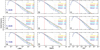 |
Fig. A.1. Distributions of parameters corresponding to different phases in the solar cycle. (a, b, c): The threshold value T = 25G. (d, e, f), (g, h, i): Same as (a, b, c), but for T = 20G and 15G, respectively. |
Second, the relationship between sunspot numbers and the power index of MC physical parameters is plotted in Figure A.2. Panel (b) shows the original Figure 5 (b) in the Section 4, while panels (a) and (c) depict the results obtained by modifying the threshold to 15G and 25G, respectively. With different threshold values, the power indices of large-scale MCs still exhibit a clear correlation with sunspot number, and the change in trend remains similar.
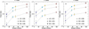 |
Fig. A.2. Relationship between sunspot number and power index of the physical parameters of large-scale MCs. (a): The threshold value T = 15G. Panels (b) and (c): Same as (a), but for T = 20G and 25G, respectively. |
Third, the coefficients corresponding to different threshold values are illustrated in Figure A.3. Panels (c) and (d)show the original Figure 6 (a5, b5), while panels (a) and (b) and panel (e) and (f) depict the results obtained by modifying the threshold to 15G and 25G, respectively. Similarly, for the cases with different threshold, the coefficients for all the MCs (left three panels) still exhibit a strong correlation with solar cycle, whereas those for the small-scale MCs (right three panels) are barely affected by the solar cycle.
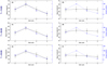 |
Fig. A.3. Square-root fit coefficient α versus sunspot number. (a, b): The threshold value T = 15G. (c, d) and (e, f): Same as (a, b), but for T = 20G and 25G, respectively. |
Therefore, as demonstrated above, the major conclusions in our paper are not influenced by the value of the threshold used in the Clumping method.
All Tables
All Figures
|
Fig. 1. Magnetic field strength per pixel distribution (black step-line Bb) and Gaussian fitting line (gray line Bg). The blue line shows the relative deviation, which is defined as |
| In the text | |
|
Fig. 2. Demonstration of the procedure used to identify MCs. The magnetogram is a cut-out from the magnetogram of Fig. 3a. The same region is marked by the red lines as in Fig. 3. From panel a to panel b we show the processes of noise removal and the erode method in the clumping method. Panel c shows the identified MCs from panel b. All MCs have been colored (positive MCs: warm tones; negative MCs: cold tones). |
| In the text | |
|
Fig. 3. Magnetograms and averaged sunspot number. Panel a: photospheric solar disk magnetic field observation by HMI on 2 December 2014 12:00:00. The color represents the strength of magnetic field. The region marked by the red lines shows −50° to ∼50° in latitude and −10° to ∼10° in longitude. Panel b: day-averaged sunspot numbers in each year during the time of data sets. The colors represent the phases: Yellow for ascending phase, deep red for maximum phase, blue for declining phase, and dark blue for minimum phase. |
| In the text | |
|
Fig. 4. Histogram of the physical parameters of the MCs in our data set. The parameters from left to right are magnetic flux (Φ), area (S), and magnetic energy (E). Top (a1, b1, c1): red line represents the distributions of positive MCs and blue line represents distributions of negative MCs. Bottom (a2, b2, c2): distributions of parameters corresponding to different phases in the solar cycle. The curves corresponding to different phases are signed with different colors. For the ascending, maximum, declining, and minimum phases, the corresponding colors are yellow, deep red, blue, and dark blue. The gray dashed line shows the power-law fitting of the distributions of the parameters of the MCs with small parameters. Dashed colored lines show power-law fits to the distributions of the parameters of the MCs with large parameters in different phases. The power index for each phase is given in the legend. The red dashed line indicates the broken point. |
| In the text | |
|
Fig. 5. Relationship between sunspot number and power index of the physical parameters of MCs. Panel a: power indices of the physical parameters of small-scale MCs. Panel b: power indices of the physical parameters of large-scale MCs; the power indices are the same as those in Fig. 4. |
| In the text | |
|
Fig. 6. Relationships between S and Bmax of MC. Panel a1, a2, a3, a4: number density of MCs in Bmax and S space in different solar-cycle phases. The contour lines correspond to 3, 15, 30, 150, 300, and 450 MCs. The black line shows the square-root fit. Panel a5: square-root fit coefficient α versus sunspot number. The blue dashed line shows sunspot numbers. The Φ of MCs in panels b1, b2, b3, b4, and b5 is less than 5.5 × 10¹⁸ Mx. |
| In the text | |
|
Fig. A.1. Distributions of parameters corresponding to different phases in the solar cycle. (a, b, c): The threshold value T = 25G. (d, e, f), (g, h, i): Same as (a, b, c), but for T = 20G and 15G, respectively. |
| In the text | |
|
Fig. A.2. Relationship between sunspot number and power index of the physical parameters of large-scale MCs. (a): The threshold value T = 15G. Panels (b) and (c): Same as (a), but for T = 20G and 25G, respectively. |
| In the text | |
|
Fig. A.3. Square-root fit coefficient α versus sunspot number. (a, b): The threshold value T = 15G. (c, d) and (e, f): Same as (a, b), but for T = 20G and 25G, respectively. |
| In the text | |
Current usage metrics show cumulative count of Article Views (full-text article views including HTML views, PDF and ePub downloads, according to the available data) and Abstracts Views on Vision4Press platform.
Data correspond to usage on the plateform after 2015. The current usage metrics is available 48-96 hours after online publication and is updated daily on week days.
Initial download of the metrics may take a while.