| Issue |
A&A
Volume 652, August 2021
|
|
|---|---|---|
| Article Number | A9 | |
| Number of page(s) | 6 | |
| Section | The Sun and the Heliosphere | |
| DOI | https://doi.org/10.1051/0004-6361/202140621 | |
| Published online | 02 August 2021 | |
On the size distribution of spots within sunspot groups
1
Max Planck Institute for Solar System Research, Justus-von-Liebig-Weg 3, 37077 Göttingen, Germany
e-mail: This email address is being protected from spambots. You need JavaScript enabled to view it.
2
School of Space Research, Kyung Hee University, 446-701 Yongin, Gyeonggi, Republic of Korea
Received:
21
February
2021
Accepted:
7
April
2021
Abstract
The size distribution of sunspots provides key information about the generation and emergence processes of the solar magnetic field. Previous studies of size distribution have primarily focused on either the whole group or individual spot areas. In this paper we investigate the organisation of spot areas within sunspot groups. In particular, we analysed the ratio (R) of the area of the biggest spot (Abig_spot) inside a group, to the total area of that group (Agroup). We used sunspot observations from Kislovodsk, Pulkovo, and Debrecen observatories, together covering solar cycles 17–24. We find that at the time when the group area reaches its maximum, the single biggest spot in a group typically occupies about 60% of the group area. For half of all groups, R lies in the range between roughly 50% and 70%. We also find R to change with Agroup, such that R reaches a maximum of about 0.65 for groups with Agroup ≈ 200 μHem and then remains at about 0.6 for larger groups. Our findings imply a scale-invariant emergence pattern, providing an observational constraint on the emergence process. Furthermore, extrapolation of our results to larger sunspot groups may have a bearing on the giant unresolved starspot features found in Doppler images of highly active Sun-like stars. Our results suggest that such giant features are composed of multiple spots, with the largest spot occupying roughly 55–75% of the total group area (i.e., the area of the giant starspots seen in Doppler images).
Key words: Sun: magnetic fields / sunspots / Sun: photosphere / Sun: activity
© S. Mandal et al. 2021
 Open Access article, published by EDP Sciences, under the terms of the Creative Commons Attribution License (https://creativecommons.org/licenses/by/4.0), which permits unrestricted use, distribution, and reproduction in any medium, provided the original work is properly cited.
Open Access funding provided by Max Planck Society.
1. Introduction
The magnetic field of the Sun, the driving force of its activity and variability, is generated in its interior by a dynamo action and emerges at the surface as bipolar regions. The larger of these regions typically host sunspots, which are dark photospheric features that trace the locations of highly concentrated magnetic field on the solar surface (Solanki 2003). Direct measurements of solar magnetic fields are only available for the last few decades, and hence sunspot area records, which have been observed more or less regularly over more than a century, act as a proxy of the surface magnetism and provide an indirect way of understanding the long-term behaviour of the magnetic activity and variability.
Sunspots usually emerge in groups, and within a typical group the spots are arranged into two sub-groups, leading (closer to the solar equator) and following. Spots in the leading sub-group are bigger and more coherent than those in the following sub-group (Bray & Loughhead 1979; McIntosh 1981). Although the reason behind such a configuration is not yet understood, it is believed to be related to the flux emergence process where various forces (e.g., Coriolis force, convective motions, sub-surface shears) act on a rising flux tube and determine its surface morphology (Borrero & Ichimoto 2011; van Driel-Gesztelyi & Green 2015).
One of the aspects that provides clues to understanding the processes of solar magnetic field generation and emergence is the size distribution of spots. Studies of the size distribution of the sunspot groups and the individual spots have been carried out in the past by various authors (Kuklin 1980; Bogdan et al. 1988; Baumann & Solanki 2005; Nagovitsyn et al. 2012; Tlatov & Pevtsov 2014; Muñoz-Jaramillo et al. 2015). Using the group area data from the Royal Greenwich Observatory (RGO), Bogdan et al. (1988) and Baumann & Solanki (2005) found that the size distribution, over most of its range, could be fairly well described by a log-normal function. Physically, a log-normal size distribution suggests that all spots are generated by a global dynamo action, with smaller spots being the fragmented products of the larger flux concentrations (Kolmogorov 1941). Later, Parnell et al. (2009) and Thornton & Parnell (2011) analysed various observations of the magnetic field emergence and concluded that they could all be described by a single power-law distribution covering seven orders of magnitude in flux. However, using individual spot area measurements from the Kislovodsk Mountain Station and group areas from RGO, Solar Observing Optical Network (SOON), Pulkovo, and Kislovodsk, Nagovitsyn et al. (2012) and Muñoz-Jaramillo et al. (2015) showed that the overall size distribution was better characterised by two separate distribution functions respectively for small and big groups or spots. They argued that such a bi-modal size distribution could possibly imply a more complex process of spot formation, for example driven by small-scale and global dynamos in parallel (Nagovitsyn & Pevtsov 2016). A similar conclusion was also reached by Tlatov & Pevtsov (2014), who analysed the magnetic flux and sunspot area records from Helioseismic and Magnetic Imager (HMI). However, results from recent high-resolution observations and numerical simulations suggest that the small-scale dynamo is mainly responsible for the generation of the (non-spot) weak fields (Pietarila Graham et al. 2010; Stenflo 2012; Rempel 2014; Karak & Brandenburg 2016).
Understanding the spot size distribution thus calls for further investigations. Furthermore, understanding the spot area distribution on the Sun can help us to understand the poorly known area distribution of starspots on other Sun-like stars (e.g., Solanki & Unruh 2004). In this paper we re-address the question of the size distribution of sunspots. However, instead of analysing the overall spot or group size distribution as was done in previous studies, here we focus on the distribution of spot areas within individual groups. We describe the data and the approach used in this study in Sect. 2 and the results in Sect. 3, while Sect. 4 summarises our conclusions.
2. Data and methods
We use sunspot area catalogues from three different sources, namely Debrecen Observatory1 (Baranyi et al. 2016; Győri et al. 2017), Kislovodsk Mountain station2 (Nagovitsyn et al. 2007), and Pulkovo observatory3 (Mikhailov 1955). The Kislovodsk (1954–2019) and Pulkovo (1932–1991) catalogues provide daily records of the total area of every individual group, Agroup (including umbrae and penumbrae), the total area of the biggest spot, Abig_spot (including umbra and penumbra), as well as the number, N, of individual umbrae in each group. Since some spots might include multiple umbrae (i.e., multiple umbrae embedded within the same penumbra; see Fig. 1), for some groups N can be higher than the number of the individual spots in the group. The Debrecen record is the official continuation of the RGO programme after it was ceased in 1976 (Baranyi et al. 2016). This catalogue4 lists daily measurements of Agroup and N values. Each spot in this catalogue carries a unique group label, using which we calculate Abig_spot from Debrecen as well.
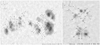 |
Fig. 1. Images of two sunspot groups (NOAA 7790 and NOAA 7680) from Debrecen observatory (These images are available at http://fenyi.solarobs.csfk.mta.hu/en/databases/DPD/). In each image individual umbrae are labelled with unique numbers. |
Since area measurements from different observatories show systematic differences (Fligge & Solanki 1997; Baranyi et al. 2001; Balmaceda et al. 2009), a cross-calibration is necessary before using them for any analysis. Various past studies have found that both the daily and the individual area measurements from the catalogues considered here (Deberecen, Kislovodsk, and Pulkovo) are very similar to each other, and also to the measurements from RGO, with mutual cross-calibration factors being close to unity (Nagovitsyn et al. 2007; Balmaceda et al. 2009; Baranyi et al. 2013; Muñoz-Jaramillo et al. 2015; Mandal et al. 2020). For the purpose of this work we use the latest calibration by Mandal et al. (2020) who compared these datasets statistically during the overlapping periods to generate a consistent and homogeneous area record.
To understand the area distribution of spots within individual groups, we focus on the biggest spot in the group and derive the ratio, R, between the area of the biggest spot and the total group area:
 (1)
(1)
According to this definition, the maximum possible value of R is 1, for groups with only one listed spot. We recall here that throughout this paper the term “spot” or “sunspot” refers to a structure that has a solitary umbra or multiple umbrae embedded within a single penumbra. All the areas used in this study are corrected for the foreshortening effect.
3. Results
3.1. Instantaneous distributions
We start by considering all data on every given day, i.e., irrespective of the group’s evolutionary phase on that day. The R values are then calculated for all individual group entries. Figure 2a shows the derived distributions of R from the Debrecen, Kislovodsk, and Pulkovo data. All three distributions display some common features: a sharp primary peak at R = 1 and a flatter secondary peak around R = 0.5. The peak at R = 1 comes from the single-spot groups for which Abig_spot = Agroup. These groups make up approximately 19% of all the listed entries in our catalogues. Since we are interested in the distribution of spots within a group, we remove these single-spot groups from our sample. In addition, we also reject small groups (areas less than 30 μHem) as they are likely to be associated with larger measurement uncertainties (see Muñoz-Jaramillo et al. 2015). We note, however, that a change in this threshold to different values within the range 30–80 μHem led to results that are only marginally different from those presented below, while reducing the statistics.
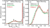 |
Fig. 2. Results from the instantaneous distribution analysis. Panel a: normalised distribution of R from Debrecen (black), Kislovodsk (green), and Pulkovo (red) when considering all daily individual groups, i.e., irrespective of their evolutionary phase. Panel b: same as panel a, but after removing groups with N = 1 and Agroup ≤ 30 μHem. |
The final distributions, after implementing these two restrictions, are shown in Fig. 2b. Two distinct features are evident in all three distributions. First, the distributions are clearly asymmetric, being skewed towards higher ratios (skewness = 0.03) and their mode values lying around R ≊ 0.5. Second, although the peak at R = 1 has now disappeared, a weak secondary peak is still seen at R ≊ 0.97, which is pronounced in the Debrecen and Pulkovo data and is significantly weaker in the Kislovodsk data. We return to this peak in Sect. 3.2.
The shape of these histograms might possibly be affected by the complex evolutionary scenarios of sunspot groups, such as fragmentation or coalescence (Schrijver et al. 1997). Furthermore, while spots emerge relatively fast, their decay times are much longer (Howard 1992). Thus, as has been pointed out in the past, the results derived from a snapshot distribution (i.e., considering all spots independently of their evolution) can potentially be dominated by the longer decay phase of sunspot groups (Baumann & Solanki 2005). To examine the influence of these effects on the obtained distributions, we track every group in our catalogues and re-derive the R distributions so that each group is considered only once.
3.2. Tracking individual sunspot groups
We first visually inspected a sub-set of Debrecen images5 from the period 1986–1999, which trace individual groups. These images are extractions of the full-disc photographs, and within each of these snapshots the spots forming a group are uniquely numbered. These images allowed us to trace 40 individual groups (chosen randomly). By following these groups from their first emergence to their disappearance, we noticed that, during the initial growth or final decay phase, the following spots are significantly smaller than the leading spots. In other words, as has also been noticed in earlier studies, leading spots form faster than the following ones (McIntosh 1981; Rempel & Cheung 2014) and decay more slowly that following spots (Bumba 1963). This leads to R values very close to (though not exactly) 1 during these periods. This is, in fact, the reason behind the weak secondary peak at R ∼ 0.97 that we see in the instantaneous distributions (Fig. 2b).
Therefore, we now use the information from all the catalogues considered here to track sunspot groups over their lifetimes. To minimise the errors introduced by the foreshortening corrections, only groups within central meridian distances of ±65°are considered here. Following the snapshot analysis described in the previous section, we leave out single-spot (N = 1) groups, and groups with areas less than 30 μHem. Our aim here is to consider every group only once over its entire lifetime. Usually, these studies consider the time when a group area reaches its maximum value. However, in our case the second parameter entering R, the size of the biggest spot also evolves with time and Abig_spot and Agroup do not necessarily reach their maximum at the same time. We find that only 65% of the total groups analysed here have the maximum of these two quantities on the same day. For 20% of all groups, Abig_spot reaches its maximum after the maximum in Agroup (termed a positive delay here) whereas 15% of the remaining groups show a negative delay. Both the positive and the negative delays mainly happen in big complex groups with many spots, which require a separate study. For the purpose of this paper, we only consider groups with no delay (i.e., when the groups and the biggest spot areas reach their maximum on the same day).
The distribution of R derived for these groups is shown in Fig. 3a. The maxima of the distributions in all three cases lie around R = 0.5 and, unlike the snapshot distributions, there are no secondary peaks. To further understand these distributions we calculate the quartiles Q1, Q2, and Q3, which describe the sample 25th, 50th, and 75th percentiles, respectively (Ross 2000) (see Table 1). In Fig. 3a the shaded regions highlight the quartiles computed for the distribution averaged over the three datasets. The range between Q1 and Q3 represents the interquartile range (IQR = Q3–Q1) where 50% of the data points around the median value (Q2) lie. The IQR is considered to be a measure of the spread of the distribution. For all the individual and the average distributions, the IQR is only 0.26. Such a low IQR indicates that the data are clustered about the central tendency (i.e., the median value (Q2) of R = 0.6). Thus, in the majority of groups, a single large spot occupies about 48–74% of the total group area.
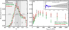 |
Fig. 3. Results from the tracked data. Panel a: normalised distribution of R calculated at the time of maximum Agroup. Panel b: R as a function of Agroup. The error bars represent the standard deviations calculated for each bin. Panel c: same as panel b, but averaged over the three individual datasets. The dashed line is the linear fit to the data between 500 and 1200 μHem, whereas the grey shading highlights the 1σ uncertainty of the fit. |
Some properties of sunspot groups, such as their rotation rates (Balthasar et al. 1986), growth and decay rates (Howard 1992; Hathaway & Choudhary 2008; Muraközy et al. 2014; Muraközy 2020, 2021), and hemispheric asymmetry (Mandal & Banerjee 2016) have been found to show a clear dependence on the group size. Therefore, we now investigate whether a similar behaviour also exists for R. To examine this we bin the group areas (in bins of equal widths in log(Agroup)) and calculate the median value of R in each bin. Figure 3b shows the dependence of R on Agroup for the three observatories. Barring the first few points below 100 μHem and a single bin centred at 650 μHem for Kislovodsk, R stays above 0.6 over the entire range of sunspot group sizes. We also observe an interesting three-phase evolution in R. First, as Agroup increases from 30 to 200 μHem, R rises rapidly from about 0.55 to 0.65. Between about Agroup of 200 and 600 μHem it decreases somewhat, and then eventually settles at a constant value of around 0.6 beyond Agroup ≥ 600 μHem. Such a trend can be explained by the fact that most of the small groups (Agroup < 50 μHem) have a simple bipolar structure with roughly equal distribution of areas between the two constituent spots, and thus R ≊ 0.5. As Agroup increases, the compact leading spot grows rapidly (McIntosh 1981; Rempel & Cheung 2014). This leads to an increase in R value and explains the initial rise of R from 0.55 to 0.65 below Agroup ≊ 200 μHem. The drop beyond that to a constant value of 0.6 is unexpected and interesting. We suggest that this aspect of the data indicates a degree of scale invariance in the flux emergence process, which means that a large active region is just a scaled up version of a small active region, with the size of all the spots increasing in proportion. In this interpretation, the slow decrease in R seen for Agroup ≥ 200 μHem is a consequence of the larger bright points in a small active region being scaled up in flux to become small spots in larger active regions.
Our findings are also of relevance for understanding giant starspots seen on highly active (rapidly rotating) Sun-like stars (see e.g., Berdyugina 2005; Strassmeier 2009). In Fig. 3c we show an extrapolation of the R versus Agroup relation up to Agroup = 5000 μHem. We perform this extrapolation by applying a linear fit to the averaged data (i.e., averaged over the three individual datasets) over the range Agroup = 500 − 1200 μHem. The grey shaded region in Fig. 3c highlights the 1σ uncertainty associated with this fitting. We find that the largest spot within a huge group (of ≈5000 μHem) would cover roughly 55–75% of the group area. These giant, though unresolved, spot structures have already been observed on highly active (rapidly rotating) Sun-like stars, and thus our result puts constraints on the properties of such starspots. We stress, however, that this is a phenomenological projection of the solar case to other stars, and other factors might play a role in determining the size of individual spots on such stars.
Thus far we have shown that, at maximum group growth, approximately 60% of the total group area is occupied by a single big spot. We now analyse the spot distribution within the remaining 40% of the group area. For this, we consider the relationship between N and Agroup. We bin the group areas Agroup in log scale and calculate the average values of N in each bin. The result is plotted in Fig. 4. Overall, the number of individual umbrae within groups, N, increases with Agroup. The rate of increase slows down with the increasing group area and the overall profile can be described with a power-law function,  (dashed line in Fig. 4). Since N is the number of umbrae within a given group, while some spots have multiple penumbrae, the dependence of the number of spots within a group on its area would be somewhat flatter than N(Agroup). Our result implies that, with increasing group area, new flux emerges in the form of new spots (such that the number of spots in a group increases), while the primary biggest spot within the group also keeps growing (which keeps the R constant).
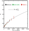 |
Fig. 4. N as a function of group area Agroup. The dashed line shows the best power-law fit to the data. |
3.3. Variation of R with solar activity
It is well known that many sunspot parameters, such as sunspot areas and number, exhibit periodic changes with the solar cycle (Hathaway 2015). Therefore, we also analyse the behaviour of R with time. In particular, we look for changes in R from cycle to cycle, as well as, during the activity maxima and minima. We first analyse the distribution of R during solar activity maxima and minima. For better statistics, we merged the data from all cycles and from all the observatories. We define cycle maxima and minima as 12 month periods centred at the times of the maxima and minima in the 13 month running mean of the sunspot area (in the merged series), respectively. There are significantly more bigger spots and groups during cycle maxima than during minima, while R depends on the group area (Fig. 3b). Hence, to eliminate this size dependency we first fit a lognormal function (R ∼ exp−[(log(Agroup)]2/2σ2]) to the data in Fig. 3b and then divide each measured R by the value this fit returns for the corresponding Agroup to obtain the normalised R value. Figure 5a shows these normalised R distributions for cycle maxima and minima in blue and red, respectively.
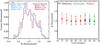 |
Fig. 5. Variation of R with solar activity. Panel a: distributions of R during sunspot maxima (in blue) and minima (in red) for the merged area data. Panel b: cycle-to-cycle variation of R (median) for the three individual observatories: Debrecen (black), Kislovodsk (green), and Pulkovo (red). The upper and lower limits of the error bars represent the third and first quartiles of corresponding R distributions. |
These distributions are nearly identical in shape and their mean, median, and mode values (listed in the legend) are very similar. We further test the hypothesis that the two samples come from the same distribution by applying the two-sided Kolmogorov–Smirnov (K–S) test which checks for the equivalence of two datasets by comparing their empirical cumulative distribution functions (ECDFs; Berger & Zhou 2014). The test statistics, D, is a measure of the difference between the ECDFs. The null hypothesis, that both samples come from the same underlying population, is rejected if D > Dcrit. On our two R distributions, D = 0.06 and Dcrit = 0.12, with a p value of 0.44. Thus, in our case the null hypothesis is true, and we conclude that no substantial variation in R is observed between the minimum and maximum of a sunspot cycle.
Finally, in Fig. 5b, we show the cycle-to-cycle variation of the normalised R. Filled circles represent the median values (second quartile) of R over each cycle, whereas the third and first quartiles of the corresponding R distributions are shown as the upper and lower limits of the error bars. We see no significant variation in R from cycle to cycle.
4. Conclusion
The analysis and understanding of the size distribution of sunspots and sunspot groups provides insights into the origin and evolution of solar magnetism. In this work we have investigated the distribution of the spot sizes within sunspot groups. Historical sunspot archives from the Kislovodsk (1954–2019), Pulkovo (1932–1991), and Debrecen (1974–2019) observatories have been analysed to derive the ratio, R, which is the area of the biggest spot in a group (Abig_spot) to the total area of that group (Agroup). Our conclusions are the following:
-
When considering all sunspot groups independently of their evolution the distribution of R shows a clear peak around 0.5 (i.e., a single big spot within a group occupies roughly 50% of the whole group area; see Fig. 2). The distribution, however, shows a secondary peak at or close to unity, which we attribute to the group’s evolution. Specifically, the following spots in a group typically emerge later and decay faster, so that during the initial and final stages of the group evolution the leading spot is often the only observable spot in the group or there are only small following spots.
-
By tracking individual groups over their lifetimes we find that at the time when the group area reaches its maximum, the biggest spot in a group typically occupies about 60% of the group area. For half of all groups, R lies in the range between roughly 50% and 70% (Fig. 3).
-
We also find that R changes with the group area, Agroup. In smaller groups (30 ≤ Agroup < 200 μHem), R increases from 0.55 to 0.65. It then decreases slightly before settling at a nearly constant value of about ≊0.6 for Agroup ≥ 700 μHem (Fig. 3).
-
The number of individual umbrae within a given group, N, increases with the group size as a power-law function of the form
 (Fig. 4). Since some spots have multiple umbrae, the number of individual spots within groups will increase less quickly with the group size than the rate given by this function.
 -
Extrapolation of our results to significantly bigger sunspot groups (such as unresolved starspot groups observed on highly active stars) suggests that such groups are composed of multiple spots, in agreement with the study by Solanki & Unruh (2004), and that a significant fraction (55–75%) of the group area is occupied by a single giant spot. We note, however, that these two conclusions are limited to spots formed by magnetic flux emerging in bipolar regions (e.g., Schuessler et al. 1996) and do not apply to starspots formed by magnetic flux being carried together, for example to the poles (Schrijver & Title 2001; Işık et al. 2018).
-
The distribution of R does not change between solar activity maxima and minima, and we see no cycle-to-cycle variation (Fig. 5).
In summary, this paper deals with the distribution of spots within a sunspot group, providing constraints on the flux emergence processes. In Babcock–Leighton dynamo models, flux emergence plays a key role as it is responsible for both toroidal magnetic flux through the photosphere (Cameron & Schüssler 2020) and for the generation of new poloidal magnetic flux through Joy’s law (Hale et al. 1919). Despite its critical role, the details of the emergence process remain poorly understood. For example, the cause of Joy’s law is not yet known; the Coriolis force is clearly implicated, but it is uncertain whether the underlying flows are those of the turbulent convective background (e.g., Parker 1955) or those internal to the rising flux tube (e.g., Caligari et al. 1995). We are now reaching the point where these possibilities can be modelled in detail. For example, there are numerical simulations starting from a magnetic flux concentration near the base of the convection zone and ending after the flux has emerged through the photosphere into the solar atmosphere (Hotta & Iijima 2020); there are also models where the magnetic and velocity fields from global dynamo simulations are coupled to models covering the emergence through the photosphere (Chen et al. 2017). Our findings of universal properties of this process, suggestive of a scale-invariant emergence pattern, are an observational constraint on the flux emergence process, which will be useful in evaluating the different model simulations, and is thus critical for understanding the solar dynamo. Our findings require, in order to match the observations, that the ratio of the area of the largest spot in a group to the area of all spots in the group should be approximately 0.55–0.65 for the vast majority of sunspot groups. More conservatively, we can say that a very strong constraint emerging from our work is that the largest sunspot covers more than half the area of the whole sunspot group, and hence also carries more than half of the magnetic flux. Flux emergence is also a critical driver of the dynamics of the solar atmosphere, and our results are also relevant for understanding and modelling the atmospheric response to flux emergence where the distribution of the field at the surface is important. Further studies using a combination of simultaneous white-light and magnetic data, for example from SoHO/MDI (Scherrer et al. 1995), SDO/HMI (Lemen et al. 2012), or in the future from SO/PHI (Solanki et al. 2020), will additionally help us to understand the relation between the magnetic flux distribution and the observed spot distribution within a group.
Further details are available at http://fenyi.solarobs.csfk.mta.hu/ftp/pub/DPD/DPDformat.txt
Acknowledgments
We thank the anonymous reviewer for the encouraging comments and helpful suggestions. We also thank the teams of the archives used in this study for all the work they had invested into obtaining and making these data available to the community.
References
- Balmaceda, L. A., Solanki, S. K., Krivova, N. A., & Foster, S. 2009, J. Geophys. Res. A: Space Phys., 114, A07104 [Google Scholar]
- Balthasar, H., Vazquez, M., & Woehl, H. 1986, A&A, 155, 87 [Google Scholar]
- Baranyi, T., Gyori, L., Ludmány, A., & Coffey, H. E. 2001, MNRAS, 323, 223 [Google Scholar]
- Baranyi, T., Király, S., & Coffey, H. E. 2013, MNRAS, 434, 1713 [Google Scholar]
- Baranyi, T., Győri, L., & Ludmány, A. 2016, Sol. Phys., 291, 3081 [Google Scholar]
- Baumann, I., & Solanki, S. K. 2005, A&A, 443, 1061 [NASA ADS] [CrossRef] [EDP Sciences] [Google Scholar]
- Berdyugina, S. V. 2005, Liv. Rev. Sol. Phys., 2, 8 [Google Scholar]
- Berger, V. W., & Zhou, Y. 2014, Kolmogorov–Smirnov Test: Overview (American Cancer Society) [Google Scholar]
- Bogdan, T. J., Gilman, P. A., Lerche, I., & Howard, R. 1988, ApJ, 327, 451 [Google Scholar]
- Borrero, J. M., & Ichimoto, K. 2011, Liv. Rev. Sol. Phys., 8, 4 [Google Scholar]
- Bray, R. J., & Loughhead, R. E. 1979, Sunspots [Google Scholar]
- Bumba, V. 1963, Bull. Astron. Inst. Czech., 14, 91 [Google Scholar]
- Caligari, P., Moreno-Insertis, F., & Schussler, M. 1995, ApJ, 441, 886 [Google Scholar]
- Cameron, R. H., & Schüssler, M. 2020, A&A, 636, A7 [CrossRef] [EDP Sciences] [Google Scholar]
- Chen, F., Rempel, M., & Fan, Y. 2017, ApJ, 846, 149 [NASA ADS] [CrossRef] [Google Scholar]
- Fligge, M., & Solanki, S. K. 1997, Sol. Phys., 173, 427 [Google Scholar]
- Győri, L., Ludmány, A., & Baranyi, T. 2017, MNRAS, 465, 1259 [Google Scholar]
- Hale, G. E., Ellerman, F., Nicholson, S. B., & Joy, A. H. 1919, ApJ, 49, 153 [NASA ADS] [CrossRef] [Google Scholar]
- Hathaway, D. H. 2015, Liv. Rev. Sol. Phys., 12, 4 [Google Scholar]
- Hathaway, D. H., & Choudhary, D. P. 2008, Sol. Phys., 250, 269 [Google Scholar]
- Hotta, H., & Iijima, H. 2020, MNRAS, 494, 2523 [Google Scholar]
- Howard, R. F. 1992, Sol. Phys., 137, 51 [Google Scholar]
- Işık, E., Solanki, S. K., Krivova, N. A., & Shapiro, A. I. 2018, A&A, 620, A177 [NASA ADS] [CrossRef] [EDP Sciences] [Google Scholar]
- Karak, B. B., & Brandenburg, A. 2016, ApJ, 816, 28 [Google Scholar]
- Kolmogorov, A. 1941, Akademiia Nauk SSSR Doklady, 30, 301 [Google Scholar]
- Kuklin, G. V. 1980, Bull. Astron. Inst. Czech., 31, 224 [Google Scholar]
- Lemen, J. R., Title, A. M., Akin, D. J., et al. 2012, Sol. Phys., 275, 17 [Google Scholar]
- Mandal, S., & Banerjee, D. 2016, ApJ, 830, L33 [Google Scholar]
- Mandal, S., Krivova, N. A., Solanki, S. K., Sinha, N., & Banerjee, D. 2020, A&A, 640, A78 [CrossRef] [EDP Sciences] [Google Scholar]
- McIntosh, P. S. 1981, in The Physics of Sunspots, eds. L. E. Cram, & J. H. Thomas, 7–54 [Google Scholar]
- Mikhailov, A. 1955, The Observatory, 75, 28 [Google Scholar]
- Muñoz-Jaramillo, A., Senkpeil, R. R., Windmueller, J. C., et al. 2015, ApJ, 800, 48 [Google Scholar]
- Muraközy, J. 2020, ApJ, 892, 107 [Google Scholar]
- Muraközy, J. 2021, ApJ, 908, 133 [Google Scholar]
- Muraközy, J., Baranyi, T., & Ludmány, A. 2014, Sol. Phys., 289, 563 [Google Scholar]
- Nagovitsyn, Y. A., & Pevtsov, A. A. 2016, ApJ, 833, 94 [Google Scholar]
- Nagovitsyn, Y. A., Makarova, V. V., & Nagovitsyna, E. Y. 2007, Sol. Syst. Res., 41, 81 [Google Scholar]
- Nagovitsyn, Y. A., Pevtsov, A. A., & Livingston, W. C. 2012, ApJ, 758, L20 [Google Scholar]
- Parker, E. N. 1955, ApJ, 121, 491 [Google Scholar]
- Parnell, C. E., DeForest, C. E., Hagenaar, H. J., et al. 2009, ApJ, 698, 75 [Google Scholar]
- Pietarila Graham, J., Cameron, R., & Schüssler, M. 2010, ApJ, 714, 1606 [Google Scholar]
- Rempel, M. 2014, ApJ, 789, 132 [Google Scholar]
- Rempel, M., & Cheung, M. C. M. 2014, ApJ, 785, 90 [Google Scholar]
- Ross, S. M. 2000, Introduction to Probability and Statistics for Engineers and Scientists [Google Scholar]
- Scherrer, P. H., Bogart, R. S., Bush, R. I., et al. 1995, Sol. Phys., 162, 129 [Google Scholar]
- Schrijver, C. J., & Title, A. M. 2001, ApJ, 551, 1099 [Google Scholar]
- Schrijver, C. J., Title, A. M., van Ballegooijen, A. A., Hagenaar, H. J., & Shine, R. A. 1997, ApJ, 487, 424 [NASA ADS] [CrossRef] [Google Scholar]
- Schuessler, M., Caligari, P., Ferriz-Mas, A., Solanki, S. K., & Stix, M. 1996, A&A, 314, 503 [Google Scholar]
- Solanki, S. K. 2003, A&ARv, 11, 153 [Google Scholar]
- Solanki, S. K., & Unruh, Y. C. 2004, MNRAS, 348, 307 [Google Scholar]
- Solanki, S. K., del Toro Iniesta, J. C., Woch, J., et al. 2020, A&A, 642, A11 [CrossRef] [EDP Sciences] [Google Scholar]
- Stenflo, J. O. 2012, A&A, 547, A93 [NASA ADS] [CrossRef] [EDP Sciences] [Google Scholar]
- Strassmeier, K. G. 2009, A&ARv, 17, 251 [NASA ADS] [CrossRef] [Google Scholar]
- Thornton, L. M., & Parnell, C. E. 2011, Sol. Phys., 269, 13 [Google Scholar]
- Tlatov, A. G., & Pevtsov, A. A. 2014, Sol. Phys., 289, 1143 [Google Scholar]
- van Driel-Gesztelyi, L., & Green, L. M. 2015, Liv. Rev. Sol. Phys., 12, 1 [NASA ADS] [CrossRef] [Google Scholar]
All Tables
All Figures
|
Fig. 1. Images of two sunspot groups (NOAA 7790 and NOAA 7680) from Debrecen observatory (These images are available at http://fenyi.solarobs.csfk.mta.hu/en/databases/DPD/). In each image individual umbrae are labelled with unique numbers. |
| In the text | |
|
Fig. 2. Results from the instantaneous distribution analysis. Panel a: normalised distribution of R from Debrecen (black), Kislovodsk (green), and Pulkovo (red) when considering all daily individual groups, i.e., irrespective of their evolutionary phase. Panel b: same as panel a, but after removing groups with N = 1 and Agroup ≤ 30 μHem. |
| In the text | |
|
Fig. 3. Results from the tracked data. Panel a: normalised distribution of R calculated at the time of maximum Agroup. Panel b: R as a function of Agroup. The error bars represent the standard deviations calculated for each bin. Panel c: same as panel b, but averaged over the three individual datasets. The dashed line is the linear fit to the data between 500 and 1200 μHem, whereas the grey shading highlights the 1σ uncertainty of the fit. |
| In the text | |
|
Fig. 4. N as a function of group area Agroup. The dashed line shows the best power-law fit to the data. |
| In the text | |
|
Fig. 5. Variation of R with solar activity. Panel a: distributions of R during sunspot maxima (in blue) and minima (in red) for the merged area data. Panel b: cycle-to-cycle variation of R (median) for the three individual observatories: Debrecen (black), Kislovodsk (green), and Pulkovo (red). The upper and lower limits of the error bars represent the third and first quartiles of corresponding R distributions. |
| In the text | |
Current usage metrics show cumulative count of Article Views (full-text article views including HTML views, PDF and ePub downloads, according to the available data) and Abstracts Views on Vision4Press platform.
Data correspond to usage on the plateform after 2015. The current usage metrics is available 48-96 hours after online publication and is updated daily on week days.
Initial download of the metrics may take a while.