| Issue |
A&A
Volume 681, January 2024
|
|
|---|---|---|
| Article Number | A65 | |
| Number of page(s) | 20 | |
| Section | Stellar structure and evolution | |
| DOI | https://doi.org/10.1051/0004-6361/202347195 | |
| Published online | 16 January 2024 | |
Cepheid Metallicity in the Leavitt Law (C- MetaLL) survey
IV. The metallicity dependence of Cepheid period–luminosity relations⋆
1
Leibniz-Institut für Astrophysik Potsdam (AIP), An der Sternwarte 16, 14482 Potsdam, Germany
e-mail: This email address is being protected from spambots. You need JavaScript enabled to view it.
2
Institut für Physik und Astronomie, Universität Potsdam, Haus 28, Karl-Liebknecht-Str. 24/25, 14476 Golm, Potsdam, Germany
3
INAF-Osservatorio Astronomico di Capodimonte, Salita Moiariello 16, 80131 Naples, Italy
4
INAF-Osservatorio Astrofisico di Catania, Via S. Sofia 78, 95123 Catania, Italy
5
Istituto Nazionale di Fisica Nucleare (INFN)-Sez. di Napoli, Via Cinthia, 80126 Napoli, Italy
6
INAF – Osservatorio Astronomico di Roma, Via Frascati 33, 00078 Monte Porzio Catone, Italy
7
INAF-Osservatorio di Astrofisica e Scienza dello Spazio, Via Gobetti 93/3, 40129 Bologna, Italy
Received:
15
June
2023
Accepted:
5
October
2023
Abstract
Context. Classical Cepheids (DCEPs) play a fundamental role in the calibration of the extragalactic distance ladder, which eventually leads to the determination of the Hubble constant (H0) thanks to the period–luminosity (PL) and period–Wesenheit (PW) relations exhibited by these pulsating variables. Therefore, it is of great importance to establish the dependence of PL and PW relations on metallicity.
Aims. We aim to quantify the metallicity dependence of the PL and PW relations of the Galactic DCEPs for a variety of photometric bands, ranging from optical to near-infrared.
Methods. We gathered a literature sample of 910 DCEPs with available [Fe/H] values from high-resolution spectroscopy or metallicities from the Gaia Radial Velocity Spectrometer. For all these stars, we collected photometry in the GBP, GRP, G, I, V, J, H, and KS bands and astrometry from Gaia Data Release 3 (DR3). We used these data to investigate the metal dependence of both the intercepts and slopes of a variety of PL and PW relations at multiple wavelengths.
Results. We find a large negative metallicity effect on the intercept (γ coefficient) of all the PL and PW relations investigated in this work, while present data still do not allow us to draw firm conclusions regarding the metal dependence of the slope (δ coefficient). The typical values of γ are around −0.4 : −0.5 mag dex−1, which is larger than most of the recent determinations present in the literature. We carried out several tests, which confirm the robustness of our results. As in our previous works, we find that the inclusion of a global zero point offset of Gaia parallaxes provides smaller values of γ (in an absolute sense). However, the assumption of the geometric distance of the Large Magellanic Cloud seems to indicate that larger values of γ (in an absolute sense) would be preferred.
Key words: stars: variables: Cepheids / stars: distances / distance scale / stars: abundances / stars: fundamental parameters
Full Table 1 is available at the CDS via anonymous ftp to cdsarc.cds.unistra.fr (130.79.128.5) or via https://cdsarc.cds.unistra.fr/viz-bin/cat/J/A+A/681/A65
© The Authors 2024
 Open Access article, published by EDP Sciences, under the terms of the Creative Commons Attribution License (https://creativecommons.org/licenses/by/4.0), which permits unrestricted use, distribution, and reproduction in any medium, provided the original work is properly cited.
This article is published in open access under the Subscribe to Open model. This email address is being protected from spambots. You need JavaScript enabled to view it. to support open access publication.
1. Introduction
Classical Cepheids (DCEPs) are the most important standard candles of the extragalactic distance scale thanks to the Leavitt Law (Leavitt & Pickering 1912), which is a relationship between period and luminosity (PL) of DCEPs. Once calibrated using independent distances based on geometric methods such as trigonometric parallaxes, eclipsing binaries, and water masers, these relations constitute the first step in forming the cosmic distance scale, as they calibrate secondary distance indicators. These latter include Type Ia supernovae (SNIa), which in turn allow us to measure the distances of distant galaxies located in the steady Hubble flow. The calibration of this three-step procedure (also called the cosmic distance ladder) allows us to reach the Hubble flow, where the constant (the Hubble constant H0) that connects the distance to the recession velocity of galaxies can be estimated (e.g., Sandage & Tammann 2006; Freedman et al. 2012; Riess et al. 2016, and references therein). The value of H0 is an important quantity in cosmology because it sets the dimension and the age of the Universe. Therefore, measuring the value of the constant with an accuracy of 1% is one of the most important quests of modern astrophysics. However, there is currently a well-known discrepancy between the values of H0 obtained by the SH0ES1 project through the cosmic distance ladder (H0 = 73.01 ± 0.99 km s−1 Mpc−1, Riess et al. 2022) and those measured by the Planck Cosmic Microwave Background (CMB) project using the flat Λ cold dark matter (ΛCDM) model (H0 = 67.4 ± 0.5 km s−1 Mpc−1, Planck Collaboration VI 2020). No solution has yet been proposed for this 5σ discrepancy, and if confirmed, it would highlight the need for a revision of the ΛCDM model.
In this context, one of the residual sources of uncertainty in the cosmic distance ladder is represented by the debated metallicity dependence of the DCEP PL relations used to calibrate the secondary distance indicators. Indeed, a metallicity variation is predicted to affect the shape and width of the DCEP instability strip (e.g., Caputo et al. 2000), which in turn affects the coefficient of the PL relations (Marconi et al. 2005, 2010; De Somma et al. 2022, and references therein). The dependence of the PL relations and of the reddening-free Wesenheit magnitudes2 on metallicity, however small, when involving near-infrared (NIR, see e.g., Fiorentino et al. 2013; Gieren et al. 2018) colours must be taken into account to avoid systematic effects in the calibration of the extragalactic distance scale (e.g., Romaniello et al. 2008; Bono et al. 2010; Riess et al. 2016).
Direct empirical evaluations of the metallicity dependence of PL relations using Galactic DCEPs with sound [Fe/H] measurements based on high-resolution (HiRes hereafter) spectroscopy have been hampered so far by the lack of accurate independent distances for a significant number of Milky Way (MW) DCEPs. The advent of the Gaia mission (Gaia Collaboration 2016) has completely changed this scenario. Gaia began providing accurate parallaxes with data release 2 (DR2 Gaia Collaboration 2018), which were further improved with the early data release 3 (Gaia Collaboration 2021). In addition, the Gaia mission secured the discovery of hundreds of new Galactic DCEPs (Clementini et al. 2019; Ripepi et al. 2019, 2022) which, together with those discovered by other surveys, such as the OGLE Galactic Disk survey (Udalski et al. 2018) and the Zwicky Transient Facility (ZTF Chen et al. 2020), constitute a formidable sample of DCEPs useful not only in the context of the extragalactic distance scale but also for Galactic studies (e.g., Lemasle et al. 2022; Trentin et al. 2023, and references therein). However, until a few years ago, the number of DCEPs with metallicity measurements from HiRes spectroscopy was mainly restricted to the solar neighbourhood, where the DCEPs span a limited range in [Fe/H], centred on solar or slightly supersolar values, with a small dispersion of 0.2–0.3 dex (e.g., Genovali et al. 2014; Luck 2018; Groenewegen 2018; Ripepi et al. 2019). This makes it very difficult to measure the metallicity dependence of PL relations using Galactic Cepheids with sound statistical significance.
In this context, a few years ago we started a project named C-MetaLL (Cepheid - Metallicity in the Leavitt Law, see Ripepi et al. 2021a, for a full description), with the goal being to measure the chemical abundance of a sample of 250–300 Galactic DCEPs through HiRes spectroscopy, expressly aiming to enlarge the iron abundance range towards the metal-poor regime – that is, [Fe/H] < −0.4 dex – where only a few stars have abundance measurements in the literature. In the first two papers of the series (Ripepi et al. 2021a; Trentin et al. 2023), we published accurate abundances for more than 25 chemical species for a total of 114 DCEPs. In particular, in Trentin et al. (2023), we obtained measures for 43 objects with [Fe/H] < −0.4 dex, reaching abundances of as low as −1.1 dex. The scope of this paper is to study the metallicity dependence of the PL relations using a [Fe/H] range of more than 1 dex. In this way, we aim to be able to discern between the two scenarios that came out in the recent literature concerning the metallicity dependence of PL relations. In fact, in our previous works using Galactic DCEPs and Gaia parallaxes, we found a rather large dependence in the NIR bands of on the order of ∼ − 0.4 mag dex−1 (Ripepi et al. 2020, 2021a); or even larger when using the Gaia bands (∼ − 0.5 mag dex−1Ripepi et al. 2022). These values are discrepant with those measured by the SH0ES group (∼ − 0.2 mag dex−1Riess et al. 2021) – which, on the other hand, used a calibrating sample of 75 DCEPs in the solar vicinity spanning a small [Fe/H] range–, and are also different from those measured by Breuval et al. (2021, 2022), who obtained similar results to the SH0ES group using three Cepheid samples in the Milky Way and the Large and Small Magellanic Clouds (LMC and SMC, respectively) as three representative objects with different mean metallicities.
The paper is organized as follows: in Sect. 2 we describe the sample of DCEPs and their properties. In Sect. 3, we describe the method we used to derive the period–luminosity–metallicity (PLZ) and period–Wesenheit–metallicity (PWZ) relations; in Sects. 4 and 5, we describe and discuss our results; and in Sect. 6 we outline our conclusions.
2. Description of the data used in this work
In this section, we describe the sample of DCEPs used in this paper and their photometric, spectroscopic, and astrometric properties. All the data employed in our analysis are listed in Table 1.
Photometric, astrometric, and spectroscopic data for the DCEP sample used in this work.
2.1. Photometry
Optical V, I3 photometry is available in the literature for about 488 and 364 DCEPs of our sample, respectively (Groenewegen 2018; Ripepi et al. 2021a). For the remaining stars, we decided to use the homogeneous and precise Gaia G, GBP, GRP photometry transformed into the Johnson-Cousins V, I bands by means of the relations published by Pancino et al. (2022). We calculated these aforementioned magnitudes for all the stars with full G, GBP, GRP values (all DCEPs except one) using the intensity-averaged magnitudes from the Gaia Vizier catalogue I/358/vcep (Ripepi et al. 2022) or the simple average magnitudes from the Gaia source catalogue (Vizier I/355/gaiadr3) for the few stars not present in the quoted catalogue. Figure 1 shows the comparison between the literature V, I magnitudes and those calculated from the Gaia photometry for the stars for which both values are available. While the transformed V photometry appears perfectly compatible with that from the literature (VLit − VGaia ∼ 0.0 with dispersion σ ∼ 0.04 mag), the transformed I photometry appears to be slightly too faint: ILit − IGaia ∼ 0.035 (mag) with a dispersion of σ ∼ 0.035 mag. Therefore, we used the transformed V bands with no modification, while we corrected the transformed I bands by increasing their value by 0.035 mag. As for the uncertainties, we assumed 0.02 mag in both V and I for the literature sample when the number is not available in the original publication, while for the remaining stars, we propagated the errors, also taking into account (summing in quadrature) the uncertainties in the transformations provided by Pancino et al. (2022). For a handful of stars, the DCEPs (GBP − GRP) colours were beyond the validity limit of the Pancino et al. (2022) relations. For these stars, we adopted the synthetic V, I magnitudes calculated by Montegriffo (2023) based on Gaia DR3 photometry.
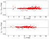 |
Fig. 1. Comparison between the literature V, I photometry and that from Gaia through the transformation by Pancino et al. (2022). The top and bottom panels show the comparison in V and I bands, respectively. |
Near-infrared J, H, and KS band photometry is from van Leeuwen et al. (2007), Gaia Collaboration (2017), Groenewegen (2018) and Ripepi et al. (2021a) for the literature sample, and is derived from single-epoch 2MASS photometry (Skrutskie et al. 2006) for the remaining stars. To this aim, we adopted the procedure outlined in Ripepi et al. (2021a), using the ephemerides (periods and epochs of maximum light) from the Gaia Vizier catalogue I/358/vcep. As in our previous work, the uncertainties on the mean magnitudes were calculated using Monte Carlo simulations, varying the 2MASS magnitude and the phase of the single-epoch photometry within their errors, where the last quantity was calculated using the errors on the periods given in the Gaia catalogue.
In this work, we also considered the Wesenheit indices, which are reddening-free quantities by construction (Brodie & Madore 1980). These are obtained by combining the standard magnitude in a given photometric band with a colour term according to the following equation:
 (1)
(1)
where Xi indicates the generic band and the coefficient  coincides with the total-to-selective absorption and is obtained by assuming an extinction law. The photometric band combinations adopted in this work are listed in Table 2, together with the coefficient of the colour term. In order to transform the Johnson-Cousins-2MASS ground-based H, V, and I photometry into the HST correspondent F160W, F555W, and F814W filters, we considered the photometric transformations by Riess et al. (2021). We note that, for brevity, in the following the calibrated Wesenheit in the HST bands is referred to as
  4.
4.
Photometric bands and colour coefficients adopted to calculate the Wesenheit magnitudes considered in this work.
In analogy with photometry, the reddening for the literature sample was taken from van Leeuwen et al. (2007), Gaia Collaboration (2017), Groenewegen (2018) and Ripepi et al. (2021a), while for the remaining stars, we used the same period–colour relations used in Ripepi et al. (2021a) involving (V − I) colour (their Eq. (4)), obtaining E(V − I) excesses that were converted into the corresponding E(B − V) ones using the relation E(V − I) = 1.28 E(B − V) (Tammann et al. 2003). The uncertainties on these reddening values were calculated by summing in quadrature the rms of Eq. (4) in Ripepi et al. (2021a), with the errors on V and I magnitudes. However, to be conservative, we assumed an uncertainty of 10% on the reddening for values of E(B − V) > 1.0 mag.
2.2. Metallicity
Metallicities were taken from various literature sources. A large part of the sample is the same as in Trentin et al. (2023, see their Sect. 4.1). More specifically, we considered the large compilation of homogenised literature iron abundances for 436 DCEPs presented by Groenewegen (2018, G18 hereinafter), complemented with literature results for a few additional stars by Gaia Collaboration (2017, GC17 hereinafter). To these data, we added the following samples: (i) 49 DCEPs presented in Catanzaro et al. (2020), Ripepi et al. (2021a,b collectively called R21 hereinafter); (ii) the sample of 65 DCEPs published in Trentin et al. (2023, called T23 hereafter); (iii) the 104 stars by Kovtyukh et al. (2022, K22 hereinafter) after removing the large overlap with the R21 and T23 sample (see Trentin et al. 2023, for full details and the homogenisation procedure we adopted in merging the samples); and (iv) a few stars with HiRes metallicities from the GALAH Survey (GALactic Archaeology with HERMES; Buder et al. 2021, stars OGLE-GD-CEP-0059, OGLE-GD-CEP-0058, V1253 Cen) and from the PASTEL catalogue (Soubiran et al. 2016, star OGLE-GD-CEP-0117). With these additions, the total number of DCEPs with metallicities from HiRes spectroscopy is 635. Concerning homogeneity, apart from the few stars from GALAH, PASTEL, or GC17, the main samples adopted in this work are the G18, K22, and combined C-MetaLL data. As mentioned above, the G18 sample is already homogeneous, while the K22 abundances were homogenised with those of the C-MetaLL sample in Trentin et al. (2023). As discussed in Ripepi et al. (2021b), the C-MetaLL data have only two stars in common with G18, namely X Sct and V5567 Sgr. For these two stars, the abundances agree well within 0.5σ.
In addition to this already large sample, we decided to exploit the recent results released by the Gaia DR3. To this aim, we cross-matched the DCEP catalogue published by Gaia DR3 (Vizier catalogue I/358/vcep) as amended by Ripepi et al. (2022) with that of the astrophysical parameters (Vizier catalogue I/355/paramp), retaining only matching stars that have a global metallicity value ([M/H]) derived from the medium-resolution spectra obtained with the Radial Velocity Spectrometer (RVS, see Recio-Blanco et al. 2023, for details). The total number of matching stars is 983, among which 475 have HiRes metallicity estimations from the literature. Gaia metallicities were corrected following the recipe by Recio-Blanco et al. (2023, their Eq. (4) and Table 5), and then we assigned a data-quality flag to every object. Assigned flags are 1, 2, and 3, which refer to high-, medium-, and low-quality, respectively, according to Recio-Blanco et al. (2023, see Sect. 9). The Gaia abundances were derived using the stacked RVS spectra over all the epochs of observations. The resulting spectra are therefore an average of many spectra over the pulsation cycle. As the DCEPs vary in terms of effective temperature, surface gravity, and microturbulent velocity along the pulsation cycle, we can in principle expect an impact on the derived abundances. In addition, the abundances published in the Gaia Astrophysical parameters are the mean metallicities [M/H], which may differ from the [Fe/H] scale used for the HiRes sample. To investigate these potential concerns, we compared the corrected Gaia metallicities with those from the HiRes sample for the 475 stars in common. The result is shown in Fig. 2. There is good overall agreement for all the Gaia subsamples (low, medium, and high quality). In all cases, the average difference between HiRes and Gaia results is very low, namely Δ ∼ −0.03 dex, with a comfortable moderate dispersion of the order of 0.11–0.13 dex (worse for the low-quality Gaia data), indicating that the Gaia spectroscopic results are of comparable quality to the HiRes ones overall and that the data can be used together. This is especially true for [Fe/H]HiRes > −0.3 dex. Below this value, the Gaia sample is dominated by low-quality data and the dispersion becomes significantly larger (top panel). We corrected for the small offset of the Gaia data and decided to use only the medium- and high-quality data in the following in order to avoid including some unreliable abundance values from the low-quality data. The resulting sample is then composed of 910 DCEPs divided into 282 DCEP_1Os, 22 DCEP_1O2Os, 581 DCEP_Fs, and 25 DCEP_F1Os, where DCEP_1O2Os and DCEP_F1Os represent multi-mode pulsators. For these two last cases, we adopted the longest period, that is, the 1O period for the 1O2O pulsators and the F one for the F1O DCEPs. Therefore, our sample includes the equivalent of 304 1O and 606 F mode DCEPs.
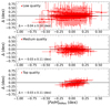 |
Fig. 2. Comparison between the [Fe/H] from HiRes data and Gaia [M/H]. From top to bottom, the different panels show the comparison for the low-, medium-, and high-quality Gaia data, respectively (see text for details). In each panel, the average difference Δ and its dispersion is displayed. |
2.3. Astrometry
To carry out our analysis, we adopted the parallaxes from Gaia DR3, which were individually corrected for the zero point offset, adopting the recipe by Lindegren et al. (2021, L21)5. We highlight the characteristic shape of the correction, with a sharp hump around G ∼ 12 mag, the explanation for which can be found in Lindegren et al. (2021). The individual corrections are shown in Fig. 3 as a function of the magnitude and of the ecliptic latitude. As criteria of the goodness of the astrometry, we adopted two indicators: (i) the fidelity_v2 index as tabulated by Rybizki et al. (2022), retaining only objects with values larger than 0.5, and (ii) the RUWE parameter published in Gaia DR3. Although the Gaia documentation recommends using a threshold below 1.4 for good astrometric solutions, we choose to be less conservative and use a slightly larger threshold equal to 1.5. This choice allows us to retain possibly good objects falling just outside the 1.4 threshold. In any case, our robust outlier-removal procedure (see Sect. 3) removes possible deviating stars introduced by the slightly enlarged adopted threshold.
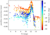 |
Fig. 3. Individual parallax corrections from L21 as a function of the G magnitude. The points are colour coded according to the ecliptic latitude. |
The simultaneous use of the fidelity_v2 and RUWE parameters led us to reject 78 objects from our sample. A large fraction of the rejected DCEPs, namely 35, have G ≤ 7 mag. This is not surprising, as Gaia parallaxes are known to be uncertain for such bright stars (e.g., Lindegren et al. 2021).
3. Derivation of the PLZ/PWZ relations
In this section, we describe the procedure adopted to calibrate the PLZ/PWZ relations. The approach is the same as in Ripepi et al. (2020); Ripepi et al. (2021a). To avoid any bias, the whole DCEPs sample was considered, including negative parallaxes, and without any selection on the parallax relative errors. Moreover, we adopted the astrometry-based-luminosity (ABL) formalism (Feast & Catchpole 1997; Arenou & Luri 1999), which allows us to treat the parallax ϖ as a linear parameter:
![Mathematical equation: $$ \begin{aligned} \mathrm{ABL}=\varpi 10^{0.2 m -2}=10^{0.2(\alpha +(\beta +\delta \mathrm{[Fe/H])}(\log P-\log P_0) +\gamma \mathrm{[Fe/H]})}, \end{aligned} $$](/articles/aa/full_html/2024/01/aa47195-23/aa47195-23-eq5.gif) (2)
(2)
where the parallax ϖ, the apparent generic magnitude m, the period P, and the metallicity [Fe/H] are the observables, while the unknowns are the four parameters α, β, γ, and δ (intercept, slope, metallicity dependence of the intercept, and the metallicity dependence of the slope, respectively). The P0 quantity is a pivoting period (10 d) adopted to reduce the correlation between the α and β parameters, which dominate the PL and PW relations.
To take into account the presence of possible outlier measurements, we applied multiple sigma-clipping removals but limited the number of rejected data to ∼10% of the full sample. Based on the results described in the previous papers of this series, we decided to exclude the case with no metallicity dependence at all (i.e., γ ≠ 0) in Eq. (2). Finally, the 1O pulsators are included in the fitting sample by fundamentalising their periods according to the relation by Alcock et al. (1995) and Feast & Catchpole (1997). In the following sections, we consider two data samples: (i) the Lit+DR3 sample, which includes all the selected sources introduced in Sect. 2; and (ii) the Lit sample, which was obtained by excluding the sources with only a Gaia DR3 metallicity estimate, therefore retaining only DCEPs with metallicity measures from ground-based HiRes spectrographs.
The uncertainties on the parameters calculated in the following analysis are obtained through the bootstrap technique. A set of 1000 resampling experiments is performed and the coefficients of the Eq. (2) are calculated for each obtained random data set. Finally, the quoted errors are estimated by considering the robust standard deviation of the obtained coefficient distributions.
4. Results
4.1. Literature and Gaia DR3 sample
The results of the fitting procedure obtained for this case are listed in Table 3. We studied the dependence of the fitted PLZ/PWZ coefficients on the central wavelength of the considered filters. To associate a characteristic wavelength to the Wesenheit magnitudes, we decided to consider the central wavelength of the main band (e.g., G band for the WG, BP − RP case). The results of this analysis are shown in Fig. 4 for the F+1O sample (i.e., the sample including both F and fundamentalised 1O pulsators) and assuming a metallicity dependence also in the slope of the PLZ/PWZ relation (i.e., δ ≠ 0). Looking at the PLZ coefficients (blue filled circles), a strong linear dependence as a function of the λ−1 is evident only for the α and β coefficients (correlation coefficient R2 ≃ 1), while for γ and δ the slope of the fit is consistent with zero. The relations between α, β, and λ−1 are the following:

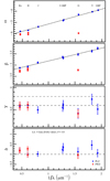 |
Fig. 4. Coefficients of PLZ/PWZ relations obtained from the fit to the Lit.+Gaia sample plotted against the λ−1 parameter. From top to bottom, the panels correspond to the α, β, γ, and δ coefficients. In each panel, PLZ and PWZ coefficients are plotted with blue and red symbols respectively, while the solid line shows the linear fit only for the PLZ relations. Grey dashed lines in the γ panel delimit the range of results in the literature (−0.2 to −0.4 mag dex−1, see Breuval et al. 2022, and Sect. 5.4), while in the δ panel, it corresponds to the value 0. |
Results of the fitting using the Lit.+ Gaia data set.
with rms = 0.019, R2 = 0.99, and

with rms = 0.059, R2 = 0.99. The strong dependence of the slope on the wavelength is a well-known feature, as thoroughly discussed by Madore & Freedman (2011).
A similar discussion is valid for the case where the δ coefficient is neglected in Eq. (2). The estimated parameters are shown in Fig. 5, while the linear equations for α and β coefficients are the following:

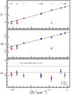 |
Fig. 5. Same as Fig. 4 but for the case neglecting the metallicity dependence in the PLZ/PLW slope (i.e., δ = 0). |
with rms = 0.02, R2 = 0.99, and

with rms = 0.06, R2 = 0.99.
Comparing these results with those in the previous case, we found good agreement between all the parameters. To easily compare our γ values with those in the recent literature, we traced two reference lines in the third panel of Figs. 4 and 5 corresponding to γ = −0.2 and −0.4 dex. Indeed, this range of values includes almost all the recent estimates for the value of γ (see Table 1 of Breuval et al. 2022, and Sect. 5.4 for a comprehensive list of recent results). Concerning the δ parameter, the bottom panel of Fig. 4 shows a significant metallicity dependence of the slopes only in the cases of the V-band PL. We note that in this case, the corresponding γ coefficients is highly consistent with the average literature values.
For the sake of completeness, in Appendix A we also plot the results obtained by fitting the Eq. (2) to the sample including only the F pulsators (see Figs. A.1 and A.2). The exclusion of the fundamentalised 1O pulsators increases the errors on all the coefficients, especially for δ. More specifically, we notice that the α and the β coefficients, within the errors, are found to be slightly increased and decreased, respectively, while the γ values are bigger (in an absolute sense), except for cases of the G and Gbp magnitudes. The δ parameter assumes also higher values in general and is more scattered compared with the F+1O case, but the large uncertainties prevent us from drawing firm conclusions.
To help in visualisation of the fitted relations listed in Table 3, we considered δ = 0, because in this case, the dependence on log(P) in Eq. (2) can be separated from that on metallicity. Figures 6 and 7 show the projections of the PLZ relations in two dimensions using P and [Fe/H] on the x-axis, respectively. Similarly, Figs. 8 and 9 display the same projections for the PWZ relations. Figures 6 and 8 show no colour trend with metallicity, indicating that the correction for this parameter was effective. On the other hand, Figs. 7 and 9 display the metallicity dependence of the intercepts of the PL and PW relations, respectively, in a direct way. In these figures, the slopes of the solid lines, representing the fits for the different magnitudes, are a direct visualisation of the values of γ. It is possible to appreciate the relevance and importance of the extension towards the metal-poor regime for the determination of this parameter. Indeed, even a small number of objects with [Fe/H] < −0.4 dex can significantly affect and constrain the slope in these plots.
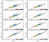 |
Fig. 6. PL relations for the bands studied in the paper where the magnitudes have been subtracted by the metallicity contribution. The colour bar represents the metallicity. |
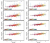 |
Fig. 7. Visualization of the PL dependence on the metallicity. The y-axis is the magnitudes subtracted by the period contribution and the x-axis is the metallicity. The colour bar represents the logarithm of the period. |
4.2. Literature sample only
The results of the fitting procedure obtained including the literature sample only are listed in Table 4. Similarly to the case above, we fitted α and β coefficients as a function of λ−1 of the specific band (only for PLZ). These fits are shown in the top two panels of Fig. 10 and their equations are:

Fitting results from the Lit. data set.
with rms = 0.04, R2 = 0.99, and

with rms = 0.06, R2 = 0.99. The fits shown in Fig. 5 (δ = 0 case for the Lit. sample) for α and β are respectively

with rms = 0.035, R2 = 0.99, and

with rms = 0.057, R2 = 0.99.
The inclusion of the δ parameter in the fit of the Lit. sample only determines a general decrease (in an absolute sense) in the γ values, which are closer to the −0.2,−0.4 mag dex−1 range typical of previous works. However, at the same time, the δ parameters show a considerable dependence of the PLZ/PWZ slopes on metallicity. If instead the δ parameter is neglected, as shown in Fig. 11, we again find an increase in the absolute value of γ, as already found for the Lit.+Gaia case. Figures A.3 and A.4 report the above analysis considering only the F pulsators. A comparison of the results obtained for the F+1O and the F samples reveals no significant differences.
4.3. Comparison between Lit.+Gaia and Lit. samples
It is interesting to study the impact of the inclusion of the Gaia DCEP sample together with the HiRes one. To this aim, we compared the estimated parameters for both cases in Figs. 12 and 13 for the PLZ and PWZ relations, respectively. While the α and β parameters seem to be quite robust, for γ and δ the Lit. sample presents slightly smaller and higher values (in an absolute sense) compared with the Lit.+Gaia data set, respectively. However, in almost all the cases, the differences are insignificant within 1σ. For this reason, we expect to find similar trends whether we use the Lit.+Gaia or the Lit. sample. Therefore, unless specified, we refer in the following discussions to the Lit.+Gaia sample only. In Appendix B, the reader can find analogues figures to those shown here.
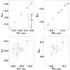 |
Fig. 12. Comparison between the PLZ coefficients obtained with the Lit.+Gaia data set and the Lit. data set. From top-left to bottom-right, the panels show the results for the α, β, γ, and δ coefficients, respectively. For each coefficient, different photometric bands are plotted using different symbols, as labelled in the top-left panel. Grey-filled and empty symbols indicate the fit results including or excluding the δ parameter, respectively. |
5. Discussion
5.1. Parallax correction
A well-known feature of Gaia parallaxes in DR3 is the need for a global offset in the parallaxes after the L21 correction (e.g., Riess et al. 2021, 2022; Molinaro et al. 2023, and references therein). The exact value of this offset is debated and appears to depend on the properties (e.g., location on the sky, magnitude, and colour) and kind of stellar tracer adopted for its estimation (see discussion in Molinaro et al. 2023). To take into account this feature, we also conducted the PLZ/PWZ fit after adding the global offset to the EDR3 parallax values of −14 μas (Riess et al. 2021) or −22 μas (Molinaro et al. 2023). A graphical comparison between these different cases for the Lit.+Gaia sample is shown in Figs. 14 and 15 for the PLZ and PWZ, respectively. The introduction of the parallax correction increases the absolute values of α and β by 1%–4%, while γ decreases monotonically (in an absolute sense) for larger values of the parallax offset. This is particularly visible for the PWZ relations, which show much less scatter than the PLZ ones. In any case, the maximum variation is barely larger than 1σ. The δ coefficient varies less than γ with a slightly decreasing trend; although this latter is insignificant at the 1σ level. Overall, these effects have already been found and are coherent with those discussed in Ripepi et al. (2021a). In practice, the introduction of a significant global parallax zero point offset tends to reconcile our metallicity dependence with typical literature values, as γ tends to diminish with increasing offset (both in an absolute sense). However, as discussed in the following section, the adoption of large offset values affects the absolute distance scale.
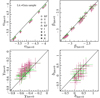 |
Fig. 14. Comparison between the PLZ coefficients obtained for different global offset values. The coefficient values obtained without offset assumption are chosen as reference and are on the x-axis, while those obtained whilst assuming the global parallax offset by Riess et al. (2021) and Molinaro et al. (2023) are on the y-axis and are plotted with green and pink symbols, respectively. From top-left to bottom-right, the panels show the results for the α, β, γ, and δ coefficients, respectively. For each coefficient, different photometric bands are plotted using different symbols, as labelled in the top-left panel, while grey-filled and white-filled symbols indicate the fit results including or excluding the δ parameter, respectively. |
5.2. Distance to the LMC
To test the goodness of our PLZ/PWZ relations and to understand which parameter affects the calibration, we used our relations to estimate the distance to the LMC and compared the results with the currently accepted geometric value μ0 = 18.477 ± 0.026 mag (Pietrzyński et al. 2019). To this aim, we used the method described in detail in Ripepi et al. (2021a). The distance moduli  obtained in this way are listed in Tables 3 and 4 for the Lit.+Gaia and Lit. samples, respectively. The samples including only F pulsators generally give poorer results than the F+1O sample, and therefore in the following discussion we use only the latter data set. Figure 16 shows the resulting
  for the PLZ/PWZ relations for Lit.+Gaia samples. The introduction of the global parallax correction worsens the distance estimation. More precisely, the results with no correction and with Riess et al. (2021) correction are very close to the lower and upper allowed limit, respectively. This suggests for the correction an intermediate value between the two cases, with the exception of
  where Riess et al. (2021) correction perfectly adjusts the value of
  . Therefore, if we use the Pietrzyński et al. (2019) distance of the LMC as a reference, we have to conclude that the rather large values of γ found in this work are favoured over the smaller ones from the recent literature.
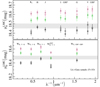 |
Fig. 16. LMC distance modulus obtained using the relations of Table 3 for the F+1O cases plotted against the central wavelength of the considered photometric bands. To avoid labels and symbols overlapping, the I band result has been shifted by −0.1 μm−1. The top panel shows the results for the PLZ relations, while the bottom panel shows those for the PWZ relations. Different colours indicate the results obtained for different parallax shift values: L21 correction (black squares), L21 + Riess et al. (2021) offset (green squares), L21 + Molinaro et al. (2023) (violet squares). Empty and grey-filled squares indicate the results obtained excluding and including the δ coefficient, respectively. |
5.3. Metallicity sampling
Although the results of our C-MetaLL project considerably enlarged the number of DCEPs with [Fe/H] < −0.5 dex, these objects represent less than 10% of the pulsators used in this work, while the majority of the sources are distributed around the solar value. To test whether this unbalanced metallicity distribution could affect our determination of the PLZ/PWZ relations, we conducted an experiment in order to recalculate these relationships by resampling the input data such that its metallicity distribution is uniform over the whole range. To this aim, we divided the sample into five bins in metallicity, imposing the same number of stars in each bin.
As there are few stars in the low-metallicity regime, the sources with [Fe/H] < −0.5 dex were all kept in the same bin and their number, N[FeH < −0.5] = 44 (considering the astrometric selection described in Sect. 2.3), set the number of pulsators included in each of the four remaining bins, whose size is approximately 0.25 dex in metallicity. The DCEPs populating each bin, apart from the lowest metallicity one, were randomly picked. Having resampled the data, we carried out the fit as in Sect. 3 considering the Gaia+Lit. data set only, given that the other cases provide similar results. We also restricted the test to the F+1O sample, because the number of F pulsators in the most metal-poor bin is less than half of the F+1O combined sample, meaning that the total number of DCEPs used for the fit would be too small to achieve meaningful results. We repeated 10 000 times the fitting procedure, obtaining a distribution of values for the α, β, γ, and δ coefficients. Their median values and relative uncertainties (scaled median absolute deviation (MAD)) are compared with the results obtained using the entire sample in Figs. 17 and 18 for PLZ and PWZ, respectively. Both figures show excellent agreement for all of the coefficients. Therefore, we can conclude that the results obtained in this work are not affected by the unbalanced metallicity distribution of the sample.
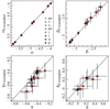 |
Fig. 17. Comparison between the PLZ coefficients obtained with the resampling in metallicity with those obtained using the entire data set. From top-left to bottom-right, the panels show the results for the α, β, γ, and δ coefficients, respectively. For each coefficient, different photometric bands are plotted using different symbols, as labelled in the top-left panel. In contrast, red-filled and white-filled symbols indicate the fit results including or excluding the δ parameter, respectively. |
5.4. Comparison with the literature
Figure 19 shows several empirical estimations of γ throughout the last 20 years. Results from the present work are also plotted, considering the case of the Lit.+Gaia data sample. In more detail, different techniques have been used in order to analyse the metallicity effect on the PL and PW relations. Early studies adopting distances from the Baade–Wesselink (BW) analysis (e.g., Storm et al. 2004, 2011; Groenewegen 2013) reported very small values for the γ parameter in the V, I, and K bands and in the WJK,WVK, and WVI Wesenheit magnitudes. More recently, a stronger effect (γ ∼ −0.2 mag dex−1) – albeit weaker than the effect found in the present work – was found in the same bands by Gieren et al. (2018) from a BW analysis of DCEPs in the Galaxy, LMC, and SMC, which were used to extend the range of metallicity of the pulsators adopted in the analysis.
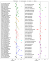 |
Fig. 19. Literature estimation of the γ coefficient for PLZ (left panel) and PWZ (right panel) relations over the last 20 years. Bands are divided by colour and sorted by year of publication from bottom to top. Symbols correspond to the method used to derive the metallicity coefficient. The vertical shaded region corresponds to the range of intervals between −0.4 and −0.2 mag dex−1 (see text for detail). For the complete list of sources, see Fig. 1 from Romaniello et al. (2008) and Table 1 from Breuval et al. (2022). |
The advent of Gaia DR2 parallaxes permitted us to obtain the first reliable evaluation of the γ term using only Galactic DCEPs with metallicities from HiRes spectroscopy. In particular, Groenewegen (2018) and later Ripepi et al. (2019, 2020) found γ ∼ −0.1 − 0.4 mag dex−1 in a variety of bands and Wesenheit magnitudes (see Fig. 19), which is closer to the values found in this paper, but with a significance of generally lower than 1σ, owing to the still insufficient precision of DR2 parallaxes. The improved Gaia EDR3 parallaxes instead allowed us to obtain larger (in an absolute sense) γ values in the first paper of the C-MetaLL project (Ripepi et al. 2021a) and for the WG magnitude (Ripepi et al. 2022).
Other studies (Groenewegen et al. 2004; Fouqué et al. 2007; Wielgórski et al. 2017; Breuval et al. 2021, 2022), together with the already quoted Gieren et al. (2018), compared the properties (i.e., the zero points of the PL or PW relations) of the DCEPs in the MW and in the more metal-poor galaxies LMC and SMC to estimate the extent of the γ value. In particular, Breuval et al. (2021, 2022), used geometric distances for the DCEPs in the MW (from Gaia EDR3 parallaxes) and in the Magellanic Clouds (from eclipsing binaries) to estimate γ in the same bands and Wesenheit magnitudes as those treated in the present work, after fixing the slope of the PL and PW relations to that of the LMC, with results ranging between −0.178 and −0.462 mag dex−1. In the context of the SH0ES project (Riess et al. 2016, 2019, 2021, 2022), the metallicity effect is one of the outputs of the process for the estimation of H0. In these cases, the γ coefficient in the  magnitude used by the SH0ES team is of the order of −0.2 mag dex−1, while we obtain a slightly larger (in an absolute sense) value in our best case, that is, with the Lit.+Gaia sample without the δ term (see e.g., Fig. 5).
Recent theoretical studies (Anderson et al. 2016; De Somma et al. 2022) also predict mild effects of the metallicity, with γ ranging from −0.27 to −0.13 mag dex−1, although we note that the models by De Somma et al. (2022) only deal with PW relations.
We notice that in almost all cases, we find larger γ values (in an absolute sense) than the literature, although most of them are distributed along the lower limit in the literature of −0.4 mag dex−1 (see also Fig. 4). On the other side, for the V-band a smaller coefficient is found, in agreement with the upper limit of −0.2 mag dex−1.
6. Conclusion
In this fourth paper of the C-MetaLL series, we studied the metallicity dependence of the PL relations in the following bands: GBP, GRP, G, I, V, J, H, and KS, and of the PW relations in the following Wesenheit magnitudes:  ,WJ, J − K, and WV, V − K. To this end, we exploited the literature to compile a sample of 910 DCEPs with [Fe/H] measured from HiRes spectroscopy and complemented it with a number of stars with metallicity measurements based on the Gaia RVS instrument as released in DR3. For all these stars, we provide a table with photometry in the GBP, GRP, G, I, V, J, H, and KS bands, metallicity, and astrometry from Gaia DR3.
We carried out our analysis adopting two different samples: one composed only of literature data and one including both the latter and Gaia DR3 results. In order to estimate the parameters of the PLZ/PWZ relations, we used the ABL formalism, which allowed us to treat the parallax ϖ linearly and to preserve the statistical properties of its uncertainties. We considered two functional forms for the PLZ and PWZ relations including (i) the metallicity dependence on the intercept only (three-parameter case); and (ii) the metallicity dependence on both intercept and slope (four-parameter case). The main findings of our analysis can be summarised as follows:
-
Regarding PLZ relations, both α and β show a linear dependence on wavelength. We provide the linear relationships between these quantities and λ−1. These relations do not change considerably when we use the Lit.+Gaia or Lit. samples, nor when we carry out a three- or four-parameter fit. Because of the low wavelength coverage, no clear dependence can be discussed for the PWZ relations.
-
A clear negative dependence of the intercept on metallicity (γ-coefficient) is found for all the PL and PW relations. For the three-parameter solutions, the values of γ are around −0.4 : −0.5 dex with no clear dependence on wavelength. Thus, this work confirms our previous results reported by Ripepi et al. (2021a); Molinaro et al. (2023). For the four-parameter solutions, the values of γ generally slightly decrease (in an absolute sense), especially for the Lit. only sample. In general, the γ coefficients found in this work are larger (in an absolute sense) than those in the literature, which range between −0.2 and −0.4 dex.
-
The dependence of the slope on metallicity (δ coefficient) remains undetermined. Indeed, in about half of the cases, δ assumes values comparable with zero within 1σ for the Gaia+Lit. sample, while, especially in the Lit. case, δ generally assumes a positive value comprised between 0 and +0.5.
-
The main difference between using the F and F+1O samples is that larger error bars are found in the former case, especially for the γ and δ coefficients.
-
The inclusion of global zero point offset to the individually corrected parallaxes according to L21 has a larger impact on the γ coefficients than on the δ ones. More specifically, the adoption of offsets by −14 μas (Riess et al. 2021) and −22 μas (Molinaro et al. 2023) implicates smaller and smaller values of γ (in an absolute sense), which is in better agreement with recent literature. However, if we use the geometric distance of the LMC by Pietrzyński et al. (2019) as a reference and calculate the distance of this galaxy using our relations with and without the global offset, we find that good agreement for the distance of the LMC is found for values of the offset in between null and the 14 μas values. It is worth noting that for the
 magnitude Riess et al. (2021) offset represents the best correction. These results support larger values (in an absolute sense) of the γ value.
 -
We investigated the possible effect of an uneven distribution in the metallicity of the sample used in this work by resampling our data set in order to have a balanced number of DCEPs at every metallicity value. We carried out the fitting procedure on 10 000 samples extracted from the total sample, obtaining a value for the four coefficients of the fit for every data set. The medians of the obtained distributions for all the coefficients appear to be in excellent agreement with those obtained using the entire sample. Therefore, we can conclude that the results obtained in this work are not affected by the sample’s unbalanced distribution in metallicity.
The results presented in this paper show the importance of the extension of the metallicity range when carrying out the analysis. Further observations in order to gather HiRes spectroscopy of MW metal-poor DCEPs will offer the opportunity to better constrain the dependence on the metallicity of both the intercept and the slope. In particular, regions in the Galactic anti-centre direction are the most promising targets for future observations, where DCEPs are expected to have [Fe/H] < −0.3 : −0.4 dex, and can therefore be used to further populate the metal-poor tail of the DCEP distribution.
Supernovae, HO, for the Equation of State of Dark energy.
The Wesenheit magnitudes introduced by Madore (1982) provide a reddening-free magnitude by supposing that the adopted extinction law does not change significantly from star to star as can happen if the targets are placed in regions of the Galaxy with different chemical enrichment histories.
The I photometry is in the Cousins system.
We caution the reader that the conversion equations in Riess et al. (2021) contain a typo regarding the F814W filter. In this work we used the correct relation F814W = V − 0.48(V − H)−0.025 instead of F814W = V − 0.48(J − H)−0.025
Acknowledgments
We thank our anonymous Referee for their helpful comments which helped us to improve the paper. Part of this work was supported by the German Deutsche Forschungsgemeinschaft, DFG project number Ts 17/2–1. This work has made use of data from the European Space Agency (ESA) mission Gaia (https://www.cosmos.esa.int/gaia), processed by the Gaia Data Processing and Analysis Consortium (DPAC, https://www.cosmos.esa.int/web/gaia/dpac/consortium). Funding for the DPAC has been provided by national institutions, in particular, the institutions participating in the Gaia Multilateral Agreement. This research has made use of the VizieR catalogue access tool, CDS, Strasbourg, France. This research has made use of the SIMBAD database, operated at CDS, Strasbourg, France. I.M. acknowledges partial financial support by INAF, Minigrant “Are the Ultra Long Period Cepheids cosmological standard candles?” We acknowledge funding from INAF GO-GTO grant 2023 “C-MetaLL – Cepheid metallicity in the Leavitt law” (P.I. V. Ripepi)
References
- Alcock, C., Allsman, R. A., Axelrod, T. S., et al. 1995, AJ, 109, 1653 [NASA ADS] [CrossRef] [Google Scholar]
- Anderson, R. I., Casertano, S., Riess, A. G., et al. 2016, ApJS, 226, 18 [NASA ADS] [CrossRef] [Google Scholar]
- Arenou, F., & Luri, X. 1999, in Harmonizing Cosmic Distance Scales in a Post-HIPPARCOS Era, eds. D. Egret, & A. Heck, ASP Conf. Ser., 167, 13 [NASA ADS] [Google Scholar]
- Bono, G., Caputo, F., Marconi, M., & Musella, I. 2010, ApJ, 715, 277 [Google Scholar]
- Breuval, L., Kervella, P., Wielgórski, P., et al. 2021, ApJ, 913, 38 [NASA ADS] [CrossRef] [Google Scholar]
- Breuval, L., Riess, A. G., Kervella, P., Anderson, R. I., & Romaniello, M. 2022, ApJ, 939, 89 [NASA ADS] [CrossRef] [Google Scholar]
- Brodie, J. P., & Madore, B. F. 1980, MNRAS, 191, 841 [NASA ADS] [CrossRef] [Google Scholar]
- Buder, S., Sharma, S., Kos, J., et al. 2021, MNRAS, 506, 150 [NASA ADS] [CrossRef] [Google Scholar]
- Caputo, F., Marconi, M., Musella, I., & Santolamazza, P. 2000, A&A, 359, 1059 [NASA ADS] [Google Scholar]
- Cardelli, J. A., Clayton, G. C., & Mathis, J. S. 1989, ApJ, 345, 245 [Google Scholar]
- Catanzaro, G., Ripepi, V., Clementini, G., et al. 2020, A&A, 639, L4 [NASA ADS] [CrossRef] [EDP Sciences] [Google Scholar]
- Chen, X., Wang, S., Deng, L., et al. 2020, ApJS, 249, 18 [NASA ADS] [CrossRef] [Google Scholar]
- Clementini, G., Ripepi, V., Molinaro, R., et al. 2019, A&A, 622, A60 [NASA ADS] [CrossRef] [EDP Sciences] [Google Scholar]
- De Somma, G., Marconi, M., Molinaro, R., et al. 2022, ApJS, 262, 25 [NASA ADS] [CrossRef] [Google Scholar]
- Feast, M. W., & Catchpole, R. M. 1997, MNRAS, 286, L1 [NASA ADS] [CrossRef] [Google Scholar]
- Fiorentino, G., Musella, I., & Marconi, M. 2013, MNRAS, 434, 2866 [Google Scholar]
- Fouqué, P., Arriagada, P., Storm, J., et al. 2007, A&A, 476, 73 [NASA ADS] [CrossRef] [EDP Sciences] [Google Scholar]
- Freedman, W. L., Madore, B. F., Scowcroft, V., et al. 2012, ApJ, 758, 24 [Google Scholar]
- Gaia Collaboration (Prusti, T., et al.) 2016, A&A, 595, A1 [NASA ADS] [CrossRef] [EDP Sciences] [Google Scholar]
- Gaia Collaboration (Clementini, G., et al.) 2017, A&A, 605, A79 [NASA ADS] [CrossRef] [EDP Sciences] [Google Scholar]
- Gaia Collaboration (Brown, A. G. A., et al.) 2018, A&A, 616, A1 [NASA ADS] [CrossRef] [EDP Sciences] [Google Scholar]
- Gaia Collaboration (Brown, A. G. A., et al.) 2021, A&A, 649, A1 [NASA ADS] [CrossRef] [EDP Sciences] [Google Scholar]
- Genovali, K., Lemasle, B., Bono, G., et al. 2014, A&A, 566, A37 [NASA ADS] [CrossRef] [EDP Sciences] [Google Scholar]
- Gieren, W., Storm, J., Konorski, P., et al. 2018, A&A, 620, A99 [NASA ADS] [CrossRef] [EDP Sciences] [Google Scholar]
- Groenewegen, M. 2013, A&A, 550, A70 [NASA ADS] [CrossRef] [EDP Sciences] [Google Scholar]
- Groenewegen, M. A. T. 2018, A&A, 619, A8 [NASA ADS] [CrossRef] [EDP Sciences] [Google Scholar]
- Groenewegen, M. A. T., Romaniello, M., Primas, F., & Mottini, M. 2004, A&A, 420, 655 [NASA ADS] [CrossRef] [EDP Sciences] [Google Scholar]
- Kovtyukh, V., Lemasle, B., Bono, G., et al. 2022, MNRAS, 510, 1894 [Google Scholar]
- Leavitt, H. S., & Pickering, E. C. 1912, Harvard College Obs. Circ., 173, 1 [NASA ADS] [Google Scholar]
- Lemasle, B., Lala, H. N., Kovtyukh, V., et al. 2022, A&A, 668, A40 [NASA ADS] [CrossRef] [EDP Sciences] [Google Scholar]
- Lindegren, L., Bastian, U., Biermann, M., et al. 2021, A&A, 649, A4 [EDP Sciences] [Google Scholar]
- Luck, R. E. 2018, AJ, 156, 171 [Google Scholar]
- Madore, B. F. 1982, ApJ, 253, 575 [NASA ADS] [CrossRef] [Google Scholar]
- Madore, B. F., & Freedman, W. L. 2011, ApJ, 744, 132 [Google Scholar]
- Marconi, M., Musella, I., & Fiorentino, G. 2005, ApJ, 632, 590 [Google Scholar]
- Marconi, M., Musella, I., Fiorentino, G., et al. 2010, ApJ, 713, 615 [NASA ADS] [CrossRef] [Google Scholar]
- Molinaro, R., Ripepi, V., Marconi, M., et al. 2023, MNRAS, 520, 4154 [NASA ADS] [CrossRef] [Google Scholar]
- Montegriffo, P. 2023, A&A, 674, A33 [CrossRef] [EDP Sciences] [Google Scholar]
- Pancino, E., Marrese, P. M., Marinoni, S., et al. 2022, A&A, 664, A109 [NASA ADS] [CrossRef] [EDP Sciences] [Google Scholar]
- Pietrzyński, G., Graczyk, D., Gallenne, A., et al. 2019, Nature, 567, 200 [Google Scholar]
- Planck Collaboration VI. 2020, A&A, 641, A6 [NASA ADS] [CrossRef] [EDP Sciences] [Google Scholar]
- Recio-Blanco, A., de Laverny, P., Palicio, P. A., et al. 2023, A&A, 674, A29 [NASA ADS] [CrossRef] [EDP Sciences] [Google Scholar]
- Riess, A. G., Macri, L. M., Hoffmann, S. L., et al. 2016, ApJ, 826, 56 [Google Scholar]
- Riess, A. G., Casertano, S., Yuan, W., Macri, L. M., & Scolnic, D. 2019, ApJ, 876, 85 [Google Scholar]
- Riess, A. G., Casertano, S., Yuan, W., et al. 2021, ApJ, 908, L6 [NASA ADS] [CrossRef] [Google Scholar]
- Riess, A. G., Yuan, W., Macri, L. M., et al. 2022, ApJ, 934, L7 [NASA ADS] [CrossRef] [Google Scholar]
- Ripepi, V., Molinaro, R., Musella, I., et al. 2019, A&A, 625, A14 [NASA ADS] [CrossRef] [EDP Sciences] [Google Scholar]
- Ripepi, V., Catanzaro, G., Molinaro, R., et al. 2020, A&A, 642, A230 [NASA ADS] [CrossRef] [EDP Sciences] [Google Scholar]
- Ripepi, V., Catanzaro, G., Molinaro, R., et al. 2021a, MNRAS, 508, 4047 [NASA ADS] [CrossRef] [Google Scholar]
- Ripepi, V., Catanzaro, G., Molnár, L., et al. 2021b, A&A, 647, A111 [NASA ADS] [CrossRef] [EDP Sciences] [Google Scholar]
- Ripepi, V., Catanzaro, G., Clementini, G., et al. 2022, A&A, 659, A167 [NASA ADS] [CrossRef] [EDP Sciences] [Google Scholar]
- Romaniello, M., Primas, F., Mottini, M., et al. 2008, A&A, 488, 731 [NASA ADS] [CrossRef] [EDP Sciences] [Google Scholar]
- Rybizki, J., Green, G. M., Rix, H.-W., et al. 2022, MNRAS, 510, 2597 [NASA ADS] [CrossRef] [Google Scholar]
- Sandage, A., & Tammann, G. A. 2006, ARA&A, 44, 93 [NASA ADS] [CrossRef] [Google Scholar]
- Skrutskie, M. F., Cutri, R. M., Stiening, R., et al. 2006, AJ, 131, 1163 [NASA ADS] [CrossRef] [Google Scholar]
- Soubiran, C., Le Campion, J.-F., Brouillet, N., & Chemin, L. 2016, A&A, 591, A118 [NASA ADS] [CrossRef] [EDP Sciences] [Google Scholar]
- Storm, J., Carney, B. W., Gieren, W. P., et al. 2004, A&A, 415, 521 [NASA ADS] [CrossRef] [EDP Sciences] [Google Scholar]
- Storm, J., Gieren, W., Fouqué, P., et al. 2011, A&A, 534, A94 [CrossRef] [EDP Sciences] [Google Scholar]
- Tammann, G. A., Sandage, A., & Reindl, B. 2003, A&A, 404, 423 [NASA ADS] [CrossRef] [EDP Sciences] [Google Scholar]
- Trentin, E., Ripepi, V., Catanzaro, G., et al. 2023, MNRAS, 519, 2331 [Google Scholar]
- Udalski, A., Soszyński, I., Pietrukowicz, P., et al. 2018, Acta Astron., 68, 315 [Google Scholar]
- van Leeuwen, F., Feast, M. W., Whitelock, P. A., & Laney, C. D. 2007, MNRAS, 379, 723 [NASA ADS] [CrossRef] [Google Scholar]
- Wielgórski, P., Pietrzyński, G., Gieren, W., et al. 2017, ApJ, 842, 116 [CrossRef] [Google Scholar]
Appendix A: PLZ/PWZ coefficients for the F pulsators only sample
For completeness, we provide figures that are analogous to Fig. 4, Fig. 5, Fig. 10, and Fig. 11, showing the fit results of the sample Lit.+Gaia and Lit. including only the F pulsators.
Appendix B: Parallax correction for the Lit. sample
Here, we provide figures analogues to Fig. 14, Fig. 15, and Fig. 16 for the Lit. sample.
All Tables
Photometric, astrometric, and spectroscopic data for the DCEP sample used in this work.
Photometric bands and colour coefficients adopted to calculate the Wesenheit magnitudes considered in this work.
All Figures
|
Fig. 1. Comparison between the literature V, I photometry and that from Gaia through the transformation by Pancino et al. (2022). The top and bottom panels show the comparison in V and I bands, respectively. |
| In the text | |
|
Fig. 2. Comparison between the [Fe/H] from HiRes data and Gaia [M/H]. From top to bottom, the different panels show the comparison for the low-, medium-, and high-quality Gaia data, respectively (see text for details). In each panel, the average difference Δ and its dispersion is displayed. |
| In the text | |
|
Fig. 3. Individual parallax corrections from L21 as a function of the G magnitude. The points are colour coded according to the ecliptic latitude. |
| In the text | |
|
Fig. 4. Coefficients of PLZ/PWZ relations obtained from the fit to the Lit.+Gaia sample plotted against the λ−1 parameter. From top to bottom, the panels correspond to the α, β, γ, and δ coefficients. In each panel, PLZ and PWZ coefficients are plotted with blue and red symbols respectively, while the solid line shows the linear fit only for the PLZ relations. Grey dashed lines in the γ panel delimit the range of results in the literature (−0.2 to −0.4 mag dex−1, see Breuval et al. 2022, and Sect. 5.4), while in the δ panel, it corresponds to the value 0. |
| In the text | |
|
Fig. 5. Same as Fig. 4 but for the case neglecting the metallicity dependence in the PLZ/PLW slope (i.e., δ = 0). |
| In the text | |
|
Fig. 6. PL relations for the bands studied in the paper where the magnitudes have been subtracted by the metallicity contribution. The colour bar represents the metallicity. |
| In the text | |
|
Fig. 7. Visualization of the PL dependence on the metallicity. The y-axis is the magnitudes subtracted by the period contribution and the x-axis is the metallicity. The colour bar represents the logarithm of the period. |
| In the text | |
 |
Fig. 8. Same as Fig. 6 but for the PWZ relations. |
| In the text | |
 |
Fig. 9. Same as Fig. 7 but for the PWZ relations. |
| In the text | |
 |
Fig. 10. Same as Fig. 4 but for the Lit. sample. |
| In the text | |
 |
Fig. 11. Same as Fig. 5 but for the Lit. sample. |
| In the text | |
|
Fig. 12. Comparison between the PLZ coefficients obtained with the Lit.+Gaia data set and the Lit. data set. From top-left to bottom-right, the panels show the results for the α, β, γ, and δ coefficients, respectively. For each coefficient, different photometric bands are plotted using different symbols, as labelled in the top-left panel. Grey-filled and empty symbols indicate the fit results including or excluding the δ parameter, respectively. |
| In the text | |
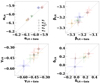 |
Fig. 13. Same as Fig. 12 but for the PWZ relations. |
| In the text | |
|
Fig. 14. Comparison between the PLZ coefficients obtained for different global offset values. The coefficient values obtained without offset assumption are chosen as reference and are on the x-axis, while those obtained whilst assuming the global parallax offset by Riess et al. (2021) and Molinaro et al. (2023) are on the y-axis and are plotted with green and pink symbols, respectively. From top-left to bottom-right, the panels show the results for the α, β, γ, and δ coefficients, respectively. For each coefficient, different photometric bands are plotted using different symbols, as labelled in the top-left panel, while grey-filled and white-filled symbols indicate the fit results including or excluding the δ parameter, respectively. |
| In the text | |
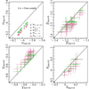 |
Fig. 15. Same as Fig. 14 but for the PWZ coefficients. |
| In the text | |
|
Fig. 16. LMC distance modulus obtained using the relations of Table 3 for the F+1O cases plotted against the central wavelength of the considered photometric bands. To avoid labels and symbols overlapping, the I band result has been shifted by −0.1 μm−1. The top panel shows the results for the PLZ relations, while the bottom panel shows those for the PWZ relations. Different colours indicate the results obtained for different parallax shift values: L21 correction (black squares), L21 + Riess et al. (2021) offset (green squares), L21 + Molinaro et al. (2023) (violet squares). Empty and grey-filled squares indicate the results obtained excluding and including the δ coefficient, respectively. |
| In the text | |
|
Fig. 17. Comparison between the PLZ coefficients obtained with the resampling in metallicity with those obtained using the entire data set. From top-left to bottom-right, the panels show the results for the α, β, γ, and δ coefficients, respectively. For each coefficient, different photometric bands are plotted using different symbols, as labelled in the top-left panel. In contrast, red-filled and white-filled symbols indicate the fit results including or excluding the δ parameter, respectively. |
| In the text | |
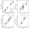 |
Fig. 18. Same as Fig. 17, but for the PWZ coefficients. |
| In the text | |
|
Fig. 19. Literature estimation of the γ coefficient for PLZ (left panel) and PWZ (right panel) relations over the last 20 years. Bands are divided by colour and sorted by year of publication from bottom to top. Symbols correspond to the method used to derive the metallicity coefficient. The vertical shaded region corresponds to the range of intervals between −0.4 and −0.2 mag dex−1 (see text for detail). For the complete list of sources, see Fig. 1 from Romaniello et al. (2008) and Table 1 from Breuval et al. (2022). |
| In the text | |
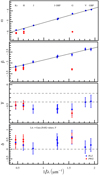 |
Fig. A.1. Same as Fig. 4 but for the Lit.+Gaia data set including only F pulsators. |
| In the text | |
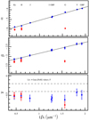 |
Fig. A.2. Same as Fig. 5 but for the Lit.+Gaia data set including only F pulsators. |
| In the text | |
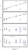 |
Fig. A.3. Same as Fig. 10 but for the Lit. data set including only F pulsators. |
| In the text | |
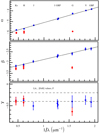 |
Fig. A.4. Same as Fig. 11 but for the Lit. data set including only F pulsators. |
| In the text | |
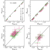 |
Fig. B.1. Same as Fig. 14 but for the Lit. sample. |
| In the text | |
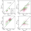 |
Fig. B.2. Same as Fig. 15 but for the Lit. sample. |
| In the text | |
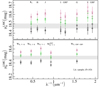 |
Fig. B.3. Same as Fig. 16 but for the Lit. sample. |
| In the text | |
Current usage metrics show cumulative count of Article Views (full-text article views including HTML views, PDF and ePub downloads, according to the available data) and Abstracts Views on Vision4Press platform.
Data correspond to usage on the plateform after 2015. The current usage metrics is available 48-96 hours after online publication and is updated daily on week days.
Initial download of the metrics may take a while.