A deep Hα survey of the Carina tangent arm direction

D. Russeil; A. Zavagno; P. Amram; D. Elia; S. Molinari; E. Lecoarer

doi:10.1051/0004-6361/202346973

Home

All issues

Volume 680 (December 2023)

A&A, 680 (2023) A81

Full HTML

Open Access

Issue		A&A Volume 680, December 2023


Article Number		A81
Number of page(s)		26
Section		Galactic structure, stellar clusters and populations
DOI		https://doi.org/10.1051/0004-6361/202346973
Published online		18 December 2023

A&A 680, A81 (2023)

A deep Hα survey of the Carina tangent arm direction^⋆

D. Russeil¹, A. Zavagno¹, P. Amram¹, D. Elia², S. Molinari² and E. Lecoarer³

¹ Aix-Marseille Univ., CNRS, CNES, LAM, 13388 Marseille, France
e-mail: delphine.russeil@lam.fr
² INAF-IAPS, Via Fosso del Cavaliere 100, 00133 Roma, Italy
³ Univ. Grenoble Alpes, CNRS, IPAG, 38000 Grenoble, France

Received: 23 May 2023
Accepted: 30 September 2023

Abstract

Aims. The arm tangent direction provides a unique viewing geometry, with a long path in relatively narrow velocity ranges and lines of view that cross the arm perpendicular to its thickness. The spiral arm tangent regions are therefore the best directions for studying the interstellar medium within spiral density waves in the Milky Way, probing the internal structure in the arms. We focus here on the gas kinematics and star formation in the Galactic plane zone with longitudes of between 281° and 285.5° and latitudes of between ∼−2.5° and ∼1°, respectively, which contains the Carina arm tangency.

Methods. The Carina arm tangent direction was observed as part of a velocity-resolved Hα survey of the southern Milky Way using a scanning Fabry-Perot mounted on a telescope, which makes it possible to obtain data cubes containing kinematic information. Our detailed analysis of the resultant Hα profiles reveals the presence of several layers of ionized gas with different velocities over the surveyed region. We combine the Hα data with multi-wavelength information in order to assign velocity and distance to the H II regions in the probed area and to study the star-formation activity in the Carina arm tangency.

Results. We find that the Carina arm tangency is at l = 282°, and that it spreads from 2 to 6 kpc with a V_LSR range of between −20 and +20 km s⁻¹. We deduce an arm width of ∼236 pc. We also probe the star formation on a scale of ∼1 kpc⁻², showing that the star-formation activity is intermediate in comparison with the quiescient Solar neighborhood and the most active Galactic central molecular zone. From our analysis of the stellar motions extracted from the Gaia DR3 catalog, we observe that stars around 2.5 kpc are tracing the trailing and the leading sides of the arm, while stars at greater distances more closely trace the inner part of the arm. In parallel, we studied the Hα velocity structure of the H II regions RCW48 and RCW49 in detail, confirming the expansion velocity of ∼20 km s⁻¹ for RCW 49 and the double-shell structure of RCW 48, which is in agreement with a wind interaction with a previous mass-loss episode.

Key words: stars: kinematics and dynamics / H II regions

^⋆

The data cubes are available at the CDS via anonymous ftp to cdsarc.cds.unistra.fr (130.79.128.5) or via https://cdsarc.cds.unistra.fr/viz-bin/cat/J/A+A/680/A81

© The Authors 2023

Open Access article, published by EDP Sciences, under the terms of the Creative Commons Attribution License (https://creativecommons.org/licenses/by/4.0), which permits unrestricted use, distribution, and reproduction in any medium, provided the original work is properly cited.

This article is published in open access under the Subscribe to Open model. Subscribe to A&A to support open access publication.

1. Introduction

The arm tangent direction provides a unique viewing geometry, with a long path length in relatively narrow velocity ranges and lines of view that cross the arm perpendicular to its thickness. The spiral arm tangent regions are therefore the best directions for studying the interstellar medium within spiral density waves in the Milky Way, probing the internal structure in the arms by locating the emission lanes within them (e.g., Velusamy et al. 2015).

The Carina arm is a major Galactic arm in the sense that it is richly populated by bright H II regions (e.g., the Carina nebula), but its tangent direction is not prominent in any surface density – longitude plots (Hou & Han 2015). In particular, it is not seen at all on near- or mid-infrared source (old stars) counts (see Fig. 2 in Hou & Han 2015), which led Benjamin et al. (2005) – who based their study on Spitzer/GLIMPSE mid-infrared star counts – to report only two major stellar arms, the Perseus arm and the Scutum-Centaurus arm. In this frame, the two other arms, the Sagittarius-Carina and the Norma arms, can be considered to be mainly gaseous, with a few old stars. In parallel, in the fourth Galactic quadrant (l = 270°–360°), Russeil (2003) underlined that the Norma Arm is clearly seen in far-infrared, while the Crux (Centaurus) arm stands out clearly in molecular emission, and the Carina arm is the weakest. However, Elia et al. (2021), based on the Hi-GAL clumps survey, found no striking differences in median evolutionary stage across different Galactocentric radii, and/or in correspondence with spiral arms, whose role seems not to be crucial for triggering star formation, but rather for gathering matter.

The sector of the Galaxy at the tangent direction of the Carina arm, around l = 282° (Vallée 2008), is poorly studied because the extinction is particularly strong and variable, but also because kinematical interpretation is difficult. Indeed, because the tangent direction of the Carina arm falls close to the Solar circle (it cuts it around l = 282°), the velocities are not well separated from the local emission at V_LSR around 0 km s⁻¹, but also any departure from circular rotation (random and systematic noncircular motions such as the velocity dispersion of molecular clouds and the streaming motion along the arms) leads sources either to have forbidden V_LSR and then no kinematic distance determination or to pass at positive velocity, which places them erroneously at the far distance. In addition, in this direction, the atomic hydrogen gas (Levine et al. 2006), the molecular clouds, and the ionized gas are found below the Galactic plane (e.g., Cohen et al. 1985; Grabelsky et al. 1987; Cersosimo et al. 2009), tracing the warp descending from z ∼ −10 to −150 pc between Galactic radii of R ∼ 7.3 and 9.7 kpc (Cersosimo et al. 2009). Finally, Naoz & Shaviv (2007) suggest that the Carina arm is a superposition of two arms with two different pattern speeds with the slower one being more prominent.

To better understand the kinematics and star formation in the Carina tangent direction, we carried out a detailed analysis of the ionized gas (diffuse emission as well as discrete H II regions) kinematics as observed in the Hα line. Coupled with multiwavelength data, we present and use the archival data from the Hα survey of the southern Milky Way, which was carried out with a 36 cm telescope in La Silla equipped with a scanning Fabry-Perot and a photon counting camera (Amram et al. 1991; Le Coarer et al. 1992).

The paper is organized as follows: we present the data in Sect. 2, and the Hα data are analyzed in Sect. 3, focusing mainly on the Hα kinematics of the H II regions. We characterize the Carina arm tangent direction in Sects. 4 and 5, and discuss the star formation activity in Sects. 6 and 7.

2. Data

2.1. Hα observations

Hα line data cubes (x, y, λ) were obtained (pixel size 9″) for 20 fields (39′×39′ each) in the direction around 283° longitude and −1° latitude. The observations were performed from 1992 to 1994. The instrument is now decommissioned. Figure 1 shows the mosaic of observed fields where H II regions as well as patchy diffuse Hα emission can be seen. A complete description of the instrument, including data acquisition and reduction techniques, can be found in Le Coarer et al. (1992). Two different Fabry-Perot interferometers (interference orders P = 2604 or P = 796, at 6562.8 Å, the Hα wavelength) were used depending on the anticipated velocity range covered by the observed structures. At Hα at rest, the interferometers provide a resolving power of ∼30 000 and 10 000, respectively. Adhering to spectral sampling principles, we used a spectral sampling of 5 km s ⁻¹ and 16 km s ⁻¹ for a spectral range of 115 km s ⁻¹ and 376 km s ⁻¹, respectively (most of the fields were observed with the P = 2604 interferometer). The interference filter used is centered at 6562 Å with a full width at half maximum (FWHM) of 11 Å. The data are not flux calibrated: the intensity unit is events counted by the photon-counting camera per pixel per hour (evt./px/h). Data reduction follows the procedures described in Georgelin et al. (1994). The velocity is in the local standard of rest (LSR) and the typical velocity uncertainty (estimated following Lenz & Ayres 1992) is 2 km s⁻¹. The night-sky lines (geocoronal Hα and OH) are modeled by the instrumental function (obtained using neon lamp line observations), while the nebular lines are modeled by Gaussian profiles convolved with the instrumental function.

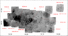Fig. 1.

General view of the covered area (the J2000 coordinates are in h:m and °:′ format, respectively). This Hα image is a mosaic of the images obtained by adding all the planes of the observed datacubes. The contrast has been chosen to highlight the diffuse emission structures. The names of the main optical H II regions are given in red.

The major difficulty is in disentangling line-of-sight intensity components found in the complex observed Hα line profile. Inside a given field, we can distinguish three or even four main galactic components (in addition to the geocoronal Hα and OH nightsky lines) with each corresponding to a different layer of ionized hydrogen. Generally, the different components exhibit similar velocity all over the observed field, which enables us to follow them rather easily despite their highly varying intensity.

2.2. Other data sets

In addition to the Hα data, we used the HI4PI and the ¹²CO(1–0) NANTEN datacubes as well as the Hi-GAL column-density map. The HI4PI (HI4PI Collaboration 2016) is a full-sky survey of the H I 21 cm line combining the Effelsberg-Bonn HI Survey (EBHIS) and the Galactic All-Sky Survey (GASS). The datacube used has a velocity resolution and coverage of 1.28 km s⁻¹ and ∼1200 km s⁻¹, respectively, with a spatial resolution of 5′. In addition, we retrieved the delivered H I column density (N_HI) maps integrated over different velocity ranges (especially the one integrated from −20 to +20 km s⁻¹). The ¹²CO(1–0) NANTEN velocity cube (Mizuno et al. 2004) used has a velocity resolution and coverage of 1 km s⁻¹ and ∼300 km s⁻¹, respectively, with a pixel size of 4′. The Hi-GAL project (Molinari et al. 2010) is a photometric survey of the entire Galactic plane with the Herschel Space Observatory (Pilbratt et al. 2010) in the wavelength range from 70 to 500 μm, from which H₂ column-density (N_H₂) maps have been derived (Elia et al. 2013; Schisano et al. 2020). The N_H₂ map used here has a spatial resolution of 36″.

To investigate the extinction, we retrieved the A_V and A_Ks extinction maps¹ (Dobashi et al. 2005, 2013; Dobashi 2011). The A_V and A_Ks maps used have pixel sizes of 2′ and 1′, respectively. The A_V and A_Ks extinctions are measured using an upgraded version of the technique called the near-infrared color excess method (NICE) applied to the 2MASS point-source catalog (Dobashi 2011) and to the optical photographic database DSS (Dobashi et al. 2005) catalog, respectively, and are corrected for background (Dobashi et al. 2013).

3. Hα data analysis

In the following, the kinematic distance (d_kin) is calculated from the Russeil et al. (2017) rotation curve. If the velocity is forbidden, one can then adopt the tangent distance, denoted d_tan. The adopted rotation curve assumes a Sun to Galactic center distance (R₀) of 8.34 kpc and a rotation velocity (θ₀) of 240 km s⁻¹. For the longitudes probed in this paper, using this rotation curve leads, on average, to overestimation of the kinematic distance by 0.9 kpc, 0.9 kpc, 0.8 kpc, and 0.7 kpc with respect to the findings of Bovy et al. (2012), Eilers et al. (2019), Mróz et al. (2019), and Wang et al. (2023) with their rotation curves, respectively. However, these more recent rotation curves are established from different samples, with different sample coverage, and for different R₀ (between 8.0 and 8.34 kpc) and different θ₀ (between 218 and 299 km s⁻¹). For stars, the parallactic distance (d_Gaia) is either the one from the Bailer-Jones et al. (2021) catalog (1″ cone search cross-correlation) or the one calculated using the TOPCAT functions “distanceEstimateEdsd” and “distanceBoundsEdsd”. These functions calculate from the parallax the best estimate of distance and the 5th and 95th percentile confidence intervals using an exponentially decreasing space density prior (adopting a length scale of 1500 pc). We can note that stars with RUWE² ≤ 1.4 and π/σ_π > 5 can be considered as having a more reliable distance estimate. The photometric distance (d_phot) of a star is estimated from the spectra and/or UBV photometry (retrieved from the CDS³) following Russeil et al. (2007).

3.1. Diffuse emission and extinction

Figure 2 presents the velocities measured from profile decomposition. From this figure, in addition to the structured H II regions, three extended diffuse emissions are observed. The first emission has a mean velocity of −3.8 km s⁻¹ (between −0.5 and −9 km s⁻¹) observed all over the field. Its intensity is very variable (between 1 and 16 evt./px/h) even through a single elementary field of the mosaic. Most of the Hα diffuse structures and H II regions also display this velocity. The relatively large velocity and intensity ranges can be explained by considering that, at this velocity, we cannot distinguish the spiral arm diffuse emission from the local arm emission as observed in the other fields (e.g., Russeil et al. 1998).

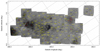Fig. 2.

Velocity components (the Galactic coordinate axes are displayed in the figure). The LSR velocity (in km s⁻¹) of the different components is given in yellow (and sorted by decreasing peak intensity). The typical velocity uncertainty is 2 km s⁻¹. For the brightest parts of the H II regions, only the main and intensity-dominating component is given in red (in blue if this component is very broad with FWHM ≥ 40 km s⁻¹).

The second diffuse layer has a mean velocity of −23 km s⁻¹ (between −19 and −29 km s⁻¹) and is also observed all over the mosaic. Its intensity is relatively constant (∼1.1 evt./px/h), except around GUM30, where it reaches 5 evt./px/h. Several H II regions can be associated to this layer: GUM30, GUM31 (outside the mosaic), and the Carina nebula (outside the mosaic). Because this velocity is forbidden, d_kin cannot be calculated; however, we can assume a distance of ∼2.3 kpc for this layer based on the distance of the Carina nebula given by Shull et al. (2021) and the conclusions of Georgelin et al. (2000).

The third diffuse layer has a mean velocity of +12.1 km s⁻¹; it is largely present in the mosaic except in its northwest part (see Fig. 2). This suggests that this diffuse emission is farther (with a d_kin ∼ 6 kpc) and therefore more strongly absorbed. Its mean intensity is 0.9 evt./px/h, except between RCW48 and RCW49, where it reaches 3 evt./px/h.

To investigate the large-scale morphology of the extinction, we look at the A_V and A_Ks extinction maps from Dobashi et al. (2013). Figure 3 shows that the extinction is stronger in an area of ∼0.8° radius centered around l, b = 281.7°, −0.9° (α,δ = 10h15min, −57°30′) and that most of the mosaic, especially RCW 48 and RCW 49, are located in an area of moderate extinction (A_V between 1 and 2 mag). To distinguish the extinction layers in 3D, we use the extinction data cubes from Marshall et al. (2006). Similarly to in 2D extinction maps, the extinction is relatively smooth and only three remarkable structures (Fig. 3) can be underlined around 2 kpc (A_Ks between 0.2 and 0.45 mag), 5 kpc (A_Ks between 0.73 and 1 mag), and 9.5 kpc (A_Ks between 1.5 and 2 mag).

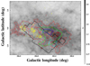Fig. 3.

Av extinction map (Dobashi et al. 2013). The red isocontours are A_Ks of 0.65, 1.55, 2.44, and 3.34 mag, respectively. The blue, green, and cyan contours underline extinction features at 2, 5, and 9.5 kpc respectively, delineated from Marshall et al. (2006) extinction data cubes. The Hα mosaic contour is drawn in black and the Hα emission of the main H II regions is displayed (from the larger-scale SuperCOSMOS Hα Survey (SHS) image) as yellow isocontours.

To estimate the velocity range for the extinction, we look at the discrete continuum sources for which Brown et al. (2014) probed the HI absorption along the source line of sight by applying the emission/absorption (E/A) method to HI spectra. Four sources between l = 281.5° and l = 285.5° show significant extinction features. The source G282.03–1.18 (v_LSR = +19 km s⁻¹, d_kin = 6.32 kpc) shows a large dip from ∼−20 to +25 km s⁻¹; G284.72+0.31 (v_LSR = +10 km s⁻¹, d_kin = 6 kpc) shows dips from ∼−20 to +20 km s⁻¹; while RCW 49 (v_LSR = +0 km s⁻¹, d_kin = 4.8 kpc) and G285.25–0.05 (v_LSR = −2 km s⁻¹, d_kin = 4.9 kpc) show a large dip from ∼−20 to +10 km s⁻¹. These results underline velocities in agreement with the velocity of the observed diffuse Hα layers and allow us to suppose that the different layers are forward and closer than ∼6.3 kpc.

3.2. H II regions kinematics and distance

In this section, we discuss the kinematics and distance determination of the individual H II regions (among which the two most remarkable are RCW 48 and RCW 49) present in the mosaic area (l = 280.8° to 285.5° and b = −2.3° to −1.1°).

Because the long path length through the arm lies in a narrow range of longitudes near the tangent, implying a heavy blending of the emissions, it is difficult to identify individual clouds or cloud complexes. However, from the HIPASS image (Calabretta et al. 2014), and assigning radio recombination line velocity from Caswell & Haynes (1987) and Wilson et al. (1970), we can identify the following six main radio continuum emission complexes: (1) l, b = 285.25°, −0.05°, V_LSR ∼ −2 km s⁻¹ (d_kin ∼ 4.8 ± 1.5 kpc); (2) l, b = 284.30°, −0.31° (clearly related to RCW 49), V_LSR ∼ −0.7 km s⁻¹ (d_kin ∼ 4.7 ± 1.5 kpc); (3) l, b = 283.87°, −0.86°, V_LSR ∼ +3 km s⁻¹ (d_kin ∼ 5.1 ± 1.3 kpc) showing extended emission to the west (where RCW 48 is located) and to the north; (4) l, b = 282.03°, −1.16°, V_LSR ∼ +19 km s⁻¹ (d_kin ∼ 6.3 ± 1.0 kpc) showing extended emission to the east; (5) l, b = 282.3°, −1.84°, V_LSR ∼ −15 km s⁻¹ (d_tan ∼ 1.8 kpc); and (6) l, b = 281.0°, −1.55°, V_LSR ∼ −5 km s⁻¹ (d_kin ∼ 3.2 ± 1.5 kpc). Between the third and the fourth structures (around l = 282.9°), the radio continuum emission shows a clear dip. This dip is also observed at infrared emission from 22/24 microns (MSX, WISE) to 100/140/160 microns (IRIS, AKARI). At higher resolution (e.g., at Spitzer 8 μm and Herschel-Hi-GAL 70 μm/160 μm), the dip is bordered to the west by bright rims and pillars (with typical velocity around −5 km s⁻¹, from Mège et al. 2021), and corresponds to strong absorption in Hα and optical images. In addition, from the low-resolution (7.5′) CO survey, Grabelsky et al. (1988) identified seven molecular clouds with velocities between −19 and +17 km s⁻¹ while, in the same area, Caswell & Haynes (1987, with a beam size of about 4.2′) identified 18 radio H II regions with velocity in the same range, between −15 and +19 km s⁻¹. Among these, 8 have no clear Hα counterpart, suggesting that they are either embedded young H II regions or extincted H II regions due to line-of-sight extinction. We note that they are all in Hα-dark areas, and are therefore strongly affected by line-of-sight extinction. For these regions, we mainly compare the WISE 22 μm, Spitzer 8 μm and/or WISE 12 μm (tracing the photodissociation region (PDR) expected to surround H II regions), and SUMMS (843 MHz) radio continuum emission (Bock et al. 1999) to evaluate their nature and evolutionary status. In the following subsections, we discuss the kinematics and distance of the H II regions.

3.2.1. Radio H II regions

G281.595–0.969 (V_LSR = +2 ± 1–−3.4 ± 0.1 km s⁻¹, d_kin= 4.1 ± 0.8 kpc, Fig. B.1) is a compact source in radio, 22 μm, and 8 μm emission, favoring a young and embedded H II region stage (in any case, out of our field it shows no Hα counterpart on the SuperCOSMOS Hα Survey⁴ (SHS) image), but its radio spectral index of 0.2 (from flux densities at 5 GHz and 843 MHz from Caswell & Haynes 1987 and Murphy et al. 2007 respectively) suggests it is a classical H II region. It can be associated to the sources AGAL G281.586-00.972 (Urquhart et al. 2014) and HIGALBM 281.5851-0.9716 (Elia et al. 2021; Mège et al. 2021), of which the assigned V_LSR is −2.1 km s⁻¹ and +2.6 km s⁻¹ respectively. It is difficult to physically interpret the two distinct velocities observed in radio recombination lines and molecular lines. However, the small variation of the distance according to the chosen velocity (from 3.7 to 4.5 kpc) allows us to adopt the mean distance (d_kin = 4.1 ± 0.8 kpc) for this region.

G282.026–1.180 (V_LSR = +20.5 ± 1.5 km s⁻¹, d_kin = 6.5 ± 0.2 kpc, Fig. B.2) is a compact radio source in an elongated radio continuum emission and is located in an extinction zone at the northern edge of RCW 46. The elongated emission is resolved as a collection of filamentary structures in the near- and mid-infrared images (as seen on Spitzer 8 μm/ WISE 12 μm and Hi-GAL 70 μm images). The radio source itself has a strong counterpart with a circular morphology in near- and far-infrared images (e.g., Spitzer 8 μm and Hi-GAL 70 and 500 μm) from which a size of ∼1.6′ can be estimated. With an estimated diameter of 3 pc, it is a typical H II region. Its velocity difference with RCW 46 suggests it is farther on the line of sight.

G282.240–1.099 (V_LSR = − 2 ± 1 km s⁻¹, d_kin = 4.0 ± 0.2 kpc, Fig. B.3) is a faint and extended emission on SUMMS with no clear counterpart at WISE 22 μm. It seems to be surrounded by a faint PDR as seen on WISE 12 μm and Hi-GAL 70 μm images. We therefore suspect that this is not really a H II region but is more likely part of a larger region. It is located at the edge of RCW 46, but due to their quite different velocity, their association is not obvious.

G282.260–1.810 (V_LSR = −15 ± 2.5 km s⁻¹, d_tan = 1.8 kpc, Fig. B.4) is a faint, extended radio emission crossed by filamentary features seen at WISE 12 μm and Hi-GAL 70 μm. Several Hi-GAL clumps lie along the filaments, suggesting that they are perhaps triggered star formation in a relic of an evolved H II region or a complex of H II regions.

G282.632–0.853 (V_LSR = 0 ± 2.5 km s⁻¹, d_kin = 4.6 ± 0.4 kpc Fig. B.5). On the SUMMS image, this object appears to be part of an ionized filament-like feature but on the WISE 12 μm image only diffuse emission structured in rims is seen. At WISE 22 μm, a small bow-shock-like structure can be noted. The source size (25′×10′) reported by Caswell & Haynes (1987) compared to the Spitzer 8 μm image suggests that it is certainly part of a larger-scale ionization front.

G283.131–0.984 (V_LSR = −1 ± 2.5 km s⁻¹, d_kin = 4.4 ± 0.4 kpc, Fig. B.6) is a strong and compact WISE 22 μm emission, while it resembles the “tip of an elephant’s trunk” at Spitzer 8 μm, suggesting it could be a young H II region triggered by a larger region. From Mège et al. (2021), the three closest Hi-GAL clumps have velocities of between −2.3 and −5.5 km s⁻¹, which is in agreement with the radio recombination line and the small surrounding Hα enhancement measured at −2.9 km s⁻¹.

G283.312–0.566 (V_LSR = +6 ± 2.5 km s⁻¹, d_kin = 5.3 ± 0.3 kpc, Fig. B.7). In the SUMMS image, this source belongs to an extended and filamentary feature. In the WISE 22 μm image, it is resolved into several sources, to which Hi-GAL clumps with similar velocity can be assigned; namely V_LSR = 5.78 kms⁻¹. No clear PDR is drawn on the WISE 12 μm image, and therefore the nature of the region is difficult to establish.

G283.329–1.050 (V_LSR = +16 ± 1 km s⁻¹, d_kin = 6.3 ± 0.1 kpc, Fig. B.8) is centrally strong and compact on the WISE 22 μm image and the morphology of the radio emission follows the features seen in the WISE 22 μm image relatively closely; these features are resolved into filaments in the WISE 12 μm and Hi-GAL 70 μm images. These surrounding filaments are thin and not very bright, suggesting that, if they trace the PDR, this latter is already strongly disrupted and therefore the H II region is evolved.

G283.978–0.92 (V_LSR = +3 ± 2.5 km s⁻¹, d_kin = 5.1 ± 0.3 kpc, Fig. B.9). The radio size of G283.978–0.92 reported by Caswell & Haynes (1987) is 20′×18′ and includes the more resolved radio sources listed in Table 1, such as G283.978–0.92 itself (which can be identified as G284.0–0.9 in Wilson et al. 1970 and G383.977–0.898 in Kuchar & Clark 1997), G283.832–0.730 (Wenger et al. 2021), and G284.014–0.857 (Wenger et al. 2021). G283.978–0.92 exhibits an elongated arc-like structure with no clear Spitzer 8 μm counterpart. Because it is better seen at Spitzer 4.5 μm and Hi-GAL 70 μm, this suggests that it is an ionization-dominated feature, which can delineate the inner edge of a bubble. G284.014–0.857 (V_LSR = +8.6 ± 0.1 km s⁻¹, d_kin = 5.7 ± 0.2 kpc) is a strong and compact (∼1.4′) WISE 22 μm and radio emission corresponding to the source IRAS 10184–5748, which was classified by Bronfman et al. (1996) as a compact H II region (with a CS velocity of +8.9 km s⁻¹, in agreement with the radio recombination line velocity). G283.832–0.730 (V_LSR = +6.3 ± 0.3 km s⁻¹, d_kin = 5.4 ± 0.03 kpc) is a strong and roundish WISE 22 μm and radio emission, but does not stand out from the background in Spitzer 8 μm and Hi-GAL 70 μm images. We therefore suppose that G283.832–0.730 is a more evolved H II region. However, G284.014–0.857 and G283.832–0.730 are on the eastern edge (labeled Rim 3 in Fig. B.9) of the infrared bubble E124 identified by Hanaoka et al. (2019) and identified by Zhu et al. (2009) to be a ring-like structure around the cluster [DBS2003] 45 (in the following, [DBS2003] refers to Dutra et al. 2003). In the Hi-GAL 70 μm image, the bubble can be delineated by three rims (labeled Rim 1 to 3 in Fig. B.9) along which several HI-GAL clumps are distributed. From the velocity of these clumps (Mège et al. 2021), one can assign a mean velocity of +14.6, +2.4, and +9 km s⁻¹ to Rims 1, 2, and 3, respectively. Rim 1 is the only one to have a radio continuum counterpart, suggesting it draws the edge of an ionized region. If we assume that G283.978–0.92, G283.832–0.730, G284.014–0.857, and the rims trace the same bubble, we can identify the far side (+14.6 km s⁻¹) and G283.978–0.92 as Rim 1, and the near side (+2.4 km s⁻¹) as Rim 2. This suggests that this bubble has a systemic velocity of ∼+8.5 km s⁻¹ (and an expansion velocity of about 6 km s⁻¹), which in agreement with the Rim 3 and G284.014–0.857 velocities. Zhu et al. (2009) postulated that the Hα emission seen is the ionized gas from this bubble, but the Hα emission velocity we measure and its extension (which is beyond the limits of this IR bubble) suggest it is not related. Indeed, in Hα, in the direction of this region, the Hα profiles decomposition shows a strong component with a velocity of around −5 km s⁻¹ and a second (faint) component with a velocity of around +10 km s⁻¹. The first component corresponds to a collection of emission enhancements and is related to the larger-scale foreground emission layer, while the second component has a velocity in agreement with the bubble systemic velocity, suggesting that some part of the Hα emission indeed comes from the bubble. The kinematic distances of the radio sources give a distance of 5.4 kpc for the bubble, which is initially different from the cluster [DBS2003]45 distance of 3.49 kpc given by Kharchenko et al. (2013). However, Mohr-Smith et al. (2017) recently identified seven OB star candidates in [DBS2003] 45 for which we estimated a mean $d_{Gaia} = 5 . 4_{- 0.79}^{+ 0.96}$ $d_{Gaia} = 5.4 ^{+0.96}_{-0.79}$ kpc, in agreement with the kinematic distance and confirming the link between [DBS2003] 45 and the bubble.

Table 1.

Radio sources and H II region information.

3.2.2. Optical (Hα) H II regions

GUM 30 (BBW 316C) is a very bright H II region located at the eastern edge of our mapped area. Its Hα systemic velocity is −19 km s⁻¹ and there is no noticeable velocity gradient. Because its velocity is forbidden, its kinematic distance cannot be calculated. However, GUM 30 is excited by the cluster NGC 3293, for which the most recent Gaia EDR3 distance is 2.35 ± 0.05 kpc (Göppl & Preibisch 2022), in agreement with the previous values of 2.33 ± 0.05 kpc (Dias et al. 2021) and 2.477 ± 0.017 kpc (Cantat-Gaudin et al. 2018). One can note that GUM 30 presents a velocity difference with the tangent point of only 5.4 km s⁻¹ (the distance and velocity of the tangent point on the line of sight of GUM 30 are 2.3 kpc and −13.6 km s⁻¹ respectively), which is of the order of the typical value of the cloud–cloud velocity dispersion in the Galaxy (between 3 and 8 km s⁻¹, e.g., Clemens 1985; Stark & Brand 1989; Stark & Lee 2006). This means that we could reliably adopt the tangent point distance (d_tan = 2.3 kpc) for GUM 30, which is in good agreement with the distance of the exciting cluster.

G285.253–0.053. In Fig. B.10, this region is a small Hα region (size ∼1.6 × 0.8 arcmin) very close to the bright H II region G30, but despite its apparent proximity, it has a very different velocity (Hα mean velocity = −9.5 km s⁻¹). Its quite different radio H109α velocity of −2 km s⁻¹ (Caswell & Haynes 1987) could be understood as being due to internal motion, as its Hα line exhibits a large width (FWHM = 32.5 km s⁻¹). G285.253–0.053 also appears to be the optical counterpart of the source HIGALBM285.2521–0.0343 for which Mège et al. (2021) give a CO molecular line velocity of +3.77 km s⁻¹. Performing the profile decomposition with two components instead of one, we find them at +3.2 and −13.8 km s⁻¹. In this way, the first component has the same velocity as the CO, while the second component can be interpreted as an ionized gas flowing toward us. We therefore favor a systemic velocity of +3.77 km s⁻¹ leading to d_kin = 4.7 kpc.

RCW49 and its surroundings. RCW 49 is mainly excited by the well-studied young (< 2 Myr, Zeidler et al. 2015) cluster Westerlund 2 (e.g., Carraro & Munari 2004). Westerlund 2 (Wd2) contains a dozen early O stars and two WR stars and seems to be split into two substructures: the main cluster of Wd2 and a smaller stellar group 45″ to the north (Zeidler et al. 2015). Its distance was estimated to be between 2.2 kpc and 8 kpc (e.g., Brand & Blitz 1993; Ascenso et al. 2007; Rauw et al. 2007; Hur et al. 2015). One of the most recent distance estimations is 4.207 ± 0.133 kpc, which was derived by Cantat-Gaudin et al. (2018) from Gaia-DR2 data.

Regarding distance, the radio recombination line systemic velocity of RCW 49 was not well constrained, as velocities of around 0 km s⁻¹ (d_kin = 4.8 kpc) and 9.8 km s⁻¹ (d_kin = 5.9 kpc) have been measured (Benaglia et al. 2005, 2013; Caswell & Haynes 1987; Paladini et al. 2015). Zeidler et al. (2021) recently measured a median radial gas velocity of 15.9 km s⁻¹, which translates to an LSR velocity of −1 km s⁻¹.

Radio continuum and mid-infrared observations reveal two wind-blown shells in the core of RCW 49 (e.g., Churchwell et al. 2004; Whiteoak & Uchida 1997) surrounding the cluster Wd2 (containing the binary star WR 20a) and the star WR 20b, respectively. The shell surrounding Wd2 has an outer diameter of 7.3′ and is opened as a blister structure on its western side. The shell surrounding WR 20b has an outer diameter of 4.1′ and the contact zone between the two shells delineates a ridge, which is the brightest source of emission at both radio and IR wavelengths (e.g., Paladini et al. 2015) but also in Hα (Fig. 4). More recently, Tiwari et al. (2021) delineated the global shell surrounding RCW 49 in [C II], finding velocities of between −12 and 0 km s⁻¹. This shell has a well-defined eastern arc, while the western side is blown open and is venting plasma further toward the west.

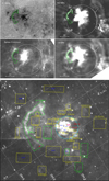Fig. 4.

Significant structures and velocities of RCW 49. Upper panel: mutliwavelength views of RCW 49. The white arrows point to Hα patches with positive velocity and the green contour delineates the arc-like feature. The white dashed circle underlines the circular radio emission feature. Lower panel: velocity (in km s⁻¹) of the different components (sorted by decreasing peak intensities) of the Hα profiles averaged over the areas shown. Coordinates are Galactic (in degrees). Zones dominated by negative (positive) velocity are shown in yellow (green). Values in red have similar intensities while values in blue indicate profiles fitted with a single component. The symbol “ ” indicates that the component has a FWHM ≥ 35 km s⁻¹. The magenta, black, and red stars indicate the positions of Wd2, WR21a, and Collinder 220, respectively.

From the CO transition, molecular clouds at −4, +4, and +16 km s⁻¹ are detected (e.g., Dame 2007; Furukawa et al. 2009; Ohama et al. 2010) in the direction of RCW49. Ohama et al. (2010) underline that the −4 km s⁻¹ and +4 km s⁻¹ clouds do not form distinct entities and that the spectra in the −11 to 9 km s⁻¹ range are sometimes complex and blended. The +16 km s⁻¹ and +4 km s⁻¹ clouds are found behind and in front of RCW 49, respectively (Dame 2007; Furukawa et al. 2009; Ohama et al. 2010), but heated by Wd2 (Ohama et al. 2010). The +16 km s⁻¹ cloud matches the ridge and extends beyond the nebula, while the 4 km s⁻¹ cloud is a good match to the IR nebula (Ohama et al. 2010). In summary, Furukawa et al. (2009) identified two molecular clouds at 4 km s⁻¹ and 16 km s⁻¹ and Furukawa et al. (2009) and Ohama et al. (2010) argued that their collision (∼4 Myr ago) is responsible for triggering the formation of Wd2. Tiwari et al. (2021) constrain the kinematics of RCW 49, showing three main structures: the expanding shell in the velocity range of −12 to 0 km s⁻¹, the northern and southern clouds in the velocity range of 2–12 km s⁻¹, and the ridge in the velocity range of +16 to +22 km s⁻¹.

Figure 4 compares the Hα emission to the radio continuum (at 843 MHz, Bock et al. 1999 and 1.4 GHz, McClure-Griffiths et al. 2005) and Spitzer 8 μm emissions. Churchwell et al. (2004) underline that Spitzer images of RCW 49 reveal a complex nebular structure with filaments, knots, pillars, and bow shocks. However, most of these features are not seen in absorption on the Hα image but are anyway located in smooth absorbed areas. This could suggest that the RCW 49 region is opened to the front, with the dust features mainly located at the rear. In Hα, toward the center of the Wd2 shell, we note double-peaked profiles (Figs. 4 and 5), suggesting an expansion velocity of 20 km s⁻¹ (in agreement with Tiwari et al. 2021). Similarly to the molecular profiles, the Hα profiles are complex. Toward the ridge, the profiles are very broad (FWHM between 40 and 60 km s⁻¹) and with velocities of between −6.4 and +3.0 km s⁻¹, while toward the external patches, the multicomponent decomposition of the profiles can be explained by blue and/or red wings around a main component underlining higher (absolute) velocity and complex kinematics (Fig. 5). Such wings around a main component are observed in extragalactic H II regions (e.g., Rozas et al. 2006; Relaño & Beckman 2005) as well as in supernova remnants (SNR; e.g., Sánchez-Cruces et al. 2018; Rosado et al. 2021); in such profiles, the main emission component is attributed to the bulk of the H II region, while the wings are attributed to the expanding shell. The mean Hα velocity of the ridge and the external patches is −5.4 km s⁻¹, in agreement with the velocity range of the expanding shell measured by Tiwari et al. (2021). Adopting this velocity as the systemic velocity, we can derive a kinematic distance of 4.1 kpc, which agrees with the most recent stellar distance estimation of 4.207 ± 0.133 kpc derived by Cantat-Gaudin et al. (2018) from Gaia-DR2 data.

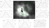Fig. 5.

Representative Hα profiles from the central part of RCW 49 are shown all around the displayed Hα image. The Hα profiles are extracted from the areas delineated on the image. The axes are the V_LSR in km s⁻¹ (X axis) and intensity in arbitrary units (Y axis). The profiles are decomposed into one to three components (labeled from 0 to 2). The solid and dash dotted lines are the observed and the fitted profiles, respectively. All profiles were observed with the P = 2604 interferometer.

In addition to RCW 49 itself, we note an arc-like feature (about 17′ to the east) and two Hα patches (to the west) with positive velocity (+12 and +8.1 km s⁻¹ respectively; Fig. 2) delineating a possible shell of ∼24.2′ in radius and centered at l,b ∼ 284.27°, −0.44° (see Fig. 4). We can assign a Hα mean velocity of ∼+10 km s⁻¹ to this shell. The mean velocity of the arc is +6.1 km s ⁻¹, which is in agreement with the +9 km s⁻¹ of the radio source G284.559–0.183 (Caswell & Haynes 1987) located on the southern part of the arc. G284.559–0.183 appears relatively compact at WISE 12 μm and appears, from the Spitzer 8 μm image, to be the heated tip of a PDR. The morphology of the arc-like feature on Spitzer 8 μm (tracing the PDR) suggests that it delineates a PDR heated on its eastern side. The Hα emission between RCW 49 and the arc is very patchy, with velocities mainly around −11.6 km s⁻¹ (Fig. 4) and profiles with a strong red wing, suggesting a flow. In addition, at the position α, δ = 10h25m49.3s, −57°39′55.2″, the profile is double peaked (with velocities around −11.8 and 25.1 km s⁻¹), suggesting a local expansion of about 18.5 km s⁻¹ around a systemic velocity of ∼6.7 km s⁻¹. The kinematics does not allow us to come to conclusions as to the link between the arc-like feature, its inner emission, and RCW 49. Belloni & Mereghetti (1994) show that the extended X-ray emission from RCW 49 is well correlated with the optical emission (and explained by a wind-blown bubble), while toward the inner part of the arc-like feature, the X-ray emission is softer and anti-correlated with the optical emission (and an SNR or wind-blown bubble might explain this emission). Belloni & Mereghetti (1994) suggest that the source of the X-ray emission at the origin of the arc could be either the Wolf-Rayet star WR21a or the cluster Collinder 220. Indeed, because the measured velocities are typical of H II regions or wind-blown bubbles, an SNR can be excluded as the origin of the X-ray emission. In the H II region, the diffuse X-ray emission is attributed to shocked stellar winds (e.g., Dunne et al. 2003; Townsley et al. 2003). Kinematically, unless the ambient density is high, the photodissociation dominates the region dynamics in the H II region compared to the stellar wind bubble (Capriotti & Kozminski 2001). However, on the other hand, most of the main sequence stellar wind bubbles in the H II region have expansion velocities of 10–20 km s⁻¹ (Nazé et al. 2001). Nevertheless, the position of Collinder 220 is shifted with respect to the arc-like feature and its inner emission, and its distance of 2.2 kpc (see Table A.1 for reference) places it in front of RCW 49, suggesting it is probably not the exciting source.

RCW48 is a ring nebula associated with the Wolf-Rayet star WR18 (e.g., Chu et al. 1983; Toalá et al. 2017), with an expansion velocity of around 15 km s⁻¹ (Chu 1988; Marston 2001). Hamann et al. (2019) give a distance of 3.9 $_{- 0.5}^{+ 0.8}$ $^{+0.8}_{-0.5}$ kpc (from Gaia-DR2) for WR 18, which is the distance we adopt for RCW48. The nebula has an elongated shape (18′ × 22′ in size), with its central star off-centered toward the west (located near the bright nebular arc), and a complex structure of radially distributed filaments pointing outward from WR 18 (Toalá et al. 2017). Toalá et al. (2017) suggest that these features most likely result from shadowing instabilities (e.g., Williams 1999; Arthur & Hoare 2006): the dense western arc fragments into dense clumps and the UV flux from WR 18 passes through gaps between clumps to produce the radial features. Given that Toalá et al. (2017) show that WR18 is not a runaway star (and its motion does not point toward the arc), the shape of the bright arced nebula cannot be a snow-plough shock. Arthur (2007) suggests that this morphology could be due to the environment, as the region is bounded on the arc side by molecular clouds (Marston 2001). Based on an analysis of X-ray properties, Toalá et al. (2017) revealed temperature and abundance variations within the nebula. These authors show that the regions close to the optical arc are hotter and that the abundances enhanced therein, suggesting heating and enrichment by the stellar wind from WR 18; while to the east, the gas exhibits abundances close to those reported from optical studies of the nebula, suggesting a mixing of the nebular material with the stellar wind.

In Hα, we observe a velocity gradient across the nebula (Fig. 6) and broad and asymmetric profiles (Fig. 7) underlining complex kinematics. This gradient was already highlighted by Deharveng & Maucherat (1974) and interpreted as a general nebular expansion at about 30 km s⁻¹, with positive velocities near the star and with the velocity becoming progressively more negative toward the bright arc. These latter authors also noted evidence for a very broad (∼80 km s⁻¹) line. Chu (1982) also noted the velocity gradient and observed line splitting, which extended from about 3′ west to about 14′ east of WR18, and derived an expansion velocity of 18 km s⁻¹. This gradient and the expansion can explain the difference between the radio recombination line velocity (V_LSR = +3 km s⁻¹, Caswell & Haynes 1987) and the mean Hα velocity of −7.2 km s⁻¹ that we measure. Adopting this last velocity as the systemic velocity gives d_kin = 3.6 kpc, which is in agreement with the distance of WR18. Marston (2001) observed that CO gas is not seen within the optically bright arc but adjacent to it, with strong line components at −16 km s⁻¹ and +9 km s⁻¹ to the north and at +7 km s⁻¹ to the south. Toward WR18, these authors show two main CO components at −5.5 km s⁻¹ and +4.6 km s⁻¹, respectively, in agreement with the main component velocities that we observe in Hα around the star.

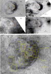Fig. 6.

Significant structures and velocities of RCW 48. Upper panels: SHS Hα (A), radio continuum SUMSS (843 MHz) (B), Spitzer 8 μm (C), and WISE 22 μm (D) images of RCW 48. Lower panel: Velocity (in km s⁻¹) of the different components (sorted by decreasing peak intensities) of the Hα profiles averaged over the areas shown in the Hα image. The blue arrow is the tangential velocity vector of the star WR18. The red and blue circles delineate the small and large shells discussed in the text, respectively.

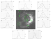Fig. 7.

Representative Hα profiles from RCW 48 are shown all around the displayed Hα image. The Hα profiles are extracted from the areas delineated on the image. The axes are the V_LSR in km s⁻¹ (X axis) and intensity in arbitrary units (Y axis). The profiles are decomposed into one to three components (labeled “0” to “2”) and night sky lines (labeled “N”), when necessary. The solid and dash dotted lines are the observed and the fitted profiles, respectively. All profiles, except (7) and (8), were observed with the P = 796 interferometer.

Combining multiwavelength images, two shells can be distinguished in Fig. 6. This is not surprising as multiple concentric shells are commonly observed around WR stars (Marston 1996). The larger shell of ∼9.4′ (∼10.7 pc) in radius and centered at l, b = 283.64°, −0.94° is mainly delineated from Hα emission and has a mean velocity of −8.6 km s⁻¹. The smaller shell with a radius of 3.8′ (∼4.3 pc) is centered on WR18 and is mainly delineated following the radio and WISE-22 μm arc curvature. Despite the fact that the WISE-22 μm emission is quite weak and patchy, the arc clearly traces the stellar wind bubble, as Mackey et al. (2016) show that the outer edge of a wind bubble emits brightly at 24 μm through starlight absorbed by dust grains and reradiates thermally in the infrared. No strong PDR is detected at Spitzer-8 μm; however, at the position of the optical bright arc, 8 μm rims are noted pointing toward WR 18 (Fig. 6C), confirming the link between the star and the arc. Inside the eastern part of the larger shell, the rims point in the opposite direction of WR 18 and toward the infrared bubble E124 (Hanaoka et al. 2019), which is farther along the line of sight.

The asymmetry of the profiles necessitates their decomposition into two or three Gaussian components (Fig. 7), which can be interpreted as a main component with blue and/or red wings. This is the signature of an expanding shell. In some directions pointing toward the center of the large shell, the wing velocity reaches −86.5 km s⁻¹ and/or +38.7 kms s⁻¹ for the blue and red component, respectively, suggesting strong internal motions. One profile shows a clear splitting with the two components separated by 41.5 km s⁻¹, from which an expansion velocity of 20.8 km s⁻¹ can be estimated. Toward the arc, the profiles show strong asymmetry with a main component and a blueshifted component with mean velocities of −5.7 and −48.8 km s⁻¹, respectively. Our findings for the Hα kinematics are in agreement with the expected scenario for the WR nebula (e.g., van Marle et al. 2015; Georgy et al. 2013), which is that the wind from the WR star sweeps up and compresses the previously ejected material into a shell, while the UV flux ionizes the material. In this frame, the large shell is probably the signature of any previous mass-loss episodes, while the arc underlines its interaction with the actual WR 18 stellar wind bubble.

G281.013–1.528 and G281.162–1.640. These two regions (Fig. B.11) have Hα velocities (v_LSR = −5 and −6 km s⁻¹ for G281.013–1.528 and G281.162-1.640 respectively) that are in agreement with that derived from radio observations by Caswell & Haynes (1987). In the Hi-GAL 70 μm image, they belong to a ∼19.3 arcmin elongated star-forming region in which several molecular clumps with similar velocities (from −9 to −6 km s⁻¹) have been identified (clumps BYF 4–8 from Barnes et al. 2011). On a higher-resolution SHS Hα image, G281.013-1.528 appears extended (∼7′ × 9′) with dust lanes crossing it, while G281.162–1.640 is compact (size ∼1.6′). This suggests that G281.013–1.528 is more evolved than G281.162–1.640. Indeed, G281.162–1.640 is classified as an UCH II region (Bronfman et al. 1996) and has a CS(2–1) velocity of −6.2 km s⁻¹. In addition, an infrared open cluster is identified toward G281.162-1.640 ([DSB20003]125, Dutra et al. 2003) with an evaluated distance of 2817 pc (Kharchenko et al. 2013), which is in agreement with the kinematic distances of 3.2 kpc and 3.1 kpc for G281.013-1.528 and G281.162-1.640, respectively.

RCW46, G282.24–1.099, and G282.0–1.18. RCW 46 is a ∼25′ large H II region (Figs. 1 and B.12) centered at l, b = 282.32°, −1.29°. In the literature, it is often misidentified as the compact (∼3′) radio H II region G282.03–1.18 (Caswell & Haynes 1987), which has a radio recombination line velocity of around +20 km s⁻¹ (Wilson et al. 1970; Caswell & Haynes 1987) and is excited by the NIR cluster (for which Moisés et al. 2011 estimate a distance of 6.97 kpc). The optical H II region RCW 46 has a mean velocity of −11 km s⁻¹ with a possible gradient from the border to the center of about 4–7 km s⁻¹. Near the center of RCW 46, several sources can be found: IRAS 10058-5718, toward which four Hi-GAL sources (Elia et al. 2021) are identified with a velocity of −15 km s⁻¹ (Mège et al. 2021); the BRAN 288 region, with a molecular velocity of −18 km s⁻¹ (Brand & Blitz 1993); and the NIR cluster DBS42 (Dutra et al. 2003), within which Soares et al. (2008) find the brightest star to be only an A8-9 IV (Av = 1.35). Because these velocities are forbidden, the kinematic distance cannot be calculated for these objects. At about 6.5′ from the center, there are two possible hot stars: HD 302532 (B3; Nesterov et al. 1995) and CPD-56 2853 (B1; Loden et al. 1976) with d_Gaia = 2.4 and 2.25 kpc, respectively. We note that, on the west border, there is the NIR cluster MWSC1765; but with an estimated distance of 9.5 kpc (Buckner & Froebrich 2013), it cannot be related to RCW 46. The northern part of RCW 46 spatially overlaps G282.24–1.099, which is a large (12′ diameter) radio continuum source listed by Caswell & Haynes (1987) at −2 km s⁻¹, suggesting that RCW 46 could be its optical extension. For G282.24–1.099, d_kin is 4 kpc, which is in good agreement with d_Gaia = 4.45 kpc (Cantat-Gaudin et al. 2018) of the open cluster MWSC 1774 (Kharchenko et al. 2012) noted in its direction. We favor this last explanation and then adopt this last distance for RCW 46.

BRAN 293 is a ∼10.7′ × 5′ enhancement in Hα, with a velocity of −6 km s⁻¹. The molecular velocity attributed by Brand et al. (1987) is −15.3 km s⁻¹, but on the east edge of the feature is the clump HIGALBM282.8392-1.2434 (Elia et al. 2021), which has v_LSR = −4.47 km s⁻¹ (Mège et al. 2021) and corresponds to the compact radio H II region G282.842–01.252 listed by Wenger et al. (2021) with a recombination line velocity of −4.2 km s⁻¹. Adopting −4.47 km s⁻¹ as the systemic velocity, this gives d_kin = 3.87 kpc. Furthermore, looking toward the south extinction area, a bluish emission can be noted on the DSS2 color image, suggesting that this object is a reflexion nebula, for which we estimate a velocity of about −19.4 km s⁻¹ (as this velocity component dominates in Hα), which is in better agreement with the molecular velocity given by Brand et al. (1987). In this frame, this reflexion nebula can be attributed at least to the stars HD 302584 (B1III, d_Gaia = 2.54 ± 0.09 kpc) and HD 302583 (B0V, d_Gaia = 2.54 ± 1.41 kpc) and this suggests that the −15.3 km s⁻¹ from Brand et al. (1987) corresponds to a foreground feature with a distance of around 2.5 kpc.

RCW47. This H II region (Fig. B.14), extending over 24′, is composed of two structures with velocities of between −3 and −5 km s⁻¹, while Brand & Blitz (1993) give a CO velocity of −17.6 km s⁻¹ (BRAN 285). Several dark extinction features are noted on the SHS Hα image, which can be related to the dark cloud 282.69-2.51 (Dutra & Bica 2002) toward which Otrupcek et al. (2000) measure CO velocities of −5 km s⁻¹ ( $T_{A}^{*} = 2.8$ $T^{*}_{A} = 2.8$ K, FWHM = 2.8 km s⁻¹) and −17.3 km s⁻¹ ( $T_{A}^{*} = 9$ $T^{*}_{A} = 9$ K, FWHM = 4.2 km s⁻¹). In parallel, RCW 47 can be associated to a molecular cloud (cloud number: 4666) identified by Miville-Deschênes et al. (2017) with a central velocity of −7.78 km s⁻¹. We therefore favor a velocity of −5 km s⁻¹ for RCW 47. Four massive stars are listed in the direction of RCW47: HD 302501 (O9III from Bigay et al. 1972, d_Gaia = 2.21 ± 0.11 kpc), LS1414 (B1V photometric, d_Gaia = 2.31 ± 0.07 kpc), HD 302505 (O9.5III from Bigay et al. 1972, d_Gaia = 2.37 ± 0.07 kpc), and HD 87643 (B3I[e]; Skiff 2014 $d_{Gaia} = 1 . 95_{- 0.48}^{+ 1.8}$ $d_{Gaia} = 1.95^{+1.8}_{-0.48}$ kpc). However, HD 87643 has a RUWE value of greater than 1.4 (RUWE = 9.82; Gaia Collaboration 2020), indicating that the source is nonsingle, or problematic for the astrometric solution. Discarding HD 87643, we can then adopt a mean distance of 2.29 kpc for RCW47.

H2 (BRAN 299) and G283.312–0.566. In Hα, BRAN 299 shows a bright part (coinciding with IRAS 10140-5707) and a more diffuse emission (Fig. B.15) located on the border of a strong extinction region behind which the radio source G283.312–0.566 is located. Caswell & Haynes (1987) give a radio recombination line velocity for G283.312–0.566 of +6 km s⁻¹ (d_kin = 5.3 kpc) and a size of 8′ × 10′, while in the direction of the source, Russeil & Castets (2004) measure a ¹³CO velocity of −7.3 km s⁻¹ and Miville-Deschênes et al. (2017) identify a ¹²CO cloud at +3.6 km s⁻¹ (cloud [MML2017] 2335). BRAN 299 could have been linked to the radio source G283.312–0.566, but given their velocity difference, we consider them to belong to two different clouds at −7.3 km s⁻¹ and +3.6 km s⁻¹, respectively. The BRAN 299 brightest part has an Hα velocity of −12 km s⁻¹ while the more diffuse part has a smaller velocity of −9.9 km s⁻¹. As the −12 km s⁻¹ is a forbidden velocity, preventing kinematic distance calculation, one can assign the tangent point distance (d_tan = 1.9 kpc), which has a very similar velocity (−11 km s⁻¹). BRAN 299 is also catalogued by Magakian (2003) as a reflection nebula illuminated by the B1Ia/ab star HD 89201 with d_Gaia = 2.20 ± 0.10 kpc, which is in agreement with the kinematic distance we adopt here.

RCW50. Well seen in Hα, RCW50 shows no clear radio or infrared counterpart (Fig. B.16), and therefore its nature is unclear. The Hα profile of this region can be fitted with either a broad (FWHM = 30 km s⁻¹) Gaussian at a velocity of −7 km s⁻¹ (Fig. 8-1) or two Gaussians (of FWHM = 22.5 km s⁻¹ each), either at velocities of −11 and +3.2 km s⁻¹ or at velocities of −3 and −17 km s⁻¹; in both cases, the first velocity component is about twice as intense (Figs. 8-1,2). This could suggest a flowing motion of the ionized gas. Located at the border of a large extinction area centered at (l, b = 283.78°, +0.21°), RCW50 overlaps with an extended AKARI 60 μm (not covered by the Hi-GAL survey) emission (size 12.8′×11.5′) located 6.8′ to the northwest. This latter 60 μm region could be associated with the radio continuum source G284.260+0.400 (Caswell & Haynes 1987), which is of a similar size (15’ × 9’) and has a radio line velocity of +1 km s⁻¹ (Caswell & Haynes 1987; d_kin = 4.9 kpc). However, the link between RCW 50 and G284.260+0.400 is not clear because of their spatial shift and velocity difference. Looking at molecular clouds delimitated by Miville-Deschênes et al. (2017), RCW 50 can be placed at the border of three clouds: 4867 (v_LSR = −1.75 km s⁻¹), 1830 (v_LSR = −7.11 km s⁻¹), and 4859 (v_LSR = −1.47 km s⁻¹). The cloud 1830 corresponds to GMC 7 in Grabelsky et al. (1988), and because of its high column density (1.93 × 10²¹ cm⁻²) with respect to the two other clouds (593 and 804.7 cm⁻²), it is the most probable star forming cloud. Furthermore, given its similar velocity to RCW50, it could be linked to it. With a velocity of −7 km s⁻¹, this leads to d_kin = 3.6 kpc (far distance choice). Only three OB star candidates are found toward RCW50 by Mohr-Smith et al. (2017), but these stars, identified as 1295, 1228, and 1271, have very different distances (d_Gaia = 2.21 ± 0.38 kpc, 3.36 ± 0.55 kpc, and 4.57 ± 0.64 kpc, respectively), preventing any reliable determination of the stellar distance for the region. We therefore adopt the kinematic distance for RCW50.

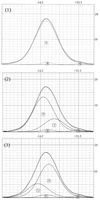Fig. 8.

Hα profile from RCW50. The profile can be decomposed in three ways (panels 1–3). The axes are the V_LSR in km s⁻¹ (X axis) and intensity in arbitrary units (Y axis). The profile, in addition to the night sky lines (labeled “N”), can be decomposed into either one component (panel 1) or two components (panels 2 and 3), labeled “0” and “1”. The solid and dash dotted lines are the observed and the fitted profiles, respectively.

G284.650–0.484 has in Hα an annular morphology (size ∼3.1′) that is clearly surrounded by a PDR (Fig. B.17). The PDR (also well seen on Hi-GAL 70 μm image) surrounds the ionized gas as traced by the radio continuum and Hα emission. The SUMSS image shows an intensity gradient from the southeast to the northwest, while the Hα emission displays a center-to-border intensity gradient. In Hα, the less intense central part has a velocity of −12 km s⁻¹, while the brighter border displays velocities of between −2 and −6 km s⁻¹, suggesting that it is a flow of matter toward us and seen from the front. The mean Hα velocity for the region is V_LSR = −4.7 km s⁻¹, which is different from the velocities derived from radio observations, of V_LSR = +5 km s⁻¹ (with a relatively narrow line width of 14 km s⁻¹; Caswell & Haynes 1987), and from molecular lines, namely V_LSR = +3 km s⁻¹ (from the associated Hi-GAL sources; Mège et al. 2021). From Mohr-Smith et al. (2017), two OB stars, #1550 (Gaia DR3 5255622016945421056) and #1557 (Gaia DR3 5255621845141987328), are found in the direction of the region. These stars have $d_{Gaia} = 3 . 19_{- 1.13}^{+ 2.19}$ $d_{Gaia} = 3.19^{+2.19}_{-1.13}$ kpc (but with RUWE = 10.366 and π/σ_π = 1.78) and $d_{Gaia} = 4 . 6_{- 0.93}^{+ 1.20}$ $d_{Gaia} = 4.6^{+1.20}_{-0.93}$ kpc (more reliable because RUWE = 0.913 but π/σ_π = 3.37). These stellar distances favor d_kin = 4.3 kpc (for V_LSR = −4.7 km s⁻¹) instead of d_kin = 5.2 kpc (for V_LSR = +3 km s⁻¹). In this frame, the region rather has a systemic velocity of −4.7 km s⁻¹ with the rear side at +5 km s⁻¹ and near side at −12 km s⁻¹ underlining an expansion velocity of about 8.5 km s⁻¹.

BRAN 302. In Hα (Fig. B.18), this region is small (∼3.7′ × 2.5′) and has a velocity of −6.4 km s⁻¹ (d_kin = 3.8 kpc, far distance). No radio, Hi-GAL 70 μm, or AKARI 60 μm counterparts are noted, meaning that the nature of this H II region is unclear. However, it can be associated to a WISE 22 μm emission. If it is a H II region, at the center of the nebula, the only possible exciting star would be the variable star HD 302686 (B3V/O9.5V; Reed 1998), for which d_Gaia = 2.34 ± 0.08 kpc, which is quite different from d_phot (between 2.6 and 4.1 kpc, depending on the photometric value set used as listed in Reed 1998) and d_kin = 3.8 kpc. We adopt d_Gaia.

G284.723+0.313, discovered by Bronfman et al. (1996), is observed in Hα (Fig. B.19) as a very small feature (size ∼48″) with a velocity of +14.2 km s⁻¹, which is in agreement with the velocities derived from molecular (+12 km s⁻¹; Bronfman et al. 1996) and radio recombination lines (+10 km s⁻¹; Caswell & Haynes 1987). The Hα comes from only a small part of the H II region as seen in radio and IR wavelengths, suggesting a strong extinction along the line of sight. No exciting star can be identified, and so we adopt the kinematic distance of d_kin = 6.2 kpc (for V_LSR = +12 km s⁻¹) for this region.

Table 1 summarizes the velocities and distances of the H II regions. Despite the difficulty in establishing a reliable distance, we note that the H II regions lie between 2.2 and 6.3 kpc. This distance range can be considered as an estimate of the thickness of the Carina arm along the tangent direction. We also note that several Hα regions (e.g., RCW 50 and RCW 46) do not follow the typical H II region structure with a radio/Hα emission more or less centered on an exciting source (OB star(s) or cluster) and surrounded by a PDR. These regions are also difficult to explain as light scattered off the interstellar dust grains, because they do not show the expected IR (around 100 μm) counterpart (e.g., Mattila et al. 2007).

4. Characterization of the Carina arm tangency

As discussed by Hou & Han (2014), the determination of the tangent direction to the Galactic spiral arms depends on the tracers (CO, HI, H II regions, old stars, etc.), the identification method (e.g., local maxima in a longitude plot of integrated emission, source counting, or arm fitting through the 2D distribution of Galactic plane tracers, etc.), and the uncertainties and dispersion (e.g., velocity crowding and streaming motions, optical depth effects, etc.). The Carina tangent direction is not delineated from near- or mid-infrared star (old stars) counting (Hou & Han 2015; Benjamin et al. 2005), suggesting it contains mainly gas visible as H II regions.

We first reinvestigated the Carina tangent direction by combining HI and CO longitude–velocity plots (Fig. 9). The emission shows a clear enhancement at l = 280°, which then clearly splits into the near and far parts of the Carina arm for longitudes of greater than 285°. The Carina arm is easily distinguishable from the other arms as traced by the faint emission features with velocities of higher than +40 km s⁻¹. The molecular velocities spread out between −11 and +7 km s⁻¹ at l ∼ 281.6° to −20 and +15 km s⁻¹ at l ∼ 286° while for longitudes between 273° and 279°, which are dominated by the local emission, velocities are between −3 and +5 km s⁻¹. The most significant H II regions (RCW 48, RCW 49, G30, and RCW 46) in our Hα line mosaic belong to the near part (negative velocities) of the Carina arm.

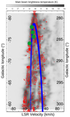Fig. 9.

Longitude–velocity plot of the CO emission from Dame et al. (2001; integrated over latitudes of between 0 and −1.2°) overplotted with HI emission from the HI4PI project (HI4PI Collaboration 2016). In blue, we show the plot of the Carina arm from the Hou & Han (2015) model. The green symbols show the position of the H II regions RCW 46, RCW 48, RCW 49, and G30 (ordered by increasing longitude).

We also investigated the Carina tangent from extinction in the Gaia G-band. Following Russeil et al. (2020), we produced ΔA_G-distance plots (Fig. 10). This is done by extracting the Gaia-DR2 data within a 1° radius area centered on the six positions along the Galactic plane (b = +0° and l = 280°, 281°, 282°, 283°, 284°, and 285°, respectively) and toward a reference direction (off position) pointing at l,b = 383°, +3°. We selected stars with π > 0, σ_π/π ≤ 0.2, and A_G > 0. We then calculated the error-weighted average and standard deviation of A_G in 0.05 mas parallax bins and calculating ΔA_G = A_G(region) −A_G(off position). From Fig. 10, we can follow the extinction variation along the Galactic plane. We note that the extinction starts to significantly increase at 1.8 kpc and that the maximum extinction is reached for l = 282°. This suggests that the tangent direction to the arm is located around l = 282°. Because this method is not reliable for distances beyond ∼2 kpc, we refrain from interpreting the relative positions of the peaks.

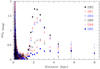Fig. 10.

A_G extinction versus distance plot for the six positions along the Galactic plane at l = 280°, 281°, 282°, 283°, 284°, and 285°, respectively.

To precisely decipher the line-of-sight extension of the tangency, we investigated the distribution of the young stellar population traced by the OB stars and the open clusters present in the region. Mohr-Smith et al. (2017) identified the OB stars in the longitude range 282° < l < 292.5° (and ∣b∣ < 2°), for which we re-estimate the distance by cross-matching (1″ cone search) them with Gaia-EDR3 (Gaia Collaboration 2020) and the Gaia-EDR3 distance catalog from Bailer-Jones et al. (2021). Selecting OB stars with RUWE ≤ 1.4 and π/σ_π > 5, we plot (Fig. 11) their distance distribution (limiting the sample to the longitude range from 282° to 285.5° overlapping our Hα mosaic). We highlight the narrow and broad peaks around 2.4 kpc and 4.5 kpc, respectively. The first peak can be interpreted as tracing the near edge of the arm, while the broad peak, in agreement with the RCW 48 and RCW 49 distance, can be interpreted as tracing the prominent part of the arm modulated by the lack of completeness at these higher distances. The Mohr-Smith et al. (2017) OB star sample distance distribution agrees with the Chen et al. (2019) and Xu et al. (2021) OB star samples and with the Zari et al. (2021) OBA star sample (Fig. 11).

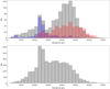Fig. 11.

Histograms of the Gaia distances of different samples. Upper panel: histogram of the Gaia distance of OB star candidates (between 282° and 285.5°) from Mohr-Smith et al. (2017; grey) overplotted with the Xu et al. (2021; blue) and Chen et al. (2019) OB stars samples (red). Lower panel: histogram of the Gaia distances of the OBA star sample from Zari et al. (2021). All stars follow RUWE ≤ 1.4 and π/σ_π > 5).

Table A.1 shows the open clusters and IR clusters and groups located between longitudes of 280° and 286° (and −2.5 < b < 0.5°) collected from literature. We note that clusters, similarly to the OB stars, also appear to form two distance layers at ∼2.4 kpc and 4 kpc. Three clusters are found at distances of between 6 and 6.6 kpc, with one of them being relatively young (FSR 1530), suggesting an upper limit for the arm of around 6.5 kpc, which is in agreement with the upper limit on the H II regions.

Combining with the distance range for the H II regions, one can conclude that the Carina arm tangent direction is located at l = 282° and that it stretches in distance from ∼1.8 kpc to ∼6.5 kpc in the longitude range probed here (between 281° and 285.5°), with an adopted mean distance of 4.5 ± 0.5 kpc (corresponding to a Galactocentric distance of 8.5 ± 0.3 kpc, for a Sun Galactocentric distance of 8.34 kpc) for the central part of the arm. This is illustrated in Fig. 12 by the pole-on view of the distributions of the H II regions and clusters.

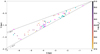Fig. 12.

Pole-on view of the distributions of H II regions and clusters. The full circles are the H II regions (color proportional to log(N_Lyc)), while the cyan and magenta squares are the young (log(age (Myr)) < 8) and old (log(age (Myr)) ≥ 8) clusters, respectively. The position of the Sun is x = 0 and y = 0.

5. Stellar kinematics at the Carina arm tangency

We take advantage of the Gaia proper-motion and parallax measurements to investigate the stellar kinematics, calculating the longitude (pmlong) and latitude (pmlat) proper motions. Two groups can be delineated when plotting (Fig. 13) the proper motions of the OB and OBA stellar samples. The most populated one (Group 1) is centered around pmlong, pmlat ∼ −6.29 mas yr⁻¹, −0.35 mas yr⁻¹, while the other one (Group 2) is around pmlong, pmlat = −7.97 mas yr⁻¹, −0.74 mas yr⁻¹. The proper motions converted (following Russeil et al. 2020) into the components of the transverse velocity in the Galactic region frame (named here Vlong and Vlat) give Vlong ∼ 1.09 km s⁻¹ and Vlat ∼ 0.3 km s⁻¹ for Group 1 and Vlong ∼ −16.5 km s⁻¹ and Vlat ∼ −1 km s⁻¹ for Group 2. As any peculiar motion in the Galactic disk in this frame will produce a shift with respect to the null value, only Group 2 appears to have a significant Vlong shift. In addition, we note that Group 1 (Group 2) consists mainly of stars at a mean distance of ∼4.2 kpc (∼2.6 kpc) and at negative (positive) latitudes. More precisely, from Fig. 14, we note that stars between 2.2 and 2.7 kpc show a Vlong distribution peaking at ∼−15 km s⁻¹ and ∼7.5 km s⁻¹ while no significant shift is observed for stars farther than 2.8 kpc. This can be interpreted by the fact that around 2.5 kpc, the stars are tracing both the trailing and the leading sides of the arm, while stars at greater distances better trace the inner part of the arm. The geometrical configuration of the line of sight with respect to the arm tangency means that Vlong is more representative of the Galactocentric radial velocity component, suggesting that stars with Vlong ∼ −15 km s⁻¹ (∼7.5 km s⁻¹) are moving outward (inward). This can be compared to simulated results from Kawata et al. (2014) who, despite the large dispersion found for the stellar Galactocentric radial velocities, show that the gas is moving outward (inward) in the trailing (leading) side of the spiral arm.

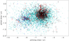Fig. 13.

Stellar proper motion for the following samples: Mohr-Smith et al. (2017; black), Xu et al. (2021; blue), Chen et al. (2019; red), and Zari et al. (2021; cyan), respectively.

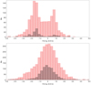Fig. 14.

Distribution of the stellar longitude velocity component (Vlong) of the Mohr-Smith et al. (2017; black) and Zari et al. (2021; red) stellar samples, respectively. The upper and lower panels show the distribution for stars with distances of between 2.2 and 2.7 kpc and farther than 2.8 kpc, respectively.

6. Star formation across the arm tangency

To investigate the star formation across the Carina arm tangent direction, we investigated the young stellar objects (YSOs), molecular clouds, and clumps distributions in the longitude range 280° < l < 286°. For the distribution of molecular clouds, we use the Milky Way molecular cloud catalog from Miville-Deschênes et al. (2017), while for the distribution of clumps we use the Hi-GAL catalog produced by Elia et al. (2021). These catalogs provide the velocity, distance (with the near/far distance ambiguity solved), and cloud or clump mass. Because we estimated that the arm tangency extends from ∼1.8 to 6.5 kpc, we also select only the clouds and clumps in this distance range. In addition, we evaluated the star-forming fraction (SFF) and the star formation rate (SFR) from the Hi-GAL catalog following Ragan et al. (2016) and Elia et al. (2022), respectively.

For the distribution of YSOs, we use the candidate YSO catalogs from Marton et al. (2019) and Kuhn et al. (2021). The former catalog provides an evaluation of the probability that a star is a YSO. We then selected the stars with a probability of being a YSO of higher than 90% and cross-matched them with Gaia-DR3 catalog (Gaia Collaboration 2020). We evaluated the YSO class (class I, II, III, or flat SED) from spectral index (calculated from the WISE magnitudes following Kang et al. 2017 using the boundaries from Greene et al. 1994). We then selected class I, II, and flat-spectrum YSOs within the parallax range 0.153 mas < π < 0.555 mas (allowing us to select stars with distances of between 1.8 and 6.5 kpc) and with RUWE ≤ 1.4 and π/σ_π > 5. In parallel, Kuhn et al. (2021) produced the Spitzer/IRAC candidate YSO (SPICY) catalog. In this catalog, the candidate YSOs were identified based on excess infrared emission consistent with the spectral energy distributions (SEDs) of pre-main sequence stars with disks or envelopes, using the YSOs analyzed by Povich et al. (2013) as templates. The authors then assigned a class (class I, II, III, or flat SED) to every star based on spectral index (using also the boundaries from Greene et al. 1994). Because the SPICY sample is significantly smaller (315 objects) than the Marton et al. (2019) sample, we do not apply any parallax selection.

Figure 15 shows the distribution of the YSOs, molecular clouds, and clumps versus the longitude. We have to keep in mind that when the longitude increases, we probe inter-arm to arm regions and that the direction of Galactic rotation goes from higher to lower longitudes. At longitudes of greater than 285°, the lines of sight cut both the near and far side of the Carina arm, superimposing the counting and therefore confusing the plots.

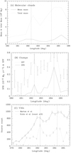Fig. 15.

Distribution of different star formation tracers. Distribution in longitude of: (A) the mean (black line) and the total mass (dashed line) per bin of the molecular clouds catalogued by Miville-Deschênes et al. (2017), (B) the SFF (dashed line) and the SFR (black line) calculated from the Hi-GAL catalog (Elia et al. 2021), and (C) the class I and II YSO counts extracted from the Marton et al. (2019; black line) and Kuhn et al. (2021; dashed line) catalogs, respectively.

All the plots agree in that they show an increase between 281° and 282°, confirming that the exit edge direction of the arm is in this longitude range. All the plots also display two peaks. Though clearly seen on the SFR plot around 282.3° and 284.3°, they appear less contrasted on the SFF and YSO count plots and at shifted positions (around 282.2° and 285.3° respectively) on the mean molecular cloud mass plot. Looking at the molecular cloud and clump catalogs, these are the sources at distances of around 5 kpc and 4 kpc (3.5 kpc for clumps), which mainly contribute to the highest peak and to the second-highest peak, respectively. For YSOs, the source number increase starts at 280°, while the mean YSO parallax from the Marton et al. (2019) sample is 0.339 mas (corresponding to a distance of approximately 2.9 kpc), suggesting that they allow us to only probe the outskirts of the arm.

The entrance edge of the arm can then be underlined by the highest molecular cloud mean mass peak at around 285.3°. Because the SFR peak at 284.3° corresponds to clumps at the same distance, we can interpret the shift as an evolutionary effect. Then, the angular shift Δl_{(CO − clumps)} = 1° translates into a linear distance of 78.8 ± 9 pc (for a distance of 4.5 ± 0.5 kpc). The second molecular cloud mean mass peak coincides with the second peak in the SFR plot. This position also corresponds to the H II region RCW 49 powered by the massive cluster Wd2 and located at a similar estimated distance, that is, of 4 kpc. The SFF, which is related to the evolutionary state of the clumps, follows the SFR but the variations are less clear. Assuming now that the main molecular cloud peak traces the arm entrance edge, and that the secondary peak traces the location of the main optical H II region (RCW 49), the angular distance Δl_{(CO − Hα)} = 3° can be translated into a linear width of 235.8 ± 26.2 pc.

Density wave theory predicts such a separation in space for different arm tracers, as Roberts (1969) suggested that star formation in spiral galaxies is triggered by a spiral density wave and predicted that Hα emission around newly formed stars should be offset and appear downstream from the gas spiral arm because of flow through the density wave. This induces an ordering of arm tracers along an “age gradient” across the width of a spiral arm. From measuring the offset between different tracers, and assuming that the pattern of a spiral arm is constant (angular pattern speed, Ω_p) and that the gas rotates in a circular orbit, we can infer the time it takes to go from the inner arm edge to the outer arm edge (e.g., Vallée 2020; Egusa et al. 2004; Louie et al. 2013). However, such offsets between molecular gas and star-formation tracers are not systematically observed in galaxies, as Pan et al. (2022) show that only some galaxies show a pronounced offset and that these offsets are almost exclusively found in well-defined grand-design spiral arms.

As compiled in Vallée (2018, 2021), for our Galaxy, the Ω_p estimated by various authors shows low values of between 16 and 23 km s⁻¹ kpc⁻¹ or high values of between 24 and 30 km s⁻¹ kpc⁻¹ (but mainly around 28.2 km s⁻¹ kpc⁻¹). Vallée (2022) underlines that the high values for Ω_p are mostly obtained from nearby optical stars, most of which are not located in a long log-spiral arm caused by a density wave and therefore should not be employed to get the density wave parameters. In parallel, Naoz & Shaviv (2007) show that the Sagittarius-Carina arm appears to be a superposition of two spiral sets with two different pattern speeds (Ω_p1 = 16.5 km s⁻¹ kpc⁻¹ and Ω_p2 = 29.8 km s⁻¹ kpc⁻¹) but that the slower arm is definitely four-armed in structure and dominates the outer parts of the galaxy. Considering the fastest Ω_p (∼ 29 km s⁻¹ kpc⁻¹), the angular velocity of the gas Ω_G (Ω_G = 28.8 ± 0.5 km s⁻¹ kpc⁻¹, adopting the Russeil et al. 2017 rotation curve) would be close to Ω_p and then the Carina arm tangency would be close to the corotation radius. Following Eq. (1) of Vallée (2020), Ω_p can be estimated from the observed physical linear offset between two phases of star formation. With the expected timescales for H II regions (T_{(CO − Hα)} ∼ 1.9 Myr from Tremblin et al. 2014) and for prestellar and protostellar clump phases (T_{(CO − clumps)} ∼ a few 10⁵ yr from Ragan et al. 2018, adopting T_{(CO − clumps)} = 0.6 Myr), we can estimate the Ω_p from our linear width values. We evaluate $Ω_{p}^{(CO - H α)} = 13.8 \pm 1.8$ $\Omega_{\mathrm{p}}^{\mathrm{(CO-H\alpha)}}=13.8 \pm 1.8$ km s⁻¹ kpc⁻¹ and $Ω_{p}^{(CO - clumps)} = 12.9 \pm 1.9$ $\Omega_{\mathrm{p}}^{\mathrm{(CO-clumps)}} = 12.9 \pm 1.9$ km s⁻¹ kpc⁻¹, respectively. This is in agreement with a low value of Ω_p and with Naoz & Shaviv (2007) who found that the slow Ω_p is prominent and that the Carina arm is produced by the slower spiral arm pattern speed.

7. Star-formation activity

The study of the Carina arm tangent direction allows us to more easily characterize some geometrical aspects of the arm and to study the area as if seen from the outside. In this way, imaging the Galaxy as a disk viewed from above, the surface of the probed angular sector of 4.5° and between 2 and 6 kpc is 1.256 kpc⁻². In parallel, we can precisely calculate the Carina arm width following Velusamy et al. (2015). We extracted the HI and ¹²CO profiles and overplotted them in Fig. 16. The negative-velocity parts of the profiles are expected to come from the inner arm edge, while the HI velocities beyond +20 km s⁻¹ are expected to be background features. We then notice a velocity shift between the H I (peak at ∼−8.9 km s⁻¹) and CO (peak at ∼−5.8 km s⁻¹) peaks of ∼3.1 km s⁻¹, which can be translated into a linear galactocentric radius shift of 0.1 kpc. As we already estimated a linear distance of 209 pc between the CO and Hα emission, this gives us an arm width (from H I to Hα) of about 309 pc. This is a typical value for the width of the Milky Way arm as listed by Vallée (2021) and Velusamy et al. (2015). In parallel, CO, HI, and H II regions are expected to coincide at the corotation radius, but the observed shift between these tracers suggests that the Carina arm tangency is not at the corotation and favors the hypothesis that Ω_p1, the pattern speed at this arm position, is at the origin of the star formation.

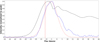Fig. 16.

HI (black) and ¹²CO (blue) profiles extracted from the area 281° < l < 285.5° and −2° < b < 1°. The tangent velocity (−11.35 km s⁻¹) is marked by the vertical red line. The red curve is a fitted Gaussian used to evaluate the velocity of the CO peak (−5.8 km s⁻¹).

The study of the tangent direction to the Carina arm gives us the opportunity to study a part of our Galaxy that is relatively free from foreground and background confusion, enabling us to estimate the star formation activity of this zone.

We evaluate the H₂ mass of the tangent arm section from the ¹²CO(1-0) NANTEN datacube. We extract (281° < l < 285.5°and −2° < b < 1°), integrate the data in the velocity range −20 to +20 km s⁻¹, and evaluate the mass following Heiderman & Evans (2010). For the same area, we evaluate the H₂ mass from the Hi-GAL column density map, keeping only pixels with A_V > 8 mag and the H I mass from the HI4PI column-density maps (established for the same velocity range). The masses are evaluated for a mean distance of 4 kpc and we obtain: M_HI = 3.7 × 10⁶ M_⊙ (Σ_HI = 2.9 M_⊙ pc⁻²), $M_{H_{2}}^{CO} = 7.9$ $M_\mathrm{H_{2}}^{\mathrm{CO}} = 7.9$ × 10⁶ M_⊙ ( $Σ_{H_{2}}^{CO} = 6.3 M_{⊙}$ $\Sigma_\mathrm{H_{2}}^{\mathrm{CO}} = 6.3\,M_\odot$ pc⁻²), and $M_{H_{2}}^{coldens} = 3.9$ $M_\mathrm{H_{2}}^{\mathrm{coldens}} = 3.9$ × 10⁶ M_⊙ ( $Σ_{H_{2}}^{coldens} = 3.1 M_{⊙}$ $\Sigma_\mathrm{H_{2}}^{\mathrm{coldens}}= 3.1\,M_\odot$ pc⁻²) from the CO datacube and the Hi-GAL column density map, respectively. We can see that the M_H₂ calculated from the column density map is in agreement with the total molecular cloud mass calculated from the Miville-Deschênes et al. (2017) catalog ( $M_{H_{2}}^{cat} = 4.4$ $M_\mathrm{H_{2}}^{\mathrm{cat}} = 4.4$ × 10⁶ M_⊙). The difference between $M_{H_{2}}^{CO}$ $M_\mathrm{H_{2}}^{\mathrm{CO}}$ and $M_{H_{2}}^{coldens}$ $M_\mathrm{H_{2}}^{\mathrm{coldens}}$ is expected, as the former includes the more diffuse contribution while the latter represents mostly the densest and structured molecular gas. This allows us to estimate that about 38% of the H₂ mass is structured and that only ∼6.5% is in the form of clumps (the total mass of the clumps being M_clumps = 2.73 × 10⁵ M_⊙). We also estimate the fraction of molecular gas (defined as fmol = Σ_H₂/(Σ_HI + Σ_H₂)) between 0.52 and 0.68.

The Σ_HI, Σ_H₂, and fmol disagree with the expected values (Σ_HI ∼ 6 M_⊙ pc⁻², Σ_H₂ ∼ 2 M_⊙ pc⁻² and fmol ∼ 0.1–0.2) at the galactocentric distance of the region (R ∼ 8.5 kpc) from azimuthally averaged plots in Nakanishi & Sofue (2016), Koda et al. (2016), and Miville-Deschênes et al. (2017). The region seems to be dominated by molecular gas, while the opposite is expected given its Galactic radius. As the variations of fmol can reach 40%–50% for R > 6 kpc (Koda et al. 2016) and if the azimuthally averaged plots represent mainly inter-arm medium, one can interpret the observed values as being due to H I–H₂ conversion in the spiral arm as suggested by Koda et al. (2016). In parallel, Lépine et al. (2011) show that the Carina arm is well traced from CS sources and suggest that it coincides with the corotation radius. Combined with the fact that the corotation radius corresponds to a ring-shaped gap in the radial HI density distribution (Amôres et al. 2009), one could expect that, locally, the H I gas is lower than the general trend.

From the gas masses, using Eq. (3) in Heiderman & Evans (2010) and Bigiel et al. (2008), we estimate a $Σ_{SFR}^{gas}$ $\Sigma_{\mathrm{SFR}}^{\mathrm{gas}}$ of between 0.0025 $_{- 0.0013}^{+ 0.0024}$ $^{+0.0024}_{-0.0013}$ and 0.005 $_{- 0.0021}^{+ 0.0037}$ $^{+0.0037}_{-0.0021}$ M_⊙ yr⁻¹ kpc⁻² from $M_{H_{2}}^{coldens}$ $M_\mathrm{H_{2}}^{\mathrm{coldens}}$ and $M_{H_{2}}^{CO}$ $M_\mathrm{H_{2}}^{\mathrm{CO}}$ , respectively, which can be compared to more direct SFR evaluations. We first compare to the recent SFR as traced by YSOs. To this end, we first evaluated the stellar mass using the candidate YSOs from Kuhn et al. (2021; SPICY catalog) and Marton et al. (2019) within the same spatial area. For the Marton et al. (2019) catalog, we selected here the stars with a probability of higher than 95% of being a YSO, leading to a sample of 3710 objects. In addition, from the SPICY catalog we selected only class I, class II, and flat-spectrum stars with 3.6 μm magnitude brighter than 13.5 (the estimated completeness limit), leading to a sample of 1363 objects. We then cross-matched (1″ cone search) these YSO samples with the Gaia-DR3 distance catalog (Bailer-Jones et al. 2021) and complemented the photometric information (from WISE, 2MASS, and Spitzer catalogs cross-matches). For every star with a distance of between 1.8 and 6.5 kpc, we ran the SED-fitting tool from Robitaille (2017). Following Sewiło et al. (2019), after fitting the models, we counted the number of good fits provided by each model set and the one with the largest number of good fits was selected as the best model set from which the selected best model is the one with the smallest χ². The selected model gave the modeled radius and temperature of the source, from which we evaluated the mass using the zero-age main sequence luminosity–mass relation as recalled by Immer et al. (2012). After concatenating the two samples (taking into account the 135 objects in common), we have a final sample of 3884 YSOs with a distance and therefore a mass estimate. We then followed the method described in Immer et al. (2012), fitting our mass distribution histogram (see Fig. 17) with a curve (ξ = A M^−2.3, where A is the normalisation factor), which follows the form of the Kroupa (2001) IMF for M ≥ 0.5 M_⊙. The fit solves the value of the normalisation factor (A = 4500 ± 665) which, assuming continuous IMF, was used to extrapolate the IMF to the lower masses following the Kroupa (2001) relations for M ≤ 0.5 M_⊙ (see Immer et al. 2012). We then estimated that the total mass of the YSOs within the mass range of 0.01–120 M_⊙ is 21 368 ± 3157 M_⊙. From the histogram, one can note that the lowest-mass and highest-mass objects are missing due to the completeness limit magnitude and saturation effects, while between 2 and 5 M_⊙ the number of sources is overestimated with respect to the curve, which is certainly due to contamination by evolved objects misclassified as YSOs. From these deviations, we can estimate an uncertainty of 10% on the total mass. Assuming that all YSOs that constitute our sample have an average age of 2 ± 1 Myr (Evans 2009), the estimated average recent star formation rate SFR^recent = 0.010 ± 0.007 M_⊙ yr⁻¹, leading to $Σ_{SFR}^{recent}$ $\Sigma_{\mathrm{SFR}}^{\mathrm{recent}}$ = 0.008 ± 0.005 M_⊙ yr⁻¹ kpc⁻².

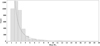Fig. 17.

Distribution of the YSO masses (3884 YSOs). The line represents the Kroupa (2001) IMF that best fits the data.

We can iterate the SFR evaluation from the ionization rate, which gives us the “immediate past” SFR. To this end, for every H II region, we retrieved the radio continuum flux density from the literature and calculated the ionization rate N_Lyc (Eq. (1) from Figueira et al. 2019), adopting the temperature from Caswell & Haynes (1987) when available (else 8000 K is adopted). This led to SFR^imm.past = 0.0053 M_⊙ yr⁻¹ (following the Calzetti 2013 relation between the SFR and N_Lyc) and therefore $Σ_{SFR}^{imm . past}$ $\Sigma_{\mathrm{SFR}}^{\mathrm{imm.past}}$ = 0.0042 M_⊙ yr⁻¹ kpc⁻².

Finally, the SFR was calculated from protostellar clumps following the SFR–clump mass relation given by Elia et al. (2022). This gives us the present SFR: SFR^present = 0.017± 0.0006 M_⊙ yr⁻¹ and $Σ_{SFR}^{present}$ $\Sigma_{\mathrm{SFR}}^{\mathrm{present}}$ = 0.013 ± 0.0005 M_⊙ yr⁻¹ kpc⁻², respectively.

The $Σ_{SFR}^{imm . past}$ $\Sigma_{\mathrm{SFR}}^{\mathrm{imm. past}}$ is in agreement with the $Σ_{SFR}^{gas}$ $\Sigma_{\mathrm{SFR}}^{\mathrm{gas}}$ , suggesting a constant gas inflow in the arm over the typical timescale of T_{(co − Hα)} ∼ 4.3 Myr. The $Σ_{SFR}^{present}$ $\Sigma_{\mathrm{SFR}}^{\mathrm{present}}$ is slightly larger than $Σ_{SFR}^{recent}$ $\Sigma_{\mathrm{SFR}}^{\mathrm{recent}}$ –albeit at the upper bound of the error bar– suggesting a constant SFR over a 2 Myr timescale. The $Σ_{SFR}^{imm . past}$ $\Sigma_{\mathrm{SFR}}^{\mathrm{imm. past}}$ is smaller than $Σ_{SFR}^{recent}$ $\Sigma_{\mathrm{SFR}}^{\mathrm{recent}}$ and $Σ_{SFR}^{present}$ $\Sigma_{\mathrm{SFR}}^{\mathrm{present}}$ suggesting a possible recent burst of star formation.

The SFR values we obtain are between those of the solar neighborhood (Σ_SFR = 0.0024 M_⊙ yr⁻¹ kpc⁻²; Fuchs et al. 2009), which can be considered a quiescent zone, and the most active galactic central molecular zone (with Σ_SFR between 0.046 and 0.14 M_⊙ yr⁻¹ kpc⁻²; Nandakumar et al. 2018; Nguyen et al. 2021; Yusef-Zadeh et al. 2009), and fall inside the normal star-formation quadrant of the Schmidt-Kennicutt relation as defined by Nguyen-Luong et al. (2016), suggesting that the Carina arm tangency has an intermediate or “normal” star-formation activity.

8. Summary and conclusions

We led a study of the Carina arm tangency, performing an analysis of the ionized (Hα) gas kinematics and the star formation in the Galactic plane area with longitudes from 281° to 285.5° and latitudes of between ∼−2.5° and ∼+1°. We first led a detailed analysis of the kinematics and distance of the optical H II regions, combining our Hα data with multiwavelength data from the literature. In particular, we analyzed the Hα velocity field of the two well-known regions RCW 49 and RCW 48, confirming the expansion velocity of ∼20 km s⁻¹ for RCW 49 and a double shell structure for RCW 48, which provides support to the probable wind interaction with a previous mass-loss episode. We show that the Carina arm tangency spread from 2 to 6 kpc in heliocentric distance and from −20 to +20 km s⁻¹ in V_LSR. Our study of the Carina arm tangency allowed us to probe the star formation at ∼1 kpc⁻² scale; we show that the star-formation activity is intermediate in comparison with the quiescient solar neighborhood and the most active central molecular zone.

¹

Retrieved from http://darkclouds.u-gakugei.ac.jp/index.html

²

The Renormalized Unit Weight Error (RUWE) is expected to be around 1.0 for sources where the single-star model provides a good fit to the astrometric observations. A value significantly greater than 1.4 could indicate that the source is non-single or otherwise problematic for the astrometric solution. See the link https://gea.esac.esa.int/archive/documentation/GDR2/

³

http://simbad.u-strasbg.fr/simbad/

⁴

See http://www-wfau.roe.ac.uk/sss/halpha/

Acknowledgments

This work presents results from the European Space Agency (ESA) space mission Gaia. Gaia data are being processed by the Gaia Data Processing and Analysis Consortium (DPAC). Funding for the DPAC is provided by national institutions, in particular the institutions participating in the Gaia MultiLateral Agreement (MLA). The Gaia mission website is https://www.cosmos.esa.int/gaia. The Gaia archive website is https://archives.esac.esa.int/gaia.

References

Amôres, E. B., Lépine, J. R. D., & Mishurov, Y. N. 2009, MNRAS, 400, 1768 [CrossRef] [Google Scholar]
Amram, P., Boulesteix, J., Georgelin, Y. M., et al. 1991, The Messenger, 64, 44 [NASA ADS] [Google Scholar]
Arthur, S. J. 2007, Astrophys. Space Sci. Proc., 1, 183 [NASA ADS] [CrossRef] [Google Scholar]
Arthur, S. J., & Hoare, M. G. 2006, ApJS, 165, 283 [NASA ADS] [CrossRef] [Google Scholar]
Ascenso, J., Alves, J., Beletsky, Y., & Lago, M. T. V. T. 2007, A&A, 466, 137 [NASA ADS] [CrossRef] [EDP Sciences] [Google Scholar]
Bailer-Jones, C. A. L., Rybizki, J., Fouesneau, M., Demleitner, M., & Andrae, R. 2021, AJ, 161, 147 [Google Scholar]
Barnes, P. J., Yonekura, Y., Fukui, Y., et al. 2011, ApJS, 196, 12 [NASA ADS] [CrossRef] [Google Scholar]
Belloni, T., & Mereghetti, S. 1994, A&A, 286, 935 [NASA ADS] [Google Scholar]
Benaglia, P., Romero, G. E., Koribalski, B., & Pollock, A. M. T. 2005, A&A, 440, 743 [NASA ADS] [CrossRef] [EDP Sciences] [Google Scholar]
Benaglia, P., Koribalski, B., Peri, C. S., et al. 2013, A&A, 559, A31 [NASA ADS] [CrossRef] [EDP Sciences] [Google Scholar]
Benjamin, R. A., Churchwell, E., Babler, B. L., et al. 2005, ApJ, 630, L149 [NASA ADS] [CrossRef] [Google Scholar]
Bigay, J. H., Garnier, R., Georgelin, Y. P., & Georgelin, Y. M. 1972, A&A, 18, 301 [NASA ADS] [Google Scholar]
Bigiel, F., Leroy, A., Walter, F., et al. 2008, AJ, 136, 2846 [NASA ADS] [CrossRef] [Google Scholar]
Bock, D. C. J., Large, M. I., & Sadler, E. M. 1999, AJ, 117, 1578 [Google Scholar]
Bovy, J., Allende Prieto, C., Beers, T. C., et al. 2012, ApJ, 759, 131 [NASA ADS] [CrossRef] [Google Scholar]
Brand, J., & Blitz, L. 1993, A&A, 275, 67 [NASA ADS] [Google Scholar]
Brand, J., Blitz, L., Wouterloot, J. G. A., & Kerr, F. J. 1987, A&AS, 68, 1 [NASA ADS] [Google Scholar]
Bronfman, L., Nyman, L. A., & May, J. 1996, A&AS, 115, 81 [Google Scholar]
Brown, C., Dickey, J. M., Dawson, J. R., & McClure-Griffiths, N. M. 2014, ApJS, 211, 29 [NASA ADS] [CrossRef] [Google Scholar]
Buckner, A. S. M., & Froebrich, D. 2013, MNRAS, 436, 1465 [NASA ADS] [CrossRef] [Google Scholar]
Buckner, A. S. M., & Froebrich, D. 2014, MNRAS, 444, 290 [Google Scholar]
Calabretta, M. R., Staveley-Smith, L., & Barnes, D. G. 2014, PASA, 31, e007 [Google Scholar]
Calzetti, D. 2013, in Secular Evolution of Galaxies, eds. J. Falcón-Barroso, & J. H. Knapen (Cambridge University Press), 419 [CrossRef] [Google Scholar]
Cantat-Gaudin, T., Jordi, C., Vallenari, A., et al. 2018, A&A, 618, A93 [NASA ADS] [CrossRef] [EDP Sciences] [Google Scholar]
Capriotti, E. R., & Kozminski, J. F. 2001, PASP, 113, 677 [NASA ADS] [CrossRef] [Google Scholar]
Carraro, G., & Munari, U. 2004, MNRAS, 347, 625 [NASA ADS] [CrossRef] [Google Scholar]
Caswell, J. L., & Haynes, R. F. 1987, A&A, 171, 261 [NASA ADS] [Google Scholar]
Cersosimo, J. C., Mader, S., Figueroa, N. S., et al. 2009, ApJ, 699, 469 [NASA ADS] [CrossRef] [Google Scholar]
Chen, B. Q., Huang, Y., Hou, L. G., et al. 2019, MNRAS, 487, 1400 [NASA ADS] [CrossRef] [Google Scholar]
Chu, Y. H. 1982, ApJ, 254, 578 [CrossRef] [Google Scholar]
Chu, Y.-H. 1988, PASP, 100, 986 [NASA ADS] [CrossRef] [Google Scholar]
Chu, Y. H., Treffers, R. R., & Kwitter, K. B. 1983, ApJS, 53, 937 [NASA ADS] [CrossRef] [Google Scholar]
Churchwell, E., Whitney, B. A., Babler, B. L., et al. 2004, ApJS, 154, 322 [NASA ADS] [CrossRef] [Google Scholar]
Clemens, D. P. 1985, ApJ, 295, 422 [NASA ADS] [CrossRef] [Google Scholar]
Cohen, R. S., Grabelsky, D. A., May, J., et al. 1985, ApJ, 290, L15 [CrossRef] [Google Scholar]
Dame, T. M. 2007, ApJ, 665, L163 [NASA ADS] [CrossRef] [Google Scholar]
Dame, T. M., Hartmann, D., & Thaddeus, P. 2001, ApJ, 547, 792 [Google Scholar]
Deharveng, L., & Maucherat, M. 1974, A&A, 34, 465 [NASA ADS] [Google Scholar]
Dias, W. S., Monteiro, H., Moitinho, A., et al. 2021, MNRAS, 504, 356 [NASA ADS] [CrossRef] [Google Scholar]
Dib, S., Schmeja, S., & Parker, R. J. 2018, MNRAS, 473, 849 [Google Scholar]
Dobashi, K. 2011, PASJ, 63, S1 [NASA ADS] [CrossRef] [Google Scholar]
Dobashi, K., Uehara, H., Kandori, R., et al. 2005, PASJ, 57, S1 [Google Scholar]
Dobashi, K., Marshall, D. J., Shimoikura, T., & Bernard, J.-P. 2013, PASJ, 65, 31 [NASA ADS] [Google Scholar]
Dunne, B. C., Chu, Y.-H., Chen, C. H. R., et al. 2003, ApJ, 590, 306 [NASA ADS] [CrossRef] [Google Scholar]
Dutra, C. M., & Bica, E. 2002, A&A, 383, 631 [NASA ADS] [CrossRef] [EDP Sciences] [Google Scholar]
Dutra, C. M., Bica, E., Soares, J., & Barbuy, B. 2003, A&A, 400, 533 [NASA ADS] [CrossRef] [EDP Sciences] [Google Scholar]
Egusa, F., Sofue, Y., & Nakanishi, H. 2004, PASJ, 56, L45 [NASA ADS] [Google Scholar]
Eilers, A.-C., Hogg, D. W., Rix, H.-W., & Ness, M. K. 2019, ApJ, 871, 120 [Google Scholar]
Elia, D., Molinari, S., Fukui, Y., et al. 2013, ApJ, 772, 45 [NASA ADS] [CrossRef] [Google Scholar]
Elia, D., Merello, M., Molinari, S., et al. 2021, MNRAS, 504, 2742 [NASA ADS] [CrossRef] [Google Scholar]
Elia, D., Molinari, S., Schisano, E., et al. 2022, ApJ, 941, 162 [NASA ADS] [CrossRef] [Google Scholar]
Evans, Neal J. I., Dunham, M. M., Jørgensen, J. K., et al. 2009, ApJS, 181, 321 [NASA ADS] [CrossRef] [Google Scholar]
Figueira, M., López-Calderón, C., Bronfman, L., et al. 2019, A&A, 623, A141 [NASA ADS] [CrossRef] [EDP Sciences] [Google Scholar]
Fuchs, B., Jahreiß, H., & Flynn, C. 2009, AJ, 137, 266 [NASA ADS] [CrossRef] [Google Scholar]
Furukawa, N., Dawson, J. R., Ohama, A., et al. 2009, ApJ, 696, L115 [Google Scholar]
Gaia Collaboration 2020, VizieR Online Data Catalog: I/350 [Google Scholar]
Georgelin, Y. M., Amram, P., Georgelin, Y. P., Le Coarer, E., & Marcelin, M. 1994, A&AS, 108, 513 [NASA ADS] [Google Scholar]
Georgelin, Y. M., Russeil, D., Amram, P., et al. 2000, A&A, 357, 308 [NASA ADS] [Google Scholar]
Georgy, C., Walder, R., Folini, D., et al. 2013, A&A, 559, A69 [NASA ADS] [CrossRef] [EDP Sciences] [Google Scholar]
Göppl, C., & Preibisch, T. 2022, A&A, 660, A11 [NASA ADS] [CrossRef] [EDP Sciences] [Google Scholar]
Grabelsky, D. A., Cohen, R. S., Bronfman, L., Thaddeus, P., & May, J. 1987, ApJ, 315, 122 [CrossRef] [Google Scholar]
Grabelsky, D. A., Cohen, R. S., Bronfman, L., & Thaddeus, P. 1988, ApJ, 331, 181 [NASA ADS] [CrossRef] [Google Scholar]
Greene, T. P., Wilking, B. A., Andre, P., Young, E. T., & Lada, C. J. 1994, ApJ, 434, 614 [NASA ADS] [CrossRef] [Google Scholar]
Gregory, P. C., Vavasour, J. D., Scott, W. K., & Condon, J. J. 1994, ApJS, 90, 173 [NASA ADS] [CrossRef] [Google Scholar]
Hamann, W. R., Gräfener, G., Liermann, A., et al. 2019, A&A, 625, A57 [NASA ADS] [CrossRef] [EDP Sciences] [Google Scholar]
Hanaoka, M., Kaneda, H., Suzuki, T., et al. 2019, PASJ, 71, 6 [NASA ADS] [CrossRef] [Google Scholar]
Heiderman, A., Evans, Neal J. I., Allen, L. E., Huard, T., & Heyer, M., 2010, ApJ, 723, 1019 [NASA ADS] [CrossRef] [Google Scholar]
HI4PI Collaboration (Ben Bekhti, N., et al.) 2016, A&A, 594, A116 [NASA ADS] [CrossRef] [EDP Sciences] [Google Scholar]
Hou, L. G., & Han, J. L. 2014, A&A, 569, A125 [NASA ADS] [CrossRef] [EDP Sciences] [Google Scholar]
Hou, L. G., & Han, J. L. 2015, MNRAS, 454, 626 [Google Scholar]
Hur, H., Park, B.-G., Sung, H., et al. 2015, MNRAS, 446, 3797 [CrossRef] [Google Scholar]
Immer, K., Schuller, F., Omont, A., & Menten, K. M. 2012, A&A, 537, A121 [NASA ADS] [CrossRef] [EDP Sciences] [Google Scholar]
Kang, S.-J., Kerton, C. R., Choi, M., & Kang, M. 2017, ApJ, 845, 21 [CrossRef] [Google Scholar]
Kawata, D., Hunt, J. A. S., Grand, R. J. J., Pasetto, S., & Cropper, M. 2014, MNRAS, 443, 2757 [NASA ADS] [CrossRef] [Google Scholar]
Kharchenko, N. V., Piskunov, A. E., Röser, S., Schilbach, E., & Scholz, R. D. 2005, A&A, 438, 1163 [NASA ADS] [CrossRef] [EDP Sciences] [Google Scholar]
Kharchenko, N. V., Piskunov, A. E., Schilbach, E., Röser, S., & Scholz, R. D. 2012, A&A, 543, A156 [NASA ADS] [CrossRef] [EDP Sciences] [Google Scholar]
Kharchenko, N. V., Piskunov, A. E., Schilbach, E., Röser, S., & Scholz, R. D. 2013, A&A, 558, A53 [NASA ADS] [CrossRef] [EDP Sciences] [Google Scholar]
Koda, J., Scoville, N., & Heyer, M. 2016, ApJ, 823, 76 [CrossRef] [Google Scholar]
Kroupa, P. 2001, MNRAS, 322, 231 [NASA ADS] [CrossRef] [Google Scholar]
Kuchar, T. A., & Clark, F. O. 1997, ApJ, 488, 224 [NASA ADS] [CrossRef] [Google Scholar]
Kuhn, M. A., de Souza, R. S., Krone-Martins, A., et al. 2021, ApJS, 254, 33 [NASA ADS] [CrossRef] [Google Scholar]
Le Coarer, E., Amram, P., Boulesteix, J., et al. 1992, A&A, 257, 389 [NASA ADS] [Google Scholar]
Lenz, D. D., & Ayres, T. R. 1992, PASP, 104, 1104 [NASA ADS] [CrossRef] [Google Scholar]
Lépine, J. R. D., Roman-Lopes, A., Abraham, Z., Junqueira, T. C., & Mishurov, Y. N. 2011, MNRAS, 414, 1607 [NASA ADS] [CrossRef] [Google Scholar]
Levine, E. S., Blitz, L., & Heiles, C. 2006, Science, 312, 1773 [NASA ADS] [CrossRef] [Google Scholar]
Liu, L., & Pang, X. 2019, ApJS, 245, 32 [CrossRef] [Google Scholar]
Loden, L. O., Loden, K., Nordstrom, B., & Sundman, A. 1976, A&AS, 23, 283 [NASA ADS] [Google Scholar]
Louie, M., Koda, J., & Egusa, F. 2013, ApJ, 763, 94 [NASA ADS] [CrossRef] [Google Scholar]
Mackey, J., Haworth, T. J., Gvaramadze, V. V., et al. 2016, A&A, 586, A114 [NASA ADS] [CrossRef] [EDP Sciences] [Google Scholar]
Magakian, T. Y. 2003, A&A, 399, 141 [NASA ADS] [CrossRef] [EDP Sciences] [Google Scholar]
Marshall, D. J., Robin, A. C., Reylé, C., Schultheis, M., & Picaud, S. 2006, A&A, 453, 635 [NASA ADS] [CrossRef] [EDP Sciences] [Google Scholar]
Marston, A. P. 1996, AJ, 112, 2828 [NASA ADS] [CrossRef] [Google Scholar]
Marston, A. P. 2001, ApJ, 563, 875 [NASA ADS] [CrossRef] [Google Scholar]
Marton, G., Ábrahám, P., Szegedi-Elek, E., et al. 2019, MNRAS, 487, 2522 [Google Scholar]
Mattila, K., Juvela, M., & Lehtinen, K. 2007, ApJ, 654, L131 [NASA ADS] [CrossRef] [Google Scholar]
McClure-Griffiths, N. M., Dickey, J. M., Gaensler, B. M., et al. 2005, ApJS, 158, 178 [NASA ADS] [CrossRef] [Google Scholar]
Mège, P., Russeil, D., Zavagno, A., et al. 2021, A&A, 646, A74 [NASA ADS] [CrossRef] [EDP Sciences] [Google Scholar]
Miville-Deschênes, M.-A., Murray, N., & Lee, E. J. 2017, ApJ, 834, 57 [Google Scholar]
Mizuno, A., & Fukui, Y. 2004, ASP Conf. Ser., 317, 59 [NASA ADS] [Google Scholar]
Mohr-Smith, M., Drew, J. E., Napiwotzki, R., et al. 2017, MNRAS, 465, 1807 [Google Scholar]
Moisés, A. P., Damineli, A., Figuerêdo, E., et al. 2011, MNRAS, 411, 705 [CrossRef] [Google Scholar]
Molinari, S., Swinyard, B., Bally, J., et al. 2010, A&A, 518, L100 [NASA ADS] [CrossRef] [EDP Sciences] [Google Scholar]
Mróz, P., Udalski, A., Skowron, D. M., et al. 2019, ApJ, 870, L10 [Google Scholar]
Murphy, T., Mauch, T., Green, A., et al. 2007, MNRAS, 382, 382 [Google Scholar]
Nakanishi, H., & Sofue, Y. 2016, PASJ, 68, 5 [NASA ADS] [CrossRef] [Google Scholar]
Nandakumar, G., Schultheis, M., Feldmeier-Krause, A., et al. 2018, A&A, 609, A109 [NASA ADS] [CrossRef] [EDP Sciences] [Google Scholar]
Naoz, S., & Shaviv, N. J. 2007, New Astron., 12, 410 [NASA ADS] [CrossRef] [Google Scholar]
Nazé, Y., Chu, Y.-H., Points, S. D., et al. 2001, AJ, 122, 921 [CrossRef] [Google Scholar]
Nesterov, V. V., Kuzmin, A. V., Ashimbaeva, N. T., et al. 1995, A&AS, 110, 367 [NASA ADS] [Google Scholar]
Nguyen, H., Rugel, M. R., Menten, K. M., et al. 2021, A&A, 651, A88 [NASA ADS] [CrossRef] [EDP Sciences] [Google Scholar]
Nguyen-Luong, Q., Nguyen, H. V. V., Motte, F., et al. 2016, ApJ, 833, 23 [NASA ADS] [CrossRef] [Google Scholar]
Ohama, A., Dawson, J. R., Furukawa, N., et al. 2010, ApJ, 709, 975 [CrossRef] [Google Scholar]
Otrupcek, R. E., Hartley, M., & Wang, J. S. 2000, PASA, 17, 92 [NASA ADS] [CrossRef] [Google Scholar]
Paladini, R., Ingallinera, A., Agliozzo, C., et al. 2015, ApJ, 813, 24 [CrossRef] [Google Scholar]
Pan, H.-A., Schinnerer, E., Hughes, A., et al. 2022, ApJ, 927, 9 [NASA ADS] [CrossRef] [Google Scholar]
Panagia, N. 1973, AJ, 78, 929 [NASA ADS] [CrossRef] [Google Scholar]
Pilbratt, G. L., Riedinger, J. R., Passvogel, T., et al. 2010, A&A, 518, L1 [NASA ADS] [CrossRef] [EDP Sciences] [Google Scholar]
Povich, M. S., Kuhn, M. A., Getman, K. V., et al. 2013, ApJS, 209, 31 [NASA ADS] [CrossRef] [Google Scholar]
Ragan, S. E., Moore, T. J. T., Eden, D. J., et al. 2016, MNRAS, 462, 3123 [NASA ADS] [CrossRef] [Google Scholar]
Ragan, S. E., Moore, T. J. T., Eden, D. J., et al. 2018, MNRAS, 479, 2361 [NASA ADS] [CrossRef] [Google Scholar]
Rauw, G., Manfroid, J., Gosset, E., et al. 2007, A&A, 463, 981 [NASA ADS] [CrossRef] [EDP Sciences] [Google Scholar]
Reed, B. C. 1998, ApJS, 115, 271 [NASA ADS] [CrossRef] [Google Scholar]
Relaño, M., & Beckman, J. E. 2005, A&A, 430, 911 [NASA ADS] [CrossRef] [EDP Sciences] [Google Scholar]
Roberts, W. W. 1969, ApJ, 158, 123 [NASA ADS] [CrossRef] [Google Scholar]
Robitaille, T. P. 2017, A&A, 600, A11 [NASA ADS] [CrossRef] [EDP Sciences] [Google Scholar]
Rosado, M., Sánchez-Cruces, M., Ambrocio-Cruz, P., & Trejo, D. 2021, MNRAS, 506, 4263 [NASA ADS] [CrossRef] [Google Scholar]
Rozas, M., Richer, M. G., López, J. A., Relaño, M., & Beckman, J. E. 2006, A&A, 455, 549 [NASA ADS] [CrossRef] [EDP Sciences] [Google Scholar]
Russeil, D. 2003, A&A, 397, 133 [CrossRef] [EDP Sciences] [Google Scholar]
Russeil, D., & Castets, A. 2004, A&A, 417, 107 [NASA ADS] [CrossRef] [EDP Sciences] [Google Scholar]
Russeil, D., Georgelin, Y. M., Amram, P., et al. 1998, A&AS, 130, 119 [NASA ADS] [CrossRef] [EDP Sciences] [Google Scholar]
Russeil, D., Adami, C., & Georgelin, Y. M. 2007, A&A, 470, 161 [NASA ADS] [CrossRef] [EDP Sciences] [Google Scholar]
Russeil, D., Zavagno, A., Mège, P., et al. 2017, A&A, 601, L5 [NASA ADS] [CrossRef] [EDP Sciences] [Google Scholar]
Russeil, D., Zavagno, A., Nguyen, A., et al. 2020, A&A, 642, A21 [NASA ADS] [CrossRef] [EDP Sciences] [Google Scholar]
Sánchez-Cruces, M., Rosado, M., Fuentes-Carrera, I., & Ambrocio-Cruz, P. 2018, MNRAS, 473, 1705 [CrossRef] [Google Scholar]
Schisano, E., Molinari, S., Elia, D., et al. 2020, MNRAS, 492, 5420 [Google Scholar]
Sewiło, M., Whitney, B. A., Yung, B. H. K., et al. 2019, ApJS, 240, 26 [CrossRef] [Google Scholar]
Shull, J. M., Darling, J., & Danforth, C. W. 2021, ApJ, 914, 18 [NASA ADS] [CrossRef] [Google Scholar]
Skiff, B. A. 2014, VizieR Online Data Catalog: B/mk [Google Scholar]
Soares, J. B., Bica, E., Ahumada, A. V., & Clariá, J. J. 2008, A&A, 478, 419 [NASA ADS] [CrossRef] [EDP Sciences] [Google Scholar]
Stark, A. A., & Brand, J. 1989, ApJ, 339, 763 [CrossRef] [Google Scholar]
Stark, A. A., & Lee, Y. 2006, ApJ, 641, L113 [NASA ADS] [CrossRef] [Google Scholar]
Tiwari, M., Karim, R., Pound, M. W., et al. 2021, ApJ, 914, 117 [NASA ADS] [CrossRef] [Google Scholar]
Toalá, J. A., Marston, A. P., Guerrero, M. A., Chu, Y. H., & Gruendl, R. A. 2017, ApJ, 846, 76 [CrossRef] [Google Scholar]
Townsley, L. K., Feigelson, E. D., Montmerle, T., et al. 2003, ApJ, 593, 874 [NASA ADS] [CrossRef] [Google Scholar]
Tremblin, P., Anderson, L. D., Didelon, P., et al. 2014, A&A, 568, A4 [NASA ADS] [CrossRef] [EDP Sciences] [Google Scholar]
Urquhart, J. S., Moore, T. J. T., Csengeri, T., et al. 2014, MNRAS, 443, 1555 [Google Scholar]
Vallée, J. P. 2008, AJ, 135, 1301 [CrossRef] [Google Scholar]
Vallée, J. P. 2018, ApJ, 863, 52 [CrossRef] [Google Scholar]
Vallée, J. P. 2020, New Astron., 76 [Google Scholar]
Vallée, J. P. 2021, MNRAS, 506, 523 [CrossRef] [Google Scholar]
Vallée, J. P. 2022, Ap&SS, 367, 26 [CrossRef] [Google Scholar]
van Marle, A. J., Meliani, Z., & Marcowith, A. 2015, A&A, 584, A49 [CrossRef] [EDP Sciences] [Google Scholar]
Velusamy, T., Langer, W. D., Goldsmith, P. F., & Pineda, J. L. 2015, A&A, 578, A135 [NASA ADS] [CrossRef] [EDP Sciences] [Google Scholar]
Wang, H.-F., Chrobáková, Ž., López-Corredoira, M., & Sylos Labini, F. 2023, ApJ, 942, 12 [NASA ADS] [CrossRef] [Google Scholar]
Wenger, T. V., Dawson, J. R., Dickey, J. M., et al. 2021, ApJS, 254, 36 [NASA ADS] [CrossRef] [Google Scholar]
Whiteoak, J. B. Z., & Uchida, K. I. 1997, A&A, 317, 563 [NASA ADS] [Google Scholar]
Williams, R. J. R. 1999, MNRAS, 310, 789 [NASA ADS] [CrossRef] [Google Scholar]
Wilson, T. L., Mezger, P. G., Gardner, F. F., & Milne, D. K. 1970, A&A, 6, 364 [NASA ADS] [Google Scholar]
Xu, Y., Hou, L. G., Bian, S. B., et al. 2021, A&A, 645, L8 [EDP Sciences] [Google Scholar]
Yusef-Zadeh, F., Hewitt, J. W., Arendt, R. G., et al. 2009, ApJ, 702, 178 [Google Scholar]
Zari, E., Rix, H. W., Frankel, N., et al. 2021, A&A, 650, A112 [NASA ADS] [CrossRef] [EDP Sciences] [Google Scholar]
Zeidler, P., Sabbi, E., Nota, A., et al. 2015, AJ, 150, 78 [NASA ADS] [CrossRef] [Google Scholar]
Zeidler, P., Sabbi, E., Nota, A., & McLeod, A. F. 2021, AJ, 161, 140 [NASA ADS] [CrossRef] [Google Scholar]
Zhu, Q., Davies, B., Figer, D. F., & Trombley, C. 2009, ApJ, 702, 929 [NASA ADS] [CrossRef] [Google Scholar]

Appendix A: Additional table

Table A.1.

Clusters and groups

Appendix B: Additional figures

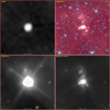Fig. B.1.

Multiview of G281.595-0.969 (FOV: 11.55′ ×11.55′, Galactic coordinates orientation): SUMSS (upper left), Glimpse360 (upper right) with the Spitzer 3.6 μm, Spitzer 4.5 μm, and WISE 12 μm coded in blue, green, and red, respectively, WISE 22 μm (lower left), and Herschel 70 μm (lower right).

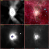Fig. B.2.

Multiview of G281.026-1.180 (FOV: 16.63′ ×16.63′, Galactic coordinates orientation): SUMSS (upper left), Glimpse360 (upper right) with the Spitzer 3.6 μm, Spitzer 4.5 μm, and WISE 12 μm coded in blue, green, and red respectively, WISE 22 μm (lower left), and Herschel 70 μm (lower right).

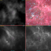Fig. B.3.

Multiview of G282.240-1.099 (FOV: 16.63′ ×16.63′, Galactic coordinates orientation): SUMSS (upper left), Glimpse360 (upper right) with the Spitzer 3.6 μm, Spitzer 4.5 μm, and WISE 12 μm coded in blue, green, and red respectively, WISE 22 μm (lower left), and Herschel 70 μm (lower right).

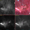Fig. B.4.

Multiview of G282.260-1.810 (FOV: 16.63′ ×16.63′, Galactic coordinates orientation): SUMSS (upper left), Glimpse360 (upper right) with the Spitzer 3.6 μm, Spitzer 4.5 μm, and WISE 12 μm coded in blue, green, and red, respectively, WISE 22 μm (lower left), and Herschel 70 μm (lower right).

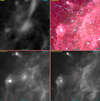Fig. B.5.

Multiview of G282.632-0.853 (FOV: 16.63′ ×16.63′, Galactic coordinates orientation): SUMSS (upper left), Glimpse360 (upper right) with the Spitzer 3.6 μm, Spitzer 4.5 μm, and WISE 12 μm coded in blue, green, and red, respectively, WISE 22 μm (lower left), and Herschel 70 μm (lower right).

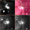Fig. B.6.

Multiview of G283.131-0.984 (FOV: 16.63′ ×16.63′, Galactic coordinates orientation): SUMSS (upper left), Glimpse360 (upper right) with the Spitzer 3.6 μm, Spitzer 4.5 μm, and WISE 12 μm coded in blue, green, and red, respectively, WISE 22 μm (lower left), and Herschel 70 μm (lower right).

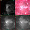Fig. B.7.

Multiview of G283.312-0.566 (FOV: 16.63′ ×16.63′, Galactic coordinates orientation): SUMSS (upper left), Glimpse360 (upper right) with the Spitzer 3.6 μm, Spitzer 4.5 μm, and WISE 12 μm coded in blue, green, and red respectively, WISE 22 μm (lower left), and Herschel 70 μm (lower right).

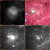Fig. B.8.

Multiview of G283.329-1.050 (FOV: 13.86′ ×13.86′, Galactic coordinates orientation): SUMSS (upper left), Glimpse360 (upper right) with the Spitzer 3.6 μm, Spitzer 4.5 μm, and WISE 12 μm coded in blue, green, and red, respectively, WISE 22 μm (lower left), and Herschel 70 μm (lower right).

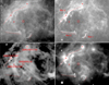Fig. B.9.

Multiview of G283.978-0.92 (Galactic coordinates orientation): Herschel 70 μm (upper left), Spitzer 8μm (upper right), SUMSS (lower left), and WISE 22 μm (lower left). The positions of the radio sources (red crosses), the cluster (red circle) and the rims (underlined by red lines) are overplotted.

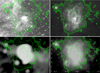Fig. B.10.

Multiview of G285.253-0.053: SHS Hα (upper left), Spitzer 8 μm (upper right), SUMSS (lower left) and Herschel 70 μm (lower right) overplotted with Spitzer 8 μm isocontours. Galactic coordinates are indicated in the lower right image.

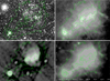Fig. B.11.

Multiview of G281.013-1.528 and G281.162-1.640: SHS Hα (upper left), Herschel 70 μm (upper right), SUMSS (lower left), and WISE 22 μm (lower right) overplotted with Herschel 70 μm isocontours. Galactic coordinates are indicated in the lower right image.

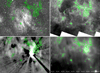Fig. B.12.

Multiview of RCW 46: SHS Hα (upper left), Spitzer 8 μm (upper right), SUMSS (lower left), and AKARI 60 μm (lower right) overplotted with Spitzer 8 μm isocontours. Galactic coordinates are indicated in the lower right image.

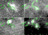Fig. B.13.

Multiview of BRAN 293: SHS Hα (upper left), Spitzer 8μm (upper right), SUMSS (lower left), and WISE 22 μm (lower right) overplotted with Spitzer 8 μm isocontours. Galactic coordinates are indicated in the lower right image.

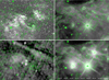Fig. B.14.

Multiview of RCW 47: SHS Hα (upper left), WISE 12 μm (upper right), SUMSS (lower left), and WISE 22 μm (lower right) overplotted with WISE 12 μm isocontours. Galactic coordinates are indicated in the lower right image.

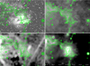Fig. B.15.

Multiview BRAN 299: SHS Hα (upper left), WISE 12 μm (upper right), SUMSS (lower left), and WISE 22 μm (lower right) overplotted with WISE 12 μm isocontours. Galactic coordinates are indicated in the lower right image.

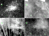Fig. B.16.

Multiview of RCW 50: SHS Hα (upper left), Spitzer 8μm (upper right), SUMSS (lower left)i and AKARI 60μm (lower right) overplotted with Spitzer 8μm isocontours. Galactic coordinates are indicated in the lower right image.

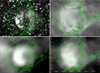Fig. B.17.

Multiview of G284.650-0.484: SHS Hα (upper left), Spitzer 8μm (upper right), SUMSS (lower left), and WISE 22 μm (lower right) overplotted with Spitzer 8 μm isocontours. Galactic coordinates are indicated in the lower right image.

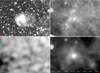Fig. B.18.

Multiview of BRAN 302: SHS Hα (upper left), Spitzer 8 μm (upper right), SUMSS (lower left), and WISE 22 μm (lower right) overplotted with Spitzer 8 μm isocontours. Galactic coordinates are indicated in the lower right image.

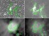Fig. B.19.

Multiview of G284.723+0.313: SHS Hα (upper left), Spitzer 8 μm (upper right), SUMSS (lower left), and WISE 22 μm (lower right) overplotted with Spitzer 8 μm isocontours.

All Tables

Table 1.

Radio sources and H II region information.

In the text

Table A.1.

Clusters and groups

In the text

All Figures

	Fig. 1. General view of the covered area (the J2000 coordinates are in h:m and °:′ format, respectively). This Hα image is a mosaic of the images obtained by adding all the planes of the observed datacubes. The contrast has been chosen to highlight the diffuse emission structures. The names of the main optical H II regions are given in red.
In the text

Fig. 2.

Velocity components (the Galactic coordinate axes are displayed in the figure). The LSR velocity (in km s⁻¹) of the different components is given in yellow (and sorted by decreasing peak intensity). The typical velocity uncertainty is 2 km s⁻¹. For the brightest parts of the H II regions, only the main and intensity-dominating component is given in red (in blue if this component is very broad with FWHM ≥ 40 km s⁻¹).

In the text

Fig. 3.

Av extinction map (Dobashi et al. 2013). The red isocontours are A_Ks of 0.65, 1.55, 2.44, and 3.34 mag, respectively. The blue, green, and cyan contours underline extinction features at 2, 5, and 9.5 kpc respectively, delineated from Marshall et al. (2006) extinction data cubes. The Hα mosaic contour is drawn in black and the Hα emission of the main H II regions is displayed (from the larger-scale SuperCOSMOS Hα Survey (SHS) image) as yellow isocontours.

In the text

Fig. 4.

Significant structures and velocities of RCW 49. Upper panel: mutliwavelength views of RCW 49. The white arrows point to Hα patches with positive velocity and the green contour delineates the arc-like feature. The white dashed circle underlines the circular radio emission feature. Lower panel: velocity (in km s⁻¹) of the different components (sorted by decreasing peak intensities) of the Hα profiles averaged over the areas shown. Coordinates are Galactic (in degrees). Zones dominated by negative (positive) velocity are shown in yellow (green). Values in red have similar intensities while values in blue indicate profiles fitted with a single component. The symbol “ ” indicates that the component has a FWHM ≥ 35 km s⁻¹. The magenta, black, and red stars indicate the positions of Wd2, WR21a, and Collinder 220, respectively.

In the text

Fig. 5.

Representative Hα profiles from the central part of RCW 49 are shown all around the displayed Hα image. The Hα profiles are extracted from the areas delineated on the image. The axes are the V_LSR in km s⁻¹ (X axis) and intensity in arbitrary units (Y axis). The profiles are decomposed into one to three components (labeled from 0 to 2). The solid and dash dotted lines are the observed and the fitted profiles, respectively. All profiles were observed with the P = 2604 interferometer.

In the text

Fig. 6.

Significant structures and velocities of RCW 48. Upper panels: SHS Hα (A), radio continuum SUMSS (843 MHz) (B), Spitzer 8 μm (C), and WISE 22 μm (D) images of RCW 48. Lower panel: Velocity (in km s⁻¹) of the different components (sorted by decreasing peak intensities) of the Hα profiles averaged over the areas shown in the Hα image. The blue arrow is the tangential velocity vector of the star WR18. The red and blue circles delineate the small and large shells discussed in the text, respectively.

In the text

Fig. 7.

Representative Hα profiles from RCW 48 are shown all around the displayed Hα image. The Hα profiles are extracted from the areas delineated on the image. The axes are the V_LSR in km s⁻¹ (X axis) and intensity in arbitrary units (Y axis). The profiles are decomposed into one to three components (labeled “0” to “2”) and night sky lines (labeled “N”), when necessary. The solid and dash dotted lines are the observed and the fitted profiles, respectively. All profiles, except (7) and (8), were observed with the P = 796 interferometer.

In the text

Fig. 8.

Hα profile from RCW50. The profile can be decomposed in three ways (panels 1–3). The axes are the V_LSR in km s⁻¹ (X axis) and intensity in arbitrary units (Y axis). The profile, in addition to the night sky lines (labeled “N”), can be decomposed into either one component (panel 1) or two components (panels 2 and 3), labeled “0” and “1”. The solid and dash dotted lines are the observed and the fitted profiles, respectively.

In the text

Fig. 9.

Longitude–velocity plot of the CO emission from Dame et al. (2001; integrated over latitudes of between 0 and −1.2°) overplotted with HI emission from the HI4PI project (HI4PI Collaboration 2016). In blue, we show the plot of the Carina arm from the Hou & Han (2015) model. The green symbols show the position of the H II regions RCW 46, RCW 48, RCW 49, and G30 (ordered by increasing longitude).

In the text

	Fig. 10. A_G extinction versus distance plot for the six positions along the Galactic plane at l = 280°, 281°, 282°, 283°, 284°, and 285°, respectively.
In the text

Fig. 11.

Histograms of the Gaia distances of different samples. Upper panel: histogram of the Gaia distance of OB star candidates (between 282° and 285.5°) from Mohr-Smith et al. (2017; grey) overplotted with the Xu et al. (2021; blue) and Chen et al. (2019) OB stars samples (red). Lower panel: histogram of the Gaia distances of the OBA star sample from Zari et al. (2021). All stars follow RUWE ≤ 1.4 and π/σ_π > 5).

In the text

	Fig. 12. Pole-on view of the distributions of H II regions and clusters. The full circles are the H II regions (color proportional to log(N_Lyc)), while the cyan and magenta squares are the young (log(age (Myr)) < 8) and old (log(age (Myr)) ≥ 8) clusters, respectively. The position of the Sun is x = 0 and y = 0.
In the text

	Fig. 13. Stellar proper motion for the following samples: Mohr-Smith et al. (2017; black), Xu et al. (2021; blue), Chen et al. (2019; red), and Zari et al. (2021; cyan), respectively.
In the text

	Fig. 14. Distribution of the stellar longitude velocity component (Vlong) of the Mohr-Smith et al. (2017; black) and Zari et al. (2021; red) stellar samples, respectively. The upper and lower panels show the distribution for stars with distances of between 2.2 and 2.7 kpc and farther than 2.8 kpc, respectively.
In the text

Fig. 15.

Distribution of different star formation tracers. Distribution in longitude of: (A) the mean (black line) and the total mass (dashed line) per bin of the molecular clouds catalogued by Miville-Deschênes et al. (2017), (B) the SFF (dashed line) and the SFR (black line) calculated from the Hi-GAL catalog (Elia et al. 2021), and (C) the class I and II YSO counts extracted from the Marton et al. (2019; black line) and Kuhn et al. (2021; dashed line) catalogs, respectively.

In the text

	Fig. 16. HI (black) and ¹²CO (blue) profiles extracted from the area 281° < l < 285.5° and −2° < b < 1°. The tangent velocity (−11.35 km s⁻¹) is marked by the vertical red line. The red curve is a fitted Gaussian used to evaluate the velocity of the CO peak (−5.8 km s⁻¹).
In the text

	Fig. 17. Distribution of the YSO masses (3884 YSOs). The line represents the Kroupa (2001) IMF that best fits the data.
In the text

	Fig. B.1. Multiview of G281.595-0.969 (FOV: 11.55′ ×11.55′, Galactic coordinates orientation): SUMSS (upper left), Glimpse360 (upper right) with the Spitzer 3.6 μm, Spitzer 4.5 μm, and WISE 12 μm coded in blue, green, and red, respectively, WISE 22 μm (lower left), and Herschel 70 μm (lower right).
In the text

	Fig. B.2. Multiview of G281.026-1.180 (FOV: 16.63′ ×16.63′, Galactic coordinates orientation): SUMSS (upper left), Glimpse360 (upper right) with the Spitzer 3.6 μm, Spitzer 4.5 μm, and WISE 12 μm coded in blue, green, and red respectively, WISE 22 μm (lower left), and Herschel 70 μm (lower right).
In the text

	Fig. B.3. Multiview of G282.240-1.099 (FOV: 16.63′ ×16.63′, Galactic coordinates orientation): SUMSS (upper left), Glimpse360 (upper right) with the Spitzer 3.6 μm, Spitzer 4.5 μm, and WISE 12 μm coded in blue, green, and red respectively, WISE 22 μm (lower left), and Herschel 70 μm (lower right).
In the text

	Fig. B.4. Multiview of G282.260-1.810 (FOV: 16.63′ ×16.63′, Galactic coordinates orientation): SUMSS (upper left), Glimpse360 (upper right) with the Spitzer 3.6 μm, Spitzer 4.5 μm, and WISE 12 μm coded in blue, green, and red, respectively, WISE 22 μm (lower left), and Herschel 70 μm (lower right).
In the text

	Fig. B.5. Multiview of G282.632-0.853 (FOV: 16.63′ ×16.63′, Galactic coordinates orientation): SUMSS (upper left), Glimpse360 (upper right) with the Spitzer 3.6 μm, Spitzer 4.5 μm, and WISE 12 μm coded in blue, green, and red, respectively, WISE 22 μm (lower left), and Herschel 70 μm (lower right).
In the text

	Fig. B.6. Multiview of G283.131-0.984 (FOV: 16.63′ ×16.63′, Galactic coordinates orientation): SUMSS (upper left), Glimpse360 (upper right) with the Spitzer 3.6 μm, Spitzer 4.5 μm, and WISE 12 μm coded in blue, green, and red, respectively, WISE 22 μm (lower left), and Herschel 70 μm (lower right).
In the text

	Fig. B.7. Multiview of G283.312-0.566 (FOV: 16.63′ ×16.63′, Galactic coordinates orientation): SUMSS (upper left), Glimpse360 (upper right) with the Spitzer 3.6 μm, Spitzer 4.5 μm, and WISE 12 μm coded in blue, green, and red respectively, WISE 22 μm (lower left), and Herschel 70 μm (lower right).
In the text

	Fig. B.8. Multiview of G283.329-1.050 (FOV: 13.86′ ×13.86′, Galactic coordinates orientation): SUMSS (upper left), Glimpse360 (upper right) with the Spitzer 3.6 μm, Spitzer 4.5 μm, and WISE 12 μm coded in blue, green, and red, respectively, WISE 22 μm (lower left), and Herschel 70 μm (lower right).
In the text

	Fig. B.9. Multiview of G283.978-0.92 (Galactic coordinates orientation): Herschel 70 μm (upper left), Spitzer 8μm (upper right), SUMSS (lower left), and WISE 22 μm (lower left). The positions of the radio sources (red crosses), the cluster (red circle) and the rims (underlined by red lines) are overplotted.
In the text

	Fig. B.10. Multiview of G285.253-0.053: SHS Hα (upper left), Spitzer 8 μm (upper right), SUMSS (lower left) and Herschel 70 μm (lower right) overplotted with Spitzer 8 μm isocontours. Galactic coordinates are indicated in the lower right image.
In the text

	Fig. B.11. Multiview of G281.013-1.528 and G281.162-1.640: SHS Hα (upper left), Herschel 70 μm (upper right), SUMSS (lower left), and WISE 22 μm (lower right) overplotted with Herschel 70 μm isocontours. Galactic coordinates are indicated in the lower right image.
In the text

	Fig. B.12. Multiview of RCW 46: SHS Hα (upper left), Spitzer 8 μm (upper right), SUMSS (lower left), and AKARI 60 μm (lower right) overplotted with Spitzer 8 μm isocontours. Galactic coordinates are indicated in the lower right image.
In the text

	Fig. B.13. Multiview of BRAN 293: SHS Hα (upper left), Spitzer 8μm (upper right), SUMSS (lower left), and WISE 22 μm (lower right) overplotted with Spitzer 8 μm isocontours. Galactic coordinates are indicated in the lower right image.
In the text

	Fig. B.14. Multiview of RCW 47: SHS Hα (upper left), WISE 12 μm (upper right), SUMSS (lower left), and WISE 22 μm (lower right) overplotted with WISE 12 μm isocontours. Galactic coordinates are indicated in the lower right image.
In the text

	Fig. B.15. Multiview BRAN 299: SHS Hα (upper left), WISE 12 μm (upper right), SUMSS (lower left), and WISE 22 μm (lower right) overplotted with WISE 12 μm isocontours. Galactic coordinates are indicated in the lower right image.
In the text

	Fig. B.16. Multiview of RCW 50: SHS Hα (upper left), Spitzer 8μm (upper right), SUMSS (lower left)i and AKARI 60μm (lower right) overplotted with Spitzer 8μm isocontours. Galactic coordinates are indicated in the lower right image.
In the text

	Fig. B.17. Multiview of G284.650-0.484: SHS Hα (upper left), Spitzer 8μm (upper right), SUMSS (lower left), and WISE 22 μm (lower right) overplotted with Spitzer 8 μm isocontours. Galactic coordinates are indicated in the lower right image.
In the text

	Fig. B.18. Multiview of BRAN 302: SHS Hα (upper left), Spitzer 8 μm (upper right), SUMSS (lower left), and WISE 22 μm (lower right) overplotted with Spitzer 8 μm isocontours. Galactic coordinates are indicated in the lower right image.
In the text

	Fig. B.19. Multiview of G284.723+0.313: SHS Hα (upper left), Spitzer 8 μm (upper right), SUMSS (lower left), and WISE 22 μm (lower right) overplotted with Spitzer 8 μm isocontours.
In the text

Current usage metrics show cumulative count of Article Views (full-text article views including HTML views, PDF and ePub downloads, according to the available data) and Abstracts Views on Vision4Press platform.

Data correspond to usage on the plateform after 2015. The current usage metrics is available 48-96 hours after online publication and is updated daily on week days.

Initial download of the metrics may take a while.

[1] Amôres, E. B., Lépine, J. R. D., & Mishurov, Y. N. 2009, MNRAS, 400, 1768 [CrossRef] [Google Scholar]

[2] Amram, P., Boulesteix, J., Georgelin, Y. M., et al. 1991, The Messenger, 64, 44 [NASA ADS] [Google Scholar]

[3] Arthur, S. J. 2007, Astrophys. Space Sci. Proc., 1, 183 [NASA ADS] [CrossRef] [Google Scholar]

[4] Arthur, S. J., & Hoare, M. G. 2006, ApJS, 165, 283 [NASA ADS] [CrossRef] [Google Scholar]

[5] Ascenso, J., Alves, J., Beletsky, Y., & Lago, M. T. V. T. 2007, A&A, 466, 137 [NASA ADS] [CrossRef] [EDP Sciences] [Google Scholar]

[6] Bailer-Jones, C. A. L., Rybizki, J., Fouesneau, M., Demleitner, M., & Andrae, R. 2021, AJ, 161, 147 [Google Scholar]

[7] Barnes, P. J., Yonekura, Y., Fukui, Y., et al. 2011, ApJS, 196, 12 [NASA ADS] [CrossRef] [Google Scholar]

[8] Belloni, T., & Mereghetti, S. 1994, A&A, 286, 935 [NASA ADS] [Google Scholar]

[9] Benaglia, P., Romero, G. E., Koribalski, B., & Pollock, A. M. T. 2005, A&A, 440, 743 [NASA ADS] [CrossRef] [EDP Sciences] [Google Scholar]

[10] Benaglia, P., Koribalski, B., Peri, C. S., et al. 2013, A&A, 559, A31 [NASA ADS] [CrossRef] [EDP Sciences] [Google Scholar]

[11] Benjamin, R. A., Churchwell, E., Babler, B. L., et al. 2005, ApJ, 630, L149 [NASA ADS] [CrossRef] [Google Scholar]

[12] Bigay, J. H., Garnier, R., Georgelin, Y. P., & Georgelin, Y. M. 1972, A&A, 18, 301 [NASA ADS] [Google Scholar]

[13] Bigiel, F., Leroy, A., Walter, F., et al. 2008, AJ, 136, 2846 [NASA ADS] [CrossRef] [Google Scholar]

[14] Bock, D. C. J., Large, M. I., & Sadler, E. M. 1999, AJ, 117, 1578 [Google Scholar]

[15] Bovy, J., Allende Prieto, C., Beers, T. C., et al. 2012, ApJ, 759, 131 [NASA ADS] [CrossRef] [Google Scholar]

[16] Brand, J., & Blitz, L. 1993, A&A, 275, 67 [NASA ADS] [Google Scholar]

[17] Brand, J., Blitz, L., Wouterloot, J. G. A., & Kerr, F. J. 1987, A&AS, 68, 1 [NASA ADS] [Google Scholar]

[18] Bronfman, L., Nyman, L. A., & May, J. 1996, A&AS, 115, 81 [Google Scholar]

[19] Brown, C., Dickey, J. M., Dawson, J. R., & McClure-Griffiths, N. M. 2014, ApJS, 211, 29 [NASA ADS] [CrossRef] [Google Scholar]

[20] Buckner, A. S. M., & Froebrich, D. 2013, MNRAS, 436, 1465 [NASA ADS] [CrossRef] [Google Scholar]

[21] Buckner, A. S. M., & Froebrich, D. 2014, MNRAS, 444, 290 [Google Scholar]

[22] Calabretta, M. R., Staveley-Smith, L., & Barnes, D. G. 2014, PASA, 31, e007 [Google Scholar]

[23] Calzetti, D. 2013, in Secular Evolution of Galaxies, eds. J. Falcón-Barroso, & J. H. Knapen (Cambridge University Press), 419 [CrossRef] [Google Scholar]

[24] Cantat-Gaudin, T., Jordi, C., Vallenari, A., et al. 2018, A&A, 618, A93 [NASA ADS] [CrossRef] [EDP Sciences] [Google Scholar]

[25] Capriotti, E. R., & Kozminski, J. F. 2001, PASP, 113, 677 [NASA ADS] [CrossRef] [Google Scholar]

[26] Carraro, G., & Munari, U. 2004, MNRAS, 347, 625 [NASA ADS] [CrossRef] [Google Scholar]

[27] Caswell, J. L., & Haynes, R. F. 1987, A&A, 171, 261 [NASA ADS] [Google Scholar]

[28] Cersosimo, J. C., Mader, S., Figueroa, N. S., et al. 2009, ApJ, 699, 469 [NASA ADS] [CrossRef] [Google Scholar]

[29] Chen, B. Q., Huang, Y., Hou, L. G., et al. 2019, MNRAS, 487, 1400 [NASA ADS] [CrossRef] [Google Scholar]

[30] Chu, Y. H. 1982, ApJ, 254, 578 [CrossRef] [Google Scholar]

[31] Chu, Y.-H. 1988, PASP, 100, 986 [NASA ADS] [CrossRef] [Google Scholar]

[32] Chu, Y. H., Treffers, R. R., & Kwitter, K. B. 1983, ApJS, 53, 937 [NASA ADS] [CrossRef] [Google Scholar]

[33] Churchwell, E., Whitney, B. A., Babler, B. L., et al. 2004, ApJS, 154, 322 [NASA ADS] [CrossRef] [Google Scholar]

[34] Clemens, D. P. 1985, ApJ, 295, 422 [NASA ADS] [CrossRef] [Google Scholar]

[35] Cohen, R. S., Grabelsky, D. A., May, J., et al. 1985, ApJ, 290, L15 [CrossRef] [Google Scholar]

[36] Dame, T. M. 2007, ApJ, 665, L163 [NASA ADS] [CrossRef] [Google Scholar]

[37] Dame, T. M., Hartmann, D., & Thaddeus, P. 2001, ApJ, 547, 792 [Google Scholar]

[38] Deharveng, L., & Maucherat, M. 1974, A&A, 34, 465 [NASA ADS] [Google Scholar]

[39] Dias, W. S., Monteiro, H., Moitinho, A., et al. 2021, MNRAS, 504, 356 [NASA ADS] [CrossRef] [Google Scholar]

[40] Dib, S., Schmeja, S., & Parker, R. J. 2018, MNRAS, 473, 849 [Google Scholar]

[41] Dobashi, K. 2011, PASJ, 63, S1 [NASA ADS] [CrossRef] [Google Scholar]

[42] Dobashi, K., Uehara, H., Kandori, R., et al. 2005, PASJ, 57, S1 [Google Scholar]

[43] Dobashi, K., Marshall, D. J., Shimoikura, T., & Bernard, J.-P. 2013, PASJ, 65, 31 [NASA ADS] [Google Scholar]

[44] Dunne, B. C., Chu, Y.-H., Chen, C. H. R., et al. 2003, ApJ, 590, 306 [NASA ADS] [CrossRef] [Google Scholar]

[45] Dutra, C. M., & Bica, E. 2002, A&A, 383, 631 [NASA ADS] [CrossRef] [EDP Sciences] [Google Scholar]

[46] Dutra, C. M., Bica, E., Soares, J., & Barbuy, B. 2003, A&A, 400, 533 [NASA ADS] [CrossRef] [EDP Sciences] [Google Scholar]

[47] Egusa, F., Sofue, Y., & Nakanishi, H. 2004, PASJ, 56, L45 [NASA ADS] [Google Scholar]

[48] Eilers, A.-C., Hogg, D. W., Rix, H.-W., & Ness, M. K. 2019, ApJ, 871, 120 [Google Scholar]

[49] Elia, D., Molinari, S., Fukui, Y., et al. 2013, ApJ, 772, 45 [NASA ADS] [CrossRef] [Google Scholar]

[50] Elia, D., Merello, M., Molinari, S., et al. 2021, MNRAS, 504, 2742 [NASA ADS] [CrossRef] [Google Scholar]

[51] Elia, D., Molinari, S., Schisano, E., et al. 2022, ApJ, 941, 162 [NASA ADS] [CrossRef] [Google Scholar]

[52] Evans, Neal J. I., Dunham, M. M., Jørgensen, J. K., et al. 2009, ApJS, 181, 321 [NASA ADS] [CrossRef] [Google Scholar]

[53] Figueira, M., López-Calderón, C., Bronfman, L., et al. 2019, A&A, 623, A141 [NASA ADS] [CrossRef] [EDP Sciences] [Google Scholar]

[54] Fuchs, B., Jahreiß, H., & Flynn, C. 2009, AJ, 137, 266 [NASA ADS] [CrossRef] [Google Scholar]

[55] Furukawa, N., Dawson, J. R., Ohama, A., et al. 2009, ApJ, 696, L115 [Google Scholar]

[56] Gaia Collaboration 2020, VizieR Online Data Catalog: I/350 [Google Scholar]

[57] Georgelin, Y. M., Amram, P., Georgelin, Y. P., Le Coarer, E., & Marcelin, M. 1994, A&AS, 108, 513 [NASA ADS] [Google Scholar]

[58] Georgelin, Y. M., Russeil, D., Amram, P., et al. 2000, A&A, 357, 308 [NASA ADS] [Google Scholar]

[59] Georgy, C., Walder, R., Folini, D., et al. 2013, A&A, 559, A69 [NASA ADS] [CrossRef] [EDP Sciences] [Google Scholar]

[60] Göppl, C., & Preibisch, T. 2022, A&A, 660, A11 [NASA ADS] [CrossRef] [EDP Sciences] [Google Scholar]

[61] Grabelsky, D. A., Cohen, R. S., Bronfman, L., Thaddeus, P., & May, J. 1987, ApJ, 315, 122 [CrossRef] [Google Scholar]

[62] Grabelsky, D. A., Cohen, R. S., Bronfman, L., & Thaddeus, P. 1988, ApJ, 331, 181 [NASA ADS] [CrossRef] [Google Scholar]

[63] Greene, T. P., Wilking, B. A., Andre, P., Young, E. T., & Lada, C. J. 1994, ApJ, 434, 614 [NASA ADS] [CrossRef] [Google Scholar]

[64] Gregory, P. C., Vavasour, J. D., Scott, W. K., & Condon, J. J. 1994, ApJS, 90, 173 [NASA ADS] [CrossRef] [Google Scholar]

[65] Hamann, W. R., Gräfener, G., Liermann, A., et al. 2019, A&A, 625, A57 [NASA ADS] [CrossRef] [EDP Sciences] [Google Scholar]

[66] Hanaoka, M., Kaneda, H., Suzuki, T., et al. 2019, PASJ, 71, 6 [NASA ADS] [CrossRef] [Google Scholar]

[67] Heiderman, A., Evans, Neal J. I., Allen, L. E., Huard, T., & Heyer, M., 2010, ApJ, 723, 1019 [NASA ADS] [CrossRef] [Google Scholar]

[68] HI4PI Collaboration (Ben Bekhti, N., et al.) 2016, A&A, 594, A116 [NASA ADS] [CrossRef] [EDP Sciences] [Google Scholar]

[69] Hou, L. G., & Han, J. L. 2014, A&A, 569, A125 [NASA ADS] [CrossRef] [EDP Sciences] [Google Scholar]

[70] Hou, L. G., & Han, J. L. 2015, MNRAS, 454, 626 [Google Scholar]

[71] Hur, H., Park, B.-G., Sung, H., et al. 2015, MNRAS, 446, 3797 [CrossRef] [Google Scholar]

[72] Immer, K., Schuller, F., Omont, A., & Menten, K. M. 2012, A&A, 537, A121 [NASA ADS] [CrossRef] [EDP Sciences] [Google Scholar]

[73] Kang, S.-J., Kerton, C. R., Choi, M., & Kang, M. 2017, ApJ, 845, 21 [CrossRef] [Google Scholar]

[74] Kawata, D., Hunt, J. A. S., Grand, R. J. J., Pasetto, S., & Cropper, M. 2014, MNRAS, 443, 2757 [NASA ADS] [CrossRef] [Google Scholar]

[75] Kharchenko, N. V., Piskunov, A. E., Röser, S., Schilbach, E., & Scholz, R. D. 2005, A&A, 438, 1163 [NASA ADS] [CrossRef] [EDP Sciences] [Google Scholar]

[76] Kharchenko, N. V., Piskunov, A. E., Schilbach, E., Röser, S., & Scholz, R. D. 2012, A&A, 543, A156 [NASA ADS] [CrossRef] [EDP Sciences] [Google Scholar]

[77] Kharchenko, N. V., Piskunov, A. E., Schilbach, E., Röser, S., & Scholz, R. D. 2013, A&A, 558, A53 [NASA ADS] [CrossRef] [EDP Sciences] [Google Scholar]

[78] Koda, J., Scoville, N., & Heyer, M. 2016, ApJ, 823, 76 [CrossRef] [Google Scholar]

[79] Kroupa, P. 2001, MNRAS, 322, 231 [NASA ADS] [CrossRef] [Google Scholar]

[80] Kuchar, T. A., & Clark, F. O. 1997, ApJ, 488, 224 [NASA ADS] [CrossRef] [Google Scholar]

[81] Kuhn, M. A., de Souza, R. S., Krone-Martins, A., et al. 2021, ApJS, 254, 33 [NASA ADS] [CrossRef] [Google Scholar]

[82] Le Coarer, E., Amram, P., Boulesteix, J., et al. 1992, A&A, 257, 389 [NASA ADS] [Google Scholar]

[83] Lenz, D. D., & Ayres, T. R. 1992, PASP, 104, 1104 [NASA ADS] [CrossRef] [Google Scholar]

[84] Lépine, J. R. D., Roman-Lopes, A., Abraham, Z., Junqueira, T. C., & Mishurov, Y. N. 2011, MNRAS, 414, 1607 [NASA ADS] [CrossRef] [Google Scholar]

[85] Levine, E. S., Blitz, L., & Heiles, C. 2006, Science, 312, 1773 [NASA ADS] [CrossRef] [Google Scholar]

[86] Liu, L., & Pang, X. 2019, ApJS, 245, 32 [CrossRef] [Google Scholar]

[87] Loden, L. O., Loden, K., Nordstrom, B., & Sundman, A. 1976, A&AS, 23, 283 [NASA ADS] [Google Scholar]

[88] Louie, M., Koda, J., & Egusa, F. 2013, ApJ, 763, 94 [NASA ADS] [CrossRef] [Google Scholar]

[89] Mackey, J., Haworth, T. J., Gvaramadze, V. V., et al. 2016, A&A, 586, A114 [NASA ADS] [CrossRef] [EDP Sciences] [Google Scholar]

[90] Magakian, T. Y. 2003, A&A, 399, 141 [NASA ADS] [CrossRef] [EDP Sciences] [Google Scholar]

[91] Marshall, D. J., Robin, A. C., Reylé, C., Schultheis, M., & Picaud, S. 2006, A&A, 453, 635 [NASA ADS] [CrossRef] [EDP Sciences] [Google Scholar]

[92] Marston, A. P. 1996, AJ, 112, 2828 [NASA ADS] [CrossRef] [Google Scholar]

[93] Marston, A. P. 2001, ApJ, 563, 875 [NASA ADS] [CrossRef] [Google Scholar]

[94] Marton, G., Ábrahám, P., Szegedi-Elek, E., et al. 2019, MNRAS, 487, 2522 [Google Scholar]

[95] Mattila, K., Juvela, M., & Lehtinen, K. 2007, ApJ, 654, L131 [NASA ADS] [CrossRef] [Google Scholar]

[96] McClure-Griffiths, N. M., Dickey, J. M., Gaensler, B. M., et al. 2005, ApJS, 158, 178 [NASA ADS] [CrossRef] [Google Scholar]

[97] Mège, P., Russeil, D., Zavagno, A., et al. 2021, A&A, 646, A74 [NASA ADS] [CrossRef] [EDP Sciences] [Google Scholar]

[98] Miville-Deschênes, M.-A., Murray, N., & Lee, E. J. 2017, ApJ, 834, 57 [Google Scholar]

[99] Mizuno, A., & Fukui, Y. 2004, ASP Conf. Ser., 317, 59 [NASA ADS] [Google Scholar]

[100] Mohr-Smith, M., Drew, J. E., Napiwotzki, R., et al. 2017, MNRAS, 465, 1807 [Google Scholar]

[101] Moisés, A. P., Damineli, A., Figuerêdo, E., et al. 2011, MNRAS, 411, 705 [CrossRef] [Google Scholar]

[102] Molinari, S., Swinyard, B., Bally, J., et al. 2010, A&A, 518, L100 [NASA ADS] [CrossRef] [EDP Sciences] [Google Scholar]

[103] Mróz, P., Udalski, A., Skowron, D. M., et al. 2019, ApJ, 870, L10 [Google Scholar]

[104] Murphy, T., Mauch, T., Green, A., et al. 2007, MNRAS, 382, 382 [Google Scholar]

[105] Nakanishi, H., & Sofue, Y. 2016, PASJ, 68, 5 [NASA ADS] [CrossRef] [Google Scholar]

[106] Nandakumar, G., Schultheis, M., Feldmeier-Krause, A., et al. 2018, A&A, 609, A109 [NASA ADS] [CrossRef] [EDP Sciences] [Google Scholar]

[107] Naoz, S., & Shaviv, N. J. 2007, New Astron., 12, 410 [NASA ADS] [CrossRef] [Google Scholar]

[108] Nazé, Y., Chu, Y.-H., Points, S. D., et al. 2001, AJ, 122, 921 [CrossRef] [Google Scholar]

[109] Nesterov, V. V., Kuzmin, A. V., Ashimbaeva, N. T., et al. 1995, A&AS, 110, 367 [NASA ADS] [Google Scholar]

[110] Nguyen, H., Rugel, M. R., Menten, K. M., et al. 2021, A&A, 651, A88 [NASA ADS] [CrossRef] [EDP Sciences] [Google Scholar]

[111] Nguyen-Luong, Q., Nguyen, H. V. V., Motte, F., et al. 2016, ApJ, 833, 23 [NASA ADS] [CrossRef] [Google Scholar]

[112] Ohama, A., Dawson, J. R., Furukawa, N., et al. 2010, ApJ, 709, 975 [CrossRef] [Google Scholar]

[113] Otrupcek, R. E., Hartley, M., & Wang, J. S. 2000, PASA, 17, 92 [NASA ADS] [CrossRef] [Google Scholar]

[114] Paladini, R., Ingallinera, A., Agliozzo, C., et al. 2015, ApJ, 813, 24 [CrossRef] [Google Scholar]

[115] Pan, H.-A., Schinnerer, E., Hughes, A., et al. 2022, ApJ, 927, 9 [NASA ADS] [CrossRef] [Google Scholar]

[116] Panagia, N. 1973, AJ, 78, 929 [NASA ADS] [CrossRef] [Google Scholar]

[117] Pilbratt, G. L., Riedinger, J. R., Passvogel, T., et al. 2010, A&A, 518, L1 [NASA ADS] [CrossRef] [EDP Sciences] [Google Scholar]

[118] Povich, M. S., Kuhn, M. A., Getman, K. V., et al. 2013, ApJS, 209, 31 [NASA ADS] [CrossRef] [Google Scholar]

[119] Ragan, S. E., Moore, T. J. T., Eden, D. J., et al. 2016, MNRAS, 462, 3123 [NASA ADS] [CrossRef] [Google Scholar]

[120] Ragan, S. E., Moore, T. J. T., Eden, D. J., et al. 2018, MNRAS, 479, 2361 [NASA ADS] [CrossRef] [Google Scholar]

[121] Rauw, G., Manfroid, J., Gosset, E., et al. 2007, A&A, 463, 981 [NASA ADS] [CrossRef] [EDP Sciences] [Google Scholar]

[122] Reed, B. C. 1998, ApJS, 115, 271 [NASA ADS] [CrossRef] [Google Scholar]

[123] Relaño, M., & Beckman, J. E. 2005, A&A, 430, 911 [NASA ADS] [CrossRef] [EDP Sciences] [Google Scholar]

[124] Roberts, W. W. 1969, ApJ, 158, 123 [NASA ADS] [CrossRef] [Google Scholar]

[125] Robitaille, T. P. 2017, A&A, 600, A11 [NASA ADS] [CrossRef] [EDP Sciences] [Google Scholar]

[126] Rosado, M., Sánchez-Cruces, M., Ambrocio-Cruz, P., & Trejo, D. 2021, MNRAS, 506, 4263 [NASA ADS] [CrossRef] [Google Scholar]

[127] Rozas, M., Richer, M. G., López, J. A., Relaño, M., & Beckman, J. E. 2006, A&A, 455, 549 [NASA ADS] [CrossRef] [EDP Sciences] [Google Scholar]

[128] Russeil, D. 2003, A&A, 397, 133 [CrossRef] [EDP Sciences] [Google Scholar]

[129] Russeil, D., & Castets, A. 2004, A&A, 417, 107 [NASA ADS] [CrossRef] [EDP Sciences] [Google Scholar]

[130] Russeil, D., Georgelin, Y. M., Amram, P., et al. 1998, A&AS, 130, 119 [NASA ADS] [CrossRef] [EDP Sciences] [Google Scholar]

[131] Russeil, D., Adami, C., & Georgelin, Y. M. 2007, A&A, 470, 161 [NASA ADS] [CrossRef] [EDP Sciences] [Google Scholar]

[132] Russeil, D., Zavagno, A., Mège, P., et al. 2017, A&A, 601, L5 [NASA ADS] [CrossRef] [EDP Sciences] [Google Scholar]

[133] Russeil, D., Zavagno, A., Nguyen, A., et al. 2020, A&A, 642, A21 [NASA ADS] [CrossRef] [EDP Sciences] [Google Scholar]

[134] Sánchez-Cruces, M., Rosado, M., Fuentes-Carrera, I., & Ambrocio-Cruz, P. 2018, MNRAS, 473, 1705 [CrossRef] [Google Scholar]

[135] Schisano, E., Molinari, S., Elia, D., et al. 2020, MNRAS, 492, 5420 [Google Scholar]

[136] Sewiło, M., Whitney, B. A., Yung, B. H. K., et al. 2019, ApJS, 240, 26 [CrossRef] [Google Scholar]

[137] Shull, J. M., Darling, J., & Danforth, C. W. 2021, ApJ, 914, 18 [NASA ADS] [CrossRef] [Google Scholar]

[138] Skiff, B. A. 2014, VizieR Online Data Catalog: B/mk [Google Scholar]

[139] Soares, J. B., Bica, E., Ahumada, A. V., & Clariá, J. J. 2008, A&A, 478, 419 [NASA ADS] [CrossRef] [EDP Sciences] [Google Scholar]

[140] Stark, A. A., & Brand, J. 1989, ApJ, 339, 763 [CrossRef] [Google Scholar]

[141] Stark, A. A., & Lee, Y. 2006, ApJ, 641, L113 [NASA ADS] [CrossRef] [Google Scholar]

[142] Tiwari, M., Karim, R., Pound, M. W., et al. 2021, ApJ, 914, 117 [NASA ADS] [CrossRef] [Google Scholar]

[143] Toalá, J. A., Marston, A. P., Guerrero, M. A., Chu, Y. H., & Gruendl, R. A. 2017, ApJ, 846, 76 [CrossRef] [Google Scholar]

[144] Townsley, L. K., Feigelson, E. D., Montmerle, T., et al. 2003, ApJ, 593, 874 [NASA ADS] [CrossRef] [Google Scholar]

[145] Tremblin, P., Anderson, L. D., Didelon, P., et al. 2014, A&A, 568, A4 [NASA ADS] [CrossRef] [EDP Sciences] [Google Scholar]

[146] Urquhart, J. S., Moore, T. J. T., Csengeri, T., et al. 2014, MNRAS, 443, 1555 [Google Scholar]

[147] Vallée, J. P. 2008, AJ, 135, 1301 [CrossRef] [Google Scholar]

[148] Vallée, J. P. 2018, ApJ, 863, 52 [CrossRef] [Google Scholar]

[149] Vallée, J. P. 2020, New Astron., 76 [Google Scholar]

[150] Vallée, J. P. 2021, MNRAS, 506, 523 [CrossRef] [Google Scholar]

[151] Vallée, J. P. 2022, Ap&SS, 367, 26 [CrossRef] [Google Scholar]

[152] van Marle, A. J., Meliani, Z., & Marcowith, A. 2015, A&A, 584, A49 [CrossRef] [EDP Sciences] [Google Scholar]

[153] Velusamy, T., Langer, W. D., Goldsmith, P. F., & Pineda, J. L. 2015, A&A, 578, A135 [NASA ADS] [CrossRef] [EDP Sciences] [Google Scholar]

[154] Wang, H.-F., Chrobáková, Ž., López-Corredoira, M., & Sylos Labini, F. 2023, ApJ, 942, 12 [NASA ADS] [CrossRef] [Google Scholar]

[155] Wenger, T. V., Dawson, J. R., Dickey, J. M., et al. 2021, ApJS, 254, 36 [NASA ADS] [CrossRef] [Google Scholar]

[156] Whiteoak, J. B. Z., & Uchida, K. I. 1997, A&A, 317, 563 [NASA ADS] [Google Scholar]

[157] Williams, R. J. R. 1999, MNRAS, 310, 789 [NASA ADS] [CrossRef] [Google Scholar]

[158] Wilson, T. L., Mezger, P. G., Gardner, F. F., & Milne, D. K. 1970, A&A, 6, 364 [NASA ADS] [Google Scholar]

[159] Xu, Y., Hou, L. G., Bian, S. B., et al. 2021, A&A, 645, L8 [EDP Sciences] [Google Scholar]

[160] Yusef-Zadeh, F., Hewitt, J. W., Arendt, R. G., et al. 2009, ApJ, 702, 178 [Google Scholar]

[161] Zari, E., Rix, H. W., Frankel, N., et al. 2021, A&A, 650, A112 [NASA ADS] [CrossRef] [EDP Sciences] [Google Scholar]

[162] Zeidler, P., Sabbi, E., Nota, A., et al. 2015, AJ, 150, 78 [NASA ADS] [CrossRef] [Google Scholar]

[163] Zeidler, P., Sabbi, E., Nota, A., & McLeod, A. F. 2021, AJ, 161, 140 [NASA ADS] [CrossRef] [Google Scholar]

[164] Zhu, Q., Davies, B., Figer, D. F., & Trombley, C. 2009, ApJ, 702, 929 [NASA ADS] [CrossRef] [Google Scholar]

A deep Hα survey of the Carina tangent arm direction⋆

1. Introduction

2. Data

2.1. Hα observations

2.2. Other data sets

3. Hα data analysis

3.1. Diffuse emission and extinction

3.2. H II regions kinematics and distance

3.2.1. Radio H II regions

3.2.2. Optical (Hα) H II regions

4. Characterization of the Carina arm tangency

5. Stellar kinematics at the Carina arm tangency

6. Star formation across the arm tangency

7. Star-formation activity

8. Summary and conclusions

Acknowledgments

References

Appendix A: Additional table

Appendix B: Additional figures

All Tables

All Figures

A deep Hα survey of the Carina tangent arm direction^⋆