| Issue |
A&A
Volume 680, December 2023
Solar Orbiter First Results (Nominal Mission Phase)
|
|
|---|---|---|
| Article Number | A90 | |
| Number of page(s) | 18 | |
| Section | The Sun and the Heliosphere | |
| DOI | https://doi.org/10.1051/0004-6361/202346881 | |
| Published online | 15 December 2023 | |
Analysis of the first coronagraphic multi-band observations of a sungrazing comet
1
INAF – Turin Astrophysical Observatory, Turin, Italy
e-mail: This email address is being protected from spambots. You need JavaScript enabled to view it.
2
University of Turin – Physics Department, Turin, Italy
3
U.S. Naval Research Laboratory, Washington, D.C., USA
4
Project Pluto, Bowdoinham, ME 04008, USA
5
Physics Department, U.S. Naval Academy, 572C Holloway Rd, Annapolis, MD 21402, USA
6
University of Padova – Physics and Astronomy Department “Galileo Galilei”, Padua, Italy
7
CNR – Istituto di Fotonica e Nanotecnologie, Padua, Italy
8
INAF – Padova Astronomical Observatory, Vicolo dell’Osservatorio 5, 35122 Padova, Italy
9
University of Calabria – Physics Department, Cosenza, Italy
10
Harvard-Smithsonian Center for Astrophysics, Cambridge, MA, USA
11
University of Florence – Physics and Astronomy Department, Florence, Italy
12
INAF – Arcetri Astrophysical Observatory, Largo Enrico Fermi 5, 50125 Florence, Italy
13
Adnet Systems, Inc., NASA Goddard Space Flight Center, Greenbelt, MD, USA
14
INAF – Capodimonte Astronomical Observatory, Salita Moiariello 16, 80131 Naples, Italy
15
INAF – Catania Astrophysical Observatory, Catania, Italy
16
Max-Planck-Institut für Sonnensystemforschung, Göttingen, Germany
17
University of Catania – Physics and Astronomy Department “Ettore Majorana”, Catania, Italy
18
Astronomical Institute of the Czech Academy of Sciences, Ondřejov, Czech Republic
19
INAF – Trieste Astronomical Observatory, Trieste, Italy
20
Southwest Research Institute, 1050 Walnut Street Suite 300, Boulder, CO 80302, USA
21
Italian Space Agency, Rome, Italy
22
INAF – Istituto di Astrofisica Spaziale e Fisica Cosmica, Milan, Italy
Received:
12
May
2023
Accepted:
19
September
2023
Abstract
Context. Between 24 and 25 December 2021 a sungrazing comet (SOHO-4341) approached the Sun, being observed by “classical” visible light (VL) coronagraphs on board the SOHO and STEREO missions, and also by the innovative Metis coronagraph on board the ESA-NASA Solar Orbiter mission in the VL and ultraviolet (UV H I Lyman-α) band.
Aims. We show how VL data acquired by the Metis coronagraph can be combined with those provided by other space-based coronagraphs to reconstruct the comet orbit, but also to provide information on the dust composition from the polarized VL emission. Moreover, we show how the UV emission can be employed to measure local plasma parameters of the ambient solar wind.
Methods. By using the comet positions tracked with VL Metis images (with spatial resolution that is four times better than UV), the UV images (with a time cadence that is five times faster than VL) have been coaligned to maximize the signal-to-noise ratio in the UV band. The local electron density ne was measured from the observed exponential decay of the UV Lyman-α intensity along the tail, while the solar wind speed vwind was measured from the UV Lyman-α tail inclination with respect to the cometary orbital path deprojected in 3D. Moreover, the proton kinetic temperature Tk was also obtained by the aperture angle of the UV Lyman-α tail.
Results. When the comet was at an average heliocentric distance of 14.3 R⊙, the comet had a radial speed of 155 km s−1 and a tangential speed of 59 km s−1. The comet had a UV Lyman-α tail extending in the anti-solar direction over more than 1.5 R⊙. From the analysis of the tail shape in UV we obtained the local solar wind speed (vwind = 190 km s−1), electron density (ne = 1.5 × 104 cm−3), and proton temperature (Tk = 1.2 × 10⁶ K). Moreover, theoretical analysis of the measured UV Lyman-α intensity allowed us to estimate the radius of the cometary nucleus (Rcom = 65 m) and the water outgassing rate (QH2O = 4.8 × 1028 molec s−1).
Conclusions. These results show that sungrazing comets are unique “local probes” for the ambient coronal plasma, providing measurements that are not as affected by the line-of-sight integration effects as those provided by remote sensing instruments, in regions of the Heliosphere that are not explored in situ by the ongoing space missions.
Key words: comets: general / solar wind / Sun: corona / Sun: UV radiation / methods: data analysis
© The Authors 2023
 Open Access article, published by EDP Sciences, under the terms of the Creative Commons Attribution License (https://creativecommons.org/licenses/by/4.0), which permits unrestricted use, distribution, and reproduction in any medium, provided the original work is properly cited.
This article is published in open access under the Subscribe to Open model. This email address is being protected from spambots. You need JavaScript enabled to view it. to support open access publication.
1. Introduction
One of the surprising discoveries of the modern space-based heliophysics era is the existence of a near-continuous stream of small visible comets with perihelion very close to the Sun (e.g., Biesecker et al. 2002; Marsden 2005; Battams & Knight 2017; Jones et al. 2018). More than 4600 such comets have now been discovered1, mostly with the Large Angle Spectrometric Coronagraph (LASCO) coronagraphs on board the Solar and Heliospheric Observatory (SOHO; see Battams & Knight 2017), but also with the COR1 and COR2 coronagraphs on board the SOlar Terrestrial RElations Observatory (STEREO) allowing 3D reconstructions of cometary tails (e.g., Thompson 2009; Sekanina & Chodas 2012). In the vast majority of the cases, these comets are members of the well-known Kreutz group of sungrazing comets, which includes several historically bright naked-eye comets (e.g., Marsden 1989; Sekanina & Chodas 2004). They are thought to have been produced by fragmentation via the tidal forces of a large comet at the previous perihelion passage as they are too small to survive the perihelion passage during which they are observed (Sekanina 2002; Sekanina & Chodas 2004).
Since the vast majority of individual Kreutz comets are not known to exist prior to their appearance in SOHO or STEREO images, and the duration of observability is typically only a few hours and rarely more than a day, only a few dedicated studies of individual objects have been conducted. In about a dozen cases the LASCO team measured comet positions in time and obtained the orbital solutions to predict the positions relative to the Sun; the UVCS team was able to position the spectrograph slit along the predicted comet trajectory to obtain ultraviolet (UV) spectra (see review by Bemporad et al. 2007). The combination of observations in the visible light (VL) and the UV is particularly interesting because it allows the estimate of the comet nucleus size and the study of the evolution of both the dust and ion tails, and hence the chemical composition of these comets, and possible fragmentation events.
For instance, after the first study by Raymond et al. (1998) dealing with the possible bow-shock associated with the sungrazer C/1996 Y1, Uzzo et al. (2001) studied sungrazer comet C/2000 C6 and found evidence of comet fragmentation processes going on as the comet approached the Sun. Bemporad et al. (2005) analyzed observations of the sungrazer C/2001 C2 and also found the evidence of nucleus fragmentation and a possible signature of additional H atoms produced via charge exchange with sublimation products from pyroxene dust grains. Giordano et al. (2015) studied the sungrazing comet C/2002 S2 and found that Lyman-α continued to brighten, even as the optical brightness faded rapidly as the comet approached the Sun. They interpreted this phenomenon as an indication that the outgassing continued to increase, but that the dust grains sublimated very rapidly due to the intense solar radiation. A comparison of UV emission lines with the optical brightness of observations of comet C/2011 W3 (Lovejoy) was used to determine the composition and sublimation rates of the dust (Raymond et al. 2018). Since the fields of view of the optical and UV instruments on SOHO and STEREO do not overlap, previous studies could not make direct simultaneous comparisons between data sets.
We report here on the first ever simultaneous imaging observations of a Kreutz comet at UV and VL wavelengths, made serendipitously by the Metis instrument (Antonucci et al. 2020; Fineschi et al. 2020; Romoli et al. 2021) on board the ESA-NASA Solar Orbiter mission (Müller et al. 2020). The comet, designated SOHO-4341 by the Sungrazer project and not yet given an official IAU designation, was discovered in SOHO images, and was subsequently observed in STEREO-A images as well. These observations allow us to compare the comet with past studies of small Kreutz comets in VL images (e.g., Biesecker et al. 2002; Knight et al. 2010) as well as previous UV studies. Furthermore, since the comet was observed from three different vantage points, its orbit is better known than most other SOHO-observed Kreutz comets.
As described in Bemporad et al. (2015), the simultaneous imaging of sungrazing comets in the VL and UV allows us to derive the interesting information mentioned above on the comet evolution and composition, and also to measure locally (along the comet trajectory path) the physical parameters of the coronal plasma met by the comet, and in particular the local electron density, solar wind speed, and proton kinetic temperature. In this work the observations of a sungrazing comet simultaneously acquired for the first time in the VL and UV (H I Lyman-α) bands acquired by the Metis coronagraph have been analyzed with, and complemented by, images acquired by other VL coronagraphs, such as COR2 on board STEREO-A, and LASCO-C2 on board SOHO.
The analysis of VL observations acquired by different spacecraft allowed us to carefully reconstruct the orbit, and also the shape of the dust tail in 3D, and the size of the cometary nucleus. On the other hand, the analysis of UV observations allowed us to estimate the physical parameters of the coronal plasma crossed by this sungrazer, and to estimate the cometary outgassing rate and nucleus size. These observations allowed us to measure these quantities with reduced effects due to the line-of-sight (LoS) integration, and (given the typical high helio-latitudes of propagation of these comets) in regions of the heliosphere that are currently not explored by in situ instruments on board the available spacecraft.
2. Multi-spacecraft observations in VL
2.1. Description of available VL data
The SOHO-4341 comet was first reported by Sungrazer Project participant Worachate Boonplod, who detected the comet in the white-light SOHO/LASCO-C3 observations on 23 December 2021. The comet was subsequently observed in the visible-light (VL) bandpasses by SOHO/LASCO-C2, STEREO-A/COR2, and Solar Orbiter/Metis (see Fig. 1). The times of these observations and key properties of the cameras that detected them are given in Table 1.
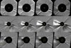 |
Fig. 1. Composite figure showing the arrival of the comet as seen in the VL by the Metis coronagraph on board Solar Orbiter (top row, on 24 December 20:46 UT and 25 December 00:22, 02:46, and 04:22 UT), by the COR2 coronagraph on board STEREO-A (middle row, on 25 December at 00:23, 02:23, 04:23, and 06:23 UT), and by the LASCO-C2 coronagraph on board SOHO (bottom row, on 25 December at 05:24, 06:24, 07:24, and 08:24 UT). In each panel the location of the comet is indicated by a yellow arrow; the yellow grid shows the Stonyhurst coordinates on the solar disk and the dark grid on the corona shows different latitudes (with steps of 15 deg) and altitudes (with steps of 1 R⊙). Each panel is obtained with JHelioviewer (Müller et al. 2017) as a base difference after the subtraction of the last available frame before the arrival of the comet in the instrument FoV. |
VL observations.
The earliest observation of the comet was 23 December 2021 19:06 UT in the SOHO/LASCO-C3 instrument. LASCO provides a continuous view of the Sun from its vantage at the Earth–Sun L1 Lagrange point via its two currently operating white-light coronagraphs, C2 and C3, each having an annular field of view (FoV) centered on the Sun (Brueckner et al. 1995). The outer coronagraph (C3) acquired approximately five ∼18 s “clear” filter (400–850 nm) full resolution (1024 × 1024 pixels) images per hour, and the inner coronagraph (C2) acquired approximately five ∼25 s “orange” filter (540–640 nm) full resolution images per hour (Fig. 1, bottom row). In total, the comet was observed in 111 C3 observations (23 December 2021 19:06 UT through 24 December 2021 23:42 UT) and 29 C2 observations (24 December 2021 03:12 UT through 08:48 UT), though it should be noted that the comet was partly or entirely obscured by the C3 occulter pylon (internal telescope structure) after approximately 24 December 2021 21:42 UT. It was also captured in a very small number of routine half-resolution color filter calibration observations made by LASCO-C3. However, due to the very limited availability of these images, we do not consider the color filter observations further.
The comet next appeared in STEREO-A’s white-light outer coronagraph, COR2, on 24 December 2021 11:53 UT (Fig. 1, middle row); concurrent observations were obtained with LASCO-C3 until the comet left the C3 FoV at 23:42 UT. STEREO-A follows a heliocentric orbit with a slightly smaller semimajor axis than Earth’s (Kaiser 2005). Since its launch in 2006, it has drifted ∼22.5° yr−1 ahead of Earth and had nearly caught up to Earth from behind at the time of observations (see Fig. 2). COR2 has an annular FoV (Howard et al. 2008) spanning 0.5°–4.0° at 14.7 arcsec pixel−1 resolution (2048 × 2048 nominal pixel resolution) with a fixed 650–750 nm bandpass (i.e., no other filters). COR2 records observations as both individually polarized image sequences (0° , ± 60°) and onboard summed total brightness images. The comet was observed in 57 COR2 observations until 25 December 2021 06:38 UT, with observations concurrent with LASCO-C2 beginning at 03:23 UT.
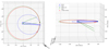 |
Fig. 2. Spacecraft constellation at time of perihelion, 25 December 2021 10:16 UT, as seen from above the ecliptic plane (left) and from a side view (right) in the Heliocentric Aries Ecliptic (HAE) reference system. Solar Orbiter’s orbit is shown in blue, and that of the Earth in green. At the time of the observations, the Sun–Solar Orbiter line was separated from the Sun–Earth line by only 9.4° and the spacecraft was at a distance of 1.01 AU from the Sun. STEREO-A (red) was 0.96 AU from the Sun, and separated from Solar Orbiter by almost 25°. SOHO, situated at the L1 point, can be assumed to be at the same location as Earth (green dot). The comet trajectory is shown, together with the FoV provided by the Metis coronagraph (blue triangles). |
The third telescope to detect the comet was Metis on board Solar Orbiter (Fig. 1, top row). At the time of the present observations the spacecraft was close to its aphelion at ≈1.01 AU and was at an angle of ∼9.2° eastward from the Earth–Sun line (see Fig. 2). Metis has an annular FoV approximately ranging between 1.9° and 3.4° from Sun’s center (Fineschi et al. 2020), corresponding in this case to a range of heights between 6.1 and 12.9 R⊙ in the corona, given the spacecraft’s heliocentric distance. The VL channel of the instrument can perform polarization observations acquiring sequences of images at four different orientations of the linear polarizer (a liquid-crystal variable retarder) in the bandpass 580–640 nm, and thus providing the possibility of measuring both the total and the linearly polarized components of the coronal VL brightness. On 24–25 December 2021, in particular, Metis was running a synoptic program alternating with calibration measurements. The synoptic observations used for this analysis consist of sequences of four polarization images with a total exposure time of 150 s (each image obtained by averaging on board five frames with exposure times of 30 s each), acquired with a cadence of 720 s (i.e., a full sequence of four images every 12 min). The VL detector, which has a nominal plate scale of 10.14 arcsec pixel−1, was configured with a 2 × 2 pixel binning, corresponding to a spatial resolution on the plane of the sky of ≈15 000 km bin−1. Since the interspersed calibration observations, lasting about one hour each, were repeated every four hours, the synoptic observations do not provide continuous coverage in that period, but have several gaps.
2.2. Photometry
Image processing and photometric measurements followed the standard procedures described in Knight et al. (2010) and Knight & Battams (2014), with a modification for the background removal that is described below. Publicly available level-0.5 LASCO images were calibrated using the SolarSoft IDL package (SSW; Freeland & Handy 1998). Background images were constructed by median combining 12 hr blocks of data with the same instrument, filter, and exposure time configuration. The same background was used for all images in the 12 hr block; the comet’s motion was fast enough that it was not detectable in the median, and thus had no effect on the photometry. The photometry was conducted by using a 2D Gaussian to determine the centroid, then measuring the flux in circular apertures of radius 350 arcsec for HI1, 224 arcsec for C3, and 71 arcsec for C2. The fluxes were converted to magnitudes using standard conversions.
The SOHO photometry is plotted in Fig. 3. The comet was first detected near the outer parts of C3 at the detection limit (nominal limiting magnitude is V ∼ 8.5), and brightened steadily until it was hidden by the C3 occulter pylon, when it had an apparent magnitude of V ∼ 4.5. A very short faint tail was visible in C3 in the few hours before this, and a clear very thin tail of about 0.5° in length when it reappeared in C2. At this time the comet magnitude was V ∼ 4.0; it faded rapidly, reached a minimum, and then had a slight increase in brightness again before entirely fading out of visibility. This brightening behavior is consistent with the lightcurves of comparably bright Kreutz comets (Knight et al. 2010). Although the clear (C3) and orange (C2) filter bandpasses do not overlap, extrapolation of the last C3 data to the first C2 data by assuming that the comet follows typical Kreutz photometric behavior and peaks around 10–15 R⊙ suggests that the orange filter data would have been about a magnitude brighter than the clear filter at the same heliocentric distance, which is typical for Kreutz comets.
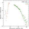 |
Fig. 3. Apparent magnitude of comet SOHO-4341 as a function of heliocentric distance in images from SOHO/LASCO-C3 (green circles) and LASCO-C2 (orange triangles). |
We estimated the comet’s radius to be ∼10 m by following the methodology used in Knight et al. (2010). We assumed that all of the light seen in C3 images is due to sunlight scattered by dust having an albedo of 0.04. We converted the apparent magnitude of each image to a cross section of dust using Eq. (4) in Jewitt (1991), where the phase angle correction uses the Schleicher-Marcus function (Schleicher & Bair 2011). We then assumed that all the dust particles are spherical grains of radius 1 μm to determine the number of grains, and then determine the effective radius these grains would have if they were assembled into a sphere. Since this model assumes that the radius has completely disintegrated at the time of maximum cross section, it is effectively a lower limit on the nucleus radius since any remaining solid nucleus is ignored. Our assumption ignores any contribution to the light from sodium emission; for a typical Kreutz comet, including this contribution would decrease the radius estimate by ∼20%. Other assumptions such as albedo, grain size, grain shape, particle size distribution, grain lifetimes, and dust-to-gas ratio could affect the result in either direction, so we caution that this size estimate is probably only accurate to within a factor of 2. Although this estimate is intended to give a time-varying nucleus size, we note that it yielded similar radius estimates from 11:00 UT to 23:00 UT on 21 December 2021, with earlier and later times yielding smaller values.
2.3. Orbit reconstruction
Along with photometric data, 140 astrometric measurements from the SOHO images, 57 from STEREO, and 40 from Metis images were extracted. Of the SOHO images, 111 were from C3 and 29 from C2. This was our first (and so far only) instance of measuring comet astrometry from Metis images. About 4000 comets have been measured from SOHO images and many from STEREO-A images. Their astrometric properties have been well determined, and the astrometric procedures employed for LASCO and COR2 observations have been continuously refined over the more than 25 years of the Sungrazer Project, and found to return astrometric uncertainties mostly at the sub-pixel level. We were able to assign astrometric uncertainties for the SOHO and STEREO-A observations as a function of magnitude, and then an orbit to those observations with the least-squares method with good results. SOHO and STEREO-A observed the comet SOHO-4341 with viewing angles that differed by about 35.4 deg. This large angle contributed parallax that resolved the ambiguities that often result from having data from only one spacecraft, and compensates somewhat for the relatively poor spatial resolution of the instruments.
Initially, a full six-parameter orbit was fit with no assumptions about the nature of the orbit. It proved sufficiently close to a parabolic orbit (eccentricity equal to one) to merit the usual practice of adding the e = 1 constraint, reducing the number of free parameters from six to five. This did not result in a significant change in the orbit, and the orbital elements from the full six-parameter solution are shown in Table 2. This orbit, fit solely to the STEREO-A and SOHO data, showed residuals of approximately 15″ for the Metis astrometry. Metis appears to be a promising source for astrometry, though this should be tested with further examples of this sort (objects whose astrometric data can be compared with that of known reliable sources).
Orbital elements of comet SOHO-4341 calculated from 237 observations (Heliocentric J2000 ecliptic elements; Epoch 2021 Dec 25.0 TT = JDT 2459573.5).
2.4. Tail 3D reconstruction
The observability of the comet from different viewpoints allowed us to carry out a 3D geometric reconstruction. This aspect is relevant for understanding the evolution of the VL tail (which is mainly composed of dust particles) and its “true” direction in space, and for determining any differences with the tail observed at other wavelengths (e.g., in UV with the hydrogen Ly-α line; see Sect. 3).
The spacecraft constellation available at the time of observations is shown in Fig. 2. We performed geometric triangulation of the VL tail by using images from STEREO-A/COR2 and Solar Orbiter/Metis-VL. Data from SOHO/LASCO-C2 could also be used (the separation angle is about 9 deg), but here we restricted our analysis to COR2-A and Metis-VL.
Total brightness images of the outer solar corona from Metis were obtained from the combination of the four images acquired at the four (effective) polarization angles of 49.1°, 84.3°, 133.2°, and 181.8°, by using the inverse of the Müller matrix measured during laboratory calibrations to derive images of the Stokes parameters I, Q, and U of the coronal VL (Capobianco et al. 2018; Casti et al. 2019; Liberatore et al. 2023). According to the theory of polarization, the total coronal brightness (tB) is then given by the Stokes parameter I, while the linearly polarized component (the polarized brightness, pB) is given by
 (1)
(1)
The standard calibration of Metis images includes the correction of detector bias and dark current, correction of detector flat field, correction of the optical vignetting function, and radiometric calibration of the data in units of the mean solar brightness (MSB) measured in the Metis VL bandpass. Since the acquisition of all the frames that were averaged to obtain the four images of a polarization sequence takes approximately ten minutes, the effective exposure time of the single total brightness (or tB) image derived from each sequence is ten minutes. This implies that moving objects like the observed sungrazing comet appear blurred or broadened in the images if their speed is such that their position projected on the plane of the sky varies more than one bin during the exposure time.
Total brightness images from COR2-A are constructed from triplets of single polarization images taken at 0°, 120°, and 240°. Double polarization images (i.e., taken at two different polarization angles, 0° and 90°) are also available within the time interval of the observation, but here we restricted the analysis to polarization triplets. COR2-A data are distributed as level 0.5 FITS files. Triplets of STEREO-A/COR1 FITS files were calibrated using the standard secchi_prep.pro routine part of SSW. The resulting COR2-A images are in DN/s units.
We removed the background from the calibrated data by using the scc_getbkgimg function and subtracting the resulting background image to the data and converted into MSB units by applying the conversion factor2
 (2)
(2)
We performed this conversion in order to have comparable values of the total brightness from both Metis and COR2-A.
We found six pairs of quasi-simultaneous observations (identified by a progressive number in the first column), which are separated in time by 1 min and 48 s. A big difference in the data is found in the acquisition time of the total brightness images. The acquisition time for Metis is around 10.2 min, as already said, while for COR2-A it is 1.1 min. The comet in the Metis images appears blurred because of the long acquisition time and the rapid motion of the object, reducing the actual spatial resolution in the VL images. The two spacecraft are not located at the same distance from the Sun (Solar Orbiter is farther than STEREO-A from the Sun), and the difference in the distance amounts to about 25 light seconds. Considering the large gap in the acquisition time, we disregard any correction in the light-travel time.
2.4.1. Geometric triangulation
After selecting the six pairs of near-simultaneous images, we proceeded with geometric triangulation with the widget tool scc_measure.pro, which is available in SSW. It requires as input the image arrays and the headers of the FITS files.
Figure 4 shows two screenshots of the scc_measure.pro tool. The COR2-A view is given in the left panels, while that from Metis is on the right. In order to highlight the comet tail, we gave as input the base difference image arrays, created by subtracting a frame acquired a few minutes earlier.
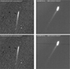 |
Fig. 4. Two examples (top and bottom) of graphical outputs of the scc_measure.pro routine showing VL images from STEREO-A/COR2 (left panels) and Solar Orbiter/Metis (right panels). The two images have different sizes and spatial resolution: the STEREO-A/COR2 images have a size of 2048 × 2048 pixels with a spatial resolution of 14.7 arcsec pix−1, while the Metis images are binned to a size of 1024 × 1024 pixels with a resolution of 20.3 arcsec pix−1. |
The user can, via the cursor of the mouse, move in every single panel and can actively select a sequence of tie-points that sample the shape of the feature under study. By clicking on a point in one of the two FoVs, the LoS of the instrument is drawn in the other FoV. Then, this line can cross the structure under interest at a certain point that is selected by the user. Having the two points for each instrument FoV, the procedure triangulates them and computes the coordinates in 3D space, which are given as Stonyhurst spherical coordinates (i.e., longitude, latitude, and radial distance from the Sun’s center). These coordinates can then be easily converted into a Cartesian reference frame, the Heliocentric-Earth-EQuatorial (HEEQ) coordinate system, defined as follows:
-
the x-axis along the Sun–Earth line pointing toward the Sun;
-
the z-axis coinciding with the solar rotation axis;
-
the y-axis lying on the solar equatorial plane and pointing westward.
Figure 4 shows two examples of the procedure for determining a single 3D tie-point. In the top panels, for example, a point is manually selected with the mouse at the tip of the comet coma, as seen in the Metis FoV (black cross). The LoS of the Metis instrument is then drawn in the left panel where the COR2-A image is given. For that case, the Metis LoS does not cross the comet as seen in COR2-A. This is just an effect of the longer acquisition time of Metis with respect to COR2-A, as we discussed previously. Because of the motion of the comet, the coma appears quite blurred, more elongated along the direction of movement in Metis than in COR2-A. To avoid strong uncertainties in the location of the tie-points, we first selected the initial point in the COR2-A FoV, then we chose the second one in the Metis FoV guided by the drawn LoS. This case is given in the bottom panels, with the first point selected at the tip of the coma as seen from COR2-A (left) and the second one chosen from the LoS line in the Metis FoV, which crosses the comet. We proceeded in this way, moving along the comet tail and selecting as many tie-points as necessary. By doing this, we dealt with the comet tail as a 1D feature.
2.4.2. 3D geometric reconstruction
The 3D tie-points sampling the VL tail are shown in Fig. 5; the orbit of the comet is in the HEEQ coordinate system, shown as a continuous red line. The comet orbit was traced by using the orbital parameters given in Table 2. The locations of the 3D tie-points are overplotted in Fig. 5 with different colors for each data set. The first data point of each set of 3D points almost lies on the trajectory. When we triangulated, we always pointed first at the comet coma, and then moved along the tail path.
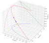 |
Fig. 5. Three-dimensional trajectory of the comet in the HEEQ reference frame (red line). The locations of the 3D points sampling the tail in the different sets of image pairs are shown as small colored dots. The different colors represent the different data sets at different times (see Table 3). The projections of the comet’s orbit onto the XY (blue), YZ (magenta), and XZ (green) planes are shown as dashed lines. The Sun’s position is shown as an orange dot, and its projections onto the different planes as colored dots. |
It is interesting to investigate the direction of the VL tail in 3D space. Table 3 reports a summary of the analysis of the 3D points for the tail, which are plotted in Figs. 6 and 7. In these figures, we show the different plane projections of the HEEQ coordinate system, namely the xy-plane (left panels), the yz-plane (middle panels), and the xz-plane (right panels). Each row refers to a specific data set which is identified by an ID number (which is also given in the first column of Table 3). The dashed red line represents the comet orbit path, while the 3D tie-points determined with the procedure scc_measure.pro are given as blue dots. When studying the direction of the tail in 3D space, the tie-points should be referred to the position of the comet nucleus along the orbit. This position is computed by taking into account the light-travel time from the comet to the observers. In principle, this would be different for the two observers. We avoided any complications, and for simplicity, since the sungrazing comet is very close to the Sun compared to the distance of 1 AU where the observers are located, we considered a light-travel time Δtlight = 8.3 min. Subtracting it from the observation times given in Table 3 (we considered the observation times from STEREO-A because of the shorter acquisition time), we then defined a reference time (Col. 4 of Table 3). Given this time, we determined the location of the comet nucleus r (in units of solar radii) and its instantaneous velocity v (in units of km s−1) in the HEEQ reference frame. The location of the comet nucleus is plotted in Figs. 6 and 7 as a green cross. The outward radial direction  with respect to the position of the comet is determined as
 (3)
(3)
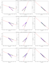 |
Fig. 6. Distribution of 3D tie points sampling the VL comet tail for the data sets listed in Table 3 (IDs 1-4). The three panels in each row show the projections of the tie points on the xy (left), yz (middle), and xz (right) planes of the HEEQ coordinate system. The points are plotted as blue dots. Shown relative to the position of the comet nucleus (green cross, as determined from the orbit) are the outward radial direction from the Sun (green arrow), the computed direction of the tail (magenta arrow), and the tangent to the comet trajectory (black arrow). The direction of the tail changes with respect to the radial and tangential direction along the comet orbit. The values of these angles are given above each sequence of panels. |
Summary of the analysis of each data set of 3D tie-points, identified by an ID number in the first column.
The tangent to the trajectory  at the comet position is found by using the velocity vector as
 (4)
(4)
The tail direction of the comet  is found as the vector that from the comet position r = (x, y, z) points to the barycenter of the 3D tie points distribution b = (xB, yB, zB), and hence
 (5)
(5)
Finally, the angles θr between  and
and  , and ϕt between
  and
and  are simply obtained as
 (6)
(6)
 (7)
(7)
The unit vectors  , and
, and  are shown as arrows in green, magenta, and black, respectively. The values of the angles θr and ϕt are reported in the title of each panel, and are also listed in Table 3. Considering the set of analyzed image pairs, the comet moves from a distance of about 15 R⊙ to about 8 R⊙. During this interval, the VL tail seems to depart from the radial direction: the angle θr increases from 3 deg to about 13 deg. On the contrary, the angle ϕt decreases at a lower rate from about 21 deg to 15 deg.
With the above 3D shape of the tail, we checked whether the tail lies in the plane defined by the comet trajectory and the radial vector from the Sun since in this case there are no forces outside that plane ( ). Figure 8 shows the distributions of the 3D points in the reference frame of the comet orbital plane; the axes are labeled Xorb, Yorb, and Zorb, with
  . The data points extend from the trajectories along a curve in the orbital plane of the comet (left panel) for distances on the order of one solar radius, while they are dispersed in the direction perpendicular to it (middle and right panels) in a spatial interval between approximately −0.02 and 0.04 R⊙. This dispersion is a measure of the uncertainty associated with the manual sampling of the tail. Our results show (within the uncertainties) that no significant deviations from the above-mentioned plane are observed.
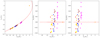 |
Fig. 8. Distributions of 3D tie-points sampling the VL comet tail in the reference frame of the comet trajectory: Xorb − Yorb coincides with the comet orbital plane; Zorb is perpendicular to it. The points tends to distribute along a curve lying in the orbital plane (left panel), while in the Zorb direction, the points are dispersed at most within ±0.04 R⊙. |
Furthermore, the tail observed in VL seems to be of dust origin, which follows a typical syndyne curve. The shape of such a curve is determined by the ratio of the radiation pressure force acting on a dust grain to the gravitational force that pulls the grain toward the Sun, which is then quantified by a parameter called β = Frad/Fgrav = CQpr/ρda (see, e.g., Kramer et al. 2014). The term C is a constant (C = 5.76 × 10⁻⁵ g cm−2), Qpr measures the scattering efficiency of dust and can be taken as equal to unity, ρd and a are respectively the density of dust grains and their typical size.
Figure 9 shows some attempts of fitting the 3D tie-points sampling the tail (for the data set IDs 3 and 6) with different values of β = 0.25, 0.50, 0.75, and 0.95. A larger deviation in the curves is found at the beginning of the tail in the coma, certainly due to an imperfect setting of the injection time for dust particles. We considered as reference times those listed in the Col. 4 of Table 3. On the other hand, dust particles can change their size in time because of erosion after emission from the coma. As a consequence, different segments of the VL tails could lie on syndynes with different β. This effect seems to be present in the tail from the data set 6 (Fig. 9, right), but more robust analysis would be required to prove such a scenario. In general, we find that the theoretical syndyne curves are very close to the determined data points. Assuming a value for the dust density of ρd = 1 g cm−3, the typical dust size a for values of β between 0.25 and 0.95 would be in the range of 6.1 × 10⁻⁵ − 2.3 × 10⁻⁴ cm.
 |
Fig. 9. Set of syndyne curves in different colors and styles for β = 0.25, 0.50, 0.75, 0.95 plotted against the sample data points tracking the VL comet tail in the orbital plane of the comet. The orbit of the comet is given by the dashed red line. |
2.5. Filtering of Metis VL observations
The total brightness images of Metis VL channel corresponding to Stokes I were processed using the Simple Radial Gradient Filter (SiRGraF: Patel et al. 2022). A total of 136 frames were used during the period from 24 December 2021 at 00:05 UT to 25 December 2021 at 22:41 UT to create the required minimum and uniform intensity backgrounds when filtering individual images with SiRGraF. This filtered out nearly constant background from the individual images. Since the background was created with observations acquired in short time intervals, short timescale dynamic structures such as CMEs and variable streamers were observed along with the comet under consideration. The left panel in Fig. 10 shows the comet along with other coronal structures after the application of SiRGraF. The propagation of the comet is shown via a zoomed-in view of the white dashed box in the same image.
 |
Fig. 10. Propagation of the sungrazer comet in the Metis VL FoV. In the left panel the location of the comet is shown in the dashed white box. A zoomed-in time sequence of the comet is shown in the six panels on the right. The starting time of the zoomed-in images is 2021-12-24 at 21:41 UT, followed by the five frames taken on 2021-12-25. |
3. Solar Orbiter observations in UV
3.1. Description of available UV data
In the Metis UV channel the comet was observed in 79 images acquired between 20:09 UT and 22:46 UT on 24 December. The images were acquired with an exposure time of 60 s and a cadence of 2 min, with an angular resolution of 81.6 arcsec bin−1 over 256 × 256 bins. Hence, the UV images were acquired with a higher cadence with respect to the VL images, and a lower spatial resolution. Considering the spacecraft distance from the Sun of 1.01 AU, this angular resolution corresponds to approximately 5.977 × 10⁴ km bin−1 projected on the Metis plane of the sky. Between 22:46 and 00:05 UT there was a gap in the UV data, and starting from the first UV image available on 25 December at 00:05 UT the comet was no longer visible, most likely because it was too faint with respect to the image noise level. As mentioned, the 3D reconstruction of the comet trajectory leads us to conclude that the comet was located in front of the Metis plane of the sky, and hence closer to Solar Orbiter than to the Sun. In particular, during the above observation interval the comet was on average at a heliocentric distance of 14.3 R⊙, and was moving at a velocity of 1663 km s−1 (1553 km s−1 in the radial direction to the Sun).
A magnification around the location of the comet in the full sequence of UV images acquired during the above time interval is shown in Fig. 11. In this sequence the comet enters near the southeast quadrant in the Metis images, and then moves mostly northward in the subsequent images. The images shown in Fig. 11 were obtained after the subtraction of an average UV background image, built with the last 12 UV images available before the comet arrival, and selected in the time intervals between 18:05 and 18:51 UT, and between 20:05 and 20:09 UT on 24 December.
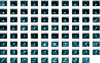 |
Fig. 11. Sequence of 79 UV images acquired on 24 December between 20:09:30 UT (top left) and 22:45:30 UT (bottom right). Each image shows a zoom-in over the detector region (located near the southeast corner) where the comet was observed; each zoomed-in region is 30 × 30 bins, corresponding to 40.8 × 40.8 arcmin. |
The sequence in Fig. 11 clearly shows, even after the subtraction of the background corona, that the UV frames were very noisy, making the comet emission barely distinguishable. Hence, a determination of the physical parameters of coronal plasma crossed by the comet in each single frame was not possible. In order to improve the signal-to-noise ratio, averaging over different images was required. The averaging procedure is explained in the next subsection.
3.2. UV images coalignment
Because the comet position was changing frame by frame, the averaging between different UV images necessarily required the coalignment of different images to the same location of the comet nucleus at different times. This procedure was needed even though, as mentioned above, the UV images were acquired at a much lower spatial resolution and a higher cadence with respect to the VL images. In the VL images acquired with a binning by 20.276 arcsec bin−1 the comet appears to move by about ten image bins between two subsequent pB images, having a time cadence of 12 min. Considering that the UV images were acquired with a spatial binning of 81.60 arcsec bin−1 and a cadence of 2 min, the above comet motion in the VL was expected to correspond in the UV to approximately 0.41 bins from one exposure to the subsequent one. Hence, to average over ten UV images it was necessary to compensate for motion by up to 4.1 bins.
By assuming that from one frame to the subsequent one the projected comet speed is approximately constant, the comet positions measured at different times from the VL were thus interpolated and resampled to the UV observation times and spatial resolutions. In this way it was possible to determine, for each sequence of ten UV images, the corresponding fractional shifts over the two coordinates Δx and Δy to be applied to co-align the images to the same position of the comet. After the image coalignment, the available 79 images were averaged over ten elements, thus corresponding to the average Lyman-α emission observed over about 20 min.
The resulting eight average images are shown in Fig. 12, again after the subtraction of the average Lyman-α coronal background image. Each image is the result of coalignment and averaging of the images shown in each row in Fig. 11. These images show a clear improvement in the signal-to-noise ratio; the Lyman-α tail of the comet is clearly visible in all images. Nevertheless, for the purposes of the research described here (see next paragraph for details), it turned out that even these average images did not have the quality required to measure the variations over time of the Lyman-α tail distribution properties, and in particular the tail length, width, and inclination with respect to the anti-solar direction. The easiest parameter to be determined from these eight images was the Lyman-α tail length (see next paragraph), which provided an estimate of the local electron density at different times and altitudes in the solar corona, but the values resulting at different altitudes were (within the error bars) almost constant in a range of heliocentric distances going from 13 to 15 R⊙.
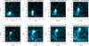 |
Fig. 12. Sequence of eight UV images obtained on December 24 between 20:09:30 UT (top left) and 22:45:30 UT (bottom right) after co-alignment and averaging over ten subsequent images. Each image shows a zoom-in over the detector region (located near the southeast corner) where the comet was observed; each zoomed-in region is 30 × 30 bins, corresponding to 40.8 × 40.8 arcmin. |
Hence, for the detailed scientific analysis we focus on the average UV image obtained after the co-alignment and averaging over the whole number of available 79 UV images. The resulting average UV image is shown in Fig. 13, representative of the comet appearance at an average heliocentric distance of 14.3 R⊙. In this figure the vertical stripes are an artifact created by the co-alignment of the different Metis coronagraphic images to the same locations of the comet nucleus as a function of time. The average Lyman-α comet image is clearly visible in the southeast corner of the image (see Fig. 14 for a zoomed-in version of this figure). The position of the solar disk is overplotted at the coordinates corresponding to the intermediate time between the starting acquisition time of the first exposure and the ending acquisition time of the last exposure.
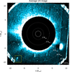 |
Fig. 13. Average Lyman-α image resulting after the co-alignment and averaging of all 79 images acquired on 24 December 2021 between 20:09:30 UT and 22:45:30 UT. The position of the comet is indicated by the yellow box. |
3.3. UV images analysis
As briefly described by Bemporad et al. (2015), the 2D distribution of the Lyman-α emission due to a sungrazing comet can be analyzed to derive at least three physical parameters of the local coronal plasma crossed by the comet: the electron density ne, the solar wind speed vwind, and the proton kinetic temperature Tk. The determination of these parameters for the plasma crossed by SOHO-4341 is described here.
As first pointed out by Uzzo et al. (2001) and then also exploited by other authors (Bemporad et al. 2005; Giordano et al. 2015), for sungrazing comets the local plasma density ne can be derived from the tail extension Ltail along the main axis of the tail. The observed Lyman-α emission could in principle be due to three different generations of H atoms (see Raymond & Giordano 2019): the first-generation neutrals H1, due to the dissociation of water molecules outgassed by the cometary nucleus; the second-generation neutrals H2, due to the charge exchange between H1 and solar wind protons; and the third-generation neutrals H3, produced by further charge transfer between the H1 and H2 atoms, and the pick-up ions produced by the ionization of the H1 atoms.
The main difference between these three generations of neutrals is the corresponding velocity distribution: H1 atoms are almost traveling with the cometary nucleus because the velocity v0 imparted by the cometary outgassing and water dissociation is negligible (lower than 30 km s−1; see, e.g., Shimizu 1991) with respect to the cometary speed vcom (on the order of 160 − 170 km s−1 for this comet during the acquisition of UV images; see Table 3). On the contrary, H2 atoms are moving mostly with the solar wind speed distribution vwind because the momentum transfer in the charge exchange process between H atoms and protons is almost negligible (McClure 1966). Finally, the H3 atoms move parallel to the local magnetic field with the corresponding projected component v// of the solar wind speed (Raymond & Giordano 2019).
The H1 atoms travel only a distance on the order of dH1 ≃ v0τH before undergoing ionization or charge transfer. Their lifetime τH (neglecting other second-order processes) can be estimated as (see, e.g., Uzzo et al. 2001)
 (8)
(8)
where τcx is the time required for charge exchange between cometary neutrals and coronal protons, and τion = 1/(1/τphot + 1/τcoll) is the time for ionization by coronal electrons (mainly due to photo-ionization and collisional ionization occurring at times τphot and τcoll, respectively). As a first estimate (which is refined below), these times are on the order of τion ∼ τcx ∼ 3.1 × 107 cm−3 s/ne (Uzzo et al. 2001; Bemporad et al. 2005), and by assuming an electron density on the order of ne ∼ 104 cm−3 at the heliocentric distance of 14 R⊙ (see, e.g., Lamy et al. 2021), this corresponds to τH ≃ 1.55 × 10³ s, and hence, by assuming for instance v0 ≃ 15 km s−1, it turns out that dH1 ≃ 2.32 × 10⁴ km, which corresponds to about 0.5 bin in the UV images. Hence, any emission from these atoms is located only in the proximity of the cometary nucleus location. Moreover, since these H1 atoms are mostly traveling with the comet nucleus, and hence at a radial speed of about 155 km s−1, their Lyman-α emission (almost entirely due to the resonant scattering process) is reduced by the “Swings-effect” (Bemporad et al. 2007) by a factor of about 0.6–0.7 (see, e.g., Fig. 1 in Bemporad et al. 2021).
On the other hand, the H2 atoms travel at a speed vrel relative to the cometary nucleus given by
 (9)
(9)
where vrcom and vtcom are respectively the radial and tangential components of the cometary speed, and vwind is the solar wind speed (assumed to be radial at these heliocentric distances). The number of H2 atoms, and thus the observed Lyman-α emission along the tail, exponentially decay as exp( − t/τion), and hence by measuring the distance Ltail at which the Lyman-α emission is reduced by a factor of 1/e, it is possible to directly measure the time τion = Ltail/vrel.
Nevertheless, because the cometary speed components are known but the local solar wind speed is unknown, this measurement requires vwind to be determined or assumed first. Previous works, mostly based on SOHO/UVCS observations, applied this technique to measure the local coronal density by assuming a value for the local solar wind speed (see, e.g., Uzzo et al. 2001; Bemporad et al. 2005; Giordano et al. 2015), and this measurement was unsuccessfully attempted with SOHO/UVCS only by Bemporad et al. (2007), based on the images reconstructed from spectroscopic observations. On the contrary, in this work, thanks to the availability of a 2D image of the Lyman-α emission provided for the first time by the Metis coronagraph, it is possible to measure the local solar wind speed. In particular, as described by Bemporad et al. (2015), the solar wind speed can be measured from the tail inclination angle εcom with respect to the cometary orbital path direction. The second-generation neutrals H2 are deposited along the cometary orbital path, but then propagate outward at the solar wind speed. Hence, the slower (the faster) the local wind speed met by the comet, the more the Lyman-α tail will be aligned with the cometary orbital path (with the anti-solar radial direction).
A zoomed-in image of the average Lyman-α emission (after subtraction of the average coronal background) is provided in Fig. 14, showing the derived orientation of the Lyman-α tail (red line) with respect to the anti-solar radial direction (yellow line), and the cometary orbital path (orange line). The predominant tail orientation was determined first by fitting with Gaussian profiles of the Lyman-α intensity distributions across the tail observed in each row of the 2D image, as shown in Fig. 15. Hence, the resulting different locations of the peaks along the tail have been further analyzed with a linear fitting, as shown in the left panel of Fig. 16. This figure shows the location of the Gaussian centroids along the tail, plotted starting from the location of the Lyman-α emission peak. The derived Lyman-α tail inclination is the same as shown with a red line in Fig. 14. The resulting measured value (after subtraction of the comet’s orbital inclination shown with an orange line in Fig. 14) is εcom = 9.7 ± 1.6 deg.
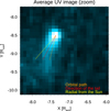 |
Fig. 14. Magnified image of the comet Lyman-α emission corresponding to the area surrounded by the yellow box in Fig. 13 and resulting after averaging between 20:09:30 UT and 22:45:30 UT on 24 December 2021. The coronal average background emission has been subtracted. |
Given the value of εcom, it is possible to measure the local solar wind speed vwind (assumed to be radial), given the radial (vrcom) and tangential (vtcom) cometary velocities, as
 (10)
(10)
with vrcom = 155 km s−1 and vtcom = 59 km s−1 it turns out that vwind = (190 ± 50) km s−1. With the above value of the solar wind speed, the speed of H2 atoms relative to the cometary nucleus is vrel = (350 ± 50) km s−1, and with the measured value of the Lyman-α tail length Ltail = (6.5 ± 0.7)×105 km, it is τion = Ltail/vrel = (2100 ± 400) s. We note that the above value for the Lyman-α tail length was measured from the reconstructed location of the cometary nucleus and corrected also taking into account projection effects related to the fact that the comet was not moving on the Metis plane-of-sky (see Fig. 15), corresponding to the plane passing through the center of the Sun and perpendicular to the telescope LoS.
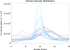 |
Fig. 15. Lyman-α intensity distribution across the cometary tail, going from the profile at the emission peak (light blue) to the profile at the end of the tail (dark blue). For each row the solid lines show the observed Lyman-α intensity, while the dotted lines show the corresponding Gaussian fits. Different colors in each curve correspond to different locations along the tail, going from the location of the comet nucleus (light blue) to the end of the tail (dark blue). |
Now, in order to derive the estimate of the local solar wind electron density ne from the above H2 atoms’ lifetime, it is necessary to estimate the time for the H2 atoms collisional ionization τcoll. Given τcoll, it is possible to directly estimate ne = 1/(τcollqcoll) with qcoll (cm3 s−1) collisional ionization rate coefficient, provided by Scholz & Walters (1991) for different plasma temperatures Tk. Considering only collisional and photoionization, the time τcoll is related to the measured τion simply by 1/τion = 1/τcoll + 1/τphot. The H atoms photoionization rate 1/τphot was recently measured at the heliocentric distance of 1 AU by Sokół et al. (2019) who provided 1/τphot ≃ 0.7 × 10⁻⁷ s−1 at 1 AU for the year 2018. By rescaling this rate as 1/r2 to the comet heliocentric distance of 14 R⊙, and by considering that at the end of 2021 the Lyman-α solar irradiance was comparable with the value measured by the Solar EUV Experiment (SEE; Woods et al. 2005) in 2018, it turns out that τphot = 6.0 × 10⁴ s, and hence τcoll ≃ τion = (2100 ± 400) s.
Now the kinetic temperature Tk is the only missing plasma parameter needed to have an estimate of qcoll (Scholz & Walters 1991), and finally to derive ne. In the previous analyses of sungrazing comets observed by the SOHO/UVCS spectrometer it was possible to directly measure Tk from the observed Lyman-α line profile width, but this measurement is not possible here with the Metis coronagraph. Nevertheless, as mentioned by Bemporad et al. (2015) and anticipated above, this plasma parameter can also be measured from the observed aperture angle of the Lyman-α tail (see also Raymond & Giordano 2019). It can be assumed that after the transit of the comet the second-generation neutrals H2 undergo a diffusion in the direction perpendicular to the main tail axis due to their kinetic temperature. Under this assumption, the tail semi-aperture angle αtail is related to the thermal speed  simply by
 (11)
(11)
The measurement of the αtail is shown in the right panel of Fig. 16 providing the widths of the Lyman-α distributions measured with Gaussian fits and the corresponding linear fit. From these measurements αtail = (24 ± 3) deg, hence vtherm = (140 ± 30) km s−1, and Tk = (1.2 ± 0.4)×106 K. For this plasma temperature the corresponding collisional ionization rate is qcoll = 3.22 × 10⁻⁸ cm3 s−1.
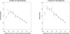 |
Fig. 16. Determination of solar wind speed and proton temperature from the analysis of the Lyman-α intensity distribution. Left: determination of the predominant tail orientation by linear fitting of the peak locations of Gaussian Lyman-α intensity distribution across the tail. Right: determination of the cometary Lyman-α tail semi-aperture angle. |
In this way it is possible finally to also derive the electron density ne that will be simply given by ne = 1/(τcollqcoll) = (1.5 ± 0.3)×104 cm−3. This value is in acceptable agreement (within the uncertainties) with those recently provided for instance by Lamy et al. (2021) from LASCO-C3 measurements in the equatorial plane (see their Fig. 42, middle panel), and hence for ambient coronal streamer conditions.
In summary, this showed how, from the analysis of the Lyman-α cometary tail 2D distribution, it was possible to measure at an average heliocentric distance of 14.3 R⊙ the solar wind speed (vwind = (190 ± 50) km s−1), the proton kinetic temperature (Tk = (1.2 ± 0.4)×106 K), and the electron density (ne = (1.5 ± 0.3)×104 cm−3). These measurements (which are discussed in the Conclusions) are independent of the radiometric calibration of the Lyman-α observations. On the other hand, the measurement of the cometary outgassing rate, and hence of the most likely cometary nucleus size, requires the use of images that are radiometrically calibrated. For this reason, before discussing the determination of cometary parameters, we describe in the next subsection how the radiometric calibration of the Lyman-α images was further tested.
3.4. UV images radiometric calibration
The accuracy of the UV radiometric calibration was verified by photometric measurements of the star Theta Ophiuchi, which crossed the Metis FoV in the days before the arrival of the comet. In this period the Metis instrument acquired UV images with exposure times of 60 s, but in these images Theta Ophiuchi was partially saturated, which affected the photometry. Hence, to avoid this issue, the calibration was verified by using only the level L2 data acquired with exposure times of 10 or 30 s. For each image, between 03:00 UT on 24 December and 15:00 UT on 25 December, a bi-Gaussian curve was fit over the 2D stellar emission distribution to derive its total flux and the extension of brightness distribution. In Fig. 17 we show the location of the star at five different times in the time interval between 23 and 25 December 2021 (see the exact times provided in the figure). This figure also shows the varying vignetting in the Metis instrument FoV as the star is observed closer to the inner occulter edge.
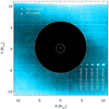 |
Fig. 17. Location of the star Theta Ophiuchi in the Metis UV images at five different times between 23 and 25 December 2021 (the exact times are shown in the figure). The inner circle shows the location of the solar disk behind the Metis coronagraph occulter, while the diamond and triangle correspond respectively to the center of the solar disk and the location of the Metis Internal Occulter (IO). |
The Metis level L2 data contain three different images in each FITS file: the actual intensity image, an image providing the errors associated with each pixel, and a validation matrix. From the errors associated with each pixel, it was possible to estimate the errors of the parameters derived by the bi-Gaussian fitting, and in particular the peak intensity value I*, and the 1/e widths of the bi-Gaussian in the direction of the image columns (σx) and rows (σy). The resulting star’s flux F* corresponds to the volume of the bi-Gaussian curve F* = 2π I*σx σy. The intensities in the Metis L2 images are provided pixel-by-pixel in units of phot cm−2 s−1 sr−1; considering that the images have 1024 × 1024 pixels and the binning level is 1 (with 1 bin = 20.4 arcsec), the pixels were converted to arcsec, and the value of the solid angle covered by 1 bin was then multiplied by the measured flux. By averaging over all the values derived from different exposures, the resulting value for the star’s flux is F* = 4.29 × 10⁴ phot cm−2 s−1.
The estimated value was compared, within the uncertainties, with the reference value. The reference value was obtained by integrating the convolution of the spectrum of the star Theta Ophiuchi with the spectral response of the filter and the detector of the UV channel. The Theta Ophiuchi spectrum is available in the International Ultraviolet Explorer (IUE) observations provided in the MAST archive (Willis 2013; Landsman & Simon 1993). This approach to obtain the reference value of the stellar flux is the same used to perform the in-flight radiometric calibration of the UV channel of Metis using stars, as explained in De Leo et al. (2023). The resulting reference value is F* = 4.75 × 10⁴ phot cm−2 s−1; this is in agreement (within ∼10%) with the value measured from the Metis images and provided above. Hence, the radiometric calibration of the exposures acquired during the transit of the comet can be also considered reliable within this uncertainty.
The 2D distribution of the stellar brightness in the images also provided an estimate of the Metis instrument spatial resolution in the detector region crossed by the star. By plotting σx and σy, in bins and in arcseconds, it showed that as one variable increased the other increased as well, but in a non-symmetrical way; this means that the telescope is affected by optical aberrations, so the point spread function of the telescope is not perfectly symmetric. The mean values obtained for these parameters are σx = 2.338 bin = 47.700 arcsec and σy = 2.650 bin = 54.050 arcsec.
3.5. UV light curve analysis
Under the assumption of isotropic outgassing from a spherical cometary nucleus with radius r0 (cm), the number density of neutral H atoms nH (cm−3) having a lifetime τH (s) can be written as a function of distance r (cm) from the nucleus as
 (12)
(12)
by neglecting the unknown time required by H2O molecules to be photo-dissociated, and by assuming an average outflow speed v0 of the neutrals with number density n0 (cm−3) at the nucleus surface. By integrating (assuming cylindrical symmetry) the above 3D distribution of H number density along the LoS, and also in the direction perpendicular to the projected cometary tail extension, the resulting number density nH1 (cm−1) of first-generation H atoms along the tail s can be written as
 (13)
(13)
and the above expression can be integrated numerically to derive the 1D symmetric distribution along the tail (coordinate s) of first-generation neutral H atoms, assuming that the cometary nucleus is located at the position s = 0. If the comet is moving radially with inward velocity vrcom (i.e., toward the Sun), and the solar wind is expanding outward also radially with velocity vwind, in stationary conditions the number of second-generation H atoms NH2(s) deposited in the corona by charge exchange between cometary neutrals and coronal protons can be written as
 (14)
(14)
The above expression assumes that the speed of H2 atoms reaches their asymptotic value close to the comet because the outflow speed of first-generation neutrals H1 is very small. Moreover, it assumes that the cometary neutrals are all moving toward the Sun at the same speed vrcom, a valid approximation considering that under normal conditions for sungrazing comets it is vrcom ≫ v0. Once the second-generation neutrals are formed, because the momentum transfer in the charge exchange process is negligible, the resulting H atoms have the same velocity distribution as the solar wind protons, and also diffuse with respect to the location in which they were deposited with the proton speed thermal velocity vth. Hence, the resulting distribution NUV of H atoms along the tail coordinate s responsible for the UV emission can be obtained by a convolution integral
![Mathematical equation: $$ \begin{aligned} N_{\rm UV}(s) =\frac{1}{\sqrt{\pi } \, v_{\rm th} \tau _{\rm ion}}\int _{-\infty }^{+\infty } \!\!\! N_{\rm H2}(s^{\prime }) \,\exp {\left[ - \frac{(s-s^{\prime })^2}{\Delta s_{\rm th}^2} \right]}\, \mathrm{d}s^{\prime } ,\end{aligned} $$](/articles/aa/full_html/2023/12/aa46881-23/aa46881-23-eq27.gif) (15)
(15)
where  is the profile broadening due to the proton thermal speed, and
  is the thermal speed of solar wind protons having a kinetic temperature Tk.
This total number of H atoms along the tail emitting the UV radiation needs to be converted into the number of expected Lyman-α photons in order to compare the theoretical curve with the observed intensity curve. In this work the UV Lyman-α intensity was computed by using the explicit expression provided by Bemporad et al. (2021) for the Lyman-α emission (Eq. (18) in that work), and by also using the analytic expression provided for the Doppler dimming coefficient (Eq. (17) in that work). The only part that needs to be modified in the above equations is the term relating the observed UV intensity to the LoS integration of the electron density ne, to consider that, different from the solar corona, the comet tail emission is limited along the LoS. In particular, by measuring the projected average tail width 2 dtail and by assuming in 3D a cylindrical shape with cross section area  , the expression for the Lyman-α emission provided by Eq. (18) in Bemporad et al. (2021) can be modified by simply replacing the quantity
![Mathematical equation: $$ \begin{aligned} 0.83 \, R_{\rm H}[T_{\rm e}(s)] \int _{-\infty }^{+\infty } n_{\rm e}(z) \, \mathrm{d}z, \end{aligned} $$](/articles/aa/full_html/2023/12/aa46881-23/aa46881-23-eq31.gif) (16)
(16)
representing the number of neutrals emitting the Lyman-α radiation along the LoS (with RH fraction of neutral hydrogen atoms depending on the electron temperature Te), with the quantity  , with NUV(s) given by the above Eq. (15).
Given the cometary orbital parameters, the solar wind plasma parameters measured above, and by assuming for H atoms (in agreement with Uzzo et al. 2001) a speed v0 = 15 km s−1 resulting from the combination of the outgassing speed from the comet nucleus near the Sun (see, e.g., Giordano et al. 2015) plus the speed from the photodissociation of H2O and OH molecules (e.g., van Dishoeck & Dalgarno 1984; Mancuso 2015), the above equations allow us to determine the cometary radius r0 better reproducing the total Lyman-α emission observed along the tail after integration in the direction perpendicular to the tail, considering that
 (17)
(17)
with QH2O the water molecule production rate from the comet nucleus, Acom = 0.06 the cometary albedo, F⊙ the solar radiation flux rescaled at the cometary heliocentric distance, NA Avogadro’s number, and LH2O the water latent heat for sublimation.
The input Lyman-α emission distribution along the tail and the resulting fitting curves are shown in Fig. 18, with solid and dotted lines respectively. The location of the cometary nucleus (not coincident with the location of the Lyman-α emission peak) was adjusted in order to optimize the coincidence between the observed and the reconstructed Lyman-α peaks. The resulting cometary radius turns out to be r0 = (65 ± 10) m, providing an outgassing rate QH2O = (4.8 ± 1.5)×1028 molec s−1. We note that these values were obtained here by assuming a single spherical active surface on the nucleus, but the same outgassing rate could also be produced by a greater number of smaller comet fragments with smaller total volume, but resulting in the same total active area. Considering that the fitted Lyman-α emission shown in Fig. 18 results from an average between images acquired between 20:09 and 22:45 UT on 24 December 2021, these values should be considered as average values in this time interval, when the comet was at an average heliocentric distance of 14.3 R⊙.
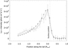 |
Fig. 18. Lyman-α intensity distribution along the cometary tail, plotted as a function of distance from the location of the emission peak. Because of the comet’s relative speed with respect to the solar wind, the location of the comet nucleus is shifted by about 0.1 R⊙ with respect to the location of the Lyman-α emission peak. |
4. Discussion and conclusions
Between 24 and 25 December 2021 the Metis coronagraph on board Solar Orbiter observed a sungrazing comet. This is the first ever reported sungrazing comet observed at the same time in the VL and UV band-pass images by a coronagraph. This object was observed by Metis at an average heliocentric distance by 14.3 R⊙, but the comet was at a distance of ∼7.9 R⊙ from the plane of the sky of the Metis observations. Hence, the coronagraphic images cannot provide any information to understand whether the comet was crossing a coronal region more typical of slow or fast solar wind. The same also applies to coronagraphic images acquired by SOHO and STEREO-A. As mentioned, because the main Lyman-α emission is due to second-generation neutrals traveling with the solar wind speed distribution, it is important to take into account that the observation of a Lyman-α tail is indicative of a local solar wind speed lower than ∼300 km s−1. For higher solar wind speed, the second-generation neutral H atoms would also have a higher radial speed, and hence their emission would be severely reduced by the Doppler dimming effect (see, e.g., Bemporad et al. 2021, and references therein).
On the other hand, it is also interesting to discuss why for this comet the UV Lyman-α emission fades before the VL emission. This is the opposite of what was reported for instance by Giordano et al. (2015) for sungrazing comet C/2002 S2. It is possible that the nucleus of the comet reported here disintegrates between 12 and 14 R⊙, but the stream of large dust particles continues inward, slowly sublimating as it goes. Sublimation times for 100 nm olivine dust grains at 12–14 R⊙ are around 1000 s (Kimura et al. 2002), but they are much longer for pyroxene. A dust tail without an apparent nucleus was observed after the breakup of comet C/2012 S1 (ISON) (Curdt et al. 2014). In addition, if the comet disintegrated, this could explain the larger radius estimated from the UV Lyman-α. Disintegration would greatly increase the cross-section of both reflecting dust and sublimating ice, but the ice would likely have a shorter lifetime than the time it takes the dust grains to leave the photometric aperture, thus producing a light curve fading more rapidly in UV than VL.
Near-simultaneous observations in VL between SolO/Metis and STEREO-A/COR2 allowed us to reconstruct in 3D the tail shape, which is well represented by a syndyne curve. This confirms the nature of the VL tail in terms of dust grains. A set of syndyne curves in the range of β = [0.25, 0.95] approximately fit the determined data points sampling the VL tail in 3D. Such values of β would be associated with dust grain size of a = [7.7 − 23]×10−5 cm for a typical value of dust density ρd = 1.0 g cm−3.
Thanks to the methods originally proposed by Bemporad et al. (2015), the analysis of the UV Lyman-α tail allowed us to estimate the main physical parameters of the coronal plasma crossed by the comet, confirming again (as also discussed for instance by Giordano et al. 2015) that these objects can be considered as local probes of the coronal plasma. Moreover, the analysis of the VL and UV emissions allowed us to estimate the equivalent radius of the dusty part (10 m) and icy part (65 m) of the comet. It is not simple to convert these numbers into an estimate of the dust-to-ice ratio, in particular because recent Rosetta observations demonstrate that the particles (at least at the surface of the nucleus) are rather “fluffy” (Güttler et al. 2019), with fractal dimensions of 1.5–2.5. Taking this fractal dimension into account, the ratio of the nucleus radii of the effective dusty to icy parts of the comet would probably be higher.
Acknowledgments
G. Nisticò acknowledges support from the “Rita Levi Montalcini 2017” fellowship funded by the Italian Ministry of Research. K.B. was supported by the NASA Sungrazer Project. Solar Orbiter is a space mission of international collaboration between ESA and NASA, operated by ESA. The Metis programme is supported by the Italian Space Agency (ASI) under the contracts to the co-financing National Institute of Astrophysics (INAF): Accordi ASI-INAF N. I-043-10-0 and Addendum N. I-013-12-0/1, Accordo ASI-INAF N.2018-30-HH.0 and under the contracts to the industrial partners OHB Italia SpA, Thales Alenia Space Italia SpA and ALTEC: ASI-TASI N. I-037-11-0 and ASI-ATI N. 2013-057-I.0. Metis was built with hardware contributions from Germany (Bundesministerium für Wirtschaft und Energie (BMWi) through the Deutsches Zentrum für Luft- und Raumfahrt e.V. (DLR)), from the Academy of Sciences of the Czech Republic (Czech PRODEX) and from ESA.
References
- Antonucci, E., Romoli, M., Andretta, V., et al. 2020, A&A, 642, A10 [NASA ADS] [CrossRef] [EDP Sciences] [Google Scholar]
- Battams, K., & Knight, M. M. 2017, Phil. Trans. R. Soc. London Ser. A, 375, 20160257 [Google Scholar]
- Bemporad, A., Poletto, G., Raymond, J. C., et al. 2005, ApJ, 620, 523 [NASA ADS] [CrossRef] [Google Scholar]
- Bemporad, A., Poletto, G., Raymond, J., & Giordano, S. 2007, Planet Space Sci., 55, 1021 [NASA ADS] [CrossRef] [Google Scholar]
- Bemporad, A., Giordano, S., Raymond, J. C., & Knight, M. M. 2015, Adv. Space Res., 56, 2288 [CrossRef] [Google Scholar]
- Bemporad, A., Giordano, S., Zangrilli, L., & Frassati, F. 2021, A&A, 654, A58 [NASA ADS] [CrossRef] [EDP Sciences] [Google Scholar]
- Biesecker, D. A., Lamy, P., & St Cyr, O. C., Llebaria, A., & Howard, R. A., 2002, Icarus, 157, 323 [NASA ADS] [CrossRef] [Google Scholar]
- Brueckner, G. E., Howard, R. A., Koomen, M. J., et al. 1995, Sol. Phys., 162, 357 [NASA ADS] [CrossRef] [Google Scholar]
- Capobianco, G., Casti, M., Fineschi, S., et al. 2018, in Space Telescopes and Instrumentation 2018: Optical, Infrared, and Millimeter Wave, eds. M. Lystrup, H. A. MacEwen, G. G. Fazio, et al., SPIE Conf. Ser., 10698, 1069830 [Google Scholar]
- Casti, M., Fineschi, S., Capobianco, G., et al. 2019, in International Conference on Space Optics— ICSO 2018, eds. Z. Sodnik, N. Karafolas, & B. Cugny, SPIE Conf. Ser., 11180, 111803C [Google Scholar]
- Curdt, W., Boehnhardt, H., Vincent, J. B., et al. 2014, A&A, 567, L1 [NASA ADS] [CrossRef] [EDP Sciences] [Google Scholar]
- De Leo, Y., Burtovoi, A., Teriaca, L., et al. 2023, A&A, 676, A45 (SO Nominal Mission Phase SI) [NASA ADS] [CrossRef] [EDP Sciences] [Google Scholar]
- Fineschi, S., Naletto, G., Romoli, M., et al. 2020, Exp. Astron., 49, 239 [Google Scholar]
- Freeland, S. L., & Handy, B. N. 1998, Sol. Phys., 182, 497 [Google Scholar]
- Giordano, S., Raymond, J. C., Lamy, P., Uzzo, M., & Dobrzycka, D. 2015, ApJ, 798, 47 [Google Scholar]
- Güttler, C., Mannel, T., Rotundi, A., et al. 2019, A&A, 630, A24 [NASA ADS] [CrossRef] [EDP Sciences] [Google Scholar]
- Howard, R. A., Moses, J. D., Vourlidas, A., et al. 2008, Space Sci. Rev., 136, 67 [NASA ADS] [CrossRef] [Google Scholar]
- Jewitt, D. 1991, in IAU Colloq. 116: Comets in the post-Halley era, eds. J. Newburn, R. L. M. Neugebauer, & J. Rahe, Astrophys. Space Sci. Lib., 167, 19 [NASA ADS] [Google Scholar]
- Jones, G. H., Knight, M. M., Battams, K., et al. 2018, Space Sci. Rev., 214, 20 [NASA ADS] [CrossRef] [Google Scholar]
- Kaiser, M. L. 2005, Adv. Space Res., 36, 1483 [NASA ADS] [CrossRef] [Google Scholar]
- Kimura, H., Mann, I., Biesecker, D. A., & Jessberger, E. K. 2002, Icarus, 159, 529 [NASA ADS] [CrossRef] [Google Scholar]
- Knight, M. M., & Battams, K. 2014, ApJ, 782, L37 [CrossRef] [Google Scholar]
- Knight, M. M., A’Hearn, M. F., Biesecker, D. A., et al. 2010, AJ, 139, 926 [Google Scholar]
- Kramer, E. A., Fernandez, Y. R., Lisse, C. M., Kelley, M. S. P., & Woodney, L. M. 2014, Icarus, 236, 136 [NASA ADS] [CrossRef] [Google Scholar]
- Lamy, P., Gilardy, H., Llebaria, A., Quémerais, E., & Ernandez, F. 2021, Sol. Phys., 296, 76 [NASA ADS] [CrossRef] [Google Scholar]
- Landsman, W., & Simon, T. 1993, ApJ, 408, 305 [CrossRef] [Google Scholar]
- Liberatore, A., Fineschi, S., Casti, M., et al. 2023, A&A, 672, A14 (SO Nominal Mission Phase SI) [NASA ADS] [CrossRef] [EDP Sciences] [Google Scholar]
- Mancuso, S. 2015, A&A, 578, L7 [NASA ADS] [CrossRef] [EDP Sciences] [Google Scholar]
- Marsden, B. G. 1989, AJ, 98, 2306 [NASA ADS] [CrossRef] [Google Scholar]
- Marsden, B. G. 2005, ARA&A, 43, 75 [Google Scholar]
- McClure, G. W. 1966, Phys. Rev., 148, 47 [NASA ADS] [CrossRef] [Google Scholar]
- Müller, D., Nicula, B., Felix, S., et al. 2017, A&A, 606, A10 [Google Scholar]
- Müller, D., St Cyr, O. C., Zouganelis, I., et al. 2020, A&A, 642, A1 [Google Scholar]
- Patel, R., Majumdar, S., Pant, V., & Banerjee, D. 2022, Sol. Phys., 297, 27 [NASA ADS] [CrossRef] [Google Scholar]
- Raymond, J. C., & Giordano, S. 2019, ApJ, 887, 45 [NASA ADS] [CrossRef] [Google Scholar]
- Raymond, J. C., Fineschi, S., Smith, P. L., et al. 1998, ApJ, 508, 410 [NASA ADS] [CrossRef] [Google Scholar]
- Raymond, J. C., Downs, C., Knight, M. M., et al. 2018, ApJ, 858, 19 [NASA ADS] [CrossRef] [Google Scholar]
- Romoli, M., Antonucci, E., Andretta, V., et al. 2021, A&A, 656, A32 [NASA ADS] [CrossRef] [EDP Sciences] [Google Scholar]
- Schleicher, D. G., & Bair, A. N. 2011, AJ, 141, 177 [Google Scholar]
- Scholz, T. T., & Walters, H. R. J. 1991, ApJ, 380, 302 [CrossRef] [Google Scholar]
- Sekanina, Z. 2002, ApJ, 566, 577 [CrossRef] [Google Scholar]
- Sekanina, Z., & Chodas, P. W. 2004, ApJ, 607, 620 [NASA ADS] [CrossRef] [Google Scholar]
- Sekanina, Z., & Chodas, P. W. 2012, ApJ, 757, 127 [Google Scholar]
- Shimizu, M. 1991, in IAU Colloq. 116: Comets in the post-Halley era, eds. J. Newburn, R. L. M. Neugebauer, & J. Rahe, Astrophys. Space Sci. Lib., 167, 897 [NASA ADS] [Google Scholar]
- Sokół, J. M., Bzowski, M., & Tokumaru, M. 2019, ApJ, 872, 57 [CrossRef] [Google Scholar]
- Thompson, W. T. 2009, Icarus, 200, 351 [Google Scholar]
- Uzzo, M., Raymond, J. C., Biesecker, D., et al. 2001, ApJ, 558, 403 [NASA ADS] [CrossRef] [Google Scholar]
- van Dishoeck, E. F., & Dalgarno, A. 1984, Icarus, 59, 305 [NASA ADS] [CrossRef] [Google Scholar]
- Willis, A. J. 2013, in Organizations, People and Strategies in Astronomy, ed. A. Heck, 2, 395 [NASA ADS] [Google Scholar]
- Woods, T. N., Eparvier, F. G., Bailey, S. M., et al. 2005, J. Geophys. Res. (Space Phys.), 110, A01312 [CrossRef] [Google Scholar]
All Tables
Orbital elements of comet SOHO-4341 calculated from 237 observations (Heliocentric J2000 ecliptic elements; Epoch 2021 Dec 25.0 TT = JDT 2459573.5).
Summary of the analysis of each data set of 3D tie-points, identified by an ID number in the first column.
All Figures
|
Fig. 1. Composite figure showing the arrival of the comet as seen in the VL by the Metis coronagraph on board Solar Orbiter (top row, on 24 December 20:46 UT and 25 December 00:22, 02:46, and 04:22 UT), by the COR2 coronagraph on board STEREO-A (middle row, on 25 December at 00:23, 02:23, 04:23, and 06:23 UT), and by the LASCO-C2 coronagraph on board SOHO (bottom row, on 25 December at 05:24, 06:24, 07:24, and 08:24 UT). In each panel the location of the comet is indicated by a yellow arrow; the yellow grid shows the Stonyhurst coordinates on the solar disk and the dark grid on the corona shows different latitudes (with steps of 15 deg) and altitudes (with steps of 1 R⊙). Each panel is obtained with JHelioviewer (Müller et al. 2017) as a base difference after the subtraction of the last available frame before the arrival of the comet in the instrument FoV. |
| In the text | |
|
Fig. 2. Spacecraft constellation at time of perihelion, 25 December 2021 10:16 UT, as seen from above the ecliptic plane (left) and from a side view (right) in the Heliocentric Aries Ecliptic (HAE) reference system. Solar Orbiter’s orbit is shown in blue, and that of the Earth in green. At the time of the observations, the Sun–Solar Orbiter line was separated from the Sun–Earth line by only 9.4° and the spacecraft was at a distance of 1.01 AU from the Sun. STEREO-A (red) was 0.96 AU from the Sun, and separated from Solar Orbiter by almost 25°. SOHO, situated at the L1 point, can be assumed to be at the same location as Earth (green dot). The comet trajectory is shown, together with the FoV provided by the Metis coronagraph (blue triangles). |
| In the text | |
|
Fig. 3. Apparent magnitude of comet SOHO-4341 as a function of heliocentric distance in images from SOHO/LASCO-C3 (green circles) and LASCO-C2 (orange triangles). |
| In the text | |
|
Fig. 4. Two examples (top and bottom) of graphical outputs of the scc_measure.pro routine showing VL images from STEREO-A/COR2 (left panels) and Solar Orbiter/Metis (right panels). The two images have different sizes and spatial resolution: the STEREO-A/COR2 images have a size of 2048 × 2048 pixels with a spatial resolution of 14.7 arcsec pix−1, while the Metis images are binned to a size of 1024 × 1024 pixels with a resolution of 20.3 arcsec pix−1. |
| In the text | |
|
Fig. 5. Three-dimensional trajectory of the comet in the HEEQ reference frame (red line). The locations of the 3D points sampling the tail in the different sets of image pairs are shown as small colored dots. The different colors represent the different data sets at different times (see Table 3). The projections of the comet’s orbit onto the XY (blue), YZ (magenta), and XZ (green) planes are shown as dashed lines. The Sun’s position is shown as an orange dot, and its projections onto the different planes as colored dots. |
| In the text | |
|
Fig. 6. Distribution of 3D tie points sampling the VL comet tail for the data sets listed in Table 3 (IDs 1-4). The three panels in each row show the projections of the tie points on the xy (left), yz (middle), and xz (right) planes of the HEEQ coordinate system. The points are plotted as blue dots. Shown relative to the position of the comet nucleus (green cross, as determined from the orbit) are the outward radial direction from the Sun (green arrow), the computed direction of the tail (magenta arrow), and the tangent to the comet trajectory (black arrow). The direction of the tail changes with respect to the radial and tangential direction along the comet orbit. The values of these angles are given above each sequence of panels. |
| In the text | |
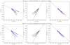 |
Fig. 7. Same as in Fig. 6, but for event IDs 5 and 6. |
| In the text | |
|
Fig. 8. Distributions of 3D tie-points sampling the VL comet tail in the reference frame of the comet trajectory: Xorb − Yorb coincides with the comet orbital plane; Zorb is perpendicular to it. The points tends to distribute along a curve lying in the orbital plane (left panel), while in the Zorb direction, the points are dispersed at most within ±0.04 R⊙. |
| In the text | |
|
Fig. 9. Set of syndyne curves in different colors and styles for β = 0.25, 0.50, 0.75, 0.95 plotted against the sample data points tracking the VL comet tail in the orbital plane of the comet. The orbit of the comet is given by the dashed red line. |
| In the text | |
|
Fig. 10. Propagation of the sungrazer comet in the Metis VL FoV. In the left panel the location of the comet is shown in the dashed white box. A zoomed-in time sequence of the comet is shown in the six panels on the right. The starting time of the zoomed-in images is 2021-12-24 at 21:41 UT, followed by the five frames taken on 2021-12-25. |
| In the text | |
|
Fig. 11. Sequence of 79 UV images acquired on 24 December between 20:09:30 UT (top left) and 22:45:30 UT (bottom right). Each image shows a zoom-in over the detector region (located near the southeast corner) where the comet was observed; each zoomed-in region is 30 × 30 bins, corresponding to 40.8 × 40.8 arcmin. |
| In the text | |
|
Fig. 12. Sequence of eight UV images obtained on December 24 between 20:09:30 UT (top left) and 22:45:30 UT (bottom right) after co-alignment and averaging over ten subsequent images. Each image shows a zoom-in over the detector region (located near the southeast corner) where the comet was observed; each zoomed-in region is 30 × 30 bins, corresponding to 40.8 × 40.8 arcmin. |
| In the text | |
|
Fig. 13. Average Lyman-α image resulting after the co-alignment and averaging of all 79 images acquired on 24 December 2021 between 20:09:30 UT and 22:45:30 UT. The position of the comet is indicated by the yellow box. |
| In the text | |
|
Fig. 14. Magnified image of the comet Lyman-α emission corresponding to the area surrounded by the yellow box in Fig. 13 and resulting after averaging between 20:09:30 UT and 22:45:30 UT on 24 December 2021. The coronal average background emission has been subtracted. |
| In the text | |
|
Fig. 15. Lyman-α intensity distribution across the cometary tail, going from the profile at the emission peak (light blue) to the profile at the end of the tail (dark blue). For each row the solid lines show the observed Lyman-α intensity, while the dotted lines show the corresponding Gaussian fits. Different colors in each curve correspond to different locations along the tail, going from the location of the comet nucleus (light blue) to the end of the tail (dark blue). |
| In the text | |
|
Fig. 16. Determination of solar wind speed and proton temperature from the analysis of the Lyman-α intensity distribution. Left: determination of the predominant tail orientation by linear fitting of the peak locations of Gaussian Lyman-α intensity distribution across the tail. Right: determination of the cometary Lyman-α tail semi-aperture angle. |
| In the text | |
|
Fig. 17. Location of the star Theta Ophiuchi in the Metis UV images at five different times between 23 and 25 December 2021 (the exact times are shown in the figure). The inner circle shows the location of the solar disk behind the Metis coronagraph occulter, while the diamond and triangle correspond respectively to the center of the solar disk and the location of the Metis Internal Occulter (IO). |
| In the text | |
|
Fig. 18. Lyman-α intensity distribution along the cometary tail, plotted as a function of distance from the location of the emission peak. Because of the comet’s relative speed with respect to the solar wind, the location of the comet nucleus is shifted by about 0.1 R⊙ with respect to the location of the Lyman-α emission peak. |
| In the text | |
Current usage metrics show cumulative count of Article Views (full-text article views including HTML views, PDF and ePub downloads, according to the available data) and Abstracts Views on Vision4Press platform.
Data correspond to usage on the plateform after 2015. The current usage metrics is available 48-96 hours after online publication and is updated daily on week days.
Initial download of the metrics may take a while.