| Issue |
A&A
Volume 679, November 2023
|
|
|---|---|---|
| Article Number | A52 | |
| Number of page(s) | 35 | |
| Section | Numerical methods and codes | |
| DOI | https://doi.org/10.1051/0004-6361/202347259 | |
| Published online | 03 November 2023 | |
Inverse-problem versus principal component analysis methods for angular differential imaging of circumstellar disks
The mustard algorithm
STAR Institute, Université de Liège,
Allée du Six Août 19c,
4000
Liège, Belgium
e-mail: This email address is being protected from spambots. You need JavaScript enabled to view it.
Received:
22
June
2023
Accepted:
25
September
2023
Abstract
Context. Circumstellar disk images have highlighted a wide variety of morphological features. Recovering disk images from high-contrast angular differential imaging (ADI) sequences is, however, generally affected by geometrical biases, leading to unreliable inferences of the morphology of extended disk features. Recently, two types of approaches have been proposed to recover more robust disk images from ADI sequences: iterative principal component analysis (I-PCA) and inverse problem (IP) approaches.
Aims. We introduce mustard, a new IP-based algorithm specifically designed to address the problem of the flux invariant to rotation in ADI sequences – a limitation inherent to the ADI observing strategy – and discuss the advantages of IP approaches with respect to PCA-based algorithms.
Methods. The mustard model relies on the addition of morphological priors on the disk and speckle field to a standard IP approach to tackle rotation-invariant signals in circumstellar disk images. We compared the performance of mustard, I-PCA, and standard PCA on a sample of high-contrast imaging data sets acquired in different observing conditions, after injecting a variety of synthetic disk models at different contrast levels.
Results. Mustard significantly improves the recovery of rotation-invariant signals in disk images, especially for data sets obtained in good observing conditions. However, the mustard model inadequately handles unstable ADI data sets and provides shallower detection limits than PCA-based approaches.
Conclusions. Mustard has the potential to deliver more robust disk images by introducing a prior to address the inherent ambiguity of ADI observations. However, the effectiveness of the prior is partly hindered by our limited knowledge of the morphological and temporal properties of the stellar speckle halo. In light of this limitation, we suggest that the algorithm could be improved by enforcing a data-driven prior based on a library of reference stars.
Key words: protoplanetary disks / techniques: image processing
F.R.S.-FNRS FRIA grantee.
F.R.S.-FNRS Postdoctoral Researcher.
F.R.S.-FNRS Senior Research Associate.
© The Authors 2023
 Open Access article, published by EDP Sciences, under the terms of the Creative Commons Attribution License (https://creativecommons.org/licenses/by/4.0), which permits unrestricted use, distribution, and reproduction in any medium, provided the original work is properly cited.
This article is published in open access under the Subscribe to Open model. This email address is being protected from spambots. You need JavaScript enabled to view it. to support open access publication.
1 Introduction
High-contrast imaging (HCI) is a particularly challenging field as its primary goal is to enable the detection of objects near very bright stars, such as exoplanets and circumstellar disks that are typically orders of magnitude fainter than their host star. The combination of advanced instrumentation with a relevant association of observing strategies and post-processing techniques is required to reveal the faint circumstellar signal hiding in the vicinity of the star. The majority of the starlight and aberrations caused by atmospheric turbulence are removed by the corona-graph and adaptive optics, respectively. However, in addition to the constraints of challenging observing conditions, a significant remaining limitation lies in quasi-static speckles that are not mitigated by the adaptive optics system (Cantalloube et al. 2019). Observing strategies such as angular differential imaging (ADI; Marois et al. 2006) provide a lever for post-processing techniques to differentiate between quasi-static speckles and the circumstellar signal. Angular differential imaging is an observing strategy in which the telescope pupil is stabilized with respect to the detector, and the field of view rotates over the course of the observation. The result is a sequence of images where the stellar halo and its associated speckles remain quasi-static over time, while circumstellar objects rotate with the field of view. Nowadays, ADI is the prime observing strategy used in most HCI surveys dedicated to searching for exoplanets and imaging circumstellar disks.
An important application of HCI techniques is the study of planet formation around young stars surrounded by protoplanetary disks, where planets are known to form. Recent observations with the Atacama Large Millimeter and submillimeter Array (ALMA) at submillimeter wavelengths and with the latest generation of HCI instruments at near-IR wavelengths have revealed a wide diversity of structures in these disks. It is as yet unclear how all these structures are connected to embedded planets since very few protoplanets have been unambiguously confirmed to date (e.g., Keppler et al. 2018; Haffert et al. 2019; Hammond et al. 2023). Principal component analysis (PCA) is currently one of the most used post-processing techniques for ADI sequences obtained for such systems. A common issue with PCA, and many state-of-the-art algorithms for ADI processing such as median-subtraction and locally optimised combination of images (namely Classical-ADI and LOCI; Marois et al. 2006; Lafrenière et al. 2007), is that it is designed to search for point-like sources and is not well suited for retrieving the geometry of extended disk signals. More specifically, ADI-based processing techniques have been shown to induce deformations on extended signals (Milli et al. 2012; Christiaens et al. 2019; Flasseur et al. 2021; Pairet et al. 2021). These deformations compromise the interpretability of disks imaged using ADI and hence also studies of their morphological features, such as asymmetries or spirals, which are potential indirect planet signatures and could inform on ongoing planet-disk interactions. Moreover, these deformations can also lead to false-positive protoplanet candidates due to the filtering of extended signals into compact (point-like) sources (e.g., LkCa 15 b,c,d; Currie et al. 2019). Algorithms that leverage reference star differential imaging do not suffer from self-subtraction and associated geometrical deformations (Ren et al. 2018; Ruane et al. 2019; Xie et al. 2022). However, satisfactory reference stars are not available for all data sets. Therefore, the main goal of the present work is to accurately deduce the true morphology of a disk solely from ADI sequences. Under these assumptions, our prime objective is to prevent any confusion between geometrical artifacts and real disk features, hence facilitating the interpretation of science images. In this context, some algorithms have been developed specifically for the imaging of extended sources in an attempt to prevent deformations. Two of them are based on inverse problem (IP) approaches (Flasseur et al. 2021; Pairet et al. 2021), and two others are based on an iterative-PCA (I-PCA) algorithm (Pairet et al. 2021; Stapper & Ginski 2022).
While these methods have been shown to provide a more robust recovery of disk images, they still suffer from the intrinsic limitation of ADI-based observations of not properly recovering rotation-invariant disk signals (also referred to as circular invariant flux in Juillard et al. 2022). Here, we present a new IP-based approach that aims to improve the recovery of rotation-invariant disk signals. In Sect. 2 we provide a general description of I-PCA algorithms and their limitations. Section 3 introduces our novel IP-based algorithm, mustard, and explains how it differs from previous IP-based implementations. Then, in Sect. 4, we present a series of tests on ADI data sets with injected synthetic disks to compare the performance of IP and I-PCA approaches. In light of this analysis, we discuss in Sect. 5 the advantages and drawbacks of IP approaches and provide recommendations as to which algorithm should be used to recover a disk from ADI sequences acquired in different conditions.
In the rest of the manuscript, we use the following notations: Y ∈ ℝn,m,m denotes the ADI sequence (also known as the ADI cube), with n the number of frames, and where each frame is a square image of size m × m pixels. Each frame, Yk, of the ADI data set is associated with a parallactic angle, θk. We use S ∈ ℝn,m,m to denote the cube of speckle fields reconstructed by a given algorithm, with Sk ∈ ℝm,m the speckle field in the kth frame and s ∈ ℝm,m the average speckle field. The 2D definite matrix d ∈ ℝ+m,m denotes the circumstellar signal. The estimate of a parameter is written with an over bar  . The PCA approximation of the ADI cube is denoted
  , where q is the number of principal components (PCs) that are kept in the singular value decomposition. This operator provides an estimation of the speckle field:
  . We use Rθ(x) to denote the rotation operator for one frame, x, by an angle θ, and Δθ is a scalar denoting the total parallactic angle variation in a given data set. We use Ƥ(x) to denote regularization fuctions Ƥ : ℝm,m → ℝ. All vector and matrix multiplications are based on the element-wise Hadamard product. The absolute value operator is written ||A||. The l1-norm
  is the sum of the absolute values of the elements in the vector or the matrix A, while the l2-norm
  is the sum of the absolute square values of the elements.
2 I-PCA for ADI sequences
Principal component analysis processing of an ADI sequence is based on the calculation of a PC basis through singular value decomposition of the ADI sequence, after the transformation of the image cube into a 2D (time vs. spatial) matrix. The PCA method creates a a model of the speckle field by projection of the ADI images onto a chosen number of PCs. Then the model is subtracted from the original images, so that the residual images contain less stellar light while preserving circumstellar signals (captured in high-order PCs) as much as possible (Soummer et al. 2012; Amara & Quanz 2012). Even with a wise choice for the number of components, this method is systematically aggressive toward extended signals, which are always partly subtracted and hence not well restored. This is largely due to circumstellar signals appearing partly in low-order PCs (Milli et al. 2012; Christiaens et al. 2019).
An iterative process, involving the reestimation of the speckle field and the removal of previous estimations, was introduced by Milli et al. (2012) using classical ADI (cADI). They concluded that this approach could assist in mitigating self-subtraction. Subsequently, leveraging PCA methods, I-PCA approaches were developed to iteratively refine the estimation of the speckle field in each frame by iteratively removing the estimated disk signal to prevent it from being captured in the principal components (and hence in the subtracted speckle field model):

where 𝒬: ℝm,m → ℝn,m,m creates an image cube of n frames, with each frame k containing the same disk image d rotated by the parallactic angle θk. The inverse operation 𝒬−1 : ℝn,m,m → ℝm,m corresponds to averaging the de-rotated cube of speckle field-subtracted frames. Throughout this paper, we use the GreeDS implementation of I-PCA described in Pairet et al. (2021). Our implementation of GreeDS was extracted from the MAYONNAISE package1 in order to be used independently. Our implementation is a re-factored version inspired from the original code, available on GitHub2 and providing some extra options (see the GitHub page for details).
Iterative PCA has been shown to provide better results in terms of disk image recovery than classical PCA (Pairet et al. 2021; Stapper & Ginski 2022), even though in their I-PCA tests on simulated data, Stapper & Ginski (2022) have observed disk deformations that depend on the disk morphology and on the available degree of rotation. A common limitation to any PCA-based method when working with extended signals is the poor handling of the circularly symmetric component of the signal (Flasseur et al. 2021). This limitation is inherent to the ADI strategy, as circularly symmetric components are invariant to field rotation. For a given disk, d, and amplitude of rotation, [θ0,θn], we defined flux invariant to the rotation fir ∈ ℝm,m as the matrix containing the minimum flux in each pixel for all considered parallactic angles, θk. This matrix can be expressed as follows:
![Mathematical equation: ${f_{ir}}:\forall \,x,y \in \left[ {0,m} \right],{f_{ir}}\left( {x,y} \right) = \mathop {\min }\limits_{0 \in \left[ {{\theta _0}..{\theta _n}} \right]} \,{R_\theta }\left( d \right)\left( {x,y} \right).$](/articles/aa/full_html/2023/11/aa47259-23/aa47259-23-eq7.png) (1)
(1)
State-of-the-art HCI algorithms suffer from a lack of a circularly invariant component in their output disk estimate due to their incapacity of distinguishing the part of the disk flux invariant to the rotation from a static component (i.e., speckle field).
A couple of examples of flux invariant to the rotation for different disk morphologies are shown in Fig. 1 for an amplitude of rotation Δθ = 60°. The deformations associated with rotation-invariant flux do not only appear in face-on disks, but are a systematic problem that appear in all disk morphologies. The rotation-invariant regions are more significant for wider disks, low inclination, and low amplitude of rotation. Leveraging the angular rotation only is not enough to correct for these deformations. Indeed, these regions are common to all frames, and thus share the same characteristic as the reconstructed speckles field. It is not always obvious to guess the initial disk morphology from the ADI post-processed images, considering the wide variety of geometries and substructures a disk can have. This limitation is inherent to the observing strategy, and can only be corrected by introducing additional information.
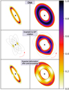 |
Fig. 1 Illustration of flux invariant to the rotation in disk images, showing two disk geometries (top), their region invariant to the rotation (middle), and the expected deformation induced by post-processing leveraging ADI (bottom). White areas are expected to be self-subtracted by post-processing. Intersections are computed with Python using ten frames evenly rotated between 0 and 60 degrees. |
3 Inverse problem approaches for ADI sequences
An IP approach is a statistical method that aims to estimate causal factors from the observed effects they produce. A general expression of the method can be defined by considering a set of observations (Y) corrupted by an error ϵ. The observations are the result of a known causal process (Forward model, ℱ) for a given set of input parameters (x). The residuals between observations and estimations of the data  are called the misfit. Ideally, if the model is a good description of the reality, the misfit should be equal to the noise ϵ. It is required to use an estimator to invert the process (Backward estimator), in order to find the optimal estimation
  that will minimize the misfit. The choice of the estimator is determined by the assumptions on the statistical distribution of the error ϵ. In the case of mean square error (MSE), ϵ is considered to be white noise, and the IP is described as follows:

![Mathematical equation: $\bar x = \mathop {\arg \min }\limits_x \left[ {{{\left| {Y - F} \right|}_{{l_2}}}} \right].\,\,\,\,\left( \rm{Backward estimator} \right)$](/articles/aa/full_html/2023/11/aa47259-23/aa47259-23-eq11.png)
According to the Hadamard conditions (Willoughby 1979), a well-posed problem requires that a solution (i) must exist, (ii) is unique, and (iii) changes continuously with the initial conditions. In most applications, the problem to be solved is, however, ill posed, which means that at least one of the Hadamard conditions is not fulfilled.
The key for an IP approach to tackle ill-posed problems is regularization (or constraint), which is the process of adding an extra source of information in order to circumvent the inherent ambiguities of the model, and transform the ill-posed problem into a well-posed problem. This practice, when used with temperance, can be a great tool for tackling difficult problems. The downside, however, is that artificially good results can easily be obtained based on unsubstantiated priors that do not correctly answer the addressed scientific questions. With the addition of regularization, an IP algorithm relies on the minimization of two terms: first, the data-attachment term given by the estimator and second, the regularization term(s) that aims to constrain the solution space with prior knowledge on x, leading to the following backward estimator:
![Mathematical equation: $\bar x = \mathop {\arg \min }\limits_x \left[ {{{\left| {Y - F\left( x \right)} \right|}_{{l_2}}} + \mu P\left( x \right)} \right].$](/articles/aa/full_html/2023/11/aa47259-23/aa47259-23-eq12.png)
When applying an IP approach, it is crucial to understand the scope of validity of the chosen forward model and its inherent ambiguities, to be aware of the validity of the prior added through regularization, and to wisely adjust its strength to guarantee robustness and trustworthiness of results. This is handled by the hyperparameter μ, whose goal is to define the regularization strength. The value of μ generally needs to be adjusted by the user to strike an appropriate balance between the data attachment term and the regularization. Overall, an IP algorithm is a flexible method that can be adapted in various manners by changing the estimator and regularization. One purpose of using an IP approach over an estimator like PCA is to provide a better interpretation of the data through a model, and by adding the lacking information through regularization.
Applied to ADI, the scientific task we wish to tackle with an IP algorithm is to reliably sort between speckle field and the azimuthally extended (circularly invariant) disk signal. However, ADI data sets are a very adversarial environment. We can sort the sources of errors into three categories: (i) inherent ambiguities of angular diversity (flux invariant to the rotation, small amplitude of rotation, uneven distribution of parallactic angles), (ii) data out of the scope of validity (fast varying speckles, wind-driven halo, undetermined noise statistics), and (iii) technical bottlenecks. The latter may include algorithmic elements, such as the limitations of the rotation operator in the discrete domain, or issues related to a specific method, such as non-convexity for gradient descent.
3.1 The mustard approach
Our motivation to propose a new IP algorithm for disk imaging in HCI is to focus on the inherent ambiguities of the ADI technique, as we noticed that no algorithm so far addresses this issue. We aim to correct for the geometrical biases of standard point-spread-function-subtraction techniques, which generally assign any rotation-invariant flux fully to the reconstructed speckle field, by making an assumption on its morphology.
In order to build a statistically viable IP backward model to estimate the speckle field, it is required to assume the speckle field as static despite its stochastic behavior. The forward model ℱ(s, d, k) that describes a frame Yk of the ADI cube is written as

The MSE estimator to invert this model is thus
![Mathematical equation: $\bar d,\,\bar s = \mathop {\arg \min }\limits_{s \in {R^{ + m,m}},d \in {R^{ + m,m}}} \left[ {\sum\limits_{pixels = 0}^{m \times m} {\sum\limits_{k = 0}^n {{{\left\| {{Y_k} - \left( {s + {R_{{\theta _k}}}\left( d \right)} \right)} \right\|}^2}} } } \right].$](/articles/aa/full_html/2023/11/aa47259-23/aa47259-23-eq14.png) (2)
(2)
By construction, modeling the speckle field as static is equivalent to estimating the average speckle field S ∈ ℝn,m,m as s ∈ ℝm,m. Ideally, variations in the speckle field will be attributed to the misfit, but this is not guaranteed.
Our IP is ill posed due to the overlap between d and s. Indeed, a component invariant to rotation can be labeled as either static (i.e., as s) or rotating (i.e., as d). To sort out these ambiguities, we had to use prior knowledge. For this purpose, we added a prior to the morphology of the speckle field through the definition of a regularization mask, Mreg, as a double-Gaussian profile representing the expected amount of rotation-invariant flux associated with the speckle field. This mask was used to define a regularization term Ƥmask, which will guide the flux invariant to rotation of  , defined as follows:

where the linear norm, l1, is weighted by the mask, Mreg.
In Fig. 2, we show the anticipated impact of using a mask made up of a double 2D Gaussian. The first Gaussian (dotted gray in the top-right panel) is meant to represent the inner halo primarily arising from stellar residuals near the center, while the second Gaussian (dashed orange) is intended to capture the spread of the diffraction pattern across the entire frame. For illustration purposes, the two 2D Gaussian models are derived by a fit to the mean de-rotated cube image (top middle panel) before introducing the disk signal, and then subtracted from the mean de-rotated cube after the disk signal has been injected (bottom-right panel). This example is meant to demonstrate the impact of subtracting an optimal mask, which would help resolve the circular ambiguities, even though it does not exactly illustrate the process undertaken by the algorithm when such a prior is added as a regularizer. Obtaining an optimal Gaussian mask using actual data is challenging since do not have access to an empty data set. In practice, when using mustard, the parameters of the double Gaussian are thus set manually, which limits the efficacy of this approach in real observations, highlighting the critical importance of mask selection. Nonetheless, by utilizing the mask as a form of regularization rather than relying on it solely for fitting (i.e., incorporating it into the forward model by decomposing the static speckles and the diffraction pattern), we mitigated potential inaccuracies that may arise from imperfect mask definition. In practice, the mask can be adjusted manually when using mustard in an attempt to minimize the distance between the model and the data. This regularization will be counterbalanced by the smoothness regularization and the data attachment term, both of which capitalize on angular diversity. Furthermore, the Gaussian approximation is suboptimal, as it fails to precisely describe the mean speckle field, including the bright circular halo around the region that is well corrected by the deformable mirror, at a radius of 0.″70 in the data shown here.
The parameters of the double-Gaussian mask have to be defined by the user when using mustard. Utilizing a more complex mask (e.g., learned from a library of coronagraphic observations of stars) could improve our results but goes beyond the scope of this study, which solely aims to leverage ADI, and will be investigated in a future work. Mustard is initialized with the mean de-rotated ADI sequence (as in a no-ADI data set) in order to assign all ambiguous flux to the disk as a first estimate. Hence, this regularization will push out the ambiguous flux that does not belong to the disk according to the shape of the mask. The mask regularization Ƥmask is defined as follows:
In addition, we defined a smoothness regularization term using the spatial gradient of the circumstellar and stellar signals d and s, respectively. It is a common regularization to compensate for noise (Benning & Burger 2018). With Δ standing for the Laplacian operator, the two regularization terms read

The three regularization terms are added to the dataattachment term, weighted by hyperparameters [μ1,μ2,μ3]. Additionally, a binary mask Mc is added to ignore pixels located under the coronagraphic mask, or too close to the optical axis. The final expression for the minimization reads as follows:
![Mathematical equation: $\matrix{ {\bar d,\bar s = \mathop {\arg \min }\limits_{s \in {{\rm{R}}^{{\rm{ + ,}}m{\rm{,}}m}},d \in {{\rm{R}}^{ + ,m,m}}} \left[ {\sum\limits_{pixels = 0}^{m \times m} {\left( {{M_c}\sum\limits_{k = 0}^n {{{\left\| {{Y_k} - \left( {s + {\alpha _{{\theta _k}}}\left( d \right)} \right)} \right\|}^2}} } \right)} } \right.} \hfill \cr {\left. {\,\,\,\,\,\,\,\,\,\,\,\,\,\,\, + {\mu _1}{\beta _{{\rm{mask}}}}\left( d \right) + {\mu _2}{\beta _{{\rm{smooth}}}}\left( d \right) + {\mu _3}{\beta _{{\rm{smooth}}}}\left( s \right)} \right].} \hfill \cr } $](/articles/aa/full_html/2023/11/aa47259-23/aa47259-23-eq18.png) (3)
(3)
A good balance between the morphological regularization terms and the data-attachment term is required to provide good results. Hyperparameters can be set based on the initialization, [d0,s0] of the disk and average speckle field, as a given percentage, pi, of the data-attachment term:
 (4)
(4)
where Ƥi,0 is the value of the regularization term i at initialization, namely Ƥsmooth(d0), Ƥsmooth(s0), and Ƥmask(d0), respectively. For the initialization of the disk d0, we used the positive mean de-rotated cube, while s0 was set as the mean positive residuals after subtracting the disk initialization from the cube:  .
.
Mustard is a Python object-oriented software package using PyTorch and its implementation of the Broyden–Fletcher–Goldfarb–Shanno algorithm (Avriel 2003), an iterative method for solving unconstrained nonlinear optimization problems. The Fourier-transform based image rotation used in mustard is a Torch tensor adaptation of its implementation in the VIP package3. The mustard package is available on GitHub4.
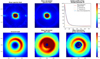 |
Fig. 2 Illustration of the capabilities of an optimal double-Gaussian mask to capture the rotation-invariant stellar residuals. The leftmost two figures in the first row respectively display the mean and the mean de-rotated speckle field before injection of the disk signal. The top-right figure displays the radial profile of the de-rotated empty data set (solid red line) together with the double-Gaussian fit, with the two Gaussians represented in dotted gray and dashed orange, respectively. The solid blue line represents the sum of the two Gaussians. The fit was performed while excluding the pixels within the numerical mask, which is an aperture with an 8-pixel radius. The bottom row shows, from left to right, the disk GT and the mean de-rotated cube after injection before and after subtraction of the optimal Gaussian mask. The figure scales are consistent across all images of each row. Axis values are in arcseconds. The intensity values displayed by the colorbar are arbitrary. This test was conducted using cube #2 with disk D injected at a contrast of 5 × 10⁻⁴. |
3.2 Previous IP approaches: MAYO and REXPACO
REXPACO (for Reconstruction of Extended features by PAtch COvariances; Flasseur et al. 2021) is an IP approach that includes a statistical model of noise inherited from the PACO algorithm (Flasseur et al. 2018). REXPACO and mustard are similar regarding the data-attachment term, but there are two main differences between these algorithms. Firstly, one of the regularization terms of REXPACO penalizes the l1-norm of the disk estimate, while in mustard we used a mask that aims to prevent flux ambiguous to the rotation from being systematically assigned to the speckle field estimate. Secondly, REXPACO enforces the statistics of the misfit by using the covariance patches approach from the PACO algorithm.
MAYONNAISE (or MAYO for short, Pairet et al. 2021, for Morphological Analysis Yielding separated Objects iN Near infrAred usIng Sources Estimation), is an optimization algorithm that introduces a morphological analysis of the disk and planets after the speckle field estimation of the I-PCA algorithm, GreeDS. It differs in the way it addresses the problem: contrary to REXPACO and mustard, MAYO estimates a different speckle field for each frame. To not have the speckle field described as an unknown stochastic phenomenon, MAYO forces the speckle field S to be described as a linear combination of the q first PCs estimated through I-PCA. One of the main goals of MAYO is to deconvolve the circumstellar signal, and to separate pointlike sources from extended disk signals. The model therefore contains the convolution by the point spread function, and the disk and planet models are constrained by morphological priors using shearlets and point-like sources, respectively. Additionally, it uses a Huber loss estimator (instead of MSE) because this distance is strongly convex at the neighborhood of 0 and affine at its boundary, and hence less sensitive to outliers in the data than the squared error loss.
To understand the specifics of each algorithm, and what kind of answer they can provide, it is necessary to comprehend the underlying assumptions made by the equations used in each model, and their dependences. Estimators that are grounded in physics and rely on well-established probabilistic methods are generally more convincing. They are considered more interpretable and reliable, although this may vary depending on the specific context and application (Sengijpta 1995). The assumptions made by each algorithm are summarized in Table 1, and further discussed in the following bullet points, along with their estimator properties.
The PCA model treats the speckle field as the PCs of the singular value decomposition (SVD). This is an efficient method for removing the quasi-static part of the stellar halo, but it is too aggressive and can remove a significant part of the circumstellar signal (self-substraction, Milli et al. 2012; Christiaens et al. 2019; Stapper & Ginski 2022). Additionally, it does not introduce any physical assumptions, such as the positivity of the disk signal, which could potentially lead to more accurate results.
The I-PCA algorithm provides a PCA-based estimation of the disk while also enforcing the positivity of the disk signal. This approach corrects PCA self-subtraction effectively, but it does not correct for flux invariant to rotation.
MAYO implements a morphological analysis by modeling the circumstellar signal as the sum of shearlet-based components and point-like sources. This model provides a prior for the deconvolution task, leading to visually appealing outputs resembling disks (i.e., enforcing smoothness, sharpness, or sparsity without statistical justification). However, the assumption of a unique speckle field for each frame is too unconstrained, which hinders the algorithm’s ability to improve upon the initial estimate provided by the I-PCA. Moreover, a morphological analysis alone may not be sufficient to differentiate between signals and artifacts, as there is no distinct morphological component that characterizes them unambiguously. Therefore, it becomes necessary to limit the number of shearlets and planets, which could lead to an erasure of the compact signals, fine structures in the disks, or planets. Overall, the MAYO estimator suffers from identifiability issues: multiple sets of parameter values can fit the data equally well when the model is unconstrained, potentially resulting in ambiguous or unreliable estimation results (Maclaren & Nicholson 2019). The algorithm is prone to inheriting imperfections from the initial speckle field estimation process, so that its performance depends on the choice of rank and iteration parameters used in the I-PCA.
The REXPACO algorithm uses an IP approach that introduces an estimation of the noise statistics and enforces the positivity of the signal. Along with mustard, the two algorithms do not use a PCA estimation to model the speckle field. However, to do so, these algorithms must assume that the speckle field is static. These estimators suffer from adequacy issues: the optimality of the probabilistic-based estimator is no longer guaranteed due to the model’s failure to adequately represent the underlying system (Schiff 2011). If the static assumption made on the speckle field is not fulfilled, then the underlying assumption that the misfit is white noise is invalid, and some speckle field variations will be fit “at best” into the rotating components (disk and planets) estimates. This can be the case for data sets acquired in challenging observing conditions or, more generally, for disks that are significantly fainter than the amplitude of speckle variations. In such cases, PCA-based estimations will better handle the variation in flux and speckle morphology between frames, by projecting each frame onto a well-chosen number of PCs.
So far, mustard is the only approach that attempts to address the limitation of flux invariant to rotation, but it does not provide strong guarantees of robust disk image extraction as the parameters (width and amplitude) of the Gaussian mask have to be assumed a priori.
Finally, one of the main limitations to the recovery of extended sources from ADI sequences is the wind-driven halo. This type of nuisance elongates the stellar halo in a specific direction, creating a butterfly pattern (Cantalloube et al. 2019). Its structure varies throughout the acquisition, and rotates in a similar way as the field during ADI sequences. Despite being very common, this phenomenon goes beyond the scope of validity of all IP algorithms to date.
Comparison of assumptions made in the PCA, I-PCA, REXPACO, MAYO, and mustard algorithms with respect to reality.
4 Performance comparison
In this section, we conduct a comprehensive study to test the performance of mustard on a range of synthetic disks, and compare it with results obtained with PCA and I-PCA methods. We leave a complete performance comparison with other IP-based algorithms to a future disk imaging data challenge, where the developers of each method will have a chance to fine-tune their algorithm and provide the fairest possible comparison (more about this can be found in Sect. 5.2). We still provide in Sect. 4.4 a couple of examples of mustard results on data sets that have been previously processed by MAYO and REXPACO in the literature.
4.1 Sample data sets
To explore the disk imaging performance of the selected algorithms, we considered four empty data sets that reflect different observing conditions (see the details in Table 2), in which we injected five disk models with diverse morphologies (see the first row of Fig. 3). Specifically, we selected empty data sets from the 150 targets of the SpHere INfrared survey for Exoplanet (SHINE-F150; Desidera et al. 2021; Langlois et al. 2021) taken with the Very Large Telescope (VLT) using the coronographic instrument SPHERE (Spectro-Polarimetric High-contrast Exo-planet REsearch). These data sets were obtained through the SPHERE Data Center, with the following characteristics: low Strehl ratio with 26° rotation (ID#1), wind-driven halo (ID#2), unstable speckle field (ID#3), and good Strehl ratio with 80° rotation (ID#4). The disk morphologies were carefully chosen to represent a range of possible cases for debris and protoplanetary disks. These include two 75° inclined disks with different levels of sharpness (disks A and B), a 45° inclined disk with two concentric rings (C), one face-on disk with some azimuthal flux variation (D), and a hydrodynamical simulation computed with Phantom (Price et al. 2018) and processed with MCFOST (Pinte et al. 2006), representing a central protostar and a low-mass companion embedded in a protoplanetary disk (E). The simulation aims to reproduce the morphology of the protoplanetary disk around MWC 758, and its exact setup is detailed in Calcino et al. (2020). The two concentric rings in disk C were chosen to be nearly resolved. The gap between the two rings has a width of 5.3 pixels, whereas the full width at half maximum (FWHM) of our various test cubes ranges from approximately 4–5 pixels.
The five synthetic disks were injected at three contrast levels (10−3, 10−4, and 10−5), to generate a total of 60 data sets. The contrast at which the disks are injected is defined as the integrated flux measured in an FWHM-sized aperture centered at the peak intensity of the disk, divided by the integrated flux in a FWHM-sized aperture of the point spread function. An exception was made for the synthetic disk E, where the flux is measured at the companion location.
4.2 Metric
To assess the quality of the disk estimations obtained with the different algorithms, we considered various metrics that are relevant to measure morphological deformations with respect to the GT image:
the structural similarity index measure (SSIM), which captures the disparity of contrast, luminance, and structure on various windows of the two images (Wang et al. 2004);
the Spearman’s rank correlation coefficient, which assesses how well the relationship between the GT and the reconstructed images can be described using a monotonic function;
the Euclidean distance, which is the square root of the sum of the squares of the pixel intensity differences between the two images;
the Pearson correlation coefficient, which assesses the degree of linear correlation between the two images;
the sum of absolute differences (SAD), which is calculated by summing the absolute differences between each pixel of the two images.
We selected SSIM as our preferred metric, as it is a combination of metrics covering multiple aspects of image similarity, with demonstrated performance in achieving similar assessment of structural differences as human visual perception (Wang et al. 2004). However, we wish to emphasize that no single metric is better than all others in all aspects. Each metric provides different information: for example, the Spearman rank correlation coefficient better captures the global morphological difference, while the Euclidean distance is more sensitive to stellar residuals near the coronagraphic mask and/or ring-like noise artifacts in the image. Moreover, ranking disk image estimation is a multifactorial problem that often necessitates finding a satisfactory compromise between less geometrical biases and fewer noise residuals. Nevertheless, we observe that the cases where all metrics agree on the best algorithm correspond visually to disk images that are unambiguously better than others. Furthermore, despite disparities between metrics, we observe that they share common trends in their rankings.
The field of view considered for calculating the metrics also affects the results. We first calculated the metrics using a 1″-radius aperture, excluding a 6-pixel radius inner circle located behind the coronagraphic mask. A second set of metrics was then computed considering only pixels that are part the disk image in order to test disk reconstruction only, that is to say, ignoring the effect of both stellar residuals near the coronagraphic mask and background artifacts on the metrics. We summarize the results of our systematic tests in Fig. 4. Additional figures showing which algorithm achieves the best estimation for each disk, as inferred by each metric and for these two different cases, are presented in Appendix A (Figs. A.2 and A.3).
Data sets used in our study obtained in the H2 band with the IRDIS camera of VLT/SPHERE within the SHINE-F150 survey (Desidera et al. 2021; Langlois et al. 2021).
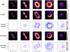 |
Fig. 3 Disk estimations for a contrast of 10−3 injected in the ADI cube no. 4 (see Table 2). Top: GT (injected disk images). Second and third rows: I-PCA estimation using GreeDS implementation and its residuals. Last two rows: mustard estimation and its residuals. In the residual maps, we emphasize the missing disk signal in blue, and excess signal in red. To highlight morphological biases only (i.e., not absolute flux recovery), disk estimations were rescaled in flux before the computation of the difference with the ground truth (GT) to obtain the residuals. The rescaling factors correspond to the flux ratio in a FHWM aperture located at the brightest pixel in the disk GT. Axis ticks are in arcseconds. |
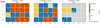 |
Fig. 4 Results of our systematic tests to compare PCA, I-PCA (GreeDS), and mustard. Each cell represents a different synthetic data set, and its color indicates which algorithm performed best according to the SSIM metric. The five disk morphologies are labeled along the x-axis (see Fig. 3 for details), the four empty data sets used for injection along the y-axis (see Table 2 for details), and the three contrast levels in the left (10−3), middle (10−4), and right (10−5) plots. White letters on a cell indicate which algorithm(s) did not detect the disk (p stands for PCA, g for I-PCA, and m for MUSTARD). Gray cells mean that no algorithm detected the disk. Black stars indicate that all five metrics (SSIM, Spearman, Pearson, Euclidean, and SAD) selected the same winner. |
4.3 Results
We tested the performance of classical PCA, I-PCA (GreeDS), and mustard in recovering the injected disks across our 60 data sets. We optimized the parameters of I-PCA and PCA by computing a series of disk estimates with different ranks (ranging from 1 to 5), for a maximum of 10 iterations per rank in I-PCA, and selecting the estimate that performed best according to the SSIM metric. When increasing the rank in the I-PCA algorithm, we retain the last iteration of the previous rank, which means that the case {rank=x, iteration=y} corresponds to (x − 1) * 10 + y iterations in total. For I-PCA, we excluded the first iteration from the selection, as it is equivalent to classical PCA. For mustard, while fine-tuning of the regularization mask from a data set to another is expected to improve our results, we instead considered a realistic scenario of not having access to the GT speckle field profile (due to the potential presence of a disk). Hence, unlike what was shown in Fig. 2, we did not make use of the empty data set, which is generally not accessible to the user, and rather attempted to tune the parameters of the double-Gaussian mask to minimize the distance between the data and our mustard model. We manually chose the regularization weights based on one data set (cube no. 4, disk D, contrast 10−3), and applied these weights to all data sets. Specifically, we set the regularization percentage at initialization (see Eq. (4)) to be pmask = 5%, psmooth,d = 5%, and pSmooth,s = 5%.
In Fig. 3, we present the results of I-PCA and mustard for a contrast of 10−3 using data cube no. 4 (a stable data set with favorable observing conditions) to highlight the main geometrical biases. To isolate these biases, we ignored flux inconsistencies by recalibrating the extracted disk images based on the integrated flux in a 1-FWHM aperture located at the maximum intensity of the GT disk, before computing the residuals. We used a color scale where blue indicates missing signal and red indicates excess. We observe that missing signal in I-PCA estimates is symptomatic of flux invariant to rotation. Disks A and B only show missing flux close to the coronagraphic mask, while disks C, D, and E show more flux invariant to rotation, leading to more significant deformations. The mustard IP approach can significantly reduce geometric biases related to flux invariant to rotation. However, it shows more noise residuals, especially in the region close to the coronagraphic mask and at the edge of the well-corrected region by the SPHERE deformable mirror (also known as the control ring), which may be due to the mask Mreg and/or the balance of regularization not being appropriate to the morphology of the speckle field. The sub-optimality of Mreg could have been corrected by estimating the mask from the empty data cube, but this would be unfair to the other algorithms. In the future, adapting the mustard ADI algorithm using a reference star as a data-driven prior is a potential avenue of improvement, as discussed in Sect. 6.
The disk reconstructions, along with the names of the best algorithms, as inferred by each metric, are presented in Appendix B. Regardless of the chosen metrics (see Appendix A), we observe that mustard can provide good results in the most favorable cases, namely bright disks in data sets with a close to static speckle pattern. Mustard performs particularly well for disks that contain more flux that is invariant to rotation (i.e., disks C, D, and E, the more face-on disks from our samples). In contrast, I-PCA is more robust in more challenging cases, performs better than simple PCA in most cases, and outperforms mustard in most cases where either the speckle field is unstable or the contrast is deeper than 10−4. We also note that the sharp-edged disk (A) is systematically better estimated by I-PCA than mustard. This is likely due to the minimal amount of rotation-invariant flux in this disk, which means that its overall morphology is not much distorted with I-PCA, with the resulting image containing less background noise and stellar residuals near the coronagraphic mask than the one obtained with mustard.
4.4 Tests on real data
Here, we present a comparative analysis of disk imaging for two ADI data sets already processed with MAYO and/or REXPACO in the literature. The first data set was obtained on PDS 70 (ESO program ID 1100.C-0481) in the K1 band with the infrared dual-band imager and spectrograph (IRDIS) camera of the Spectro-Polarimetric High-contrast Exoplanet REsearch corono-graphic system of the Very Large Telescope (VLT/SPHERE) in March 2019, under excellent conditions (seeing: 0.″39, wind speed: 4.45 m s−1, Δθ = 56°5). This data set had previously been processed using PCA (5 PCs) in Mesa et al. (2019). The same data set was processed with the MAYO and REXPACO algorithms, respectively in Pairet et al. (2021) and Flasseur et al. (2021). The second ADI data set was obtained with the same instrument and camera on RY Lupi (HIP 78094) in March 2016 (ESO program ID 097.C-0865) in the H2 band under excellent conditions (seeing: 0.″25, Strehl ratio 78%, Δθ = 71°). The data set was reduced using cADI and no-ADI (averaging after de-rotation without subtraction) in Langlois et al. (2018), and with REXPACO in Flasseur et al. (2021). The reader is referred to the original papers for the MAYO and REXPACO results, which we do not reproduce here for the sake of conciseness. In all cases, we observe that the MAYO and REXPACO algorithms, as well as mustard and I-PCA (see below), perform better than the original cADI or PCA reductions at restoring extended signals.
We processed the PDS 70 data set using mustard and I-PCA, and we compare in Fig. 5 the disk estimation and the averaged estimated speckle field obtained with these two algorithms. In the speckle field estimation of I-PCA, we observe a suspicious arc at a radius of ~0.″4, which matches the location of shadows in the disk estimate (red arc and green arrows in Fig. 5, respectively). This indicates that flux invariant to rotation is likely missing from the disk estimate, which could bias the interpretation of the final image, and potentially enhance an arm-like structure observed to the northwest. We observe the same signpost of missing flux invariant to rotation in the MAYO images (Fig. 9 in Pairet et al. 2021) and in the REXPACO images (Figs. 11 and 12 in Flasseur et al. 2021). Although MAYO performed deconvolution of the signal and separated point-like sources from the disk signal, we observe that the shearlet transform appears to have fitted the deformation inherited from I-PCA instead of correcting it. The MAYO image indeed suggests two point-like features (PLFs), among which PLF 2, at the east of the coronagraphic mask (Fig. 9 in Pairet et al. 2021), likely corresponds to a filtered spiral-like signal (or to bright stellar residuals near the coronagraphic mask). Based on our mustard images, we propose an alternative interpretation of the disk: the overall shape is closer to a regular ellipse, without shadows, and the arm-like structure to the northwest is real, but less prominent. This is inferred solely from the shape of the average speckle field. In Juillard et al. (2022), we confirmed that the observed structure exists at the northwest and deviates from what we would expect for a double-ring disk.
The disk and average speckle field estimates obtained using I-PCA and mustard for RY Lupi are presented in Fig. 6. The primary ring of the disk is correctly imaged by all algorithms, but the spiral-like features (Langlois et al. 2018) are better restored with I-PCA, mustard and REXPACO (Figs. 11 and 12 in Flasseur et al. 2021). The cADI (Fig. 1 in Langlois et al. 2018) is too aggressive toward these fine structures, while the no-ADI reduction hides them in the stellar halo. Compared to I-PCA, the interpretation of the disk by mustard does not provide much additional information because, unlike PDS 70, RY Lupi does not contain much bright signal that is ambiguous with respect to the 71° field rotation.
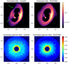 |
Fig. 5 Images of a VLT/SPHERE/IRDIS K1 data set on PDS 70 obtained using I-PCA (left) and mustard (right). The top row displays the estimated circumstellar signal, while the bottom row shows the mean estimated speckle field. The color scale is arbitrary (yet consistent between all plots in relative terms) and displayed in a logarithmic scale. The green arrows indicate the location of shadows in the disk, which are the consequences of the lack of circular component in the disk, and are consistent with the location of a bright arc (highlighted in red) in the speckle field estimation. |
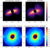 |
Fig. 6 Same as Fig. 5 but for a VLT/SPHERE/IRDIS H2 data set obtained on RY Lupi (program ID 097.C-0865, 2016). |
5 Discussion
We conducted a comprehensive evaluation of state-of-the-art algorithms for processing ADI data sets containing disks, aiming to determine their respective scope of validity. Our analysis involved systematic testing of PCA, I-PCA (GreeDS), and mustard on a diverse set of 60 synthetic data sets, encompassing various observing conditions and disk morphologies. Additionally, we compared the performance of these algorithms on a selection of real data sets. This comparative study enables us to analyze the strengths and limitations of the mustard IP approach with respect to PCA-based methods, focusing on three key aspects: (i) theoretical faithfulness, (ii) results, and (iii) automation/practicality (see Sect. 5.1). Subsequently, in Sect. 5.2, we explore the distinctions between the state-of-the-art IP algorithms and assess their respective use cases, identifying scenarios where one algorithm may outperform the others.
5.1 Static speckle model versus PCA-based estimation
In terms of faithfulness, no algorithm can provide a deformationfree disk due to the flux invariant to rotation and the absence of a perfect model to describe the quasi-static behavior of the speckle field. As seen in Fig. 3, the limitation associated with flux invariant to rotation can significantly impact disk morphologies, even in inclined disks. Mustard is the only algorithm that will not systematically exclude rotation-invariant flux from the disk estimate, but the fate of this component will still depend on the chosen prior (Mreg). Apart from this issue, the IP approach employed by mustard and REXPACO offers improved theoretical faithfulness compared to PCA-based methods. This is achieved by leveraging a concrete and constrained model of the ADI cube. However, this approach relies on the assumption that the speckle field remains static, meaning that there are minimal relative variations in the speckle field with respect to disk signal. In other cases, PCA-based methods can in practice be a good approximation to model the speckle field, and hence a relatively robust disk image, despite not providing any theoretical faithfulness.
In terms of results, we observe that I-PCA performs significantly better than PCA for restoring extended signals regardless of cube quality, contrast, and disk morphology (as also noted in Stapper & Ginski 2022). With an increasing number of iterations, more disk signal is recovered, but more noise residuals are also propagated and amplified, leading to strong background artifacts when using a large number of iterations. One example is the estimation of Disk A in Cube 2 with a contrast of 10−5 (as shown in Fig. B.15), which was processed using a rank of three and one iteration, totaling 2 × 10 + 1 = 21 iterations (see Sect. 4.3). We note that our iterative optimization method and I-PCA implementation may not be optimal in all cases: for example, high-contrast disk estimates may be improved by starting to iterate at a higher rank. A better optimization of I-PCA, including additional strategies such as thresholding, masking, or using temporal-PCA, could still improve the results (Stapper & Ginski 2022; Long et al. 2023). In general, we observe that mustard is the best algorithm in the most favorable cases (bright disk, stable data sets), achieving both minimal reconstruction errors and optimal flux estimation, especially for disks that contain more flux invariant to rotation as mustard partially assigns the ambiguous flux to the disk estimate, according to a prior. However, mustard does not perform well at high contrasts, and is more prone to contain circularly invariant artifacts, especially near the coronagraphic mask region, which explains why it is less often selected as the best reconstruction algorithm by metrics calculated on the whole field of view than calculated on the pixels of the disk only (see Appendix A). These artifacts are caused by the inappropriate assumption about the static behavior of the speckle field, and the imperfect regularization mask. Indeed, in addition to the difficulty in estimating the parameters for shaping the mask, we can observe in Fig. 2 that the double Gaussian assumption appears inappropriate for capturing the innermost region, as well as the bright speckle ring at a separation of ~0.″7 (i.e., the edge of the region corrected by the deformable mirror). Consequently, for high relative variations in the speckle field with respect to disk signal, the disk gets drowned in the stellar residuals.
In terms of practicality, automating the process of setting hyperparameters is a known limitation of IP approaches in general. In the case of I-PCA, finding the correct number of iterations and rank is crucial as the algorithm does not guarantee convergence for an increasing number of iterations, making it unclear when to stop and which image to consider as the final result in a real-world scenario. Despite this, compared to IP approaches, I-PCA is more intuitive, faster, and easier to parametrize, and the evolution of frames generated through the iteration can be used to facilitate the process. Additionally, another factor to account for in terms of algorithm practicality is computation time, which heavily relies on the implementation approach. The mustard, MAYO, and GreeDS algorithms (assuming ten iterations per rank for ten ranks) are implemented using the PyTorch package in Python. For a data set comprising 100 frames with dimensions of 256 × 256, the computational duration for the three algorithm implementations is roughly 20 min, 1 day, and a few seconds, respectively (2.8 GHz Intel Core i7 CPU; 16Go RAM). Alternative implementations of I-PCA utilizing NumPy might require a few minutes to process.
5.2 Comparison of IP approaches
It is challenging to make a fair comparison of empirical results between different IP approach algorithms, such as REXPACO, MAYO, and mustard, due to inconsistencies in the test methodology used in the respective publications. The quality of the data cubes in which the synthetic disks are injected, including the Strehl ratio, variability of the speckle field, amplitude of rotation, or presence of wind-driven halo, can significantly influence the results. Additionally, the definition of contrast for disks may not be equivalent in all publications. In this paper, we find that disks with contrasts ~10−5 were hardly detectable, whereas in Flasseur et al. (2021), cADI was able to recover disks with similar contrasts reasonably well, even though cADI is not known to perform better than PCA (Cantalloube et al. 2020). Similarly, Pairet et al. (2021) claim that it is possible to detect disks with contrasts as deep as 10−9, which is outside the range of contrast typically tested for algorithms thus far, for both disks and planets. Moreover, evaluating contrast at a single peak point, as performed in this paper, might not accurately depict the contrast of extended sources, especially for disks that exhibit a high peak that gradually diminishes in intensity as one moves away from the peak. More detections would have been possible if the intensity was uniform across all pixels of the disk. As a result, the ambiguity of this contrast definition persists. Therefore, only a standardized test pipeline such as the Exoplanet Imaging Data Challenge (Cantalloube et al. 2020, 2022) would provide a fair empirical test to compare different IP approaches. One can still highlight specific features in the results obtained by these various algorithms, and make some recommendations regarding their usage.
A specific feature of MAYO is that it includes an interesting interpretation of the deconvolved disk and planet. However, its model lacks identifiability (see Sect. 3.2). When using MAYO to retrieve disks from ADI sequences, one should systematically check the I-PCA first estimate provided by GreeDS to locate potential artifacts and ambiguities that could be overfitted. Due to the lack of statistical validity, we observe that the algorithm tends to fit deformations rather than correcting them (see Sect. 4.4). Consequently, in terms of faithfulness, MAYO does not provide a significant improvement over GreeDS.
Unlike other algorithms, mustard specifically tackles the issue of flux invariant to rotation. It provides a less aggressive interpretation of the disk that keeps more flux invariant to the rotation according to a prior, using a mask that has to be adapted by the user. However, it is limited by our imprecise knowledge of the speckle field, and the arbitrary choice of the mask Mreg and regularization weights μ may significantly alter the results. Nevertheless, mustard is particularly useful for disks that have a significant amount of flux invariant during rotation, and are brighter than the variations in the speckle field.
In terms of automation, each IP approach proposes an automated or semiautomated method for setting the hyperparameters. REXPACO and MAYO propose automated methods that search for optimal hyperparameters by minimizing the data-attachment term using regression algorithms. However, these techniques can be time-consuming and assume that the data-attachment term provides an ideal description of the data, which is not always the case (see Sect. 3.2). Consequently, achieving the global minimum of the data-attachment term might not necessarily result in the optimal disk estimate. On the other hand, mustard suggests defining regularization as a percentage of the data-attachment term. While this approach lacks statistical guarantees on the results, it can provide users with more intuitive parameter setting capabilities.
6 Conclusion
We have introduced mustard, an IP approach designed to address the recovery of flux invariant to rotation in circum-stellar disk images, which is an inherent limitation of the ADI observing strategy. No algorithm had specifically addressed this limitation before mustard, which hence provides an alternative interpretation of disk imaging data sets, with a better preservation of the flux invariant to rotation. We have also provided a comprehensive comparison of state-of-the-art algorithms to retrieve extended disk signals from ADI sequences and discuss their advantages and limitations. Mustard is suitable for stable data sets that fall within its scope of validity. However, it exhibits limited robustness when confronted with large relative variations in the speckle field compared to the disk signal. Iterative PCA proves to be more resilient in handling high-contrast scenarios, unstable speckle fields, and mild wind-driven halos. Our analysis suggests that, in most cases, I-PCA outperforms mustard and should be the preferred choice for recovering disks from ADI sequences. This recommendation is based on I-PCA’s combined performance and practicality, even though it does not completely address the challenges of flux invariant to rotation, nor provide statistical guarantees. Considering these factors, I-PCA serves as a solid initial approach to take before considering more sophisticated methods. Nevertheless, mustard, REXPACO, and MAYO can be utilized when their scope of validity and purpose align with the specific application scenario. For instance, mustard is particularly useful for recovering rotation invariant flux, while REXPACO offers enhanced guarantees and MAYO excels in decon-volution tasks. The choice of method depends on the specific requirements and goals of the application at hand.
An enhancement to a model-based approach such as mustard could be achieved by incorporating a mathematical model that describes the temporal evolution and morphology of the speckle field and accounts for known nuisance phenomena, such as the wind-driven halo. These limitations currently impact the quality of the model, resulting in challenges when recovering disks at higher contrasts. Therefore, there is a need to develop a more realistic and constrained model that effectively correlates with the observed data, addressing these limitations and improving the overall performance of mustard. Ambiguities related to flux invariance during rotation are a limitation specific to ADI observing strategies. Approaches that incorporate reference stars (star hopping/RDI) do not face this particular ambiguity. Some of the most notable efficiency gains compared to the PCA/median subtraction technique were obtained by leveraging RDI and imposing non-negativity constraints on the components employed to represent the estimated speckle field, through nonnegative matrix factorization of the reference images, and either a concurrent search for an optimal scaling factor of the model speckle field or data imputation (Ren et al. 2018, 2020).
Moreover, combining diverse observing strategies might assist in mitigating the distinct weaknesses of each approach, as exemplified by Lawson et al. (2022), who merged RDI with PDI, or by Flasseur et al. (2022), who merged ADI with SDI. Therefore, to address the inherent ambiguities of ADI, we propose exploring the combination of ADI with RDI in a future work. Reference stars provide reliable data-driven priors that can be used to solve the problem of the flux invariant to rotation. The combination of ADI with reference stars could, theoretically, offer the advantages of both methods: improving the correlation between the estimated speckle field through ADI and solving ambiguities that limit angular diversity through the use of reference stars. This can improve both I-PCA methods, by concatenating reference frames in the cube to compute the PCs, and IP approaches, by building the optimal prior through regularization based on the reference data. This will be the subject of future work (Juillard et al., in prep.).
Acknowledgements
This project has received funding from the European Research Council (ERC) under the European Union’s Horizon 2020 research and innovation program (grant agreement no. 819155), and from the Belgian Fonds de la Recherche Scientifique - FNRS. This work has made use of the SPHERE Data Centre, jointly operated by OSUG/IPAG (Grenoble), PYTHEAS/LAM/CESAM (Marseille), CA/Lagrange (Nice), Observatoire de Paris/LESIA(Paris), and Observatoire de Lyon (Galicher et al. 2018; Delorme et al. 2017). We are very grateful to Benoit Pairet and Laurent Jacques for their feedback on this work and useful discussions, and to Julien Milli, Philippe Delorme, and Mariam Sabalbal for their help in selecting, providing, and pre-processing the empty SPHERE data cubes used for the tests.
Appendix A Comparison of results for different metrics
This Appendix presents the results of the performance comparison for the three considered algorithms (PCA, I-PCA (GreeDS), and mustard) in terms of the inferred disk image, for each test data set described in Sect. 4.1, using the five different metrics described in Sect. 4.2: the SSIM (Wang et al. 2004), the Spearman’s rank correlation coefficient, the Pearson correlation coefficient, the Euclidean distance, and the SAD. Two sets of results are presented. The first set of results in Fig. A.2 shows the metrics computed considering a 1″-radius field of view, while the second set of results in Fig. A.3 shows metrics calculated on disk pixels only, defined considering the 85 percentile of the GT disk’s intensity (Fig. A.1).
 |
Fig. A.1 Mask used to compute metrics and considering only pixels of the disk. |
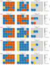 |
Fig. A.2 Same as Fig. 4 but for the five different metrics defined in Sect. 4.2 (from top to bottom): SSIM, Spearman’s rank, Pearson correlation, Euclidean distance, and SAD distance. |
For each subplot within these two figures, the cells represent different test data sets. The color of the cell indicates which algorithm performed the best according to the respective metrics. We simulated five different disk morphologies (x-axis, A→E), injected them in four different empty data sets of stars observed with the IRDIS camera of the VLT/SPHERE instrument under various conditions (y-axis, 1→4), and tested our three algorithms for injections at three different contrast levels: 10−3 (left), 10−4 (middle), and 10−5 (right). The five different disk morphologies are illustrated in Fig. 3, while details on the four empty data sets can be found in Table 2. Gray cells mean that no algorithm detected the disk. White letters on a cell indicate which algorithm(s) did not detect the disk (p→PCA, g→I-PCA, m→MUSTARD). Black stars indicate that all five metrics (Spearman, SSIM, Euclidean, Spearman, Pearson, and SAD) agree on the algorithm which achieved the best disk estimation.
From these two figures, it can be observed that the various metrics yield relatively similar results. Mustard is more frequently chosen as the best reconstruction by all metrics for low contrasts (10−3) and for the more face-on disk (C, D, E). However, when considering the entire image, I-PCA is preferred in most cases, with an average selection rate of 53% across all metrics (considering detection only). In comparison, mustard is selected on average 37% of the time, while PCA is selected only 10% of the time. We note that these rates exclude the non-detections, which represent 26% of our 60 simulations. When considering only the disk pixels and using the Spearman’s rank correlation coefficient, which are better suited for assessing the preservation of global morphology and are less sensitive to background noise and image residuals, the results generally favor mustard.
Appendix B Results of disk estimations
This Appendix presents the disk estimations obtained with PCA, I-PCA (GreeDS) and mustard for all 60 test data sets considered in this work (Figs. B.1–B.20). Each page-sized figure presents the results for a specific synthetic disk in a given data sets.
The color bar bounds in the residual plots is set to ± maximum of intensity of the GT, centered at 0. For the disk image estimation plots, the color bar is adjusted for each data set to have a maximum value equal to the 99th percentile of the image. The minimal value is set to 0. Additionally, the optimal PCA and I-PCA parameters (rank and number of iterations) are written at the top left of the corresponding images.
Page-sized figures for each data set are ordered from the easiest data cube (ID#4, stable) to the hardest (ID#1, low Strehl ratio), and from the most face-on disk (disk E) to the sharpest one (disk A), in order to illustrate the most significant improvements brought by the mustard model in the first pages of this annex.
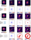 |
Fig. B.1 Disk estimations obtained with PCA, I-PCA (GreeDS), and mustard for cube #4 and disk E. Details on the empty data sets can be found in Table 2 and Sect. 4.1. The three pairs of rows correspond to different injected contrast levels: 10−3 (top), 10−4 (middle), and 10−5 (bottom). The top row of each pair shows the estimations, while the bottom row shows the residuals. Each column displays the following: GT (left), PCA (middle-left), I-PCA (middle-right), and mustard (right). The best method, as determined by each metric, is indicated in the bottom-left corner of each pair of rows. More details are provided in the text of Appendix B. |
References
- Amara, A., & Quanz, S. P. 2012, MNRAS, 427, 948 [Google Scholar]
- Avriel, M. 2003, Nonlinear Programming: Analysis and Methods, Dover Books on Computer Science Series (Dover Publications) [Google Scholar]
- Benning, M., & Burger, M. 2018, Acta Numerica, 27, 1 [CrossRef] [Google Scholar]
- Calcino, J., Christiaens, V., Price, D. J., et al. 2020, MNRAS, 498, 639 [CrossRef] [Google Scholar]
- Cantalloube, F., Dohlen, K., Milli, J., Brandner, W., & Vigan, A. 2019, The Messenger, 176, 25 [NASA ADS] [Google Scholar]
- Cantalloube, F., Gomez-Gonzalez, C., Absil, O., et al. 2020, SPIE Proceedings 11448, Adaptive Optics Systems VII, 114485A [Google Scholar]
- Cantalloube, F., Christiaens, V., Cantero, C., et al. 2022, SPIE Conf. Ser., 12185, 1218505 [NASA ADS] [Google Scholar]
- Christiaens, V., Casassus, S., Absil, O., et al. 2019, MNRAS, 486, 5819 [NASA ADS] [CrossRef] [Google Scholar]
- Currie, T., Marois, C., Cieza, L., et al. 2019, ApJ, 877, L3 [Google Scholar]
- Delorme, P., Meunier, N., Albert, D., et al. 2017, in SF2A-2017: Proceedings of the Annual meeting of the French Society of Astronomy and Astrophysics, eds. C. Reylé, P. Di Matteo, F. Herpin, et al., 347 [Google Scholar]
- Desidera, S., Chauvin, G., Bonavita, M., et al. 2021, A & A, 651, A70 [Google Scholar]
- Flasseur, O., Denis, L., Thiébaut, É., & Langlois, M. 2018, A & A, 618, A138 [Google Scholar]
- Flasseur, O., Thé, S., Denis, L., Thiébaut, E., & Langlois, M. 2021, A & A, 651, A62 [CrossRef] [EDP Sciences] [Google Scholar]
- Flasseur, O., Thé, S., Denis, L., Thiébaut, É., & Langlois, M. 2022, SPIE Conf. Ser., 12185, 121853U [NASA ADS] [Google Scholar]
- Galicher, R., Boccaletti, A., Mesa, D., et al. 2018, A & A, 615, A92 [Google Scholar]
- Haffert, S. Y., Bohn, A. J., de Boer, J., et al. 2019, Nat. Astron., 3, 749 [Google Scholar]
- Hammond, I., Christiaens, V., Price, D. J., et al. 2023, MNRAS, 522, L51 [NASA ADS] [CrossRef] [Google Scholar]
- Juillard, S., Christiaens, V., & Absil, O. 2022, A & A, 668, A125 [NASA ADS] [CrossRef] [EDP Sciences] [Google Scholar]
- Keppler, M., Benisty, M., Müller, A., et al. 2018, A & A, 617, A44 [NASA ADS] [CrossRef] [EDP Sciences] [Google Scholar]
- Lafrenière, D., Marois, C., Doyon, R., Nadeau, D., & Artigau, É. 2007, ApJ, 660, 770 [Google Scholar]
- Langlois, M., Pohl, A., Lagrange, A. M., et al. 2018, A & A, 614, A88 [NASA ADS] [CrossRef] [EDP Sciences] [Google Scholar]
- Langlois, M., Gratton, R., Lagrange, A. M., et al. 2021, A & A, 651, A71 [Google Scholar]
- Lawson, K., Currie, T., Wisniewski, J. P., et al. 2022, ApJ, 935, L25 [NASA ADS] [CrossRef] [Google Scholar]
- Long, J. D., Males, J. R., Haffert, S. Y., et al. 2023, AJ, 165, 216 [NASA ADS] [CrossRef] [Google Scholar]
- Maclaren, O. J., & Nicholson, R. 2019, arXiv e-prints, [arXiv: 1904.02826] [Google Scholar]
- Marois, C., Lafrenière, D., Doyon, R., Macintosh, B., & Nadeau, D. 2006, ApJ, 641, 556 [Google Scholar]
- Mesa, D., Keppler, M., Cantalloube, F., et al. 2019, A & A, 632, A25 [NASA ADS] [CrossRef] [EDP Sciences] [Google Scholar]
- Milli, J., Mouillet, D., Lagrange, A. M., et al. 2012, A & A, 545, A111 [NASA ADS] [CrossRef] [EDP Sciences] [Google Scholar]
- Pairet, B., Cantalloube, F., & Jacques, L. 2021, MNRAS, 503, 3724 [Google Scholar]
- Pinte, C., Ménard, F., Duchêne, G., & Bastien, P. 2006, A & A, 459, 797 [NASA ADS] [CrossRef] [EDP Sciences] [Google Scholar]
- Price, D. J., Wurster, J., Tricco, T. S., et al. 2018, PASA, 35, e031 [Google Scholar]
- Ren, B., Pueyo, L., Zhu, G. B., Debes, J., & Duchêne, G. 2018, ApJ, 852, 104 [Google Scholar]
- Ren, B., Pueyo, L., Chen, C., et al. 2020, ApJ, 892, 74 [Google Scholar]
- Ruane, G., Ngo, H., Mawet, D., et al. 2019, AJ, 157, 118 [NASA ADS] [CrossRef] [Google Scholar]
- Schiff, S. J. 2011, in Neural Control Engineering: The Emerging Intersection between Control Theory and Neuroscience (The MIT Press) [CrossRef] [Google Scholar]
- Sengijpta, S. K. 1995, Technometrics, 37, 465 [CrossRef] [Google Scholar]
- Soummer, R., Pueyo, L., & Larkin, J. 2012, ApJ, 755, L28 [Google Scholar]
- Stapper, L. M., & Ginski, C. 2022, A & A, 668, A50 [NASA ADS] [CrossRef] [EDP Sciences] [Google Scholar]
- Wang, Z., Bovik, A., Sheikh, H., & Simoncelli, E. 2004, IEEE Trans. Image Process., 13, 600 [CrossRef] [Google Scholar]
- Willoughby, R. A. 1979, SIAM Rev., 21, 266 [CrossRef] [Google Scholar]
- Xie, C., Choquet, E., Vigan, A., et al. 2022, A & A, 666, A32 [NASA ADS] [CrossRef] [EDP Sciences] [Google Scholar]
All Tables
Comparison of assumptions made in the PCA, I-PCA, REXPACO, MAYO, and mustard algorithms with respect to reality.
Data sets used in our study obtained in the H2 band with the IRDIS camera of VLT/SPHERE within the SHINE-F150 survey (Desidera et al. 2021; Langlois et al. 2021).
All Figures
|
Fig. 1 Illustration of flux invariant to the rotation in disk images, showing two disk geometries (top), their region invariant to the rotation (middle), and the expected deformation induced by post-processing leveraging ADI (bottom). White areas are expected to be self-subtracted by post-processing. Intersections are computed with Python using ten frames evenly rotated between 0 and 60 degrees. |
| In the text | |
|
Fig. 2 Illustration of the capabilities of an optimal double-Gaussian mask to capture the rotation-invariant stellar residuals. The leftmost two figures in the first row respectively display the mean and the mean de-rotated speckle field before injection of the disk signal. The top-right figure displays the radial profile of the de-rotated empty data set (solid red line) together with the double-Gaussian fit, with the two Gaussians represented in dotted gray and dashed orange, respectively. The solid blue line represents the sum of the two Gaussians. The fit was performed while excluding the pixels within the numerical mask, which is an aperture with an 8-pixel radius. The bottom row shows, from left to right, the disk GT and the mean de-rotated cube after injection before and after subtraction of the optimal Gaussian mask. The figure scales are consistent across all images of each row. Axis values are in arcseconds. The intensity values displayed by the colorbar are arbitrary. This test was conducted using cube #2 with disk D injected at a contrast of 5 × 10⁻⁴. |
| In the text | |
|
Fig. 3 Disk estimations for a contrast of 10−3 injected in the ADI cube no. 4 (see Table 2). Top: GT (injected disk images). Second and third rows: I-PCA estimation using GreeDS implementation and its residuals. Last two rows: mustard estimation and its residuals. In the residual maps, we emphasize the missing disk signal in blue, and excess signal in red. To highlight morphological biases only (i.e., not absolute flux recovery), disk estimations were rescaled in flux before the computation of the difference with the ground truth (GT) to obtain the residuals. The rescaling factors correspond to the flux ratio in a FHWM aperture located at the brightest pixel in the disk GT. Axis ticks are in arcseconds. |
| In the text | |
|
Fig. 4 Results of our systematic tests to compare PCA, I-PCA (GreeDS), and mustard. Each cell represents a different synthetic data set, and its color indicates which algorithm performed best according to the SSIM metric. The five disk morphologies are labeled along the x-axis (see Fig. 3 for details), the four empty data sets used for injection along the y-axis (see Table 2 for details), and the three contrast levels in the left (10−3), middle (10−4), and right (10−5) plots. White letters on a cell indicate which algorithm(s) did not detect the disk (p stands for PCA, g for I-PCA, and m for MUSTARD). Gray cells mean that no algorithm detected the disk. Black stars indicate that all five metrics (SSIM, Spearman, Pearson, Euclidean, and SAD) selected the same winner. |
| In the text | |
|
Fig. 5 Images of a VLT/SPHERE/IRDIS K1 data set on PDS 70 obtained using I-PCA (left) and mustard (right). The top row displays the estimated circumstellar signal, while the bottom row shows the mean estimated speckle field. The color scale is arbitrary (yet consistent between all plots in relative terms) and displayed in a logarithmic scale. The green arrows indicate the location of shadows in the disk, which are the consequences of the lack of circular component in the disk, and are consistent with the location of a bright arc (highlighted in red) in the speckle field estimation. |
| In the text | |
|
Fig. 6 Same as Fig. 5 but for a VLT/SPHERE/IRDIS H2 data set obtained on RY Lupi (program ID 097.C-0865, 2016). |
| In the text | |
|
Fig. A.1 Mask used to compute metrics and considering only pixels of the disk. |
| In the text | |
|
Fig. A.2 Same as Fig. 4 but for the five different metrics defined in Sect. 4.2 (from top to bottom): SSIM, Spearman’s rank, Pearson correlation, Euclidean distance, and SAD distance. |
| In the text | |
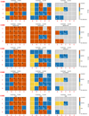 |
Fig. A.3 Same as Fig. A.2, but only considering the pixels that are part of the disk image. |
| In the text | |
|
Fig. B.1 Disk estimations obtained with PCA, I-PCA (GreeDS), and mustard for cube #4 and disk E. Details on the empty data sets can be found in Table 2 and Sect. 4.1. The three pairs of rows correspond to different injected contrast levels: 10−3 (top), 10−4 (middle), and 10−5 (bottom). The top row of each pair shows the estimations, while the bottom row shows the residuals. Each column displays the following: GT (left), PCA (middle-left), I-PCA (middle-right), and mustard (right). The best method, as determined by each metric, is indicated in the bottom-left corner of each pair of rows. More details are provided in the text of Appendix B. |
| In the text | |
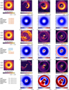 |
Fig. B.2 Same as Fig B.1, but for the case of cube #4 and disk D. |
| In the text | |
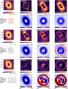 |
Fig. B.3 Same as Fig B.1, but for the case of cube #4 and disk C. Article number. |
| In the text | |
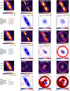 |
Fig. B.4 Same as Fig B.1, but for the case of cube #4 and disk B. |
| In the text | |
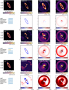 |
Fig. B.5 Same as Fig B.1, but for the case of cube #4 and disk A. |
| In the text | |
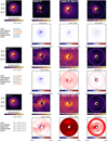 |
Fig. B.6 Same as Fig B.1, but for the case of cube #3 and disk E. |
| In the text | |
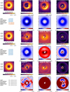 |
Fig. B.7 Same as Fig B.1, but for the case of cube #3 and disk D. |
| In the text | |
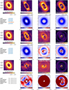 |
Fig. B.8 Same as Fig B.1, but for the case of cube #3 and disk C. |
| In the text | |
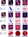 |
Fig. B.9 Same as Fig B.1, but for the case of cube #3 and disk B. |
| In the text | |
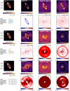 |
Fig. B.10 Same as Fig B.1, but for the case of cube #3 and disk A. |
| In the text | |
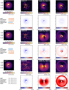 |
Fig. B.11 Same as Fig B.1, but for the case of cube #2 and disk E. |
| In the text | |
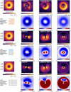 |
Fig. B.12 Same as Fig B.1, but for the case of cube #2 and disk D. |
| In the text | |
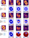 |
Fig. B.13 Same as Fig B.1, but for the case of cube #2 and disk C. |
| In the text | |
 |
Fig. B.14 Same as Fig B.1, but for the case of cube #2 and disk B. |
| In the text | |
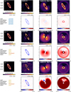 |
Fig. B.15 Same as Fig B.1, but for the case of cube #2 and disk A. |
| In the text | |
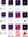 |
Fig. B.16 Same as Fig B.1, but for the case of cube #1 and disk E. |
| In the text | |
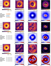 |
Fig. B.17 Same as Fig B.1, but for the case of cube #1 and disk D. |
| In the text | |
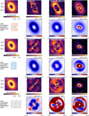 |
Fig. B.18 Same as Fig B.1, but for the case of cube #1 and disk C. |
| In the text | |
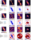 |
Fig. B.19 Same as Fig B.1, but for the case of cube #1 and disk B. |
| In the text | |
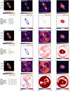 |
Fig. B.20 Same as Fig B.1, but for the case of cube #1 and disk A. |
| In the text | |
Current usage metrics show cumulative count of Article Views (full-text article views including HTML views, PDF and ePub downloads, according to the available data) and Abstracts Views on Vision4Press platform.
Data correspond to usage on the plateform after 2015. The current usage metrics is available 48-96 hours after online publication and is updated daily on week days.
Initial download of the metrics may take a while.